Q-Search Trees: An Information-Theoretic Approach Towards Hierarchical Abstractions for Agents with Computational Limitations

Abstract

In this paper, we develop a framework to obtain graph abstractions for decision-making by an agent where the abstractions emerge as a function of the agent’s limited computational resources. We discuss the connection of the proposed approach with information-theoretic signal compression, and formulate a novel optimization problem to obtain tree-based abstractions as a function of the agent’s computational resources. The structural properties of the new problem are discussed in detail, and two algorithmic approaches are proposed to obtain solutions to this optimization problem. We discuss the quality of, and prove relationships between, solutions obtained by the two proposed algorithms. The framework is demonstrated to generate a hierarchy of abstractions for a non-trivial environment.

1 Introduction

Information theory provides a principled framework for obtaining optimal compressed representations of a signal [1]. The ability to form such compressed representations, also known as abstractions, has widespread uses in many fields, ranging from signal processing and data transmission, to robotic motion planning in complex environments, and many others [2, 3, 4, 1, 5, 6, 7, 8, 9, 10, 11, 12, 13, 14, 15, 16, 17, 18]. Particularly for autonomous systems, simplified representations of the environment which the agent operates in are preferred, as they decrease the on-board memory requirements and reduce the computational time required to find feasible or optimal solutions for planning [9, 10, 11, 12, 2, 5, 6, 13, 8, 7, 19].

Within the realm of robotics and autonomous systems, a number of studies have leveraged the power of abstractions for both exploration and path-planning purposes. Examples of such prior works include [9, 10, 11, 12] in which wavelets were utilized in order to generate multi-resolution representations of two-dimensional environments. These compressed representations encode a simplified graph of the environment, speeding up the execution time of path-planning algorithms such as A^∗[5]. As the agent traverses the environment, the problem is sequentially re-solved in order to obtain a trade-off in the overall optimality of the resulting path, planning frequency, and obstacle avoidance. Similarly related work includes that of [5] and [6], where the authors employed a tree-based framework in order to execute path-planning tasks in two- and three-dimensional environments. In these studies, the planning problem involved the generation of a multi-resolution representation of the operating space of the agent in the form of a variable-depth probabilistic quadtree or octree, based on user-provided parameters and a given initial representation of the environment. Since that framework uses probabilistic quadtrees and octrees, the initial representation of the environment is in the form of an occupancy grid, allowing for the incorporation of sensor uncertainty when creating maps of the environment [20].

Other works have studied the generation of quadtrees in real time, such as [13], or the creation of multi-resolution trees from a given map and pruning rules [8]. Abstractions have also been proposed in the reinforcement learning (RL) community in order to alleviate the curse of dimensionality, allowing for the solution of larger problems [4, 21]. However, there is no unifying method for how these abstractions are generated, as existing methods rely heavily on user-provided rules.

The drawback of all these previous works is that they do not directly address the generation of the abstractions, and instead rely on them to be either provided a-priori or created in a manner that is known beforehand. Furthermore, existing works do not consider the computational limitations of the agent. That is, existing works do not consider in their formulation that agents with limited on-board resources may not employ the same representation, or depiction, of the environment as agents that are not resource limited. The idea that all agents do not have equal capabilities has been recently discussed in the literature pertaining to the field of bounded rationality [22, 23, 24]. In this point of view, the capabilities of an agent are represented by its information-processing abilities. Thus, a resource-limited agent is not able to process all data collected by observing its surroundings, leading to the need for simplification of the space in which it operates. Utilizing these abstract representations precludes the agent from necessarily finding globally optimal solutions, but induces policies that require the agent to process fewer details of the environment in order to act [22, 25, 23, 18].

A number of existing works have modeled single-stage and sequential bounded-rational decision making in stochastic domains by employing ideas from utility and information theory to construct constrained optimization problems [22, 18, 23, 24]. The solution to these problems is a set of self-consistent equations, which are numerically solved by alternating iterations analogous to the Blahut-Arimoto algorithm in rate-distortion theory [23, 22, 26, 18]. Interestingly, this framework allows for the emergence of bounded-rational policies for a range of agents with varying capabilities, recovering the rational solution in the limit [18, 23, 24, 22].

In this paper, we address the issue of abstraction generation for a given environment, and formulate a novel optimization problem that leverages concepts from information theory to obtain representations of an environment that are a function of the agent’s available resources. Specifically, we consider the case where the environment is represented as a multi-resolution quadtree, and begin by discussing connections between environment abstractions in the form of quadtrees and general signal compression, the latter of which has been extensively studied by information theorists. We then formulate an optimization problem over the space of trees that utilizes concepts from the information bottleneck method [26], and we subsequently propose two algorithms to solve the problem. Theoretical guarantees of our proposed algorithmic approaches are presented and discussed. The approach is applied to a non-trivial example, where we examine the results and discuss the interpretation of the theory as applied to bounded-rational agents.

The remainder of the paper is organized as follows. In Section 2 we introduce and review the fundamental concepts needed in this work as well as we review the connections between quadtrees and optimal signal compression. Then, in Section 3, we formulate our problem and show how principles from information theory can be incorporated into a new optimization problem over the space of trees. In Section 4, we propose two algorithms that can be used to solve the optimization problem and present the theoretical contributions of the paper. Section 5 presents results of the proposed methodology applied to an occupancy grid with and without prior information. We conclude with several remarks in Section 6.

2 Preliminaries

2.1 Quadtree Decompositions

We consider the emergence of abstractions in the form of multi-resolution quadtree representations. Quadtrees are a common tool utilized in the robotics community to reduce the complexity of environments in order to speed path-planning or ease internal storage requirements [5, 6, 2, 13, 16]. The theoretical contributions of the paper are applicable however for any tree structure, beyond just quadtrees. To this end, we assume that the environment $\mathcal{W}\subset\mathbb{R}^{2}$ (generalizable to $\mathbb{R}^{d}$) is given by a two-dimensional grid world where each grid element is a unit square (hypercube). We assume that there exists an integer $\ell>0$ such that $\mathcal{W}$ is contained within a square (hypercube) of side length $2^{\ell}$. A tree representation $\mathcal{T}=\left(\mathcal{N},\mathcal{E}\right)=\left(\mathcal{N}(\mathcal{T}),\mathcal{E}(\mathcal{T})\right)$ of $\mathcal{W}$ consists of a set of nodes $\mathcal{N}$ and edges $\mathcal{E}$ describing the interconnections between the nodes in the tree [6]. We denote the set of all possible quadtree representations of maximum depth $\ell$ of $\mathcal{W}$ by $\mathcal{T}^{\mathcal{Q}}$ and let $\mathcal{T}_{\mathcal{W}}\in\mathcal{T}^{\mathcal{Q}}$ denote the finest quadtree representation of $\mathcal{W}$; an example is shown in Figure 2. It should be noted that $\mathcal{T}_{\mathcal{W}}$ encodes a specific structure for $\mathcal{W}$, which we make precise in the following definition.

Definition 2.1

Let $t\in\mathcal{N}(\mathcal{T}_{\mathcal{W}})$ be any node at depth $k\in\left\{0,\ldots,\ell\right\}$. Then $t^{\prime}\in\mathcal{N}(\mathcal{T}_{\mathcal{W}})$ is a child of $t$ if the following hold:

1. Node $t^{\prime}$ is at depth $k+1$ in $\mathcal{T}_{\mathcal{W}}$.

2. Nodes $t$ and $t^{\prime}$ are incident to a common edge, i.e., $\left(t,t^{\prime}\right)\in\mathcal{E}\left(\mathcal{T}_{\mathcal{W}}\right)$.

Conversely, we say that $t$ is the parent of $t^{\prime}$ if $t^{\prime}$ is a child of $t$. Furthermore, we let

$$\mathcal{N}_{k}(\mathcal{T}_{q})=\left\{t\in\mathcal{N}(\mathcal{T}_{q}):t\text{~{}is at depth~{}}k~{}\text{in}~{}\mathcal{T}_{\mathcal{W}}\right\},$$

to be the set of all nodes of the tree $\mathcal{T}_{q}\in\mathcal{T}^{\mathcal{Q}}$ at depth $k$.

We will frequently seek to relate nodes in the tree $\mathcal{T}_{q}$ to those in the tree $\mathcal{T}_{\mathcal{W}}$, which leads us to the following definition.

Definition 2.2

Let $t\in\mathcal{N}(\mathcal{T}_{q})$ be any node in the tree $\mathcal{T}_{q}\in\mathcal{T}^{\mathcal{Q}}$. Then the following hold:

1. The node $t$ has children

   $$\mathcal{C}(t)=\left\{t^{\prime}\in\mathcal{N}(\mathcal{T}_{\mathcal{W}}):t^{\prime}\text{~{}is a child of~{}}t\right\}.$$

2. The node $t$ has parent

   $$\mathcal{P}(t)=\left\{\hat{t}\in\mathcal{N}(\mathcal{T}_{\mathcal{W}}):t\in\mathcal{C}(\hat{t})\right\}.$$

3. The node $t$ is the root of the tree $\mathcal{T}_{q}$, denoted by $\mathrm{Root}\left(\mathcal{T}_{q}\right)$, if $\mathcal{P}(t)=\emptyset$.

4. The node $t$ is a leaf of $\mathcal{T}_{q}$ if $\mathcal{C}(t)\cap\mathcal{N}(\mathcal{T}_{q})=\emptyset$. Furthermore, the set of leaf nodes of $\mathcal{T}_{q}$ is given by

   $$\mathcal{N}_{\text{leaf}}\left(\mathcal{T}_{q}\right)=\left\{t^{\prime}\in\mathcal{N}(\mathcal{T}_{q}):\mathcal{C}(t^{\prime})\cap\mathcal{N}(\mathcal{T}_{q})=\emptyset\right\}.$$

5. If $t\notin\mathcal{N}_{\text{leaf}}(\mathcal{T}_{q})$ then $t\in\mathcal{N}_{\text{int}}(\mathcal{T}_{q})=\mathcal{N}(\mathcal{T}_{q})\setminus\mathcal{N}_{\text{leaf}}(\mathcal{T}_{q})$, where $\mathcal{N}_{\text{int}}(\mathcal{T}_{q})$ is the set of interior nodes of $\mathcal{T}_{q}$.

Note that the space $\mathcal{T}^{\mathcal{Q}}$ encodes a specific structure on the abstractions of the environment, as shown in Figure 2. Specifically, each $\mathcal{T}_{q}\in\mathcal{T}^{\mathcal{Q}}$, $\mathcal{T}_{q}\neq\mathcal{T}_{\mathcal{W}}$, specifies a precise relation between the leaf nodes of $\mathcal{T}_{\mathcal{W}}$ and the leaf nodes of $\mathcal{T}_{q}$, an example of which is shown in Figures 2 and 2. That is, the tree $\mathcal{T}_{q}\in\mathcal{T}^{\mathcal{Q}}$ specifies an abstraction for which the leaf nodes of $\mathcal{T}_{\mathcal{W}}$ are mapped to leaf nodes of $\mathcal{T}_{q}$ in such a way that $\mathcal{T}_{q}$ is a pruned quadtree representation of $\mathcal{W}$. An alternative way to view this is to consider each $\mathcal{T}_{q}\in\mathcal{T}^{\mathcal{Q}}$ as a pruned version of $\mathcal{T}_{\mathcal{W}}$, where some nodes in the interior of $\mathcal{T}_{\mathcal{W}}$ are leaf nodes of $\mathcal{T}_{q}$. In this way, we can consider each $\mathcal{T}_{q}\in\mathcal{T}^{\mathcal{Q}}$ as encoding an abstraction, or compression, of $\mathcal{W}$ with a constraint that $\mathcal{T}_{q}$ be a valid quadtree depiction of $\mathcal{W}$.

Figure 1: Representation of the tree $\mathcal{T}_{\mathcal{W}}$ and corresponding grid for a $4\times 4$ environment.

Figure 2: Representation of some $\mathcal{T}_{q}\in\mathcal{T}^{\mathcal{Q}}$ and corresponding grid for a $4\times 4$ environment.

Per the above discussion, varying the abstraction granularity of $\mathcal{W}$ can be equivalently viewed as selecting various trees $\mathcal{T}_{q}$ in the space $\mathcal{T}^{\mathcal{Q}}$. Our problem is then one of selecting a tree $\mathcal{T}_{q}\in\mathcal{T}^{\mathcal{Q}}$ as a function of the agent’s computational capabilities.

The observation that each $\mathcal{T}_{q}\in\mathcal{T}^{\mathcal{Q}}$ encodes a compression of $\mathcal{W}$ connects our approach to information-theoretic frameworks that consider optimal encoder design. The optimization problem to obtain optimal encoders has been extensively studied by information theorists in the more general setting of signal compression, where no specific structure on the abstraction is enforced (i.e., the resulting encoding need not correspond to any tree representation). As such, the added constraint that our abstraction be a valid quadtree representation of $\mathcal{W}$ creates additional challenges, since direct application of information-theoretic methods is not possible. Thus, to elucidate the technical aspects of our approach, we first present a brief review of the necessary information-theoretical concepts which we will utilize in the formulation of our problem.

2.2 Information-Theoretical Signal Compression

The task of obtaining optimal compressed representations of signals is addressed within the realm of information theory [26, 27, 28, 29, 1, 30]. Let $\left(\Omega,\mathcal{F},\mathbb{P}\right)$ to be a probability space with finite sample space $\Omega$, $\sigma$-algebra $\mathcal{F}$ and probability measure $\mathbb{P}:\mathcal{F}\to\left[0,1\right]$, and denote the set of real and positive real numbers as $\mathbb{R}$ and $\mathbb{R}_{++}$, respectively. Let $X:\Omega\to\mathbb{R}$ denote the random variable corresponding to the original, uncompressed, signal, where $X$ takes values in the set $\Omega_{X}=\left\{x\in\mathbb{R}:X(\omega)=x,~{}\omega\in\Omega\right\}$ and, for any $x\in\mathbb{R}$, $p(x)=\mathbb{P}(\left\{\omega\in\Omega:X(\omega)=x\right\})$. Furthermore, let the random variable $T:\Omega\to\mathbb{R}$ denote the compressed representation of $X$, where $T$ takes values in the set $\Omega_{T}=\left\{t\in\mathbb{R}:T(\omega)=t,~{}\omega\in\Omega\right\}$. The level of compression between random variables $X$ and $T$ is measured by the mutual information [26, 1], given by

$$I(T;X)\triangleq\sum_{t,x}p(t,x)\log\frac{p(t,x)}{p(t)p(x)}.$$ (1)

The goal is then to find a stochastic mapping (encoder), denoted $p(t|x)$, which maps outcomes in the uncompressed space $x\in\Omega_{X}$, to outcomes in the compressed representation $t\in\Omega_{T}$ so as to minimize $I(T;X)$ (maximize compression) [26]. However, in order to obtain non-trivial solutions, a metric quantifying the quality of the resulting compression must be introduced, since maximal compression $\left(I(T;X)=0\right)$ is always achievable. The information bottleneck (IB) method [26] defines the quality of the compression utilizing mutual information.

More specifically, the IB method introduces an additional random variable, $Y:\Omega\to\mathbb{R}$, taking values in the set $\Omega_{Y}=\left\{y\in\mathbb{R}:Y(\omega)=y,~{}\omega\in\Omega\right\}$. The variable $Y$ represents information we are interested in preserving when forming the compressed representation $T$ [26, 27]. The method imposes the Markov chain condition $T\leftrightarrow X\leftrightarrow Y$ which arises as a consequence of the problem formulation. To see this, note that $p(y|t,x)=p(y|x)$ since it is not possible for $t$ to convey any additional information regarding $y$ than what is already in $x$, and thus $T\rightarrow X\rightarrow Y$. Furthermore, if $p(y|t,x)=p(y|x)$ then $p(t|y,x)=p(t|x)$ which gives $Y\rightarrow X\rightarrow T$. Therefore, $T\rightarrow X\rightarrow Y$ implies $Y\rightarrow X\rightarrow T$, which is written as $T\leftrightarrow X\leftrightarrow Y$ [1, 26].

The IB problem is then formulated as

$$\min_{p(t|x)}~{}I(T;X),$$ (2)

subject to

$$I(T;Y)\geq\hat{D},$$ (3)

where the minimization is done over all normalized distributions $p(t|x)$ assuming that the joint distribution $p(x,y)$ is provided and $\hat{D}\geq 0$ [26]. Through the introduction of a Lagrange multiplier, $\beta\geq 0$, we have that (2) subject to (3) has Lagrangian

$$\mathcal{K}_{Y}(p(t|x);\beta)\triangleq I(T;X)-\beta I(T;Y).$$ (4)

Furthermore, for given $\beta\geq 0$, the optimization problem

$$\min_{p(t|x)}~{}\mathcal{K}_{Y}(p(t|x);\beta),$$ (5)

can be solved analytically, giving rise to a set of self-consistent equations [26].

The self-consistent equations obtained as a solution to (5) can be solved numerically by an algorithm that likens that of the Blahut-Arimoto algorithm from rate-distortion theory, albeit with no guarantee of convergence to a globally optimal solution [26]. The parameter $\beta$ serves the role of adjusting the amount of relevant information regarding $Y$ that is retained in the abstract representation $T$. As a result, when $\beta\to\infty$ the optimization process is concerned with the maximal preservation of information, while $\beta\to 0$ promotes maximal compression, with no regard to the information carried regarding $Y$. Intermediate values of $\beta$ lead to a spectrum of solutions between these two extremes [26]. The mapping $p^{*}(t|x)$ obtained as a solution to the IB problem is generally stochastic, resulting in a deterministic mapping only when $\beta\to\infty$ [29, 26].

2.3 Agglomerative Information Bottleneck

The agglomerative IB (AIB) method is another framework to form compressed representations of $X$, which is useful when deterministic clusters that retain predictive information regarding the relevant variable $Y$ are desired. The method uses the IB approach to solve for deterministic, or hard, encoders (i.e., $p(t|x)\in\left\{0,1\right\}$ for all $t$, $x$). Concepts from AIB will prove useful in our formulation, since each tree $\mathcal{T}_{q}\in\mathcal{T}^{\mathcal{Q}}$ encodes a hard (deterministic) abstraction of $\mathcal{W}$, where each leaf node of $\mathcal{T}_{\mathcal{W}}$ is aggregated to a specific leaf node of $\mathcal{T}_{q}$. That is, by viewing the uncompressed space ($\Omega_{X}$) as the nodes in $\mathcal{N}_{\text{leaf}}(\mathcal{T}_{\mathcal{W}})$ and the abstracted (compressed) space ($\Omega_{T}$) as the nodes in $\mathcal{N}_{\text{leaf}}(\mathcal{T}_{q})$, the abstraction operation can be specified in terms of an encoder $p(t|x)$ where $p(t|x)\in\left\{0,1\right\}$ for all $t$ and $x$, where $p(t|x)=1$ if $x\in\mathcal{N}_{\text{leaf}}(\mathcal{T}_{\mathcal{W}})$ is aggregated to $t\in\mathcal{N}_{\text{leaf}}(\mathcal{T}_{q})$, and zero otherwise (see Figures 2 and 2). To better understand these connections, we briefly review the AIB before presenting the formulation of our problem.

The solution provided by AIB is an encoder $p(t|x)$ for which $p(t|x)\in\left\{0,1\right\}$ for all $t$, $x$ and $\beta>0$. AIB considers the optimization problem

$$\max_{p(t|x)}~{}\mathcal{L}_{Y}(p(t|x);\beta),$$ (6)

where the Lagrangian is defined as

$$\mathcal{L}_{Y}(p(t|x);\beta)\triangleq I(T;Y)-\frac{1}{\beta}I(T;X),$$ (7)

and the maximization is performed over deterministic distributions $p(t|x)$ for given $\beta>0$ and $p(x,y)$ [27, 28].

AIB works from bottom-up, starting with $T=X$ and with each consecutive iteration reduces the cardinality of $T$ until $\left|\Omega_{T}\right|=1$[27]. Specifically, let $T_{m}$ represent the abstracted space with $m$ elements $\left(\left|\Omega_{T_{m}}\right|=m\right)$ and let $T_{i}$ represent the compressed space with $\left|\Omega_{T_{i}}\right|=i<m$ elements, where $i=m-1$ and the number of merged elements is $n=2$. We then merge elements $\left\{t^{\prime}_{1},\ldots,t^{\prime}_{n}\right\}\subseteq\Omega_{T_{m}}$ to a single element $t\in\Omega_{T_{i}}$ to obtain $T_{i}$. The set $\left\{t^{\prime}_{1},\ldots,t^{\prime}_{n}\right\}\subseteq\Omega_{T_{m}}$ selected to merge is determined by considering the difference in the IB Lagrangian induced by the merge operation, as follows. Let $p^{-}:\Omega_{T_{m}}\times\Omega_{X}\to\left\{0,1\right\}$ be the mapping before the merge and $p^{+}:\Omega_{T_{i}}\times\Omega_{X}\to\left\{0,1\right\}$ be the resulting mapping after elements $\left\{t^{\prime}_{1},\ldots,t^{\prime}_{n}\right\}\subseteq\Omega_{T_{m}}$ are grouped to $t\in\Omega_{T_{i}}$. Note that, as AIB considers a sequence of merges, the mapping $p^{-}(t|x)$ represents an abstraction of higher cardinality as compared to $p^{+}(t|x)$. The merger cost is then given by $\Delta\mathcal{L}_{Y}:2^{\Omega_{T_{m}}}\times\mathbb{R}_{++}\to\mathbb{R}$, defined as [28]

$$\Delta\mathcal{L}_{Y}(\left\{t^{\prime}_{1},\ldots,t^{\prime}_{n}\right\};\beta)\triangleq\mathcal{L}_{Y}(p^{-}(t|x);\beta)-\mathcal{L}_{Y}(p^{+}(t|x);\beta).$$ (8)

The above relation can be decomposed into a change in mutual information by utilizing (7) as

$$\Delta\mathcal{L}_{Y}(\left\{t^{\prime}_{1},\ldots,t^{\prime}_{n}\right\};\beta)=\left[I(T_{m};Y)-I(T_{i};Y)\right]-\frac{1}{\beta}\left[I(T_{m};X)-I(T_{i};X)\right],$$ (9)

which can be further simplified by noting that

$$I(T;X)=H(T)-H(T|X)=H(T),$$ (10)

and where, since $p(t|x)\in\left\{0,1\right\}$, there is no uncertainty in $T$ once we are provided $x\in\Omega_{X}$ leading to $H(T|X)=0$. Thus, equation (9) becomes

$$\Delta\mathcal{L}_{Y}(\left\{t^{\prime}_{1},\ldots,t^{\prime}_{n}\right\};\beta)=\left[I(T_{m};Y)-I(T_{i};Y)\right]-\frac{1}{\beta}\left[H(T_{m})-H(T_{i})\right].$$ (11)

It was shown in [27, 28] that (11) can be written as

$$\Delta\mathcal{L}_{Y}(\left\{t^{\prime}_{1},\ldots,t^{\prime}_{n}\right\};\beta)=p(t)\left[\mathrm{JS}_{\Pi}(p(y|t^{\prime}_{1}),\ldots,p(y|t^{\prime}_{n}))-\frac{1}{\beta}H(\Pi)\right],$$ (12)

where $\Pi\in\mathbb{R}^{n}$ is given as

$$\Pi=\left[\Pi_{1},\ldots,\Pi_{n}\right]^{\mathsf{T}}\triangleq\left[\frac{p(t^{\prime}_{1})}{p(t)},\ldots,\frac{p(t^{\prime}_{n})}{p(t)}\right]^{\mathsf{T}},$$ (13)

and $\mathrm{JS}_{\Pi}(p_{1},\ldots,p_{n})$ is the Jensen-Shannon (JS) divergence between the distributions $p_{1},\ldots,p_{n}$, with weights $\Pi$ defined as [31]

$$\mathrm{JS}_{\Pi}(p_{1},\ldots,p_{n})\triangleq\sum_{s=1}^{n}\Pi_{s}\mathrm{D}_{\mathrm{KL}}(p_{s},\bar{p}),$$ (14)

where, for each outcome $y\in\Omega_{Y}$,

$$\bar{p}(y)=\sum_{s=1}^{n}\Pi_{s}p_{s}(y),$$ (15)

with $\mathrm{D}_{\mathrm{KL}}(\mu,\nu)$ denoting the Kullback-Leibler (KL) divergence between probability distributions $\mu$ and $\nu$ given by

$$\mathrm{D}_{\mathrm{KL}}(\mu,\nu)\triangleq\sum_{y}\mu(y)\log\frac{\mu(y)}{\nu(y)}.$$ (16)

Furthermore, we have that

$$p(t) =\sum_{s=1}^{n}p(t^{\prime}_{s}),$$ (17)

$$p(y|t) =\sum_{s=1}^{n}\Pi_{s}p(y|t^{\prime}_{s}),$$ (18)

which can be found by realizing that $p(t|x)\in\left\{0,1\right\}$ for all $x\in\Omega_{X}$ and $t\in\Omega_{T}$ and $T\leftrightarrow X\leftrightarrow Y$[27, 28]. Note that the merger cost (8) can be written in terms of the distributions $p(y|t^{\prime}_{1}),\ldots,p(y|t^{\prime}_{n})$ and the weight vector $\Pi$. This reduces the overall complexity of computing $\Delta\mathcal{L}_{Y}(\left\{t^{\prime}_{1},\ldots,t^{\prime}_{n}\right\};\beta)$ as opposed to utilizing equation (9), which contains sums over the sample spaces of $Y$, $T$ and $X$ [27, 28].

3 Problem Formulation

The IB methods presented in the previous section do not impose any constraints on the resulting mapping $p(t|x)$. That is, by solving the IB problem, one obtains a mapping $p^{*}(t|x)$ that is generally stochastic, and thus it is not guaranteed that it encodes a (quad)tree representation for any value of $\beta>0$. The difficulty lies in the specific structure imposed on the abstraction by the space $\mathcal{T}^{\mathcal{Q}}$, as even AIB or deterministic IB cannot guarantee that the resulting $p^{*}(t|x)$ encode a tree belonging to $\mathcal{T}^{\mathcal{Q}}$, although they do provide deterministic encoders [29, 27, 28]. Recall that, since each $\mathcal{T}_{q}\in\mathcal{T}^{\mathcal{Q}}$ represents an abstraction of $\mathcal{T}_{\mathcal{W}}$, $\mathcal{T}_{q}$ can be equivalently represented as $p^{q}(t|x)$, where $p^{q}(t|x)=1$ if $x\in\mathcal{N}_{\text{leaf}}(\mathcal{T}_{\mathcal{W}})$ is abstracted to $t\in\mathcal{N}_{\text{leaf}}(\mathcal{T}_{q})$ and zero otherwise. We can then define the IB Lagrangian in the space of quadtrees as the mapping $L_{Y}:\mathcal{T}^{\mathcal{Q}}\times\mathbb{R}_{++}\to\mathbb{R}$ given by

$$L_{Y}(\mathcal{T}_{q};\beta)\triangleq\mathcal{L}_{Y}(p^{q}(t|x);\beta),$$ (19)

where $\mathcal{L}_{Y}(p(t|x);\beta)$ is defined in (7). Then, for a given $\beta>0$, we can search the space of trees for the one that maximizes (19). This optimization problem is formally given by

$$\mathcal{T}_{q^{*}}=\hskip 4.26773pt\stackrel{{\scriptstyle[}}{{\mathcal{}}}T_{q}\in\mathcal{T}^{\mathcal{Q}}]{}{\operatorname{argmax}}L_{Y}(\mathcal{T}_{q};\beta).$$ (20)

The resulting world representation is encoded by the mapping $p^{q^{*}}(t|x)$. That is, the leafs of $\mathcal{T}_{q^{*}}$ determine the optimal multi-resolution representation of $\mathcal{W}$ for the given $\beta$.

By posing the optimization problem as in (20), we have implicitly incorporated the constraints on the mapping $p(t|x)$ in order for the resulting representation to be a quadtree depiction of the world. While the optimization problem given by (20) allows one to form an analogous problem to that in (6) over the space of trees, the drawback of this method is the need to exhaustively enumerate all feasible quadtrees which can represent the space. In other words, (20) requires that $p^{q}(t|x)$ be provided for each $\mathcal{T}_{q}\in\mathcal{T}^{\mathcal{Q}}$. Because of this, the problem becomes intractable for large grid sizes and thus requires reformulation to handle larger world maps.

Figure 3: Sequence of trees from $\mathcal{T}_{q^{0}}=\mathrm{Root}(\mathcal{T}_{\mathcal{W}})\in\mathcal{T}^{\mathcal{Q}}$ to $\mathcal{T}_{q^{m}}\in\mathcal{T}^{\mathcal{Q}}$ ($m=3$) by performing only a sequence of nodal expansions. Note that $\mathcal{T}_{q^{0}}=\mathrm{Root}\left(\mathcal{T}_{\mathcal{W}}\right)$ is the root node of $\mathcal{T}_{\mathcal{W}}$.

Interestingly, we note that it is possible to arrive at a quadtree $\mathcal{T}_{q^{m}}\in\mathcal{T}^{\mathcal{Q}}$ starting from $\mathcal{T}_{q^{0}}\in\mathcal{T}^{\mathcal{Q}}$ and performing a sequence of expansions, as illustrated in Figure 3. The resulting sequence of expansions can be viewed as defining a path between $\mathcal{T}_{q^{0}}$ and $\mathcal{T}_{q^{m}}$, in which each vertex of the path corresponds to a distinct intermediate tree in the sequence. It should be noted that by considering this sequence of expansions it is not always possible to reach any tree $\mathcal{T}_{q^{m}}$ starting from any tree $\mathcal{T}_{q^{0}}$. In order to address this, we first require the following definitions.

Definition 3.1 ([32])

A tree $\mathcal{G}=(\mathcal{N}(\mathcal{G}),\mathcal{E}(\mathcal{G}))$ is a subtree of the tree $\mathcal{J}=\left(\mathcal{N}(\mathcal{J}),\mathcal{E}(\mathcal{J})\right)$, denoted $\mathcal{G}\subseteq\mathcal{J}$, if $\mathcal{N}(\mathcal{G})\subseteq\mathcal{N}(\mathcal{J})$ and $\mathcal{E}(\mathcal{G})\subseteq\mathcal{E}(\mathcal{J})$.

Definition 3.2

The trees $\mathcal{T}_{q^{\prime}}\in\mathcal{T}^{\mathcal{Q}}$ and $\mathcal{T}_{q}\in\mathcal{T}^{\mathcal{Q}}$ are neighbors if $\mathcal{N}(\mathcal{T}_{q^{\prime}})\setminus\mathcal{N}(\mathcal{T}_{q})=\left\{t^{\prime}_{1},\ldots,t^{\prime}_{n}\right\}\subseteq\mathcal{N}_{\text{leaf}}(\mathcal{T}_{q^{\prime}})$ such that $t=\mathcal{P}(t^{\prime}_{1})=\cdots=\mathcal{P}(t^{\prime}_{n})\in\mathcal{N}_{\text{leaf}}(\mathcal{T}_{q})$ or $\mathcal{N}(\mathcal{T}_{q})=\mathcal{N}(\mathcal{T}_{q^{\prime}})\setminus\left\{t^{\prime}_{1},\ldots,t^{\prime}_{n}\right\}$ where $\left\{t^{\prime}_{1},\ldots,t^{\prime}_{n}\right\}\subseteq\mathcal{N}_{\text{leaf}}(\mathcal{T}_{q^{\prime}})$ have common parent $t=\mathcal{P}(t^{\prime}_{1})=\cdots=\mathcal{P}(t^{\prime}_{n})\in\mathcal{N}_{\text{leaf}}(\mathcal{T}_{q})$.

With these definitions, we see that if $\mathcal{T}_{q^{\prime}}\in\mathcal{T}^{\mathcal{Q}}$ is a neighbor of $\mathcal{T}_{q}\in\mathcal{T}^{\mathcal{Q}}$, then we can obtain $\mathcal{T}_{q^{\prime}}$ by adding the nodes $\left\{t^{\prime}_{1},\ldots,t^{\prime}_{n}\right\}$ to $\mathcal{T}_{q}$, where the set $\left\{t^{\prime}_{1},\ldots,t^{\prime}_{n}\right\}$ consists of the children of a leaf node of $\mathcal{T}_{q}$. We call this process of adding $\left\{t^{\prime}_{1},\ldots,t^{\prime}_{n}\right\}$ to $\mathcal{N}(\mathcal{T}_{q})$ a nodal expansion. We observe that by only performing a sequence of nodal expansions, a path exists between the trees $\mathcal{T}_{q^{0}}\in\mathcal{T}^{\mathcal{Q}}$ and $\mathcal{T}_{q^{m}}\in\mathcal{T}^{\mathcal{Q}}$ if $\mathcal{T}_{q^{0}}$ is a subtree of $\mathcal{T}_{q^{m}}$ $\left(\mathcal{T}_{q^{0}}\subseteq\mathcal{T}_{q^{m}}\right)$. An illustration of nodal expansion is provided in Figure 3, where we also note that each tree $\mathcal{T}_{q^{i+1}}$ in the sequence is a neighbor to tree $\mathcal{T}_{q^{i}}$ with $i\in\left\{0,1,2\right\}$.

Furthermore, we may view the set of all possible quadtrees as a connected graph, where neighbors are defined according to Definition 3.2. An illustration of neighboring trees is provided in Figure 4. Thus, if it is possible to obtain a sequential characterization of (19), we can formulate an optimization problem requiring the generation of candidate solutions only along the path leading from $\mathcal{T}_{q^{0}}$ to $\mathcal{T}_{q^{m}}$. To this end, if we take $\mathcal{T}_{q^{0}}\subseteq\mathcal{T}_{q^{m}}$, where $\mathcal{T}_{q^{0}},\mathcal{T}_{q^{m}}\in\mathcal{T}^{\mathcal{Q}}$, and assume that $\mathcal{T}_{q^{m}}$ is obtained by $m$ expansions of $\mathcal{T}_{q^{0}}$, then

$$L_{Y}(\mathcal{T}_{q^{m}};\beta)=L_{Y}(\mathcal{T}_{q^{0}};\beta)+\sum_{i=0}^{m-1}\Delta L_{Y}(\mathcal{T}_{q^{i}},\mathcal{T}_{q^{i+1}};\beta),$$ (21)

where $\Delta L_{Y}(\cdot,\cdot;\beta)$ is defined as

$$\Delta L_{Y}(\mathcal{T}_{q^{i}},\mathcal{T}_{q^{i+1}};\beta)\triangleq L_{Y}(\mathcal{T}_{q^{i+1}};\beta)-L_{Y}(\mathcal{T}_{q^{i}};\beta),$$ (22)

and $\mathcal{T}_{q^{i+1}}\in\mathcal{T}^{\mathcal{Q}}$ is a neighbor of $\mathcal{T}_{q^{i}}\in\mathcal{T}^{\mathcal{Q}}$ with higher leaf node cardinality for $i\in\left\{0,\ldots,m-1\right\}$. Consequently, (21) gives a sequential representation of (19). Furthermore, the nodal expansion operation to move from tree $\mathcal{T}_{q}\in\mathcal{T}^{\mathcal{Q}}$ to the neighbor $\mathcal{T}_{q^{\prime}}\in\mathcal{T}^{\mathcal{Q}}$ has an analogous interpretation to the AIB method discussed in Section 2. Consequently,

$$\Delta L_{Y}(\mathcal{T}_{q^{i}},\mathcal{T}_{q^{i+1}};\beta)=\Delta\mathcal{L}_{Y}(\left\{t^{\prime}_{1},\ldots,t^{\prime}_{n}\right\};\beta),$$ (23)

and thus

$$\Delta L_{Y}(\mathcal{T}_{q^{i}},\mathcal{T}_{q^{i+1}};\beta)=p(t)\left[\mathrm{JS}_{\Pi}(p(y|t^{\prime}_{1}),\ldots,p(y|t^{\prime}_{n}))-\frac{1}{\beta}H(\Pi)\right].$$ (24)

Importantly, note that the structure of $\Delta L_{Y}(\mathcal{T}_{q^{i}},\mathcal{T}_{q^{i+1}};\beta)$ in (24) only depends on which leafs nodes of $\mathcal{T}_{q^{i}}$ are expanded, as depicted in Figure 5. This implies that $\Delta L_{Y}(\mathcal{T}_{q^{i}},\mathcal{T}_{q^{i+1}};\beta)$ is only a function of the nodes that are to be expanded, and not of the overall configuration of the tree, which greatly simplifies the calculation of $\Delta L_{Y}(\mathcal{T}_{q^{i}},\mathcal{T}_{q^{i+1}};\beta)$.

Figure 4: Tree neighbors of $\mathcal{T}_{q^{1}}=\left\{\mathcal{T}_{q^{2}},\mathcal{T}_{q^{3}},\mathcal{T}_{q^{4}},\mathcal{T}_{q^{5}}\right\}$ that are of higher leaf-node cardinality.

It follows that the optimization problem can be reformulated as

$$\max_{m}\max_{\left\{\mathcal{T}_{q^{1}},\ldots,\mathcal{T}_{q^{m}}\right\}}~{}L_{Y}(\mathcal{T}_{q^{0}};\beta)+\sum_{i=0}^{m-1}\Delta L_{Y}(\mathcal{T}_{q^{i}},\mathcal{T}_{q^{i+1}};\beta).$$ (25)

In this formulation, the constraint encoding that the resulting representation is a quadtree is handled implicitly by $\mathcal{T}_{q^{i}}\in\mathcal{T}^{\mathcal{Q}}$. The additional maximization over $m$ in (25) appears since the horizon of the problem is not known a-priori and is, instead, a free parameter in the optimization problem.

Next, we propose two algorithms that can be used to solve the problem in (25). Note that, by taking $\mathcal{T}_{q^{0}}=\mathrm{Root}(\mathcal{T}_{\mathcal{W}})\in\mathcal{T}^{\mathcal{Q}}$, we can guarantee that a path exists between $\mathcal{T}_{q^{0}}$ and any other $\mathcal{T}_{q}\in\mathcal{T}^{\mathcal{Q}}$, since, in this case, $\mathcal{T}_{q^{0}}\subseteq\mathcal{T}_{q}$ for all $\mathcal{T}_{q}\in\mathcal{T}^{\mathcal{Q}}$, as shown in Figure 3.

4 Algorithmic Solutions

In this section, we discuss two novel algorithmic approaches to solve the optimization problem (25). Specifically, we present two approaches: a Greedy search method, and an algorithm we call Q-tree search. Proofs of all lemmas, propositions and theorems in this section are provided in the appendix.

4.1 A Greedy Approach

Data: $p(x,y)$, $\beta>0$

1

Result: $\mathcal{T}_{q^{*}}$

2

3Initialize: $\mathcal{T}_{q^{0}}$, $i\leftarrow 0$, $\textit{Stop\_Flag}\leftarrow\texttt{False}$.

4while not Stop_Flag do

5      

6      for $\mathcal{T}_{q}$ neighbor of $\mathcal{T}_{q^{i}}$ do

7            

8            neighbor_vector $\leftarrow\Delta L_{Y}(\mathcal{T}_{q^{i}},\mathcal{T}_{q};\beta)$

9      

10      if $\max$ neighbor_vector $>0$ then

11            

12            $b\leftarrow\operatorname{argmax}$ neighbor_vector

13             $\mathcal{T}_{q^{i+1}}\leftarrow$ neighbor $\mathcal{T}_{q^{b}}$ of $\mathcal{T}_{q^{i}}$

14             $i\leftarrow i+1$

15      else

16             Stop_Flag $\leftarrow\texttt{True}$

17             $\mathcal{T}_{q^{*}}\leftarrow\mathcal{T}_{q^{i}}$

18      

Algorithm 1 The Greedy Algorithm.

A Greedy approach to solve (25) involves maximizing $\Delta L_{Y}(\mathcal{T}_{q^{i}},\mathcal{T}_{q^{i+1}};\beta)$ myopically at each step. That is, provided that $\mathcal{T}_{q^{i+1}}\in\mathcal{T}^{\mathcal{Q}}$ is a neighbor of $\mathcal{T}_{q^{i}}\in\mathcal{T}^{\mathcal{Q}}$, we consider the next tree $\mathcal{T}_{q^{i+1}}$ that maximizes the value of $\Delta L_{Y}(\mathcal{T}_{q^{i}},\mathcal{T}_{q^{i+1}};\beta)$, and we sequentially keep selecting trees ($\mathcal{T}_{q^{i+1}}\to\mathcal{T}_{q^{i+2}}\to\ldots$) until no further improvement is possible. In other words, the Greedy algorithm continues along the current path in the space of trees until it finds a tree $\mathcal{T}_{q^{i}}\in\mathcal{T}^{\mathcal{Q}}$ that has no neighbor $\mathcal{T}_{q^{i+1}}\in\mathcal{T}^{\mathcal{Q}}$ of $\mathcal{T}_{q^{i}}$ such that $\Delta L_{Y}(\mathcal{T}_{q^{i}},\mathcal{T}_{q^{i+1}};\beta)>0$. The process is detailed in Algorithm 1.

The Greedy algorithm is simple to implement and requires little pre-processing. However, one can construct examples for a given $\beta>0$ and $\mathcal{T}_{q^{i}}\in\mathcal{T}^{\mathcal{Q}}$ for which $\Delta L_{Y}(\mathcal{T}_{q^{i}},\mathcal{T}_{q^{i+1}};\beta)<0$ for all $\mathcal{T}_{q^{i+1}}\in\mathcal{T}^{\mathcal{Q}}$ that are neighbors of $\mathcal{T}_{q^{i}}$, and where there exists at least one neighbor $\mathcal{T}_{q^{i+2}}\in\mathcal{T}^{\mathcal{Q}}$ of $\mathcal{T}_{q^{i+1}}$ such that $\Delta L_{Y}(\mathcal{T}_{q^{i+1}},\mathcal{T}_{q^{i+2}};\beta)>0$ and $\Delta L_{Y}(\mathcal{T}_{q^{i}},\mathcal{T}_{q^{i+1}};\beta)+\Delta L_{Y}(\mathcal{T}_{q^{i+1}},\mathcal{T}_{q^{i+2}};\beta)>0$. This implies that the Greedy algorithm is not able to further improve the value of (25) at the current tree $\mathcal{T}_{q^{i}}$. In such a scenario, the algorithm will terminate at the condition $\Delta L_{Y}(\mathcal{T}_{q^{i}},\mathcal{T}_{q^{i+1}};\beta)<0$, without gaining access to $\Delta L_{Y}(\mathcal{T}_{q^{i+1}},\mathcal{T}_{q^{i+2}};\beta)>0$. Since in this scenario $\Delta L_{Y}(\mathcal{T}_{q^{i}},\mathcal{T}_{q^{i+1}};\beta)+\Delta L_{Y}(\mathcal{T}_{q^{i+1}},\mathcal{T}_{q^{i+2}};\beta)>0$, further improvement of (25) is possible, but not achievable by the Greedy approach. Therefore, while the Greedy algorithm is simple to implement, it does not, in general, find globally optimal solutions. However, as $\beta\to\infty$, the Greedy algorithm does find a global solution as $\lim_{\beta\to\infty}\Delta L_{Y}(\mathcal{T}_{q^{i}},\mathcal{T}_{q^{i+1}};\beta)\geq 0$ for all $\mathcal{T}_{q}\in\mathcal{T}^{\mathcal{Q}}$, as seen by the limit of (24) and non-negativity of the JS-divergence.

Figure 5: Representation of the invariance of $\Delta L_{Y}(\mathcal{T}_{q^{i}},\mathcal{T}_{q^{i+1}};\beta)$. In this case, $\Delta L_{Y}(\mathcal{T}_{q^{1}},\mathcal{T}_{q^{2}};\beta)=\Delta L_{Y}(\mathcal{T}_{q^{3}},\mathcal{T}_{q^{4}};\beta)$.

4.2 The Q-tree Search Algorithm

We now present another approach, detailed in Algorithm 2, designed to overcome some of the shortfalls encountered with the Greedy algorithm. The main drawback by utilizing the Greedy approach in solving the optimization problem (25) is the short-sightedness of the algorithm and its inability to realize that poor expansions at the current step may lead to much higher-valued options in the future. This is analogous to problems in reinforcement learning and dynamic programming, where an action-value function $\left(Q\text{-function}\right)$ is introduced to incorporate the notion of cost-to-go for selecting among feasible actions in a given state [3, 33]. The idea behind introducing such a function is to incorporate future costs, thus allowing agents to take actions that are not the most optimal with respect to the current one-step cost, but have lower total cost due to events that are possible in the future.

To this end, we define the function

$$Q_{Y}(\mathcal{T}_{q^{i}},\mathcal{T}_{q^{i+1}};\beta)\triangleq\max\left\{\Delta L_{Y}(\mathcal{T}_{q^{i}},\mathcal{T}_{q^{i+1}};\beta)+\sum_{\tau=1}^{n}Q_{Y}(\mathcal{T}_{q^{i+1}},\mathcal{T}_{q_{\tau}^{i+2}};\beta),~{}0\right\},$$ (26)

where $\mathcal{T}_{q^{i+1}}$ is a neighbor of $\mathcal{T}_{q^{i}}$ with higher leaf node cardinality and

$$Q_{Y}(\mathcal{T}_{q^{\prime}},\mathcal{T}_{\mathcal{W}};\beta)\triangleq\max\left\{\Delta L_{Y}(\mathcal{T}_{q^{\prime}},\mathcal{T}_{\mathcal{W}};\beta),~{}0\right\},$$ (27)

for all $\mathcal{T}_{q^{\prime}}\in\mathcal{T}^{\mathcal{Q}}$ for which $\mathcal{T}_{\mathcal{W}}\in\mathcal{T}^{\mathcal{Q}}$ is a neighbor. Hence, there exists a $t\in\mathcal{N}_{\text{leaf}}(\mathcal{T}_{q^{i}})$ for which $\mathcal{C}(t)=\left\{t^{\prime}_{1},\ldots,t^{\prime}_{n}\right\}=\mathcal{N}(\mathcal{T}_{q^{i+1}})\setminus\mathcal{N}(\mathcal{T}_{q^{i}})$. The quadtrees $\mathcal{T}_{q_{\tau}^{i+2}},~{}\tau\in\left\{1,\ldots,n\right\}$ are neighbors of $\mathcal{T}_{q^{i+1}}$ which are obtained by expanding the leaf nodes $t^{\prime}_{\tau}\in\mathcal{C}(t)$ for $\tau=1,\ldots,n$, as shown in Figure 6.

Figure 6: Illustration of $Q_{Y}(\mathcal{T}_{q^{i}},\mathcal{T}_{q^{i+1}};\beta)$ and its dependency on $Q_{Y}(\mathcal{T}_{q^{i+1}},\mathcal{T}_{q_{\tau}^{i+2}};\beta)$. Consider that the algorithm is at tree $\mathcal{T}_{q^{0}}$, represented by the single node $t_{0}$. Each of the nodes $\left\{t^{\prime}_{1},t^{\prime}_{2},t^{\prime}_{3},t^{\prime}_{4}\right\}=\left\{t_{1},t_{2},t_{3},t_{4}\right\}$, which are children of $t_{0}$, are expanded one by one to form the trees $\mathcal{T}_{q_{\tau}^{i+2}}$ for $\tau\in\left\{1,2,3,4\right\}$. Note that $n=4$ in (26) for the special case of quadtrees.

Data: $p(x,y)$, $\beta>0$

1

Result: $\mathcal{T}_{q^{*}}$

2

3Initialize: $\mathcal{T}_{q^{0}}$, $i\leftarrow 0$, $\textit{Stop\_Flag}\leftarrow\texttt{False}$, Populate $Q_{Y}(\mathcal{T}_{q^{i}},\mathcal{T}_{q^{i+1}};\beta)$.

4while not Stop_Flag do

5      

6      for $\mathcal{T}_{q}$ neighbor of $\mathcal{T}_{q^{i}}$ do

7            

8            neighbor_vector $\leftarrow Q_{Y}(\mathcal{T}_{q^{i}},\mathcal{T}_{q};\beta)$

9      

10      if $\max$ neighbor_vector $>0$ then

11            

12            $b\leftarrow\operatorname{argmax}$ neighbor_vector

13             $\mathcal{T}_{q^{i+1}}\leftarrow$ neighbor $\mathcal{T}_{q^{b}}$ of $\mathcal{T}_{q^{i}}$

14             $i\leftarrow i+1$

15      else

16             Stop_Flag $\leftarrow\texttt{True}$

17             $\mathcal{T}_{q^{*}}\leftarrow\mathcal{T}_{q^{i}}$

18      

Algorithm 2 The Q-tree search Algorithm.

Note that $Q_{Y}(\mathcal{T}_{q^{i}},\mathcal{T}_{q^{i+1}};\beta)$ conveys whether or not a current poor expansion (that is, one where $\Delta L_{Y}(\mathcal{T}_{q^{i}},\mathcal{T}_{q^{i+1}};\beta)<0$) can be overcome by future rewards by continuing expansions that are available through $\left\{t^{\prime}_{1},\ldots,t^{\prime}_{n}\right\}$. Observe that this is possible due to the dependence of $\Delta L_{Y}(\mathcal{T}_{q^{i}},\mathcal{T}_{q^{i+1}};\beta)$ on only the nodes added by moving from $\mathcal{T}_{q^{i}}$ to $\mathcal{T}_{q^{i+1}}$ and not the overall configuration of the tree, as seen in (24) and subsequent discussion. Furthermore, the sum over $\tau$ in (26) encodes the fact that it is possible for all children of $\left\{t^{\prime}_{1},\ldots,t^{\prime}_{n}\right\}$ to be expanded in ensuing steps if they improve the quality of the solution. Furthermore, from the definition of $Q_{Y}(\mathcal{T}_{q^{i}},\mathcal{T}_{q^{i+1}};\beta)$, we see that even if $\sum_{\tau=1}^{n}Q_{Y}(\mathcal{T}_{q^{i+1}},\mathcal{T}_{q_{\tau}^{i+2}};\beta)=0$ then the algorithm will not ignore a one-step improvement if $\Delta L_{Y}(\mathcal{T}_{q^{i}},\mathcal{T}_{q^{i+1}};\beta)>0$. In general, the solution obtained by the Greedy algorithm will not necessarily be the same as the one obtained by the Q-tree search algorithm. Contrasting the Q-tree search algorithm to the Greedy approach, we obtain the following theorem that relates the solutions obtained by these two methods.

Theorem 4.1

Let $\mathcal{T}_{q^{0}}\in\mathcal{T}^{\mathcal{Q}}$ be a tree at which both Greedy and Q-tree search algorithms are initialized. Then the solution $\mathcal{T}_{q^{*}_{\text{G}}}$ obtained by the Greedy algorithm is a subtree of the solution $\mathcal{T}_{q^{*}_{\text{Q}}}$ obtained by the Q-search method.

As a direct consequence of Theorem 4.1, solutions obtained by the Q-tree search algorithm will contain at least as many leaf-nodes as the solution of the Greedy approach, and, at the same time, produce a better solution (if one exists) with respect to (25) for a given $\beta>0$.

Before we discuss the properties of the solution obtained by the Q-tree search algorithm, we provide the following definition of a minimal tree.

Definition 4.2

A tree $\mathcal{T}_{q}\in\mathcal{T}^{\mathcal{Q}}$ is minimal with respect to the cost $L_{Y}(\cdot;\beta)$ if, for all $\mathcal{T}_{q^{\prime}}\in\mathcal{T}^{\mathcal{Q}}$ such that $\mathcal{T}_{q^{\prime}}\subset\mathcal{T}_{q}$, $L_{Y}(\mathcal{T}_{q^{\prime}};\beta)<L_{Y}(\mathcal{T}_{q};\beta)$.

From Definition 4.2 we see that, if a tree is minimal, then it is not possible to reduce the number of leaf nodes of the tree without reducing the value of the objective function $L_{Y}(\cdot;\beta)$. In what follows, we will show that the tree obtained by the Q-tree search algorithm is minimal and optimal with respect to (25). In order to present these theoretical results, some additional definitions are required, which are provided next.

Definition 4.3

Given any node $t\in\mathcal{N}(\mathcal{T}_{q})$, the subtree of $\mathcal{T}_{q}\in\mathcal{T}^{\mathcal{Q}}$ rooted at node $t$ is denoted by $\mathcal{T}_{q(t)}$ and has node set

$$\mathcal{N}\left(\mathcal{T}_{q(t)}\right)=\Big{\{}t^{\prime}\in\mathcal{N}(\mathcal{T}_{q}):t^{\prime}\in\bigcup_{i}\mathcal{D}_{i}\Big{\}},$$

where $\mathcal{D}_{1}=\left\{t\right\}$, $\mathcal{D}_{i+1}=\mathcal{A}\left(\mathcal{D}_{i}\right)$ and where

$$\mathcal{A}\left(\mathcal{D}_{i}\right)=\Big{\{}t^{\prime}\in\mathcal{N}(\mathcal{T}_{\mathcal{W}}):t^{\prime}\in\bigcup_{m\in\mathcal{D}_{i}}\mathcal{C}\left(m\right)\Big{\}}.$$

A visualization of $\mathcal{T}_{q(t)}$ for some $\mathcal{T}_{q}\in\mathcal{T}^{\mathcal{Q}}$ is provided in Figure 7. Furthermore, recall that $\Delta L_{Y}(\mathcal{T}_{q},\mathcal{T}_{q^{\prime}};\beta)$ is only a function of the nodes that are added to tree $\mathcal{T}_{q}\in\mathcal{T}^{\mathcal{Q}}$ to obtain $\mathcal{T}_{q^{\prime}}\in\mathcal{T}^{\mathcal{Q}}$, as shown by (24) and depicted in Figure 5. Thus, it is convenient to describe $\Delta L_{Y}(\mathcal{T}_{q},\mathcal{T}_{q^{\prime}};\beta)$ explicitly as a function of the nodes of the trees $\mathcal{T}_{q}$ and $\mathcal{T}_{q^{\prime}}$ as given in the following definition.

Definition 4.4

The node-wise $\Delta\hat{L}_{Y}$-function for any node $t\in\mathcal{N}_{\text{int}}(\mathcal{T}_{\mathcal{W}})$ is given by

$$\Delta\hat{L}_{Y}(t;\beta)=\Delta\mathcal{L}_{Y}(\left\{t^{\prime}_{1},\ldots,t^{\prime}_{n}\right\};\beta),$$

where $\left\{t^{\prime}_{1},\ldots,t^{\prime}_{n}\right\}=\mathcal{C}(t)\subset\mathcal{N}(\mathcal{T}_{\mathcal{W}})$. Furthermore, $\Delta\hat{L}(t;\beta)=0$ for all $t\in\mathcal{N}_{\text{leaf}}\left(\mathcal{T}_{\mathcal{W}}\right)$.

As a consequence of Definition 4.4, note that if we let $\mathcal{T}_{q^{\prime}}$ be a neighbor of $\mathcal{T}_{q}$ such that $\left\{t^{\prime}_{1},\ldots,t^{\prime}_{n}\right\}=\mathcal{C}(t)=\mathcal{N}(\mathcal{T}_{q^{\prime}})\setminus\mathcal{N}(\mathcal{T}_{q})$ where $t\in\mathcal{N}_{\text{leaf}}(\mathcal{T}_{q})$ then,

$$\Delta L_{Y}(\mathcal{T}_{q},\mathcal{T}_{q^{\prime}};\beta)=\Delta\hat{L}_{Y}(t;\beta).$$ (28)

Moreover, since $Q_{Y}(\cdot,\cdot;\beta)$ in (26) is recursively defined in terms of $\Delta L_{Y}(\cdot,\cdot;\beta)$, we have the following definition.

Definition 4.5

The node-wise $\hat{Q}_{Y}$-function for any node $t\in\mathcal{N}_{\text{int}}(\mathcal{T}_{\mathcal{W}})$ is given by

$$\hat{Q}_{Y}(t;\beta)=\max\Big{\{}\Delta\hat{L}_{Y}(t;\beta)+\sum_{t^{\prime}\in\mathcal{C}(t)}\hat{Q}_{Y}(t^{\prime};\beta),~{}0\Big{\}},$$

and where $\hat{Q}_{Y}(t;\beta)=0$ for all $t\in\mathcal{N}_{\text{leaf}}(\mathcal{T}_{\mathcal{W}})$.

From Definition 4.5, if $\mathcal{T}_{q^{\prime}}\in\mathcal{T}^{\mathcal{Q}}$ is a neighbor of $\mathcal{T}_{q}\in\mathcal{T}^{\mathcal{Q}}$ where nodes $\left\{t^{\prime}_{1},\ldots,t^{\prime}_{n}\right\}=\mathcal{C}(t)\subseteq\mathcal{N}_{\text{leaf}}(\mathcal{T}_{q^{\prime}})$ are merged to a node $t\in\mathcal{N}_{\text{leaf}}(\mathcal{T}_{q})$ to obtain tree $\mathcal{T}_{q}$, then we have

$$Q_{Y}(\mathcal{T}_{q},\mathcal{T}_{q^{\prime}};\beta)=\hat{Q}_{Y}(t;\beta).$$ (29)

As a result of Definitions 4.4 and 4.5, if $\left\{\mathcal{T}_{q^{i}},\mathcal{T}_{q^{i+1}},\ldots,\mathcal{T}_{q^{i+j}}\right\}\subset\mathcal{T}^{\mathcal{Q}}$ is a sequence of trees such that $\mathcal{T}_{q^{i+k+1}}$ is a neighbor of $\mathcal{T}_{q^{i+k}}$ for all $k\in\left\{0,\ldots,j-1\right\}$, then

$$\Delta L_{Y}(\mathcal{T}_{q^{i}},\mathcal{T}_{q^{i+j}};\beta)=\sum_{z\in\mathcal{B}_{ij}}\Delta\hat{L}_{Y}(z;\beta),$$ (30)

where $\mathcal{B}_{ij}=\mathcal{N}_{\text{int}}(\mathcal{T}_{q^{i+j}})\setminus\mathcal{N}_{\text{int}}(\mathcal{T}_{q^{i}})$. Moreover, we should note the connection between (30) and (21). Namely, it can be shown that

$$L_{Y}(\mathrm{Root}\left(\mathcal{T}_{\mathcal{W}}\right);\beta)=0,$$ (31)

which follows from the non-negativity of the mutual information and the properties of the entropy. Taking $\mathcal{T}_{q^{0}}=\mathrm{Root}\left(\mathcal{T}_{\mathcal{W}}\right)$ in (21) and utilizing (31), we see that for any $\mathcal{T}_{q^{m}}\in\mathcal{T}^{\mathcal{Q}}$,

$$L_{Y}(\mathcal{T}_{q^{m}};\beta)=\sum_{i=0}^{m-1}\Delta L_{Y}(\mathcal{T}_{q^{i}},\mathcal{T}_{q^{i+1}};\beta).$$ (32)

Then, since (30) provides a relation for the right-hand side of (32) we have, for any $\mathcal{T}_{q}\in\mathcal{T}^{\mathcal{Q}}$,

$$L_{Y}(\mathcal{T}_{q};\beta)=\sum_{z\in\mathcal{N}_{\text{int}}\left(\mathcal{T}_{q}\right)}\Delta\hat{L}_{Y}(z;\beta),$$ (33)

since $\mathcal{N}_{\text{int}}\left(\mathrm{Root}\left(\mathcal{T}_{\mathcal{W}}\right)\right)=\emptyset$, which follows from Definition 2.2. Thus, we see from (33) that the value of $L_{Y}\left(\mathcal{T}_{q};\beta\right)$ for any tree $\mathcal{T}_{q}\in\mathcal{T}^{\mathcal{Q}}$ and $\beta>0$ is the sum of the node-wise $\Delta\hat{L}_{Y}(\cdot;\beta)$ function over the interior nodes of the tree $\mathcal{T}_{q}\in\mathcal{T}^{\mathcal{Q}}$. With this in place, we now have the following two lemmas, which will be useful for proving the optimality of the Q-tree search algorithm.

Lemma 4.6

Let $t\in\mathcal{N}_{\text{int}}(\mathcal{T}_{\mathcal{W}})$. Then $\hat{Q}_{Y}(t;\beta)>0$ if and only if there exists a tree $\mathcal{T}_{q}\in\mathcal{T}^{\mathcal{Q}}$ such that $\sum_{z\in\mathcal{N}_{\text{int}}\left(\mathcal{T}_{q(t)}\right)}\Delta\hat{L}_{Y}(z;\beta)>0$. Furthermore, if $\hat{Q}_{Y}(t;\beta)>0$, then there exists a tree $\mathcal{T}_{q^{*}}\in\mathcal{T}^{\mathcal{Q}}$ such that $\sum_{z\in\mathcal{N}_{\text{int}}\left(\mathcal{T}_{q^{*}(t)}\right)}\Delta\hat{L}_{Y}(z;\beta)=\hat{Q}_{Y}(t;\beta)$, and for all other trees $\mathcal{T}_{q^{\prime}}\in\mathcal{T}^{\mathcal{Q}}$ with $t\in\mathcal{N}(\mathcal{T}_{q^{\prime}})$ and $\mathcal{T}_{q^{\prime}(t)}\neq\mathcal{T}_{q^{*}(t)}$ it holds that $\sum_{z\in\mathcal{N}_{\text{int}}\left(\mathcal{T}_{q^{\prime}(t)}\right)}\Delta\hat{L}_{Y}(z;\beta)\leq\hat{Q}_{Y}(t;\beta)$.

Figure 7: Visual representation of $\mathcal{T}_{q(t)}$ (black), where $\mathcal{T}_{q(t)}\subseteq\mathcal{T}_{q}$ for some $\mathcal{T}_{q}\in\mathcal{T}^{\mathcal{Q}}$ and node $t\in\mathcal{N}(\mathcal{T}_{q})$. The children of node $t\in\mathcal{N}\left(\mathcal{T}_{q}\right)$, given by $\mathcal{C}(t)=\left\{t^{\prime}_{1},t^{\prime}_{2},t^{\prime}_{3},t^{\prime}_{4}\right\}$, are also shown.

The following result implies that if a node with positive $\hat{Q}_{Y}(\cdot;\beta)$ is not expanded, then the resulting tree is sub-optimal with respect to (25).

Lemma 4.7

Let $\mathcal{T}_{q^{*}}\in\mathcal{T}^{\mathcal{Q}}$ be the solution returned by the Q-tree search algorithm and let $\mathcal{T}_{q^{\prime}}\in\mathcal{T}^{\mathcal{Q}}$ be such that $\mathcal{T}_{q^{\prime}}\subset\mathcal{T}_{q^{*}}$. Then

$$L_{Y}\left(\mathcal{T}_{q^{\prime}};\beta\right)<L_{Y}\left(\mathcal{T}_{q^{*}};\beta\right).$$

Thus, Lemma 4.6 establishes that a node with $\hat{Q}_{Y}(\cdot;\beta)>0$ should be expanded, whereas Lemma 4.7 states that if the nodes with $\hat{Q}(\cdot;\beta)>0$ are not expanded then the resulting tree is sub-optimal with respect to $L_{Y}(\cdot;\beta)$. The next theorem formally establishes the optimality of solutions found by the Q-tree search algorithm.

Theorem 4.8

Let $\mathcal{T}_{\tilde{q}}\in\mathcal{T}^{\mathcal{Q}}$ to be a minimal tree that is also optimal with respect to the cost $L_{Y}(\cdot;\beta)$. Assume, without loss of generality, that the Q-tree search algorithm is initialized at the tree $\mathcal{T}_{q^{0}}\in\mathcal{T}^{\mathcal{Q}}$, where $\mathcal{T}_{q^{0}}\subseteq\mathcal{T}_{\tilde{q}}$ and let $\mathcal{T}_{q^{*}}\in\mathcal{T}^{\mathcal{Q}}$ be the solution returned by the Q-tree search algorithm. Then $\mathcal{T}_{q^{*}}=\mathcal{T}_{\tilde{q}}$.

Theorem 4.8 establishes that the Q-tree search will find the globally optimal tree with respect to the cost $L_{Y}(\cdot;\beta)$, provided the algorithm is initiated at a tree $\mathcal{T}_{q^{0}}\in\mathcal{T}^{\mathcal{Q}}$ such that $\mathcal{T}_{q^{0}}\subseteq\mathcal{T}_{\tilde{q}}$. Therefore, by selecting $\mathcal{T}_{q^{0}}=\mathrm{Root}(\mathcal{T}_{\mathcal{W}})$ we can guarantee that the Q-tree search algorithm will find the globally optimal solution. Having established these results, we now discuss some details of our framework before demonstrating the approach with a numerical example.

4.3 Influence of $p(x,y)$

A tacit assumption regarding the probability distribution $p(x,y)$ has been made in the development of this framework. Namely, provided that $p(x)>0$, we can write the distribution $p(x,y)$ as $p(x,y)=p(y|x)p(x)$. This poses no technical concern in the case that $p(x)>0$ for all $x\in\Omega_{X}$. In contrast, when $p(x)\ngtr 0$ for all $x\in\Omega_{X}$, it may occur that an aggregate node and all of its children nodes have no probability mass, which arises if $p(x)=0$ for all $x\in\Omega_{X}$ that belong to the aggregate node $t\in\Omega_{T}$. In this case, we have from (17) that $p(t)=0$, but it is not clear that (24) is well-defined. Additionally, the need to investigate this scenario is clear from Definition 4.4 and the subsequent discussion, as it illustrates the connection between the change in the objective function value when moving from tree $\mathcal{T}_{q^{i}}\in\mathcal{T}^{\mathcal{Q}}$ to tree $\mathcal{T}_{q^{i+1}}\in\mathcal{T}^{\mathcal{Q}}$ to the node-specific quantities. Thus, in order to apply the Greedy or Q-tree search algorithms for general $p(x)$, we must establish that (24) is well defined in these cases. This leads us to the following proposition.

Proposition 4.9

Let $t\in\mathcal{N}_{\text{int}}(\mathcal{T}_{\mathcal{W}})$ and assume $p(x)={\varepsilon}{/N}$ for all $x\in\mathcal{N}_{\text{leaf}}(\mathcal{T}_{\mathcal{W}(t)})$ with $N=\lvert\mathcal{N}_{\text{leaf}}(\mathcal{T}_{\mathcal{W}(t)})\rvert$ for some $\varepsilon>0$. Then $\lim\limits_{\varepsilon\to 0^{+}}\Delta\hat{L}(t;\beta)=0$ for all $\beta>0$.

The utility of Proposition 4.9 is that it allows for the direct application of both the Greedy and Q-tree search algorithms for any $p(x)$ without modification to the respective algorithms. This allows us not only to form abstractions as a function of $\beta>0$, but lets us also dictate where information is important by changing $p(x)$. To see why $p(x)$ allows us to dictate where information is important, let the joint distribution $p(x,y)$ be defined by $p(y|x)$ and $p(x)$ as $p(x,y)=p(y|x)p(x)$ and consider

$$p(y|t)=\frac{1}{p(t)}\sum_{x\in\mathcal{N}_{\text{leaf}}(\mathcal{T}_{\mathcal{W}(t)})}p(y|x)p(x).$$ (34)

From (34) we see that nodes $x\in\mathcal{N}_{\text{leaf}}(\mathcal{T}_{\mathcal{W}(t)})$ that are aggregated to $t\in\mathcal{N}_{\text{int}}(\mathcal{T}_{\mathcal{W}})$ and have $p(x)=0$ do not contribute to the conditional distribution $p(y|t)$, and thus have lower importance to the optimization problem as these nodes convey no information regarding $Y$. Thus, abstract nodes $t\in\Omega_{T}$ for which the underlying $x\in\mathcal{N}_{\text{leaf}}(\mathcal{T}_{\mathcal{W}(t)})$ have high $p(y|x)$ and $p(x)$ will have the greatest information context regarding $Y$, since these conditions will increase the value of $p(y|t)$. Furthermore, we see from (34) that, when $p(x)$ is uniform, the algorithm does not discriminate as to where the information in the environment is located, as each value of $p(y|x)$ for $x\in\mathcal{N}_{\text{leaf}}(\mathcal{T}_{\mathcal{W}(t)})$ is given equal weight when computing $p(y|t)$. Consequently, as $\beta\to\infty$ the algorithms become concerned with retaining all the relevant information in the environment, regardless of where this information is located. This is shown in the numerical example we discuss next.

5 Numerical Example

In this section, we present a numerical example to demonstrate the emergence of abstractions in a grid-world setting. To this end, consider the environment shown in Figure 8 having dimension 128$\times$128. We view this map as representing an environment where the intensity of the color indicates the probability that a given cell is occupied. In this view, the map in Figure 8 can be thought of as an occupancy grid (OG) where the original space, $X$, is considered to be the elementary cells shown in the figure. We wish to compress $X$ to an abstract representation $T$ (a quadtree), while preserving as much information regarding cell occupancy as possible. Thus, we take the relevant random variable, $Y$, as the probability of occupancy and study this problem while varying $\beta>0$. Therefore, $\Omega_{Y}=\left\{0,1\right\}$ where $y=0$ corresponds to free space and $y=1$ occupied space. It is assumed that $p(x)$ is provided and $p(y|x)$ is given by the occupancy grid, where $p(x,y)=p(y|x)p(x)$ .

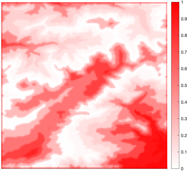
Figure 8: 128$\times$128 original map of environment. Shading of red indicates the probability that a cell is occupied.

5.1 Region-Agnostic Abstraction

In this section, we assume that $p(x)$ is uniform. By changing $\beta$ we obtain a family of solutions, with the leaf node cardinality of the resulting tree returned by the respective algorithm shown in Figure 9.

Figure 9: $\nicefrac{{\lvert\Omega_{T}\rvert}}{{\lvert\Omega_{X}\rvert}}$ vs. $\nicefrac{{\beta}}{{100}}$ for the Greedy and Q-tree search algorithms, $\lvert\Omega_{X}\rvert=16384$.

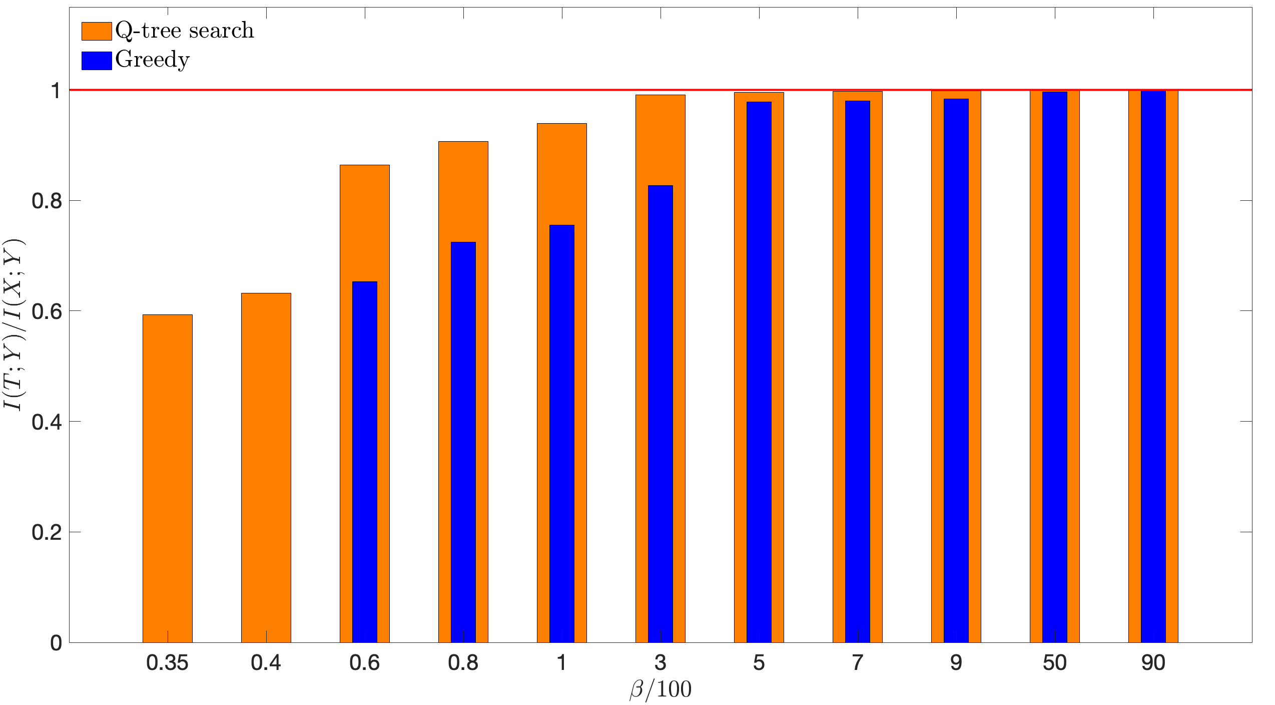
Figure 10: $\nicefrac{{I(T;Y)}}{{I(Y;X)}}$ vs. $\nicefrac{{\beta}}{{100}}$ for the Greedy and Q-tree search algorithms.

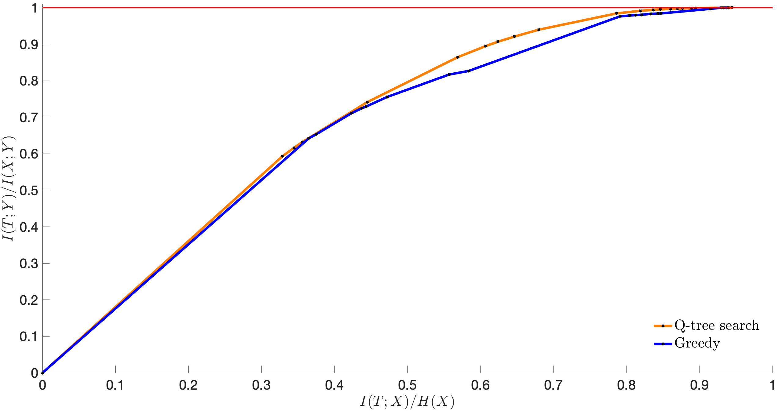
Figure 11: Information plane for Greedy and Q-tree search algorithms.

As seen in Figure 9, the number of leaf nodes of the trees found by both algorithms is increasing with $\beta$. Furthermore, the Q-tree search and Greedy leaf node cardinalities converge as $\beta$ tends toward infinity, as expected. Additionally, as seen in Figure 10, the information contained in the compressed representation $T$ regarding the relevant variable $Y$, given by $I(T;Y)$, approaches the information that the original space $X$ contains about $Y$, quantified by $I(X;Y)$. Note also that $I(T;Y)\leq I(X;Y)$, which follows from the Markov chain $Y\to X\to T$ and the data processing inequality. This encodes the fact that the information contained about the relevant variable $Y$ retained by the abstraction $T$ cannot exceed that given by the original space $X$. Furthermore, from Figure 10, we notice that the Q-tree search algorithm finds solutions that are more informative regarding the relevant variable $Y$ than the Greedy algorithm, indicating that the Greedy algorithm terminates prematurely, and that further improvement is possible for the given $\beta>0$. We also see that the solutions of the Greedy algorithm and of the Q-tree search converge as $\beta$ approaches infinity.

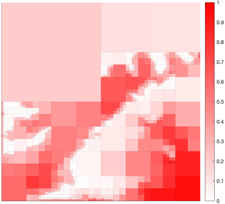
Figure 12: $\beta=50$ representation.

Figure 13: $\beta=100$ representation.

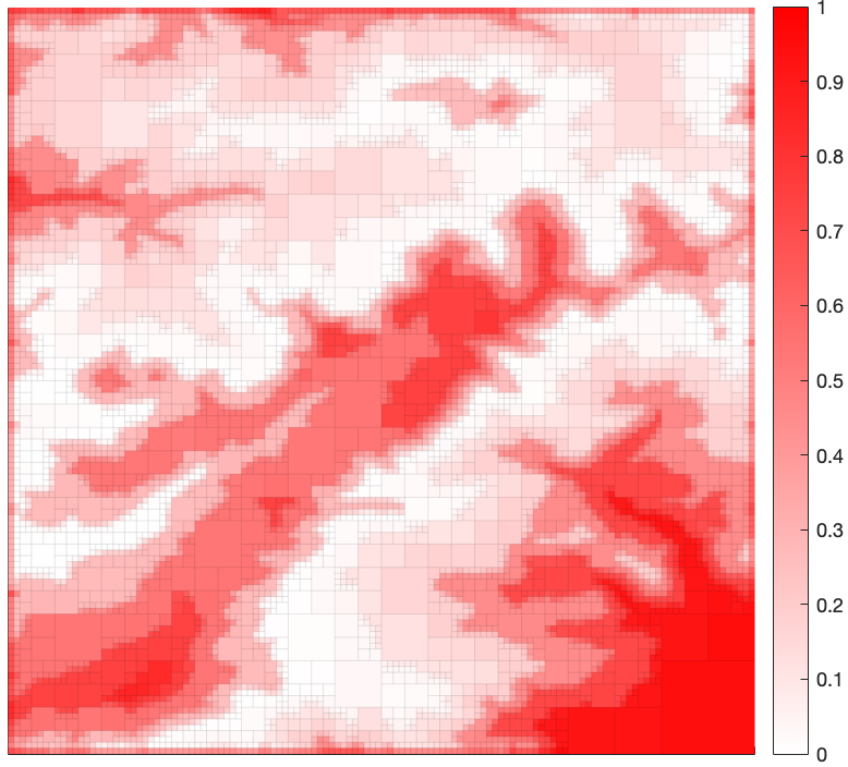
Figure 14: $\beta=400$ representation.

Figure 15: $\beta=15000$ representation.

Shown in Figure 11 is the information plane, where the normalized $I(T;Y)$ is plotted versus the normalized $I(T;X)$. In this way, the information plane displays the amount of relevant information retained in a solution vs. the level of compression of $X$. In viewing this figure, recall that Theorem 4.8 establishes the global optimality of solutions obtained by Q-tree search, and hence no solution above the Q-tree search line is possible in the space $\mathcal{T}^{\mathcal{Q}}$, since this would imply that solutions (trees) encoding more information about $Y$, and for the same level of compression, exist in $\mathcal{T}^{\mathcal{Q}}$.

With this in mind, Figure 11 also corroborates that the Greedy algorithm generally finds solutions that are sub-optimal with respect to $L_{Y}(\cdot;\beta)$, since trees found by the Greedy algorithm retain less information about $Y$ for the same level of compression as the information-plane curve of Greedy lies below that of Q-tree search. Moving along the curve is done by varying $\beta$, with increasing $\beta$ moving the solution to the right in this plane, towards more informative, higher cardinality solutions. We can see from Figure 11 the advantage of utilizing the Q-tree search algorithm, as the Greedy approach arrives at solutions that are sub-optimal compared to those found by the Q-tree search algorithm. A sample of environment depictions for various values of $\beta$ obtained from the Q-tree search algorithm are shown in Figures 13-15. As seen in these figures, the solution returned by the Q-tree search algorithm approaches that of the original space as $\beta\to\infty$, with a spectrum of solutions obtained as $\beta$ is varied. These figures show that areas containing high information content, as specified by $Y$, are refined first while leaving the regions with less information content to be refined at a higher $\beta$.

We see that $\beta$ resembles a sort of a “gain” that can be increased, resulting in progressively more informative solutions of higher cardinality. Thus, once the map is given, changing only the value of $\beta$ gives rise to a variety of solutions of varying resolution. That is, our framework finds the optimal tree $\mathcal{T}_{q^{*}}$ with respect to $L_{Y}(\cdot;\beta)$ without the need to specify pre-defined pruning rules or a host of parameters that define the granularity of the abstraction a priori. Interestingly, $\beta$ plays a similar role in this work as in [18, 22, 23]. Namely, as $\beta\to 0$, highly compressed representations of the space are obtained whereas for large values of $\beta$, we asymptotically approach the original map. Thus, we can view $\beta$ as a “rationality parameter,” analogous to [18, 22, 23], where agents with low $\beta$ are considered to be more resource limited, thus utilizing simpler, lower cardinality representations of the environment.

5.2 Region-Specific Abstraction

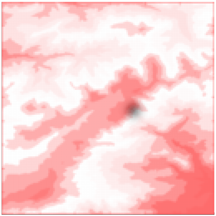
Figure 16: 128$\times$128 original map of environment with overlayed $p(x)$. Shading of red indicates the probability that a cell is occupied by an obstacle, whereas the shade of black indicates cell probability mass under $p(x)$.

In the previous section, we discussed how the Greedy and Q-tree search algorithms can be used to obtain abstractions as a function of $\beta>0$ under the assumption that the distribution $p(x)$ is uniform. We now relax this assumption and discuss the ability to obtain region-specific abstractions in the environment through a non-uniform $p(x)$, without modification to the underlying framework or algorithms as discussed in Section 4.3.

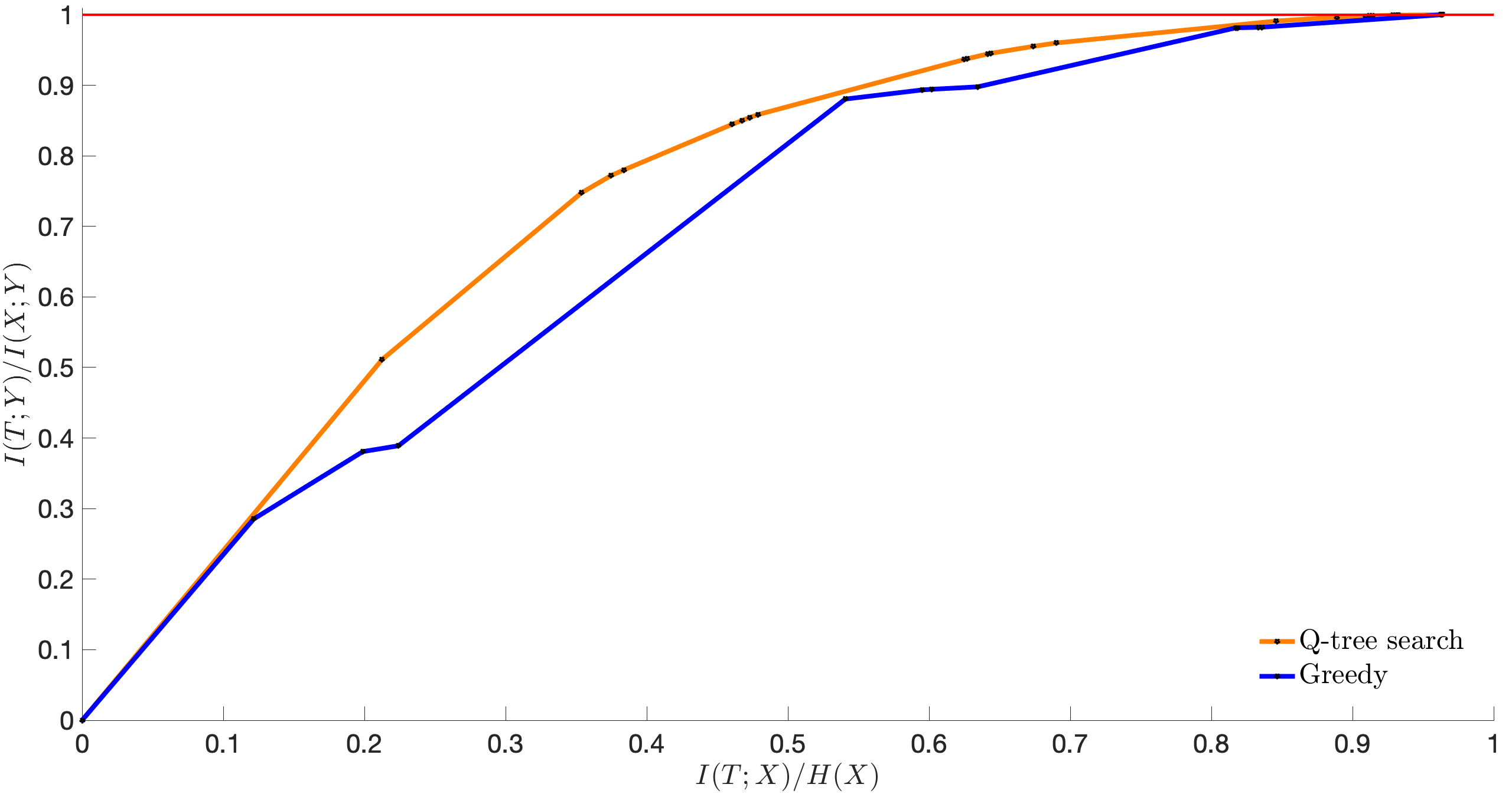
Figure 17: Information plane for Greedy and Q-tree search algorithms, non-uniform $p(x)$.

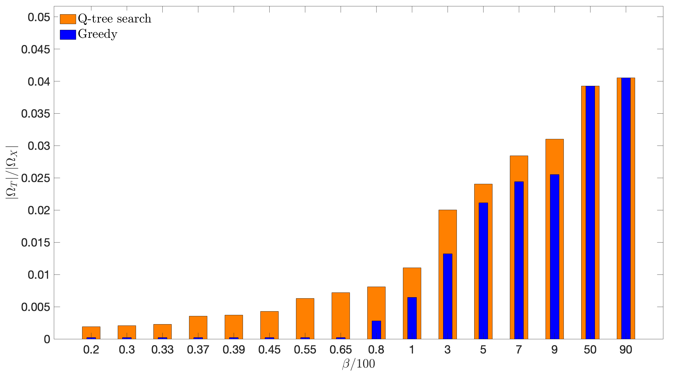
Figure 18: $\nicefrac{{\lvert\Omega_{T}\rvert}}{{\lvert\Omega_{X}\rvert}}$ vs. $\nicefrac{{\beta}}{{100}}$ for Greedy and Q-tree search algorithms, non-uniform $p(x)$. Note y-axis scaling, $\lvert\Omega_{X}\rvert=16384$.

We utilize the same environment as in Figure 8, but with a non-uniform distribution $p(x)$, as shown in Figure 16. In this example, we take $p(x)$ to be a two-dimensional Gaussian distribution with mean $\mu=\left[80,63\right]^{\mbox{\tiny\sf T}}$ and covariance matrix $\Sigma=10I_{2\times 2}$. For comparison, we obtain solutions from both the Greedy and Q-tree search algorithms for a range of $\beta$-values.

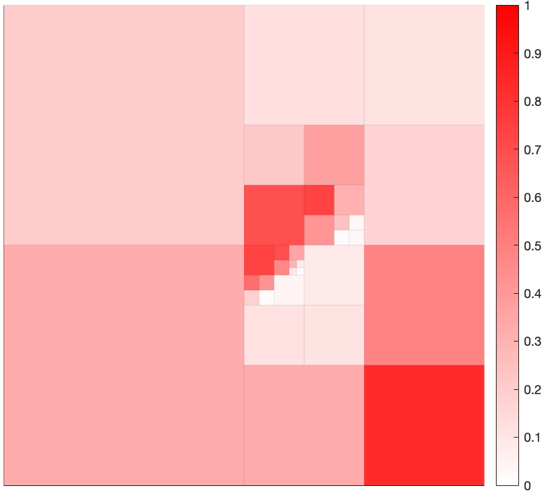
Figure 19: $\beta=25$ representation.

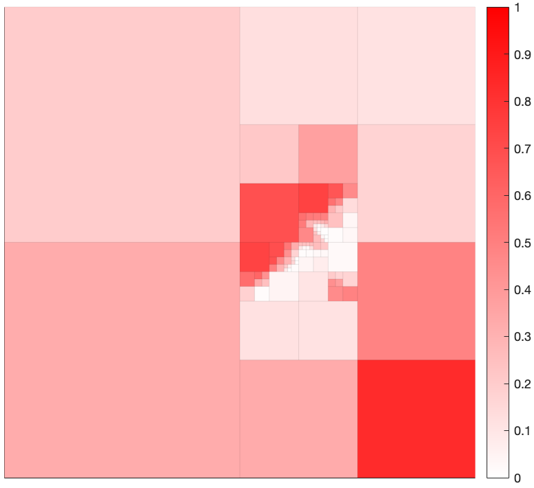
Figure 20: $\beta=55$ representation.

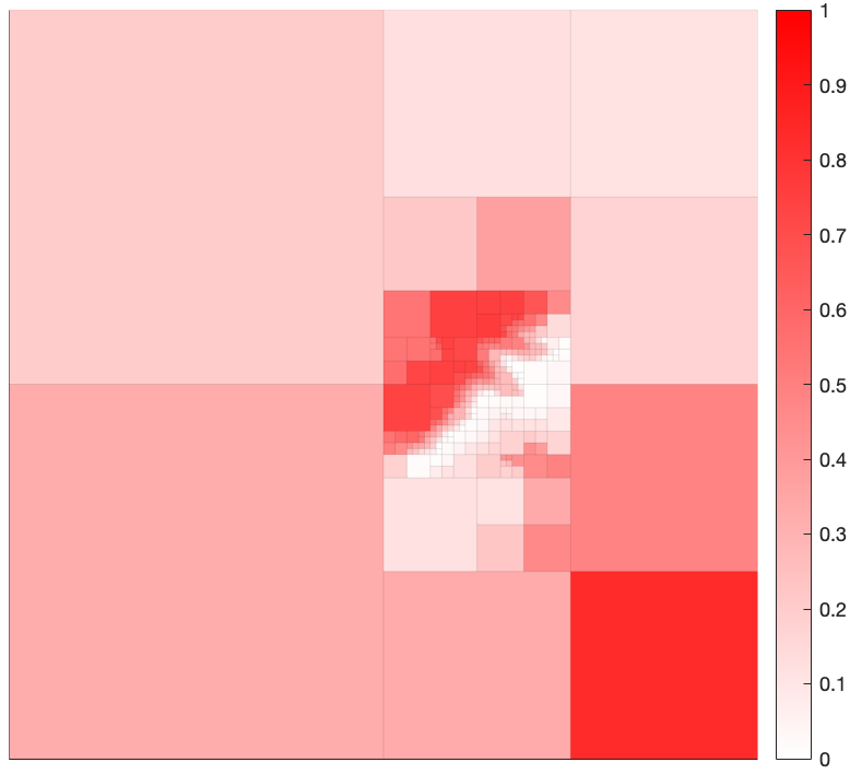
Figure 21: $\beta=200$ representation.

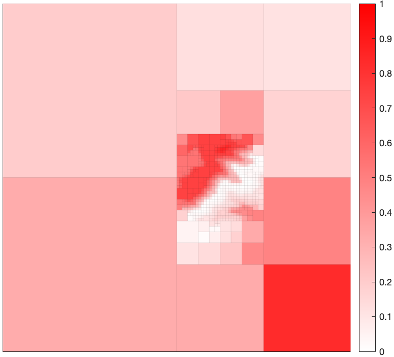
Figure 22: $\beta=15000$ representation.

The information plane is shown in Figure 17 with the cardinality of the resulting tree in Figure 18. We see from Figure 17 that the Greedy algorithm finds solutions that are sub-optimal with respect to Q-tree search, since for a given level of compression ($I(T;X)$), the Greedy algorithm finds solutions that are less informative about $Y$. Figure 18 shows that the Q-tree search algorithm finds solutions that are of higher leaf-node cardinality than those found by Greedy, but that the solutions returned by Q-tree search contain more relevant information. Figures 9 and 18 differ due to the difference in $p(x)$ in the sense that regions with $p(x)=0$ do not contain any information regarding $Y$, as seen by (34) and the subsequent discussion. Finally, visualizations of the resulting solutions obtained from the Q-tree search algorithm are provided in Figures 22-22. These figures corroborate the previous observations, where we can clearly see that the algorithm refines only regions for which $p(x)>0$. Furthermore, the refinement is progressive and of increasing resolution as $\beta\to\infty$.

6 Conclusions

In this paper, we have developed a novel framework for the emergence of abstractions that are not provided to the agent a priori but instead arise as a result of the available agent computational resources. We utilize concepts from information theory, such as the information bottleneck and agglomerative information bottleneck methods to formulate a new optimization problem over the space of trees. The structural properties of the framework were discussed with applications to bounded rationality and information-limited agents. Finally, we propose and analyze two algorithms, which were implemented in order to obtain solutions for a two-dimensional environment.

The importance of this work lies in the development of a framework that allows for the emergence of abstractions in a principled manner. The proposed algorithms demonstrate the utility of the approach, requiring only the specification of a relevant variable that contains the information we wish to retain in the resulting compressed representation. The framework then searches for trees that not only compress the original space, but maximally preserve the information regarding the relevant variable. The results can be utilized in decision-making problems to systematically compress the given state representation or in path-planning algorithms to develop reduced complexity representations of the original planning space.

Appendix

6.1 Proof of Theorem 4.1

Note that

$$\Delta L_{Y}( \mathcal{T}_{q^{i}},\mathcal{T}_{q^{i+1}};\beta)\leq$$

$$\Delta L_{Y}(\mathcal{T}_{q^{i}},\mathcal{T}_{q^{i+1}};\beta)+\sum_{\tau=1}^{n}Q_{Y}(\mathcal{T}_{q^{i+1}},\mathcal{T}_{q_{\tau}^{i+2}};\beta),$$ (35)

since $Q_{Y}(\mathcal{T}_{q^{i+1}},\mathcal{T}_{q_{\tau}^{i+2}};\beta)\geq 0$. In the Greedy algorithm, a node is expanded, adding $\left\{t^{\prime}_{1},\ldots,t^{\prime}_{n}\right\}$ to $\mathcal{N}(\mathcal{T}_{q^{i}})$ to obtain $\mathcal{N}(\mathcal{T}_{q^{i+1}})$, if $\Delta L_{Y}(\mathcal{T}_{q^{i}},\mathcal{T}_{q^{i+1}};\beta)>0$. If $\Delta L_{Y}(\mathcal{T}_{q^{i}},\mathcal{T}_{q^{i+1}};\beta)>0$ then by (6.1) and (26) it follows that

$$0<\Delta L_{Y}(\mathcal{T}_{q^{i}},\mathcal{T}_{q^{i+1}};\beta)+\sum_{\tau=1}^{n}Q_{Y}(\mathcal{T}_{q^{i+1}},\mathcal{T}_{q_{\tau}^{i+2}};\beta )$$

$$=Q_{Y}(\mathcal{T}_{q^{i}},\mathcal{T}_{q^{i+1}};\beta ),$$

and therefore $Q_{Y}(\mathcal{T}_{q^{i}},\mathcal{T}_{q^{i+1}};\beta)>0$. Hence nodes expanded by the Greedy algorithm will also be expanded by Q-tree search. Since the two algorithms are initialized at a common $\mathcal{T}_{q^{0}}\in\mathcal{T}^{\mathcal{Q}}$, it follows that $\mathcal{T}_{q_{\mathrm{G}}^{*}}\subseteq\mathcal{T}_{q_{\mathrm{Q}}^{*}}$.

6.2 Proof of Lemma 4.6

The proof is given by induction. We first establish necessity and sufficiency for some $t\in\mathcal{N}_{\ell-1}(\mathcal{T}_{\mathcal{W}})$, where $\ell>0$ is the maximum depth of $\mathcal{T}_{\mathcal{W}}$.
($\Rightarrow$) Assume $\hat{Q}_{Y}(t;\beta)>0$ for some $t\in\mathcal{N}_{\ell-1}(\mathcal{T}_{\mathcal{W}})$. We thus have

$$0<\hat{Q}_{Y}(t;\beta)=\max\big{\{}\Delta\hat{L}_{Y}(t;\beta)+\sum_{t^{\prime}\in\mathcal{C}(t)}\hat{Q}_{Y}(t^{\prime};\beta);~{}0\big{\}}.$$

Hence,

$$\Delta\hat{L}_{Y}(t;\beta)+\sum_{t^{\prime}\in\mathcal{C}(t)}\hat{Q}_{Y}(t^{\prime};\beta)>0.$$

Since $t\in\mathcal{N}_{\ell-1}(\mathcal{T}_{\mathcal{W}})$ it follows that $t^{\prime}\in\mathcal{C}(t)\subset\mathcal{N}_{\text{leaf}}(\mathcal{T}_{\mathcal{W}})$ and thus $\hat{Q}_{Y}(t^{\prime};\beta)=0$, which implies that $\Delta\hat{L}_{Y}(t;\beta)=\hat{Q}_{Y}(t;\beta)>0$. Now consider the tree $\mathcal{T}_{q}\in\mathcal{T}^{\mathcal{Q}}$ such that $\mathcal{N}_{\text{leaf}}(\mathcal{T}_{q(t)})=\mathcal{C}(t)$. Then, for the subtree $\mathcal{T}_{q(t)}\subseteq\mathcal{T}_{\mathcal{W}}$

$$\sum_{z\in\mathcal{N}_{\text{int}}(\mathcal{T}_{q(t)})}\Delta\hat{L}_{Y}(z;\beta)=\Delta\hat{L}_{Y}(t;\beta)>0.$$

($\Leftarrow$) Assume there exists a tree $\mathcal{T}_{q}\in\mathcal{T}^{\mathcal{Q}}$ such that

$$\sum_{z\in\mathcal{N}_{\text{int}}(\mathcal{T}_{q(t)})}\Delta\hat{L}_{Y}(z;\beta)>0.$$

Note that, since $t\in\mathcal{N}_{\ell-1}(\mathcal{T}_{\mathcal{W}})$ then $\mathcal{N}(\mathcal{T}_{q(t)})=\left\{t\right\}\cup\mathcal{C}(t)$, with $\mathcal{N}_{\text{int}}(\mathcal{T}_{q(t)})=\left\{t\right\}$ and $\mathcal{N}_{\text{leaf}}(\mathcal{T}_{q(t)})=\mathcal{C}(t)\subset\mathcal{N}_{\text{leaf}}(\mathcal{T}_{\mathcal{W}})$. Therefore,

$$0<\sum_{z\in\mathcal{N}_{\text{int}}(\mathcal{T}_{q(t)})}\Delta\hat{L}_{Y}(z;\beta)=\Delta\hat{L}_{Y}(t;\beta),$$

and

$$\hat{Q}_{Y}(t;\beta) =\max\big{\{}\Delta\hat{L}_{Y}(t;\beta)+\sum_{t^{\prime}\in\mathcal{C}(t)}\hat{Q}_{Y}(t^{\prime};\beta),~{}0\big{\}},$$

$$=\max\big{\{}\Delta\hat{L}_{Y}(t;\beta),~{}0\big{\}},$$

$$=\Delta\hat{L}_{Y}(t;\beta)>0.$$

Furthermore, for the tree $\mathcal{T}_{q}$ we have $\sum_{z\in\mathcal{N}_{\text{int}}(\mathcal{T}_{q(t)})}\Delta\hat{L}_{Y}(z;\beta)=\hat{Q}_{Y}(t;\beta)$ and since $t\in\mathcal{N}_{\ell-1}(\mathcal{T}_{\mathcal{W}})$, for any other tree $\mathcal{T}_{\tilde{q}}$ such that $\mathcal{T}_{\tilde{q}(t)}\neq\mathcal{T}_{q(t)}$, it holds that $\mathcal{N}_{\text{int}}({\mathcal{T}_{\tilde{q}(t)}})=\emptyset$, which implies that $\sum_{z\in\mathcal{N}_{\text{int}}(\mathcal{T}_{\tilde{q}(t)})}\Delta\hat{L}_{Y}(z;\beta)=0\leq\hat{Q}_{Y}(t;\beta).$ Thus, the lemma is true for all nodes $t\in\mathcal{N}_{\ell-1}(\mathcal{T}_{\mathcal{W}})$.

We now establish necessity and sufficiency for all $k\in\left\{1,\ldots,\ell-1\right\}$. To this end, assume that for some $k\in\left\{1,\ldots,\ell-1\right\}$ and any $t^{\prime}\in\mathcal{N}_{k}(\mathcal{T}_{\mathcal{W}})$, $\hat{Q}_{Y}(t^{\prime};\beta)>0$ if and only if there exists a tree $\mathcal{T}_{q}\in\mathcal{T}^{\mathcal{Q}}$ such that $\sum_{z\in\mathcal{N}_{\text{int}}(\mathcal{T}_{q(t^{\prime})})}\Delta\hat{L}_{Y}(z;\beta)>0$. Furthermore, if $\hat{Q}_{Y}(t^{\prime};\beta)>0$ then there exists a tree $\mathcal{T}_{q^{*}}\in\mathcal{T}^{\mathcal{Q}}$ such that $\sum_{z\in\mathcal{N}_{\text{int}}(\mathcal{T}_{q^{*}(t^{\prime})})}\Delta\hat{L}_{Y}(z;\beta)=\hat{Q}_{Y}(t^{\prime};\beta)$, and for all other trees $\mathcal{T}_{\tilde{q}}\in\mathcal{T}^{\mathcal{Q}}$ with $t^{\prime}\in\mathcal{N}(\mathcal{T}_{\tilde{q}})$ and $\mathcal{T}_{\tilde{q}(t^{\prime})}\neq\mathcal{T}_{q^{*}(t^{\prime})}$, $\sum_{z\in\mathcal{N}_{\text{int}}(\mathcal{T}_{\tilde{q}(t^{\prime})})}\Delta\hat{L}_{Y}(z;\beta)\leq\hat{Q}_{Y}(t^{\prime};\beta)$. Using this hypothesis, we prove that the lemma also holds for all $t\in\mathcal{N}_{k-1}(\mathcal{T}_{\mathcal{W}})$.

$\left(\Rightarrow\right)$ Consider $t\in\mathcal{N}_{k-1}(\mathcal{T}_{\mathcal{W}})$ and assume that $\hat{Q}_{Y}(t;\beta)>0$. Define the set

$$\mathcal{S}=\left\{t^{\prime}\in\mathcal{C}(t):\hat{Q}_{Y}(t^{\prime};\beta)>0\right\}\subset\mathcal{N}_{k}(\mathcal{T}_{\mathcal{W}}).$$

If $\mathcal{S}=\emptyset$ then from Definition 4.5, $0<\hat{Q}_{Y}(t;\beta)=\max\{\Delta\hat{L}_{Y}(t;\beta),0\}$, and therefore $\hat{Q}_{Y}(t;\beta)=\Delta\hat{L}_{Y}(t;\beta)>0$. Now, consider any tree $\mathcal{T}_{q}\in\mathcal{T}^{\mathcal{Q}}$ such that $\mathcal{T}_{q(t)}$ has node set $\mathcal{N}(\mathcal{T}_{q(t)})=\left\{t\right\}\cup\mathcal{C}(t)$. Note that $\mathcal{N}_{\text{int}}(\mathcal{T}_{q(t)})=\left\{t\right\}$ and $\mathcal{N}_{\text{leaf}}(\mathcal{T}_{q(t)})=\mathcal{C}(t)$. Thus, for the subtree $\mathcal{T}_{q(t)}$,

$$\sum_{z\in\mathcal{N}_{\text{int}}(\mathcal{T}_{q(t)})}\Delta\hat{L}_{Y}(z;\beta)=\Delta\hat{L}_{Y}(t;\beta)=\hat{Q}_{Y}(t;\beta).$$

Therefore $\hat{Q}_{Y}(t;\beta)>0$ implies that there exists a tree $\mathcal{T}_{q}\in\mathcal{T}^{\mathcal{Q}}$ such that $\sum_{z\in\mathcal{N}_{\text{int}}(\mathcal{T}_{q(t)})}\Delta\hat{L}_{Y}(z;\beta)>0$.

Now consider $\mathcal{S}\neq\emptyset$. By hypothesis, there exists a tree $\mathcal{T}_{q^{*}}\in\mathcal{T}^{\mathcal{Q}}$ such that

$$\sum_{z\in\mathcal{N}_{\text{int}}(\mathcal{T}_{q^{*}(t^{\prime})})}\Delta\hat{L}_{Y}(z;\beta)=\hat{Q}_{Y}(t^{\prime};\beta),~{}~{}\forall t^{\prime}\in\mathcal{S}.$$

Consider a tree $\mathcal{T}_{q}\in\mathcal{T}^{\mathcal{Q}}$ such that $\mathcal{T}_{q(t)}$ has the properties

$$\mathcal{N}_{\text{int}}(\mathcal{T}_{q(t)})=\left\{t\right\}\bigcup\limits_{t^{\prime}\in\mathcal{S}}\mathcal{N}_{\text{int}}(\mathcal{T}_{q^{*}(t^{\prime})}),$$

and

$$\mathcal{N}_{\text{leaf}}(\mathcal{T}_{q(t)})=\left(\mathcal{C}(t)\setminus\mathcal{S}\right)\bigcup\limits_{t^{\prime}\in\mathcal{S}}\mathcal{N}_{\text{leaf}}(\mathcal{T}_{q^{*}(t^{\prime})}).$$

Therefore, using the fact that $\sum_{z\in\mathcal{N}_{\text{int}}(\mathcal{T}_{q^{*}(t^{\prime})})}\Delta\hat{L}_{Y}(z;\beta)=\hat{Q}_{Y}(t^{\prime};\beta)$, for all $t^{\prime}\in\mathcal{S}$, we have

$$\sum_{z\in\mathcal{N}_{\text{int}}(\mathcal{T}_{q(t)})}\Delta\hat{L}_{Y}(z;\beta) =\Delta\hat{L}_{Y}(t;\beta)+\sum_{t^{\prime}\in\mathcal{S}}\sum_{z\in\mathcal{N}_{\text{int}}(\mathcal{T}_{q^{*}(t^{\prime})})}\Delta\hat{L}_{Y}(z;\beta),$$

$$=\Delta\hat{L}_{Y}(t;\beta)+\sum_{t^{\prime}\in\mathcal{S}}\hat{Q}_{Y}(t^{\prime};\beta).$$

Also note that $\hat{Q}_{Y}(t^{\prime};\beta)=0$ for all $t^{\prime}\in\mathcal{C}(t)\setminus\mathcal{S}$ and hence,

$$\sum_{z\in\mathcal{N}_{\text{int}}(\mathcal{T}_{q(t)})} \Delta\hat{L}_{Y}(z;\beta)=\Delta\hat{L}_{Y}(t;\beta)+\sum_{t^{\prime}\in\mathcal{S}}\hat{Q}_{Y}(t^{\prime};\beta)+\sum_{t^{\prime}\in\left\{\mathcal{C}(t)\setminus\mathcal{S}\right\}}\hat{Q}_{Y}(t^{\prime};\beta).$$

Furthermore, note that from Definition 4.5, if $\hat{Q}_{Y}(t;\beta)>0$ then

$$\hat{Q}_{Y}(t;\beta)=\Delta\hat{L}_{Y}(t;\beta)+\sum_{t^{\prime}\in\mathcal{C}(t)}\hat{Q}_{Y}(t^{\prime};\beta),$$

and thus,

$$\sum_{z\in\mathcal{N}_{\text{int}}(\mathcal{T}_{q(t)})}\Delta\hat{L}_{Y}(z;\beta)=\hat{Q}_{Y}(t;\beta)>0.$$

Therefore, it follows that if $\hat{Q}_{Y}(t;\beta)>0$, there exists a tree such that $\sum_{z\in\mathcal{N}_{\text{int}}(\mathcal{T}_{q(t)})}\Delta\hat{L}_{Y}(z;\beta)>0$ and $\sum_{z\in\mathcal{N}_{\text{int}}(\mathcal{T}_{q(t)})}\Delta\hat{L}_{Y}(z;\beta)$ $=\hat{Q}_{Y}(t;\beta)$.

Furthermore, consider any $\mathcal{T}_{\tilde{q}}\in\mathcal{T}^{\mathcal{Q}}$ such that $\mathcal{T}_{\tilde{q}(t)}\neq\mathcal{T}_{q(t)}$. Then

$$\sum_{z\in\mathcal{N}_{\text{int}}(\mathcal{T}_{\tilde{q}(t)})}\Delta\hat{L}_{Y}(z;\beta)=\Delta\hat{L}_{Y}(t;\beta)+\sum_{t^{\prime}\in\left\{\mathcal{C}(t)\cap\mathcal{N}_{\text{int}}(\mathcal{T}_{\tilde{q}(t)})\right\}}\left(\sum_{z\in\mathcal{N}_{\text{int}}(\mathcal{T}_{\tilde{q}(t^{\prime})})}\Delta\hat{L}_{Y}(z;\beta)\right).$$

Note that $t^{\prime}\in\mathcal{N}_{k}(\mathcal{T}_{\mathcal{W}})$ and that

$$\sum_{z\in\mathcal{N}_{\text{int}}(\mathcal{T}_{\tilde{q}(t^{\prime})})}\Delta\hat{L}_{Y}(z;\beta)\leq\hat{Q}_{Y}(t^{\prime};\beta).$$

Consequently,

$$\sum_{z\in\mathcal{N}_{\text{int}}(\mathcal{T}_{\tilde{q}(t)})}\Delta\hat{L}_{Y}(z;\beta) \leq\Delta\hat{L}_{Y}(t;\beta)+\sum_{t^{\prime}\in\left\{\mathcal{C}(t)\cap\mathcal{N}_{\text{int}}(\mathcal{T}_{\tilde{q}(t)})\right\}}\hat{Q}_{Y}(t^{\prime};\beta),$$

$$\leq\Delta\hat{L}_{Y}(t;\beta)+\sum_{t^{\prime}\in\mathcal{C}(t)}\hat{Q}_{Y}(t^{\prime};\beta),$$

$$=\hat{Q}_{Y}(t;\beta).$$

$\left(\Leftarrow\right)$ Let $t\in\mathcal{N}_{k-1}(\mathcal{T}_{\mathcal{W}})$ and assume that there exists a tree $\mathcal{T}_{q}\in\mathcal{T}^{\mathcal{Q}}$ such that

$$\sum_{z\in\mathcal{N}_{\text{int}}(\mathcal{T}_{q(t)})}\Delta\hat{L}_{Y}(z;\beta)>0,$$

and consider any $t^{\prime}\in\mathcal{N}_{\text{int}}(\mathcal{T}_{q(t)})\cap\mathcal{C}(t)\subset\mathcal{N}_{k}(\mathcal{T}_{\mathcal{W}})$. From the hypothesis we have that

$$\sum_{z\in\mathcal{N}_{\text{int}}(\mathcal{T}_{q(t^{\prime})})}\Delta\hat{L}_{Y}(z;\beta)\leq\hat{Q}_{Y}(t^{\prime};\beta).$$

Therefore,

$$\sum_{z\in\mathcal{N}_{\text{int}}(\mathcal{T}_{q(t)})}\Delta\hat{L}_{Y}(z;\beta)=\Delta\hat{L}_{Y}(t;\beta)+\sum_{t^{\prime}\in\left\{\mathcal{C}(t)\cap\mathcal{N}_{\text{int}}(\mathcal{T}_{q(t)})\right\}}\left(\sum_{z\in\mathcal{N}_{\text{int}}(\mathcal{T}_{q(t^{\prime})})}\Delta\hat{L}_{Y}(z;\beta)\right),$$

which yields

$$0< \sum_{z\in\mathcal{N}_{\text{int}}(\mathcal{T}_{q(t)})}\Delta\hat{L}_{Y}(z;\beta)\leq\Delta\hat{L}_{Y}(t;\beta)+\sum_{t^{\prime}\in\left\{\mathcal{C}(t)\cap\mathcal{N}_{\text{int}}(\mathcal{T}_{q(t)})\right\}}\hat{Q}_{Y}(t^{\prime};\beta)+\underbrace{\sum_{t^{\prime}\in\left\{\mathcal{C}(t)\setminus\mathcal{N}_{\text{int}}(\mathcal{T}_{q(t)})\right\}}\hat{Q}_{Y}(t^{\prime};\beta)}_{\text{$\geq 0$}}.$$

Hence,

$$0<\Delta\hat{L}_{Y}(t;\beta)+\sum_{t^{\prime}\in\mathcal{C}(t)}\hat{Q}_{Y}(t^{\prime};\beta)\leq\hat{Q}_{Y}(t;\beta).$$

Therefore, the existence of a tree $\mathcal{T}_{q}\in\mathcal{T}^{\mathcal{Q}}$ with $\sum_{z\in\mathcal{N}_{\text{int}}(\mathcal{T}_{q(t)})}\Delta\hat{L}_{Y}(z;\beta)>0$ where $t\in\mathcal{N}_{k-1}(\mathcal{T}_{\mathcal{W}})$ implies $\hat{Q}_{Y}(t;\beta)>0$.

Thus, we have shown that the lemma holds for $k-1$ and for all $t\in\mathcal{N}_{k-1}(\mathcal{T}_{\mathcal{W}})$.

6.3 Proof of Lemma 4.7

Let $t\in\mathcal{N}(\mathcal{T}_{\mathcal{W}})$ be any node such that $t\in\mathcal{N}_{\text{leaf}}(\mathcal{T}_{q^{\prime}})\cap\mathcal{N}_{\text{int}}(\mathcal{T}_{q^{*}})$, where $\mathcal{T}_{q^{\prime}}\subset\mathcal{T}_{q^{*}}$. Note that $\hat{Q}_{Y}(n;\beta)>0$ for all $n\in\mathcal{N}_{\text{int}}(\mathcal{T}_{q^{*}(t)})$ and $\hat{Q}_{Y}(n;\beta)=0$ for all $n\in\mathcal{N}_{\text{leaf}}(\mathcal{T}_{q^{*}(t)})$, which follows from the design of the Q-tree search algorithm. Thus, we have that

$$\sum_{z\in\mathcal{N}_{\text{int}}(\mathcal{T}_{q^{*}(t)})}\Delta\hat{L}_{Y}(z;\beta)=\hat{Q}_{Y}(t;\beta)>0,$$

which holds for all $t\in\mathcal{N}_{\text{leaf}}(\mathcal{T}_{q^{\prime}})\cap\mathcal{N}_{\text{int}}(\mathcal{T}_{q^{*}})$. Furthermore, using (33),

$$L_{Y}(\mathcal{T}_{q^{\prime}};\beta)+\sum_{t\in\left\{\mathcal{N}_{\text{leaf}}(\mathcal{T}_{q^{\prime}})\cap\mathcal{N}_{\text{int}}(\mathcal{T}_{q^{*}})\right\}} \sum_{z\in\mathcal{N}_{\text{int}}(\mathcal{T}_{q^{*}(t)})}\Delta\hat{L}_{Y}(z;\beta)=L_{Y}(\mathcal{T}_{q^{*}};\beta).$$

The above is equivalent to

$$L_{Y}(\mathcal{T}_{q^{\prime}};\beta)+\sum_{t\in\left\{\mathcal{N}_{\text{leaf}}(\mathcal{T}_{q^{\prime}})\cap\mathcal{N}_{\text{int}}(\mathcal{T}_{q^{*}})\right\}}\hat{Q}_{Y}(t;\beta)=L_{Y}(\mathcal{T}_{q^{*}};\beta).$$

Lastly, it is known that Q-tree search did not terminate at $\mathcal{T}_{q^{\prime}}$. Thus, $\sum_{t\in\left\{\mathcal{N}_{\text{leaf}}(\mathcal{T}_{q^{\prime}})\cap\mathcal{N}_{\text{int}}(\mathcal{T}_{q^{*}})\right\}}\hat{Q}_{Y}(t;\beta)>0$, where $N_{\text{leaf}}(\mathcal{T}_{q^{\prime}})\cap\mathcal{N}_{\text{int}}(\mathcal{T}_{q^{*}})\neq\emptyset$ if $\mathcal{T}_{q^{\prime}}\neq\mathcal{T}_{q^{*}}$, and therefore

$$L_{Y}(\mathcal{T}_{q^{\prime}};\beta)<L_{Y}(\mathcal{T}_{q^{*}};\beta).$$

6.4 Proof of Theorem 4.8

Let $t\in\mathcal{N}_{\text{int}}(\mathcal{T}_{\tilde{q}})$ and consider the tree $\mathcal{T}_{\bar{q}}\in\mathcal{T}^{\mathcal{Q}}$ with node set $\mathcal{N}(\mathcal{T}_{\bar{q}})=\{t\}\cup\mathcal{N}(\mathcal{T}_{\tilde{q}})\setminus\mathcal{N}(\mathcal{T}_{\tilde{q}(t)})$. We have from (33) that

$$L_{Y}(\mathcal{T}_{\bar{q}};\beta)=\sum_{z\in\left\{\mathcal{N}_{\text{int}}(\mathcal{T}_{\tilde{q}})\setminus\mathcal{N}_{\text{int}}(\mathcal{T}_{\tilde{q}(t)})\right\}}\Delta\hat{L}_{Y}(z;\beta).$$

From the above expression and (21) and (30), we have

$$L_{Y}(\mathcal{T}_{\tilde{q}};\beta)=L_{Y}(\mathcal{T}_{\bar{q}};\beta)+\sum_{z\in{\mathcal{N}}_{\text{int}}(\mathcal{T}_{\tilde{q}(t)})}\Delta\hat{L}_{Y}(z;\beta).$$

Since $\mathcal{T}_{\tilde{q}}$ is minimal, for any subtree $\mathcal{T}_{\bar{q}}$ we have $L_{Y}(\mathcal{T}_{\bar{q}};\beta)<L_{Y}(\mathcal{T}_{\tilde{q}};\beta)$, and therefore

$$\sum_{z\in{\mathcal{N}}_{\text{int}}(\mathcal{T}_{\tilde{q}(t)})}\Delta\hat{L}_{Y}(z;\beta)>0,~{}~{}~{}\forall t\in\mathcal{N}_{\text{int}}(\mathcal{T}_{\tilde{q}}).$$

Hence, from Lemma 4.6, $\hat{Q}_{Y}(t;\beta)>0$ for all $t\in\mathcal{N}_{\text{int}}(\mathcal{T}_{\tilde{q}})$. Thus, all nodes in $\mathcal{N}_{\text{int}}(\mathcal{T}_{\tilde{q}})$ are expanded in $\mathcal{T}_{q^{*}}$, which implies that $\mathcal{T}_{q^{*}}\supseteq\mathcal{T}_{\tilde{q}}$. Then, either $\mathcal{T}_{q^{*}}=\mathcal{T}_{\tilde{q}}$, which implies $L_{Y}(\mathcal{T}_{\tilde{q}};\beta)=L_{Y}(\mathcal{T}_{q^{*}};\beta)$, or $\mathcal{T}_{q^{*}}\supset\mathcal{T}_{\tilde{q}}$, which, from Lemma 4.7, implies that $L_{Y}(\mathcal{T}_{\tilde{q}};\beta)<L_{Y}(\mathcal{T}_{q^{*}};\beta)$. However, since $\mathcal{T}_{\tilde{q}}$ is optimal, we have $L_{Y}(\mathcal{T}_{\tilde{q}};\beta)\geq L_{Y}(\mathcal{T}_{q^{*}};\beta)$, leading to a contradiction. Thus, $\mathcal{T}_{q^{*}}=\mathcal{T}_{\tilde{q}}$ and consequently $L_{Y}(\mathcal{T}_{\tilde{q}};\beta)=L_{Y}(\mathcal{T}_{q^{*}};\beta)$.

6.5 Proof of Proposition 4.9

Assume $\beta>0$, $t\in\mathcal{N}_{\text{int}}(\mathcal{T}_{\mathcal{W}})$ and $p(x)={\varepsilon}/{N}$ for all $x\in\mathcal{N}_{\text{leaf}}(\mathcal{T}_{\mathcal{W}(t)})$ with $N=\lvert\mathcal{N}_{\text{leaf}}(\mathcal{T}_{\mathcal{W}(t)})\rvert$. By (24) and Definition 4.4, we have

$$\Delta\hat{L}(t;\beta)=p(t)\left[\mathrm{JS}_{\Pi}(p(y|t^{\prime}_{1}),\ldots,p(y|t^{\prime}_{\lvert\mathcal{C}(t)\rvert}))-\frac{1}{\beta}H(\Pi)\right],$$

where, without loss of generality, $\left\{t^{\prime}_{1},\ldots,t^{\prime}_{\lvert\mathcal{C}(t)\rvert}\right\}=\mathcal{C}(t)$. Moreover, since $p(t|x)$ is deterministic,

$$p(t)=\sum_{x\in\mathcal{N}_{\text{leaf}}(\mathcal{T}_{\mathcal{W}})}p(t|x)p(x)=\sum_{x\in\mathcal{N}_{\text{leaf}}(\mathcal{T}_{\mathcal{W}(t)})}p(x)=\varepsilon,$$

and since $p(x)={\varepsilon}/{N}$ for all $x\in\mathcal{N}_{\text{leaf}}(\mathcal{T}_{\mathcal{W}(t)})$, it follows that

$$p(t^{\prime})=\frac{\varepsilon}{\lvert\mathcal{C}(t)\rvert},\quad t^{\prime}\in\mathcal{C}(t).$$

Consequently,

$$\Pi=\left\{\frac{p(t^{\prime}_{1})}{p(t)},\ldots,\frac{p(t^{\prime}_{\lvert\mathcal{C}(t)\rvert})}{p(t)}\right\}=\left\{\frac{1}{\lvert\mathcal{C}(t)\rvert},\ldots,\frac{1}{\lvert\mathcal{C}(t)\rvert}\right\},$$

and therefore,

$$H(\Pi)=\log\lvert\mathcal{C}(t)\rvert.$$ (36)

Now define

$$a_{t^{\prime}}(y)\triangleq\sum_{x\in\mathcal{N}_{\text{leaf}}\left(\mathcal{T}_{\mathcal{W}(t^{\prime})}\right)}p(x,y),$$

and

$$a_{t}(y)\triangleq\sum_{x\in\mathcal{N}_{\text{leaf}}\left(\mathcal{T}_{\mathcal{W}(t)}\right)}p(x,y),$$

where $y\in\Omega_{Y}$ and $t^{\prime}\in\mathcal{C}(t)$. Thus, from the definition of $a_{t^{\prime}}(y)$ and $a_{t}(y)$,

$$\sum_{y}a_{t^{\prime}}(y)=\frac{\varepsilon}{\lvert\mathcal{C}(t)\rvert},$$ (37)

and

$$\sum_{y}a_{t}(y)=\varepsilon,$$

for all $t^{\prime}\in\mathcal{C}(t)$. Since $\mathcal{N}_{\text{leaf}}(\mathcal{T}_{\mathcal{W}(t^{\prime})})\subseteq\mathcal{N}_{\text{leaf}}(\mathcal{T}_{\mathcal{W}(t)})$, it follows that $0\leq a_{t^{\prime}}(y)\leq a_{t}(y)\leq\varepsilon$. Thus, for $t^{\prime}\in\mathcal{C}(t)$ we have, from the definition of the KL-divergence,

$$\mathrm{D}_{\mathrm{KL}}(p(y|t^{\prime}),p(y|t))=\sum_{y}p(y|t^{\prime})\log\frac{p(y|t^{\prime})}{p(y|t)},$$

where

$$p(y|t)=\frac{1}{p(t)}\sum_{x\in\mathcal{N}_{\text{leaf}(\mathcal{T}_{\mathcal{W}(t)})}}p(x,y)=\frac{1}{\varepsilon}a_{t}(y),$$

and similarly,

$$p(y|t^{\prime})=\frac{1}{p(t^{\prime})}\sum_{x\in\mathcal{N}_{\text{leaf}(\mathcal{T}_{\mathcal{W}(t^{\prime})})}}p(x,y)=\frac{\lvert\mathcal{C}(t)\rvert}{\varepsilon}a_{t^{\prime}}(y).$$

Hence,

$$\mathrm{D}_{\mathrm{KL}}(p(y|t {}^{\prime}),p(y|t))=\sum_{y}p(y|t^{\prime})\log\frac{\lvert\mathcal{C}(t)\rvert a_{t^{\prime}}(y)}{a_{t}(y)},$$

$$=\log\lvert\mathcal{C}(t)\rvert+\sum_{y}p(y|t^{\prime})\log\frac{a_{t^{\prime}}(y)}{a_{t}(y)},$$

$$=\log\lvert\mathcal{C}(t)\rvert+\frac{\lvert\mathcal{C}(t)\rvert}{\varepsilon}\sum_{y}a_{t^{\prime}}(y)\log\frac{a_{t^{\prime}}(y)}{a_{t}(y)}.$$ (38)

Since $0\leq a_{t^{\prime}}(y)\leq a_{t}(y)$ for all $y\in\Omega_{Y}$ we have from (37) and (38) that

$$\frac{\lvert\mathcal{C}(t)\rvert}{\varepsilon}\sum_{y}a_{t^{\prime}}(y)\log\frac{a_{t^{\prime}}(y)}{a_{t}(y)} \leq\frac{\lvert\mathcal{C}(t)\rvert}{\varepsilon}\sum_{y}a_{t^{\prime}}(y)\log\frac{a_{t}(y)}{a_{t}(y)},$$

$$=\frac{\lvert\mathcal{C}(t)\rvert}{\varepsilon}\log\left(1\right)\sum_{y}a_{t^{\prime}}(y),$$

$$=0.$$

Thus, from the previous expression, along with (38), it follows that

$$0\leq\mathrm{D}_{\mathrm{KL}}(p(y|t^{\prime}),p(y|t))\leq\log\lvert\mathcal{C}(t)\rvert,~{}~{}~{}\forall t^{\prime}\in\mathcal{C}(t).$$ (39)

Using (39) and the definition of JS-divergence, we see that

$$\mathrm{JS}_{\Pi}(p(y|t^{\prime}_{1}),\ldots,p(y|t^{\prime}_{\lvert\mathcal{C}(t)\rvert}) =\sum_{i=1}^{\lvert\mathcal{C}(t)\rvert}\Pi(i)\mathrm{D}_{\mathrm{KL}}(p(y|t^{\prime}_{i}),p(y|t)),$$

$$\leq\log\lvert\mathcal{C}(t)\rvert.$$

Therefore, from the non-negativity of the JS-divergence as well as (36) and (39) we have,

$$-\frac{1}{\beta}\varepsilon\log\lvert\mathcal{C}(t)\rvert\leq p(t)\big{[}\mathrm{JS}_{\Pi}( p(y|t^{\prime}_{1}),\ldots,p(y|t^{\prime}_{\lvert\mathcal{C}(t)\rvert}))-\frac{1}{\beta}H(\Pi)\big{]}\leq\frac{\beta-1}{\beta}\varepsilon\log\lvert\mathcal{C}(t)\rvert.$$

Now taking the limit as $\varepsilon\to 0^{+}$ yields $\lim_{\varepsilon\to 0^{+}}\Delta\hat{L}(t;\beta)=0$ for all $\beta>0$.

References

- [1] T. M. Cover and J. A. Thomas, Elements of Information Theory, 2nd, Ed. John Wiley & Sons, 2006.
- [2] S. Behnke, “Local multiresolution path planning,” Lecture Notes in Artificial Intelligence, vol. 3020, no. 1, pp. 332–343, 2004.
- [3] D. P. Bertsekas, Dynamic Programming and Optimal Control, 4th ed. Athena Scientific, 2012, vol. 2.
- [4] M. M. Botvinick, “Hierarchical reinforcement learning and decision making,” Current Opinion in Neurobiology, vol. 22, pp. 956–962, June 2012.
- [5] F. Hauer, A. Kundu, J. M. Rehg, and P. Tsiotras, “Multi-scale perception and path planning on probabilistic obstacle maps,” in IEEE International Conference on Robotics and Automation, Seattle, WA, May 26-30 2015, pp. 4210–4215.
- [6] F. Hauer and P. Tsiotras, “Reduced complexity multi-scale path-planning on probabilitic maps,” in IEEE Conference on Robotics and Automation, Stockholm, Sweden, 16-21 May 2016, pp. 83–88.
- [7] S. Kambhampati and L. S. Davis, “Multiresolution path planning for mobile robots,” IEEE Journal of Robotics and Automation, vol. RA-2, no. 3, pp. 135–145, September 1986.
- [8] G. K. Kraetzschmar, G. P. Gassull, and K. Uhl, “Probabilistic quadtrees for variable-resolution mapping of large environments,” IFAC Proceedings Volumes, vol. 37, no. 8, pp. 675–680, July 2004.
- [9] R. V. Cowlagi and P. Tsiotras, “Multiresolution path planning with wavelets: A local replanning approach,” in American Control Conference, Seattle, WA, June 11-13 2008, pp. 1220–1225.
- [10] ——, “Multi-resolution path planning: Theoretical analysis, efficient implementation, and extensions to dynamic environments,” in IEEE Conference on Decision and Control, Atlanta, GA, December 15-17 2010, pp. 1384–1390.
- [11] ——, “Multiresolution motion planning for autonomous agents via wavelet-based cell decompositions,” IEEE Transactions on Systems, Man and Cybernetics- Part B: Cybernetics, vol. 42, no. 5, pp. 1455–1469, October 2012.
- [12] ——, “Hierarchical motion planning with kinodynamic feasibility guarantees,” IEEE Transactions on Robotics, vol. 28, no. 2, pp. 379–395, April 2012.
- [13] E. Einhorn, C. Schröter, and H.-M. Gross, “Finding the adequate resolution for grid mapping - cell sizes locally adapting on-the-fly,” in IEEE Conference on Robotics and Automation, Shanghai, China, May 9-13 2011.
- [14] P. Tsiotras, D. Jung, and E. Bakolas, “Multiresolution hierarchical path-planning for small UAVs using wavelet decompositions,” Journal of Intelligent and Robotic Systems, vol. 66, no. 4, pp. 505–522, June 2012.
- [15] B. M. Kurkoski and H. Yagi, “Quantization of binary-input discrete memoryless channels,” IEEE Transactions on Information Theory, vol. 60, no. 8, pp. 4544–4552, 2014.
- [16] E. Nelson, M. Corah, and N. Michael, “Environment model adaptation for mobile robot exploration,” Auton Robot, vol. 42, pp. 257–272, 2015.
- [17] H. Vangala, E. Viterbo, and Y. Hong, “Quantization of binary input DMC at optimal mutual information using constrained shortest path problem,” in International Conference on Telecommunications, Sydney, Australia, April 27-29 2015, pp. 151–155.
- [18] D. T. Larsson, D. Braun, and P. Tsiotras, “Hierarchical state abstractions for decision-making problems with computational constraints,” in 56 IEEE Conference on Decision and Control, Melbourne, Australia, December 12-15 2017, pp. 1138–1143.
- [19] R. C. Holte and B. Y. Choueiry, “Abstraction and reformulation in artificial intelligence,” Philosophical Transactions of the Royal Society of London B: Biological Sciences, vol. 358, no. 1435, pp. 1197–1204, July 2003.
- [20] S. Thrun, W. Burgard, and D. Fox, Probabilistic Robotics. MIT press, 2005.
- [21] L. Li, T. J. Walsh, and M. L. Littman, “Towards a unified theory of state abstraction for MDPs,” in 9th International Symposium on Artificial Intelligence and Mathematics, Fort Lauderdale Beach, FL, January 4-6 2006.
- [22] N. Tishby and D. Polani, Information Theory of Decisions and Actions. Springer, NY, 2010, ch. 11, pp. 601–636.
- [23] T. Genewein, F. Leibfried, J. Grau-Moya, and D. A. Braun, “Bounded rationality, abstraction, and hierarchical decision-making: An information-theoretic optimality principle,” Frontiers in Robotics and AI, vol. 27, no. 2, pp. 1–24, November 2015.
- [24] P. A. Ortega and D. A. Braun, “Information, utility and bounded rationality,” in International Conference on Artifical General Intelligence, Mountain View, CA, August 3-6 2011, pp. 269–274.
- [25] B. L. Lipman, “Information processing and bounded rationality: A survey,” The Canadian Journal of Economics, vol. 28, no. 1, pp. 42–67, February 1995.
- [26] N. Tishby, F. C. Pereira, and W. Bialek, “The information bottleneck method,” in The 37th Annual Allerton Conference on Communication, Control and Computing, Monticello, IL, September 1999, pp. 368–377.
- [27] N. Slonim and N. Tishby, “Agglomerative information bottleneck,” in Advances in Neural Information Processing, Denver, CO, November 28-30 2000, pp. 617–623.
- [28] N. Slonim, “The information bottleneck: Theory and applications,” Ph.D. dissertation, The Hebrew University, 2002.
- [29] D. Strouse and D. J. Schwab, “The deterministic information bottleneck,” Neural Computation, vol. 29, pp. 1611–1630, 2017.
- [30] S. Hassanpour, D. Wübben, and A. Dekorsy, “Overview and investigation of algorithms for the information bottleneck method,” in International ITG Conference on Systems, Communications and Coding, Hamburg, Germany, February 6-9 2017, pp. 1–6.
- [31] J. Lin, “Divergence measures based on the Shannon entropy,” IEEE Transactions on Information Theory, vol. 37, no. 1, pp. 145–151, January 1991.
- [32] J. Bundy and U. Murty, Graph Theory with Applications. Elsevier Science Publishing Co., 1976.
- [33] R. S. Sutton and A. G. Barto, Reinforcement Learning: An Introduction, T. Dietterich, Ed. The MIT Press, 1998.