Phase diagrams and critical behaviours of the mixed spin-5/2 and spin-7/2 Ising system

Abstract

We used mean-field theory based on the Bogoliubov inequality for the Gibbs free energy to examine the magnetic properties of a mixed spin-5/2 and spin-7/2 Blume-Capel ferrimagnetic system. The thermal behaviours of the system magnetization are classified according to the extended Néel nomenclature. The system exhibits compensation phenomena where a complete cancellation of sublattice magnetizations is observed below the critical temperature. Temperature-dependent phase diagrams are constructed for the case of unequal sublattice crystal field interactions. Under appropriate conditions, our calculations reveal first-order transitions in addition to second-order ones previously observed in Monte Carlo simulations.

Key words: mean-field theory, mixed-spin system, magnetization, compensation temperature, phase transitions

PACS: 61.10.Nz, 61.66.Fn, 75.40.Gb

Abstract

Ìè çàñòîñóâàëè ñåðåäíüîïîëüîâó òåîðiþ, ùî áàçóєòüñÿ íà íåðiâíîñòi Áîãîëþáîâà äëÿ âiëüíî¿ åíåðãi¿ Ãiááñà, äëÿ âèâчåííÿ ìàãíiòíèõ âëàñòèâîñòåé çìiøàíî¿ ñïií-5/2 i ñïií-7/2 ôåðîìàãíiòíî¿ ñèñòåìè Áëþìà-Êàïåëà. Òåìïåðàòóðíà ïîâåäiíêà íàìàãíiчåíîñòi ñèñòåìè êëàñèôiêóєòüñÿ âiäïîâiäíî äî ðîçøèðåíî¿ íîìåíêëàòóðè Íååëÿ. Ñèñòåìà äåìîíñòðóє êîìïåíñàöiéíå ÿâèùå, äå ñïîñòåðiãàєòüñÿ ïîâíå ñêàñóâàííÿ íàìàãíiчåíîñòi ïiäãðàòîê íèæчå êðèòèчíî¿ òåìïåðàòóðè. Äëÿ âèïàäêó íåîäíàêîâèõ âçàєìîäié êðèñòàëiчíîãî ïîëÿ ïiäãðàòîê ïîáóäîâàíî òåìïåðàòóðíî çàëåæíi ôàçîâi äiàãðàìè. Ïðè ïåâíèõ óìîâàõ íàøi îáчèñëåííÿ âèÿâèëè ïåðåõiä ïåðøîãî ðîäó äîäàòêîâî äî ïåðåõîäó äðóãîãî ðîäó, ùî áóâ ñïîñòåðåæåíèé ðàíiøå â ñèìóëÿöiÿõ Ìîíòå Êàðëî.

Ключовi слова: ñåðåäíüîïîëüîâà òåîðiÿ, ñïií-çìiøàíà ñèñòåìà, íàìàãíiчåíiñòü, êîìïåíñàöiéíà òåìïåðàòóðà, ôàçîâi ïåðåõîäè

1 Introduction

Due to its theoretical interest and practical applications, the Blume-Capel (BC) model [1, 2] attracted intense attention in the last decades. It has been successfully used to describe cooperative physical systems, in particular multicomponent fluids, ternary alloys, ³He–⁴He mixtures and various magnetic problems [3]. The original model Hamiltonian comprises a single-ion anisotropy parameter and spin operators that can take the values $\pm 1,0$. The generalization of the BC model for spin values larger than $1$ has been investigated in detail through different approaches [4, 5, 6, 7, 8, 9, 10] (see [11] and references therein). Extension of the model to study two-sublattice mixed-spin systems with unequal magnetic moments or multiple layered structures of different magnetic substances has been a field of growing interest in recent years [12, 13, 14] due to their practical utilities such as in thermomagnetic recording, electronic and magneto-optical readout devices [15, 16, 17]. Indeed, many novel phenomena not observed in single-spin Ising systems were displayed, such as: giant magnetoresistance [18], surface magnetic anisotropy [19], etc. Under appropriate conditions, these systems exhibit a compensation temperature where the total magnetization vanishes below the critical temperature. The existence of compensation phenomena in ferrimagnets has a technological significance [15, 16, 17] since a small amount of driving field is needed to achieve magnetic pole reversal or the sign change of the global magnetization. At compensation points, the system cannot interact with external fields. The effect of the single-ion anisotropy (crystal field) strength on critical and compensation properties has been theoretically studied by several authors using statistical-mechanical techniques: mean-field (MF) theory [20, 21], Monte Carlo (MC) simulations [22, 23], effective-field (EF) theory [24, 25], Bethe lattice approach with exact recursion relations [26, 27], etc., (see detailed references in [28]). An obvious way to solve the two-dimensional mixed spin Ising model is to map it onto an exactly solved one. Such a method has been considered to solve the mixed spin-1/2 and spin-$S$ ($S>1/2$) Ising models on the honeycomb lattice [29]. Quite recently, Bahlagui et al. [30, 31] addressed the mixed spin $(5/2,7/2)$ Ising ferrimagnet on a square lattice by means of standard MC simulations. This mixed Ising system could describe several bimetallic molecular systems-based magnetic materials, in particular the GeFeO₃ as shown by the application of the Hund’s rule to the Fe and Ge ions. The existence of compensation temperature in this system has been pointed out and its behaviour studied as a function of the strength of single-ion anisotropy.

In this work, using MF approximation, we studied the effects of two different crystal field interactions on the magnetic behaviours of the same system investigated by Bahlagui et al. [30, 31]. Our calculations revealed some outstanding features of the system not previously investigated as the temperature phase diagrams and the existence of first-order transitions in the model. It is also revealed that the temperature dependence of the global magnetization could be classified in the framework of the Néel nomenclature. The calculated temperature phase diagrams are illustrated in the plane of reduced temperature versus sublattice crystal field.

The remainder part of this work is organized as follows. In section 2, we define the model and present its mean-field solution based on the Bogoliubov inequality for the Gibbs free energy. In section 3, we present and discuss the obtained results. Finally, we conclude the present study in section 4.

2 The model and the mean-field solution

We consider the mixed-spin Blume-Capel Ising ferrimagnetic system whose Hamiltonian includes the bilinear interaction $J$ between spins of the sublattices with spin-$5/2$ (sublattice A) and spin-$7/2$ (sublattice B) and the crystal field interaction constants $D_{\text{A}}$ and $D_{\text{B}}$ acting on the sublattice sites, respectively. This Hamiltonian is written as:

$$H=-J\sum_{\langle{i,j}\rangle}{S_{i}^{\text{A}}\sigma_{j}^{\text{B}}}-D_{\text{A}}\sum_{i}{(S_{i}^{\text{A}})^{2}}-D_{\text{B}}\sum_{j}{(\sigma_{j}^{\text{B}})^{2}},$$ (2.1)

where each spin $S_{i}$ located at site $i$ is a spin-$5/2$ with six discrete spin values, i.e., $\pm 5/2$, $\pm 3/2$ and $\pm 1/2$ and each spin $\sigma_{j}$ located at site $j$ is a spin-$7/2$ that can take on eight discrete values $\pm 7/2$, $\pm 5/2$, $\pm 3/2$ and $\pm 1/2$.

The most direct way of deriving the mean-field equations is to use the variational principle for the Gibbs free energy [32, 33],

$$F(H)\leqslant\Phi\equiv F_{0}(H)+\langle H-H_{0}\rangle_{0}\,,$$ (2.2)

where $F(H)$ is the true free energy of the model described by the Hamiltonian given in (2.1). $F_{0}(H)$ is the average free energy calculated with a trial Hamiltonian $H_{0}$ which depends on variational parameters; $\langle H-H_{0}\rangle_{0}$ denotes a thermal average of the value $H-H_{0}$ over the ensemble defined by the trial Hamiltonian $H_{0}$.

In this work, we use one of the simplest choices for this trial Hamiltonian which is given by:

$$H_{0}=-\sum_{i}\big{[}\alpha_{S}S_{i}^{\text{A}}+D_{\text{A}}(S_{i}^{\text{A}})^{2}\big{]}-\sum_{j}\big{[}\alpha_{\sigma}\sigma_{j}^{\text{B}}+D_{\text{B}}(\sigma_{j}^{\text{B}})^{2}\big{]},$$ (2.3)

where $\alpha_{S}$ and $\alpha_{\sigma}$ are the two variational parameters related to the molecular field acting on the two different sublattices, respectively. Through this approach, we found the free energy and the equations of state (sublattice magnetizations per site $m_{\text{A}}$ and $m_{\text{B}}$) as follows:

$$g =\frac{\Phi}{N}=-\frac{1}{\beta}\ln\bigg{[}2\exp\left({\frac{25\beta D_{\text{A}}}{4}}\right)\cosh\left(\frac{5}{2}\beta\alpha_{S}\right)+2\exp\left({\frac{9\beta D_{\text{A}}}{4}}\right)\cosh\left(\frac{3}{2}\beta\alpha_{S}\right)$$

$$+2\exp\left({\frac{\beta D_{\text{A}}}{4}}\right)\cosh\left(\frac{1}{2}\beta\alpha_{S}\right)\bigg{]}-\frac{1}{\beta}\ln\bigg{[}2\exp\left({\frac{49\beta D_{\text{B}}}{4}}\right)\cosh\left(\frac{7}{2}\beta\alpha_{\sigma}\right)$$

$$+2\exp\left({\frac{25\beta D_{\text{B}}}{4}}\right)\cosh\left(\frac{5}{2}\beta\alpha_{\sigma}\right)+2\exp\left({\frac{9\beta D_{\text{B}}}{4}}\right)\cosh\left(\frac{3}{2}\beta\alpha_{\sigma}\right)$$

$$+2\exp\left({\frac{\beta D_{\text{B}}}{4}}\right)\cosh\left(\frac{1}{2}\beta\alpha_{\sigma}\right)\bigg{]}+\alpha_{S}m_{\text{A}}+\alpha_{\sigma}m_{\text{B}}-Jqm_{\text{A}}m_{\text{B}}\,,$$ (2.4)

where $\beta=\frac{1}{k_{\text{B}}T}$, $N$ is the total number of sites of the lattice and $q$ is the number of the nearest neighbours of every spin of the lattice. The sublattice magnetizations per site that appear in equation (2.4) are defined by:

$$m_{\text{A}} =\frac{1}{2}\frac{5\sinh(\frac{5}{2}\beta\alpha_{S})+3\exp({-4\beta D_{\text{A}}})\sinh(\frac{3}{2}\beta\alpha_{S})+\exp({-6\beta D_{\text{A}}})\sinh(\frac{1}{2}\beta\alpha_{S})}{\cosh(\frac{5}{2}\beta\alpha_{S})+\exp({-4\beta D_{\text{A}}})\cosh(\frac{3}{2}\beta\alpha_{S})+\exp({-6\beta D_{\text{A}}})\cosh(\frac{1}{2}\beta\alpha_{S})}\,,$$ (2.5)

$$m_{\text{B}} =\frac{1}{2}\bigg{[}7\sinh\left(\frac{7}{2}\beta\alpha_{\sigma}\right)+5\exp({-6\beta D_{\text{B}}})\sinh\left(\frac{5}{2}\beta\alpha_{\sigma}\right)+3\exp({-10\beta D_{\text{B}}})\sinh\left(\frac{3}{2}\beta\alpha_{\sigma}\right)$$

$$+\exp({-12\beta D_{\text{B}}})\sinh\left(\frac{1}{2}\beta\alpha_{\sigma}\right)\bigg{]}\times\bigg{[}\cosh\left(\frac{7}{2}\beta\alpha_{\sigma}\right)+\exp({-6\beta D_{\text{B}}})\cosh\left(\frac{5}{2}\beta\alpha_{\sigma}\right)$$

$$+\exp({-10\beta D_{\text{B}}})\cosh\left(\frac{3}{2}\beta\alpha_{\sigma}\right)+\exp({-12\beta D_{\text{B}}})\cosh\left(\frac{1}{2}\beta\alpha_{\sigma}\right)\bigg{]}^{-1}.$$ (2.6)

Now, by minimizing the free energy in equation (2.4) with respect to $\alpha_{S}$ and $\alpha_{\sigma}$, we obtain

$$\alpha_{S}=qJm_{\text{B}}\,,\qquad\alpha_{\sigma}=qJm_{\text{A}}.$$ (2.7)

The mean-field properties of the present model are given by equations (2.4)–(2.7). As the set of equations (2.5)–(2.7) have in general several solutions for the pair, the chosen pair is the one which minimizes the free energy.

In order to determine the compensation temperature, one should define the global magnetization $M_{T}$ of the model which is given by:

$$M_{T}=\frac{m_{\text{A}}+m_{\text{B}}}{2}$$ (2.8)

and study its behaviour with the temperature.

3 Numerical results and discussions

In the previous section, we have derived expressions for the free energy, sublattice and global magnetizations that would enable us to evaluate the transition temperatures for the mixed BC model. In this section, we show some results by solving them numerically. The computed data on the thermal variations of the order parameters which are the sublattice magnetizations are shown in figures 1 and 2 for selected values of the reduced crystal field strengths $D_{\text{A}}/|J|$ and $D_{\text{B}}/|J|$. Thermal variations of magnetizations are very useful in constructing thermal phase diagrams. In figure 1, $D_{\text{A}}/|J|$ is set to 0. As expected, with an increasing temperature, $M_{5/2}$ falls from its unique saturation value $\pm 5/2$, decreases monotonously and finally vanishes. On the contrary, $M_{7/2}$ shows seven saturation values with three hybrid ones: $-3$, $-2$, $-1$. Similar results have been reported in [30, 31]. For an in-depth understanding of these results, one should consider the problem from the energetic point of view and look for possible configurations at $T=0$. As displayed in figure 1 of [30], for $D_{\text{A}}/|J|=0$, one finds seven ground configurations comprising three hybrid ones which are associated with coexistence lines of stable thermodynamic phases.

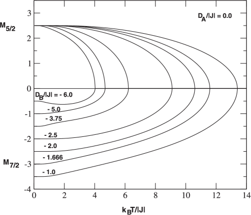
Figure 1: Thermal variation of the sublattice magnetizations $M_{5/2}$ and $M_{7/2}$ for the Blume-Capel model defined in the text, when the value of $D_{\text{B}}/|J|$ is varied for $D_{\text{A}}/|J|=0$.

Figure 2: Thermal variation of the sublattice magnetizations $M_{5/2}$ and $M_{7/2}$ for the mixed spin Blume-Capel model, when the value of $D_{\text{A}}/|J|$ is varied for $D_{\text{B}}/|J|=0$.

In figure 2, the effect of the crystal field $D_{\text{A}}/|J|$ is evaluated. Here, five saturation values are recovered for $M_{5/2}$ while $M_{7/2}$ shows a unique saturation value. These results look similar to those displayed in figure 1. Similar trends have been also reported in [30, 31].

Figure 3 illustrates, for $D_{\text{A}}/|J|=4$, the behaviour of the total magnetization per spin as a function of the temperature, for selected values of the reduced crystal field $D_{\text{B}}/|J|$. It turns out that compensation phenomena exist in the model where the global magnetization vanishes below the critical temperature. The strength of the crystal field affects both compensation and critical temperatures ($T_{\text{comp}}$ and $T_{\text{c}}$). An increase of the absolute value of this field leads to a decrease of $T_{\text{comp}}$. This behaviour also agrees with results from [34, 35].

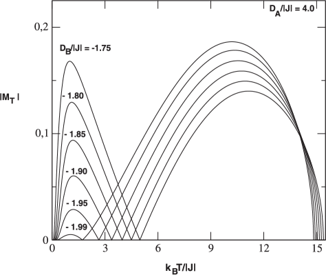
Figure 3: Behaviour of the total magnetization of the system $|M_{T}|$ as a function of the temperature for $D_{\text{A}}/|J|=4.0$ and negative values of $D_{\text{B}}/|J|$.

In figure 4, the thermal variations of sublattice and global magnetizations and the free energy of the system for $D_{\text{A}}/|J|=D_{\text{B}}/|J|=D/|J|-1.85$ are illustrated. An interesting trend is observed at low temperature: the existence of simultaneous jumps in four physical quantities. This is a strong proof of the existence of first-order transitions in the model for specific values of the model parameters. Such results are certainly the most exciting ones generated through the present study. The first-order transition temperature is indicated in figure 4 by $T_{\text{t}}$.

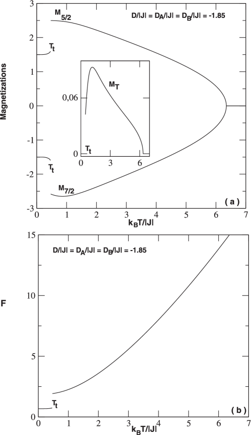
Figure 4: Temperature dependence of sublattice magnetizations, the total magnetization and the free energy for $D/|J|=D_{\text{A}}/|J|=D_{\text{B}}/|J|=-1.85$. From different panels, one can conclude that the model exhibits first-order transitions where jumps appear in different thermodynamical quantities presented. $T_{\text{t}}$ indicates the first-order temperature.

Figure 5 indicates the temperature-dependence of the global magnetization of the system. Obviously, six types of behaviours, namely Q-, R-, S-, N-, P- and L-types, are obtained according to their classification in the extended Néel nomenclature [36, 37, 38].

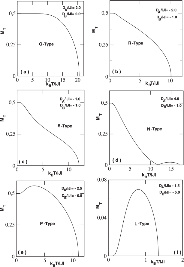
Figure 5: Temperature-dependence of the total magnetization $M_{T}$ for selected values of the crystal field. The model shows the Q-, R-, S-, N-, P- and L-types of compensation behaviours as classified in the extended Néel nomenclature.

The previous results on the thermal variations of the order parameters are useful in drawing the phase diagrams of the system. We present and illustrate these findings on the phase diagrams in the $(D_{\text{A}}/|J|,k_{\text{B}}T/|J|)$ plane for constant values of $D_{\text{B}}/|J|$ and on the $(D_{\text{B}}/|J|,k_{\text{B}}T/|J|)$ plane for constant values of $D_{\text{A}}/|J|$. The case of equal strengths of the reduced crystal fields, $D_{\text{A}}=D_{\text{B}}$ on the $(D/|J|,k_{\text{B}}T/|J|)$ plane was also investigated. In different phase diagrams constructed, the solid, dotted and dashed lines, respectively, denote second-order transition, first-order transition and compensation lines.

Through figure 6, it emerges that the critical temperature $T_{\text{c}}$, for not too large values of the sublattice crystal field decreases with decreasing values of the field strength. On the contrary, for relatively large values of the sublattice crystal field, it appears that the critical temperature becomes not sensitive to the strength of that field. Similar results have been reported in reference [39] where a new approach is used to generate the exact phase diagrams of the mixed spin-1/2 and spin-$S$ Ising model on a square lattice. Therein, the derived exact critical temperature tends to the exact value of the nearest neighbour spin-1/2 Ising model obtained by Onsager [40] as $D/J\rightarrow-\infty$. In figure 6 (a), for $D_{\text{A}}/|J|\rightarrow\infty$ $(-\infty)$ and $D_{\text{B}}/|J|\rightarrow-\infty$, the second-order transition temperature reaches a constant value at $12.93$ $(1.02)$ and for $D_{\text{B}}/|J|\rightarrow\infty$, this value of $k_{\text{B}}T_{\text{c}}/|J|$ is at $20.79$ $(5.43)$. Similarly, in figure 6 (c), as $D_{\text{B}}/|J|\rightarrow\infty$ $(-\infty)$ for $D_{\text{A}}/|J|\rightarrow-\infty$, the second-order transition temperature also reaches a constant value at $11.41$ $(1.02)$ and for $D_{\text{A}}/|J|\rightarrow\infty$, the constant value of $k_{\text{B}}T_{\text{c}}/|J|$ is at $25.91$ $(6.01)$. In figure 6 (b), values of $D_{\text{B}}/|J|$ are used to label transition lines. The second-order transition and compensation temperature lines are displayed from top to bottom for $D_{\text{B}}/|J|=-0.5,-0.75,-1.0,-1.5,-1.7$ and $-1.9$. In figure 6 (d), the roles of the sublattice crystal field were interchanged with respect to figure 6 (b). The figure illustrates lines of compensation temperature that merge at about $D_{\text{B}}/|J|=-2.0$ and terminate there.

Figure 6: While the phase diagrams on the $(D_{\text{A}}/|J|,k_{\text{B}}T/|J|)$ plane for constant values of $D_{\text{B}}/|J|$ are given in (a) and (b), the roles of the crystal field are illustrated in (c) and (d). (a) and (c) only present the second-order transition lines which are labeled with $D_{\text{B}}/|J|$ and $D_{\text{A}}/|J|$ values, respectively. (b) and (d) show the second-order transition lines and the lines of the compensation temperatures.

The constant value of $k_{\text{B}}T_{\text{c}}/|J|$ for negative values of $D$ originates from the fact that the lattice spins have the values $\pm 1/2$ in this region, the system being in the antiferromagnetic $(+1/2,-1/2)$ phase. The value $1.02$ found is about twice the value $0.56$ that we derived from MC calculations (not presented herein) on a system of size $N=100$ using $10^{5}$ MC steps per site. The MC result is of the order of the value $4k_{\text{B}}T_{\text{c}}/|J|=2.104$ found in reference [41] from an exact formulation of the spin-5/2 BC model. For large positive values of $D$, the system is in the phase $(5/2,-7/2)$ and the limiting value for the critical temperature is again about twice the value $11.3$ calculated in the above-mentioned reference.

In figure 7, we have depicted the phase diagram for the case of equal strengths of sublattice crystal fields. It turns out from the figure that when the value of the reduced crystal field $D/|J|\rightarrow\infty$ $(-\infty)$, the second-order phase transition temperature reaches the limiting values at about $25.22$ $(1.02)$. It is important to mention that figure 7 presents some resemblances with figure 10 of [42]. Moreover, the system exhibits a first-order transition at low temperature and negative values of the crystal field. The corresponding transition line ends at $D/|J|=-2.0$ and does not connect to the second-order line to generate a tricritical point. This line presents some resemblances with the first-order transition line illustrated in figure 1 of [43].

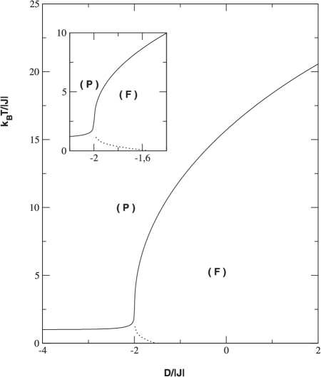
Figure 7: The phase diagram for equal values of the sublattice crystal fields $D/|J|=D_{\text{A}}/|J|=D_{\text{B}}/|J|$, in the $(D/|J|,k_{\text{B}}T/|J|)$ plane. The solid and dotted lines indicate the second- and first-order transition lines.

4 Conclusion

In this work, we examined the magnetic and critical properties of the mixed spin-$5/2$ and spin-$7/2$ Blume-Capel Ising system using the mean-field theory. The thermal variations of the order parameters have been shown. The behaviour of the global magnetization has been elucidated using the extended Néel classification nomenclature. Thus, Q-, R-, S-, N-, P- and L-types of compensation behaviours are got for appropriate values of the system parameters. Our results are in qualitative agreement with those computed by Monte Carlo simulations in reference [30]. In particular our figures 1; 2; 3 bear resemblances respectively with figures 6 and 7; 2 and 4; 9 of that reference. More interesting is the existence of the first-order transitions that we detected in the low temperature regime while analyzing the system behaviour for the case of equal crystal field strengths for both sublattices. Second-order phase transitions are also present with the existence of compensation points. Corresponding lines in the model parameters’ space have been presented.

Ukrainian 0 Ôàçîâi äiàãðàìè i êðèòèчíà ïîâåäiíêà çìiøàíî¿ ñïií-5/2 i ñïií-7/2 ñèñòåìè Içiíãà M. Êàðiìó${}^{\textsf{\footnotesize{\mbox{?},\penalty 1000\mbox{?}}}}$, Ð.À. Єññóôó${}^{\textsf{\footnotesize{\mbox{?},\penalty 1000\mbox{?}}}}$, Ã. Äiìiòði Íãàíöî${}^{\textsf{\footnotesize{\mbox{?}}}}$, Ô. Ãîíòiíôiíä${}^{\textsf{\footnotesize{\mbox{?},\penalty 1000\mbox{?}}}}$, E. Àëáàéðàê${}^{\textsf{\footnotesize{\mbox{?}}}}$

             
${}^{\textsf{\footnotesize 1}}$ Íàöiîíàëüíà âèùà øêîëà åíåðãåòèêè òà ïðîöåñiâ íàóêè (ENSGEP), óíiâåðñèòåò ì. Àáîìåé,
Ðåñïóáëiêà Áåíií ${}^{\textsf{\footnotesize 2}}$ Iíñòèòóò ìàòåìàòèêè i ôiçèчíèõ íàóê (IMSP), Ðåñïóáëiêà Áåíií ${}^{\textsf{\footnotesize 3}}$ Óíiâåðñèòåò ì. Àáîìåé-Êàëàâi, ôiçèчíèé âiääië, Ðåñïóáëiêà Áåíií ${}^{\textsf{\footnotesize 4}}$ GSMC, ôàêóëüòåò ïðèðîäíèчèõ íàóê i òåõíîëîãié, óíiâåðñèòåò Ìàðiàíà Íãóàái, Áðàççàâiëü, Êîíãî i LMPHE, ôàêóëüòåò ïðèðîäíèчèõ íàóê, óíiâåðñèòåò V Ìîõàììåäà, Ðàáàò, Ìîðîêêî ${}^{\textsf{\footnotesize 5}}$ Óíiâåðñèòåò Åðäæiєñ, ôiçèчíèé âiääië, 38039, Êàéñåði, Òóðåччèíà

References

- [1] Blume M., Phys. Rev., 1966, , 517, doi:10.1103/PhysRev.141.517.
- [2] Capel H.W., Physica, 1966, , 966, doi:10.1016/0031-8914(66)90027-9.
- [3] Lawrie I.D., Sarback S., In: Phase Transitions and Critical Phenomena, Vol. 9, Domb C., Lebowitz J.L. (Eds.), Academic Press, London, 1988, 2.
- [4] Siqueira A.F., Fittipaldi I.P., Phys. Rev. B, 1985, , 6092, doi:10.1103/PhysRevB.31.6092.
- [5] Siqueira A.F., Fittipaldi I.P., Physica A, 1986, , 592, doi:10.1016/0378-4371(86)90035-X.
- [6] Chakraborty K.G., Phys. Rev. B, 1984, , 1454, doi:10.1103/PhysRevB.29.1454.
- [7] Kaneyoshi T., J. Phys. C: Solid State Phys., 1988, , L679, doi:10.1088/0022-3719/21/18/004.
- [8] Kaneyoshi T., Physica A, 1992, , 436, doi:10.1016/0378-4371(92)90353-R.
- [9] Tucker J.W., J. Phys. C: Solid State Phys., 1988, , 6215, doi:10.1088/0022-3719/21/36/021.
- [10] Tucker J.W., J. Magn. Magn. Mater., 1987, , 27, doi:10.1016/0304-8853(87)90330-1.
-
[11]
Costabile E., Amazonas M.A., Viana J.R., de Sousa J.R., Phys. Lett. A, 2012, , 2922,
doi:10.1016/j.physleta.2012.09.003. - [12] Svendsen H., Overgaard J., Chevallier M.A., Collet E., Chen Y., Jensen F., Iversen B.B., Chemistry, 2010, , 7215, doi:10.1002/chem.200902997.
- [13] Özkan A., Phase Transitions, 2016, , 94, doi:10.1080/01411594.2015.1067702.
- [14] Karimou M., Yessoufou R.A., Ngantso G.D., Hontinfinde F., Benyoussef A., J. Supercond. Novel Magn., 2019, 32, 1769, doi:10.1007/s10948-018-4876-4.
- [15] Mallah T., Thiébaut S., Verdaguer M., Veillet P., Science, 1993, , 1554, doi:10.1126/science.262.5139.1554.
-
[16]
Manriquez J.M., Yee G.T., Mclean R.S., Epstein A.J., Miller J.S., Science, 1991, , 1415,
doi:10.1126/science.252.5011.1415. - [17] Jiang W., Wei G.Z., Zhang Z.D., Phys. Rev. B, 2003, , 134432, doi:10.1103/PhysRevB.68.134432.
- [18] Binasch G., Grünberg P., Saurenbach F., Zinn W., Phys. Rev. B, 1989, , 4828, doi:10.1103/PhysRevB.39.4828.
-
[19]
Sayama J., Asahi T., Mizutani K., Osaka T., J. Phys. D: Appl. Phys., 2004, , L1,
doi:10.1088/0022-3727/37/1/L01. - [20] Kaneyoshi T., Chen J.C., J. Magn. Magn. Mater., 1991, , 201, doi:10.1016/0304-8853(91)90444-F.
-
[21]
Wang C.L., Xin Y., Wang X.S., Zhong W.L., Zhang P.L., Phys. Lett. A, 2000, , 117,
doi:10.1016/S0375-9601(00)00145-6. -
[22]
Wang W., Lv D., Zhang F., Bi J., Chen J., J. Magn. Magn. Mater., 2015, , 16,
doi:10.1016/j.jmmm.2015.02.070. - [23] Jabar A., Tahiri N., Bahmad L., Benyoussef A., Physica A, 2016, , 1067, doi:10.1016/j.physa.2016.06.137.
- [24] Deviren B., Canko O., Keskin M., J. Magn. Magn. Mater., 2008, , 2291, doi:10.1016/j.jmmm.2008.04.130.
-
[25]
Bouziane T., Belaaraj A., Phys. Status Solidi B, 1999, , 387,
doi:10.1002/(SICI)1521-3951(199908)214:2%3C387::AID-PSSB387%3E3.0.CO;2-Y. - [26] Albayrak E., Aker A., J. Magn. Magn. Mater., 2010, , 3281, doi:10.1016/j.jmmm.2010.06.009.
- [27] Eddahri S., Karimou M., Razouk A., Hontinfinde F., Benyoussef A., Condens. Matter Phys., 2018, , 13705, doi:10.5488/CMP.21.13705.
- [28] Albayrak E., Yigit A., Phys. Status Solidi B, 2007, , 748, doi:10.1002/pssb.200642098.
- [29] Gonçalves L.L., Phys. Scr., 1985, , 248, doi:10.1088/0031-8949/32/3/012.
-
[30]
Bahlagui T., El Kenz A., Benyoussef A., J. Supercond. Novel Magn., 2018, 31, 4179,
doi:10.1007/s10948-018-4698-4. - [31] Bahlagui T., Bouda H., El Kenz A., Bahmad L., Benyoussef A., Superlattices Microstruct., 2017, 110, 90, doi:10.1016/j.spmi.2017.09.001.
- [32] Bogolubov N., J. Phys. USSR, 1947, 11, 23.
- [33] Feynman R.P., Phys. Rev., 1955, , 660, doi:10.1103/PhysRev.97.660.
- [34] Ekiz C., J. Magn. Magn. Mater., 2005, , 759, doi:10.1016/j.jmmm.2004.11.532.
- [35] De La Espriella Vélez N., Ortega López C., Torres Hoyos F., Rev. Mex. Fis., 2013, , 95.
- [36] Néel M.L., Ann. Phys., 1948, , 137, doi:10.1051/anphys/194812030137.
- [37] Strečka J., Physica A, 2006, , 379, doi:10.1016/j.physa.2005.07.012.
- [38] Yüksel Y., Aydıner E., Polat H., J. Magn. Magn Mater., 2011, , 3168, doi:10.1016/j.jmmm.2011.07.011.
- [39] Dakhama A., Azhari M., Benayad N., J. Phys. Commun., 2018, , 065011, doi:10.1088/2399-6528/aacbbe.
- [40] Onsager L., Phys. Rev., 1944, , 117, doi:10.1103/PhysRev.65.117.
- [41] Kaneyoshi T., Jaščur M., Phys. Status Solidi B, 1993, , 225, doi:10.1002/pssb.2221750119.
- [42] Karimou M., Yessoufou R.A., Oke T.D., Kpadonou A., Hontinfinde F., Condens. Matter Phys., 2016, , 33003, doi:10.5488/CMP.19.33003.
- [43] Albayrak E., Yigit A., Phys. Lett. A, 2006, , 121, doi:10.1016/j.physleta.2005.12.077.
Ukrainian \adddialect\l@ukrainian0 \l@ukrainian Ôàçîâi äiàãðàìè i êðèòèчíà ïîâåäiíêà çìiøàíî¿ ñïií-5/2 i ñïií-7/2 ñèñòåìè Içiíãà M. Êàðiìó, Ð.À. Єññóôó, Ã. Äiìiòði Íãàíöî, Ô. Ãîíòiíôiíä, E. Àëáàéðàê