Linking artificial and human neural representations of language

Abstract

What information from an act of sentence understanding is robustly represented in the human brain? We investigate this question by comparing sentence encoding models on a brain decoding task, where the sentence that an experimental participant has seen must be predicted from the fMRI signal evoked by the sentence. We take a pre-trained BERT architecture as a baseline sentence encoding model and fine-tune it on a variety of natural language understanding (NLU) tasks, asking which lead to improvements in brain-decoding performance.

We find that none of the sentence encoding tasks tested yield significant increases in brain decoding performance. Through further task ablations and representational analyses, we find that tasks which produce syntax-light representations yield significant improvements in brain decoding performance. Our results constrain the space of NLU models that could best account for human neural representations of language, but also suggest limits on the possibility of decoding fine-grained syntactic information from fMRI human neuroimaging.

What are the neural representations which support human language understanding? Language neuroscience has converged on a set of reliable physiological markers related to language processing (Kutas and Federmeier, 2011), and a picture of where in the brain different aspects of language processing take place (Fedorenko et al., 2010). But we still largely lack a coherent picture of the structure and format of the neural representations driving language understanding.

Part of this struggle is due to a scarcity of candidate representational structures in the first place. While there are certainly enough representational theories of language understanding, many are specified at too high a level of analysis to plausibly map onto neural structures without serious further revision (Poeppel, 2012).

Studies which draw on these high-level representations must therefore also assume some link between such representations and measures of neural activity — for example, that the magnitude of neural activations should match up with the probability values derived from a computational model (Brennan et al., 2016), or measures derived from syntactic representations of the input (Pallier et al., 2011). While the success of these mapping studies demonstrates that specific summary statistics of linguistic representations have correlates in the mind, these summary statistics are not themselves candidate representations for the fundamental operations underlying language understanding.

In the meantime, research in natural language processing has produced neural network models that capture many different sorts of intelligent language understanding behavior (Collobert et al., 2011; Goldberg, 2016). These models accomplish this behavior in an implementation better matched with that of the brain, with information about their inputs distributed across a high-dimensional continuous space. Could these models be taken seriously as candidate hypotheses of how language processing could be implemented in neural hardware? Under the assumption that both human brain and neural network representations are optimally suited to solve some task (Anderson et al., 1990), linking these two computational systems should reveal parallel task-optimal structure shared within their representations.

This paradigm linking brain and machine has already seen substantial success in vision science. Yamins et al. (2013) first demonstrated that the activations of a convolutional neural network trained on ImageNet in response to natural images could predict activations in a macaque monkey’s visual cortex in response to the same images. This result and others have led to an increasingly detailed understanding of the contents of brain representations (Schrimpf et al., 2018) and novel artificial neural network architectures (Kubilius et al., 2018) in the domain of vision.

In language understanding, several authors have exploited neural network representations as proxies for sentence meaning, and demonstrated that human brain activations in response to sentences can match with these meaning representations at well above chance performance (see e.g. Mitchell et al., 2008; Wehbe et al., 2014; Huth et al., 2016; Pereira et al., 2018). Our aim in this paper is to further understand why these mappings are successful, uncovering the parallel representational contents shared between human brains and neural networks.

We evaluate the link between human brain activity and neural network models as the models are optimized for different tasks. We find that neural network models quickly diverge in their capacity to match human brain activations as they are optimized for different NLU objectives. We further locate correlates of these changes in representational content, finding that the granularity of a model’s syntactic representations is at least partially responsible for their differences in brain decoding performance. Overall, this approach allows us to generate and validate hypotheses about the representational contents of both human brain and neural network activity.

1 Related work

Several papers have begun to explore the brain–machine link in language understanding, asking whether human brain activations can be matched with the activations of computational language models. Mitchell et al. (2008) first demonstrated that distributional word representations could be used to predict human brain activations, when subjects were presented with individual words in isolation. Huth et al. (2016) replicated and extended these results using distributed word representations, and Pereira et al. (2018) extended these results to sentence stimuli. Wehbe et al. (2014), Qian et al. (2016), Jain and Huth (2018), and Abnar et al. (2019) next introduced more complex word and sentence meaning representations, demonstrating that neural network language models could better account for brain activation by incorporating representations of longer-term linguistic context. Gauthier and Ivanova (2018) and Sun et al. (2019) further demonstrated that optimizing model representations for different objectives yielded substantial differences in brain decoding performance. This paper extends the neural network brain decoding paradigm both in breadth, studying a wide class of different task-optimal models, and in depth, exploring the particular representational contents of each model responsible for its brain decoding performance.

2 Methods

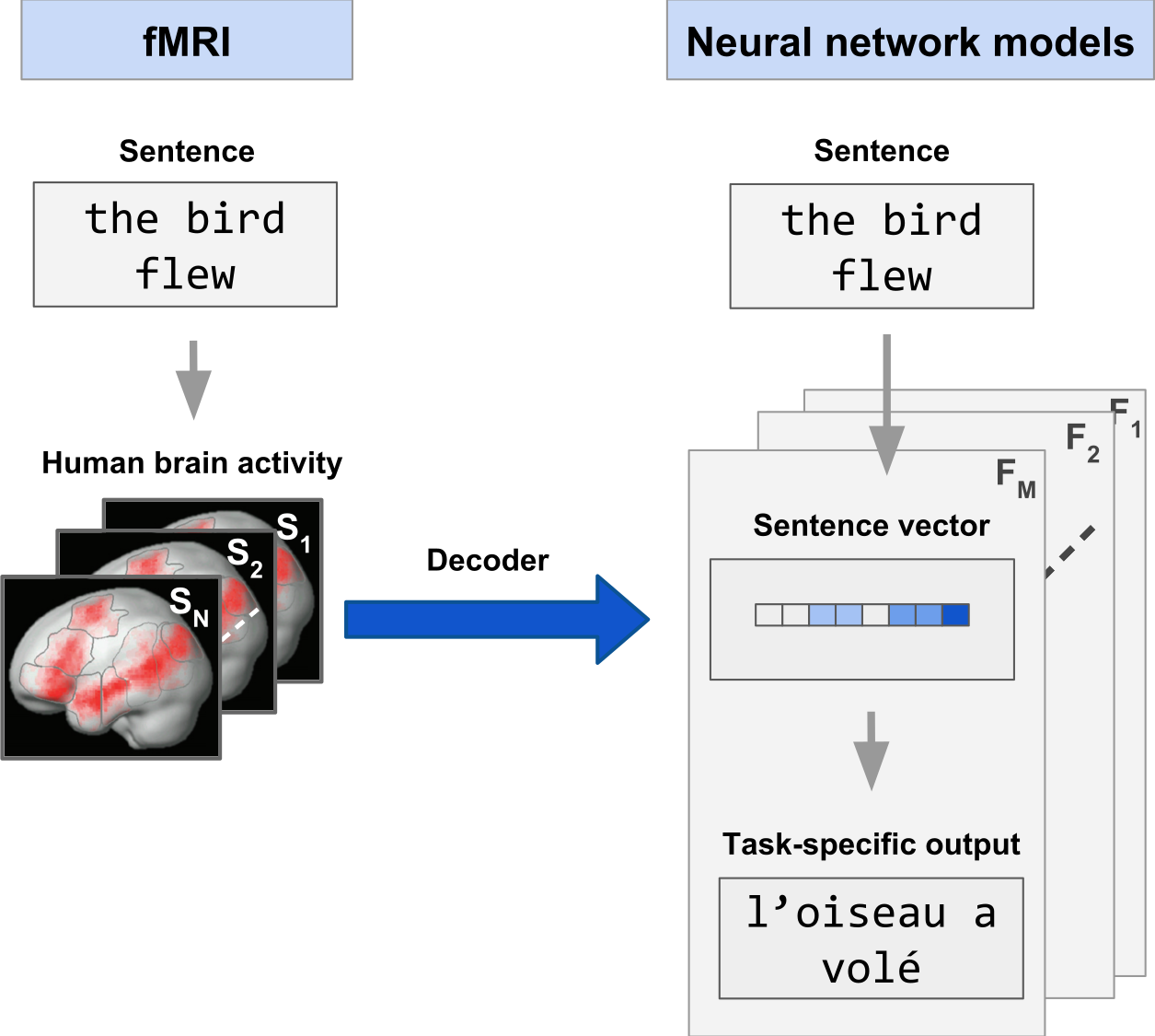
Figure 1: Brain decoding methodology. We use human brain activations in response to sentences to predict how neural networks represent those same sentences.

Figure 1 describes the high-level design of our experiments, which attempt to match human neuroimaging data with different candidate model representations of sentence inputs. Using a dataset of human brain activations recorded in response to complete sentences, we learn linear regression models which map from human brain activity to representations of the same sentences produced by different natural language understanding models.

To the extent that this linear decoding is successful, it can reveal parallel structure between brain and model representations. Consider a softmax neural network classifier model optimized for some task $T$, mapping input sentences $\mathbf{x}$ to class outputs $y$. We can factor this neural network classifier into the composition of two operations, a representational function $r(\mathbf{x})$, and an affine operator $A$:

$$p(y\mid\mathbf{x})\propto\exp({A(r(\mathbf{x}))})$$ (1)

Under this factorization, $r(\mathbf{x})$ must compute representations which are linearly separable with respect to the classes of the task $T$.

Research in cognitive neuroscience has shown that surprisingly many features of perceptual and cognitive states are likewise linearly separable from images of human brain activity, even at the coarse spatial and temporal resolution afforded by functional magnetic resonance imaging (fMRI; see e.g. Haxby et al., 2001; Kriegeskorte et al., 2006). However, the full power of linear decoding with fMRI remains unknown within language neuroscience and elsewhere. One possibility (1) is that the representational distinctions intrinsically required to describe language understanding behavior are linearly decodable from fMRI data. If this were the case, we could use performance in brain decoding to gauge the similarity between the mental representations underlying human language understanding and those deployed within artificial neural network models. Conversely (2), if the representations supporting language understanding in the brain are not linearly decodable from fMRI, we should be able to demonstrate this fact by showing specific ablations of sentence representation models do not degrade in brain decoding performance. Thus, the brain decoding framework offers possibilities both for (1) discriminating among NLU tasks as faithful characterizations of human language understanding, and for (2) understanding potential limitations of fMRI imaging and linear decoding methods. We explore both of these possibilities in this paper.

Section 2.1 describes the human neuroimaging data used as the source of this learned mapping. Section 2.2 next describes how we derive the target representations of sentence inputs from different natural language understanding models. Finally, Section 2.3 describes our method for deriving and evaluating mappings between the two representational spaces.

2.1 Human neuroimaging data

A man is a male human adult.

Fingers are used for grasping, writing, grooming and other activities.

Piranhas have very sharp teeth and are opportunistic carnivores.

Pressing a piano key causes a felt-tipped hammer to hit a vibrating steel string.

A range of mountains forms due to tectonic plate collision.

Table 1: Randomly sampled sentence stimuli from the human neuroimaging dataset of Pereira et al. (2018).

We use the human brain images collected by Pereira et al. (2018, experiment 2). Pereira et al. visually presented 384 natural-language sentences to 8 adult subjects. The sentences (examples in Table 1) consisted of simple encyclopedic statements about natural kinds, written by the authors. The subjects were instructed to carefully read each sentence, presented one at a time, and think about its meaning. As they read the sentences, the subjects’ brain activity was recorded with functional magnetic resonance imaging (fMRI). For each subject and each sentence, the fMRI images consist of a $\sim 200,000$-dimensional vector describing the approximate neural activity within small 3D patches of the brain, known as voxels. We collect these vectors in a single matrix and compress them to $d_{B}=256$ dimensions using PCA, yielding a matrix $B_{i}\in\mathbb{R}^{384{}\times d_{B}}$ for each subject $i$.

2.2 Sentence representation models

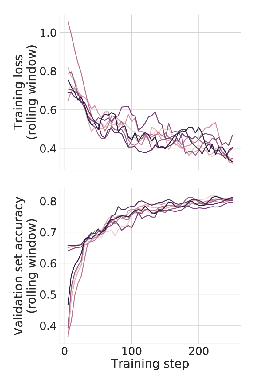
(a) QQP

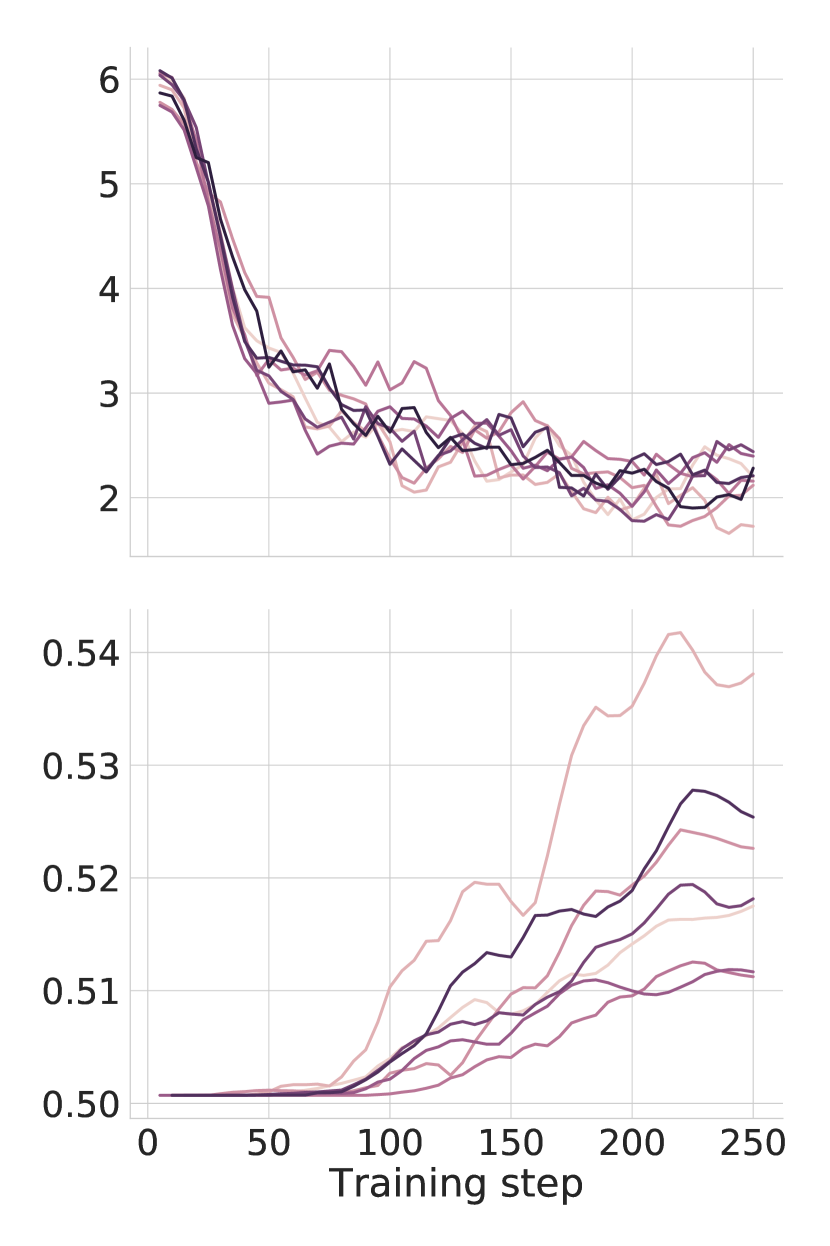
(b) SQuAD

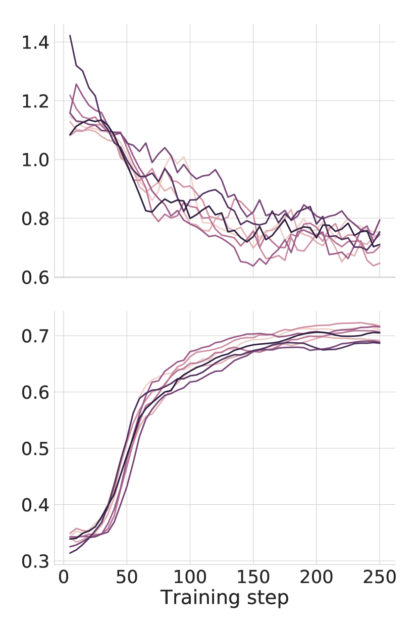
(c) MNLI

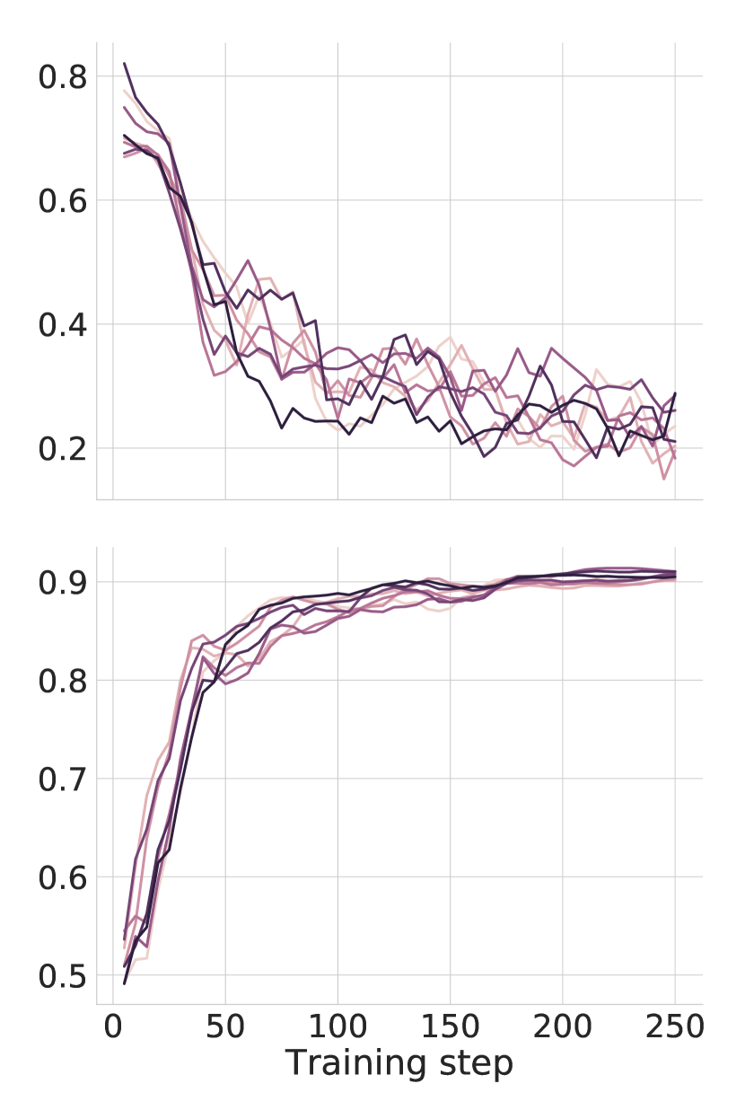
(d) SST

Figure 2: Learning curves (training set loss and evaluation set accuracy) for NLU model fine-tuning.

Task	Dataset	Domain	# train	Avg sent len.	# types
Paraphrase classification	Quora Question Pairs	social QA	364k	22.1	103k
Question answering	SQuAD 2.0 (Rajpurkar et al., 2018)	wiki	130k	11.2	43.9k
Natural language inference	MNLI (Williams et al., 2017)	mixed	393k	16.8	83.3k
Sentiment analysis	SST-2 (Socher et al., 2013)	movie reviews	67.3k	9.41	14.8k

Table 2: Details of the tasks used for fine-tuning.

We will match the human brain activation data described above with a suite of different sentence representations. Our primary concern in this evaluation is to compare alternative tasks and the representational contents they demand, rather than comparing neural network architectures. For this reason, we draw sentence representations from a unified neural network architecture — the bidirectional Transformer model BERT (Devlin et al., 2018) — as we optimize it to perform different tasks.

The BERT model uses a series of multi-head attention operations to compute context-sensitive representations for each token in an input sentence. The model is pre-trained on two tasks: (1) a cloze language modeling task, where the model is given a complete sentence containing several masked words and asked to predict the identity of a particular masked word; and (2) a next-sentence prediction task, where the model is given two sentences and asked to predict whether the sentences are immediately adjacent in the original language modeling data. For our purposes, this pre-training process produces a set of BERT parameters ${\Theta_{\text{LM}}}$ jointly optimized for these two objectives, consisting of word embeddings and attention mechanism parameters.

For an input token sequence $w_{1},\ldots,w_{T}$, the output of the BERT model is a corresponding sequence of contextualized representations of each token. We derive a single sentence representation vector by prepending a constant token $w_{0}=\texttt{[CLS]}$, and extracting its corresponding output vector at the final layer, following Devlin et al. (2018).

We first extract sentence representations from the pre-trained model parameterized by ${\Theta_{\text{LM}}}$. We let $C_{\text{LM}}\in\mathbb{R}^{384\times d_{H}}$ refer to the matrix of sentence representations drawn from this pre-trained BERT model, where $d_{H}$ is the dimensionality of the BERT hidden layer representation.

2.2.1 Fine-tuned models

We use the code and pre-trained weights released by Devlin et al. (2018) to fine-tune the BERT model on a suite of natural language processing classification tasks, shown in Table 2. This fine-tuning process jointly optimizes the pre-trained word embeddings and attention weights drawn from ${\Theta_{\text{LM}}}$, along with a task-specific classification model which accepts the sentence representations produced by the BERT model (the vector corresponding to the prepended [CLS] token) as input.

We fine-tune the pretrained BERT model on a set of popular shared NLU tasks, shown in Table 2, with fixed hyperparameters across tasks (available in Appendix B). Each fine-tuning operation is run for 250 iterations, before which all models show substantial improvements on the fine-tuning task. Figure 2 shows the learning curves for each of the models fine-tuned by this procedure.

We execute 8 different runs for each fine-tuning task. Each run $\ell$ of each fine-tuning task $j$ produces a set of final parameters ${\Theta_{j\ell}}$. We can derive a set of sentence representations $C_{j\ell}$ from each fine-tuned model by the same logic as above, feeding in each sentence with a prepended [CLS] token and extracting the contextualized [CLS] representation.

For our purposes, the product of each fine-tuning run is a set of sentence representations $C_{j\ell}\in\mathbb{R}^{384\times d_{H}}$.

Custom tasks

In order to better understand why models might fail or succeed at brain decoding, we also produced several custom fine-tuning tasks. Each task was a modified form of the standard BERT cloze language modeling task, manipulated to strongly select for or against some particular aspect of linguistic representation.

Scrambled language modeling

We first design two language modeling tasks to select against fine-grained syntactic representation of inputs. We randomly shuffle words from the corpus samples used for language modeling, to remove all first-order cues to syntactic structure. Our first custom task, LM-scrambled, deals with sentence inputs where words are shuffled within sentences; our second task, LM-scrambled-para, uses inputs where words are shuffled within their containing paragraphs in the corpus.

By shuffling inputs in this way, we effectively turn the cloze task into a bag-of-words language modeling task: given a set of words from a sentence or a random draw of words from a paragraph, the model must predict a missing word. After optimizing models on these scrambled tasks, we design a probe to validate the effects of the task on the model’s syntactic representations. This probe is detailed in Section 3.2.2.

Part-of-speech language modeling

We next design a task, LM-pos, to select against fine-grained semantic representation of inputs. We do this by requiring a model to predict only the part of speech of a masked word, rather than the word itself. This manipulation removes pressure for the model to distinguish predictions between target words in the same syntactic class.

We repeat fine-tuning runs on each of these custom tasks 4 times per task, and see substantial improvements in held-out task performance for each of these custom tasks after just 250 steps of training. After fine-tuning, we extract sentence representation matrices $C_{j\ell}$ from each run $\ell$ of each these models.

Language modeling control

As a control, we also continue training on the original BERT language modeling objectives using text drawn from the Books Corpus (Zhu et al., 2015). We run 4 fine-tuning runs of this task, yielding representations $C_{\text{LM},\ell}$.

2.2.2 Word vector baseline

As a baseline comparison, we also include sentence representations computed from GloVe word vectors (Pennington et al., 2014). Unlike BERT’s word representations, these word vectors are insensitive to their surrounding sentential context. These word vectors have nevertheless successfully served as sentence meaning representations in prior studies (Pereira et al., 2018; Gauthier and Ivanova, 2018). We let $C_{\text{GloVe}}(w_{1},\ldots,w_{T})=\frac{1}{T}e(w_{t})$, where $e(w_{i})$ retrieves the GloVe embedding for word $w_{i}$.

2.3 Brain decoding

We next learn a suite of decoders: regression models mapping from descriptions of human brain activation to model activations in response to sentences. Let $B_{i}\in\mathbb{R}^{384\times d_{B}}$ represent the brain activations of subject $i$ in response to the 384 sentences in our evaluation set. For each subject and each sentence representation available (including both language model representations $C_{\text{LM}}$ and fine-tuned model representations $C_{j\ell}$), we learn a linear map $G_{i\to{}j\ell}:\mathbb{R}^{d_{H}\times d_{B}}$ between the two spaces which minimizes the regularized regression loss

$$J_{ij\ell}=||G_{i\to{}j\ell}B_{i}-C_{j\ell}||_{2}^{2}+\beta\,||G_{i\to{}j\ell}||_{2}^{2}$$ (2)

where $\beta$ is a regularization hyperparameter. For each subject’s collection of brain images and each target model representation, we train and evaluate the above regression model with nested 8-fold cross-validation (Cawley and Talbot, 2010). The regression models are evaluated under two metrics: mean squared error (MSE) in prediction of model activations, and average rank (AR):

$$\text{AR}(i,j,\ell)=\frac{1}{384}\sum_{k}\text{rank}((G_{i\to{}j\ell}B_{i})[k],C_{j\ell}[k])$$ (3)

where $\text{rank}((G_{i\to{}j\ell}B_{i})[k],C_{j\ell}[k])$ gives the rank of a ground-truth sentence representation $C_{j\ell}[k]$ in the list of nearest neighbors of a predicted sentence representation $(G_{i\to{}j\ell}B_{i})[k]$, ordered by increasing cosine distance.

These two metrics serve complementary roles: the MSE metric strictly evaluates the ability of human brain activations to exactly match the representational geometry of model activations, while the AR metric simply requires that the brain activations be able to support the relevant meaning contrasts between the 384 sentences tested.

3 Results

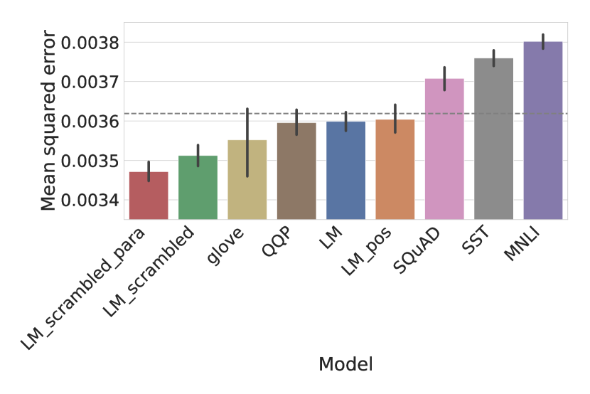
(a) Mean squared error metric

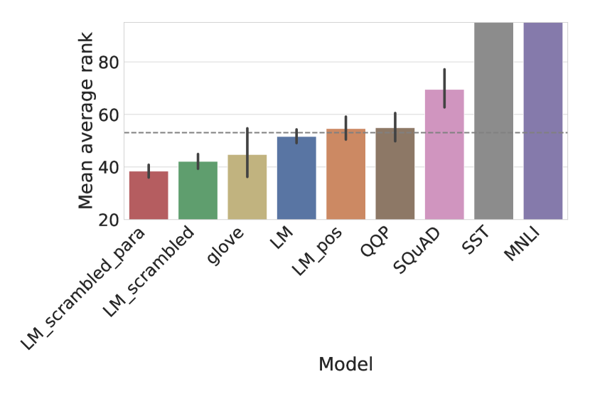
(b) Average rank metric

Figure 3: Brain decoding performance for fine-tuned BERT models and the GloVe baseline. Error bars are bootstrapped 95% confidence intervals, pooling across decoders matching different subjects (8 total) and different BERT fine-tuning runs (up to 8 runs per model). Dashed gray line shows the average brain decoding performance of the pretrained BERT language model.

We first present the performance of all of the BERT models tested and the GloVe baseline in Figure 3. This figure makes apparent a number of surprising findings, which we validate by paired $t$-tests.

1. On average, fine-tuning on the standard NLU tasks yields increased error in brain decoding under both metrics relative to the BERT baseline (MSE, $t\approx 14.8,p<3\times 10^{-36}$; AR, $t\approx 17,p<3\times 10^{-42}$). This trend is significant for each model individually, except QQP (MSE, $t\approx-2.2,p>0.03$; AR, $t\approx 0.79,p>0.4$).

2. Fine-tuning on the LM-scrambled-para custom task yields decreased error in brain decoding under both metrics relative to the BERT baseline (MSE, $t\approx-33.6,p<3\times 10^{-45}$; AR, $t\approx-26.9,p<5\times 10^{-39}$) and GloVe vectors (MSE, $t\approx-23.4,p<4\times 10^{-35}$; AR, $t\approx-12.1,p<6\times 10^{-19})$.

3. Fine-tuning on both the control language-modeling task and the LM-pos custom task yields ambiguous results: decreased MSE and no significant change in AR relative to the BERT baseline (LM-pos: MSE, $t\approx-2.90,p<0.007$; AR, $t\approx 2.10,p>0.04$; LM: MSE, $t\approx-5.68,p<4\times 10^{-7}$; AR, $t\approx-2.36,p>0.02$).

3.1 Learning dynamics

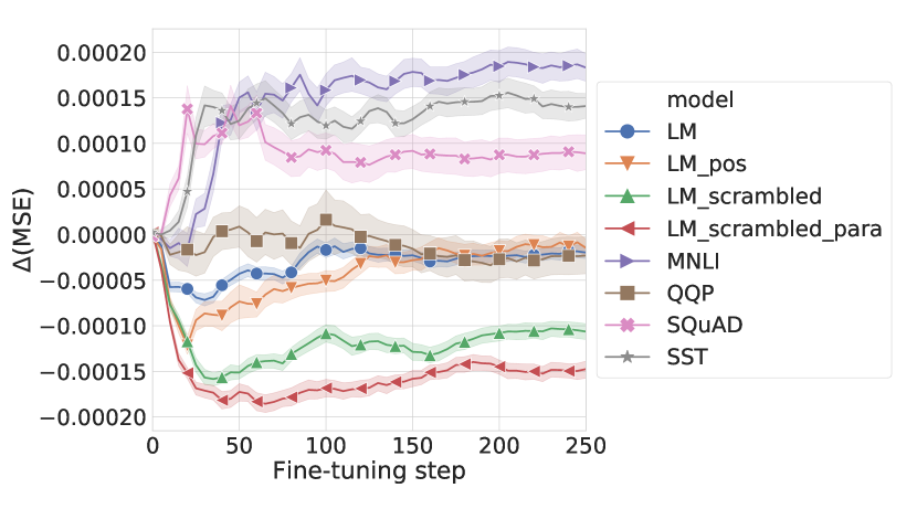
(a) Mean squared-error metric

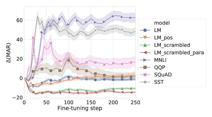
(b) Average rank metric

Figure 4: Brain decoding performance trajectories over fine-tuning time, graphed relative to the brain decoding performance of the pre-trained BERT language model. Performance rapidly diverges and then stabilizes within tens of fine-tuning steps. Shaded regions represent 95% confidence intervals, pooling across 8 subjects and up to 8 fine-tuning runs per model.

When during training do these models diverge in brain decoding performance? We repeat our brain decoding evaluation on model snapshots taken every 5 steps during fine-tuning, and chart brain decoding performance over time for each model in Figure 4. We find that models rapidly diverge in brain decoding performance, but remain mostly stable after about 100 fine-tuning steps. This phase of rapid change in brain decoding performance is generally matched with a phase of rapid change in task performance (compare each line in Figure 4 with the learning curves in Figure 2).

3.2 Representational analysis

We next investigate the structure of the model representations, and find that differing fidelity of syntactic representation can explain some major qualitative differences between the models in brain decoding performance.

3.2.1 Representational similarity

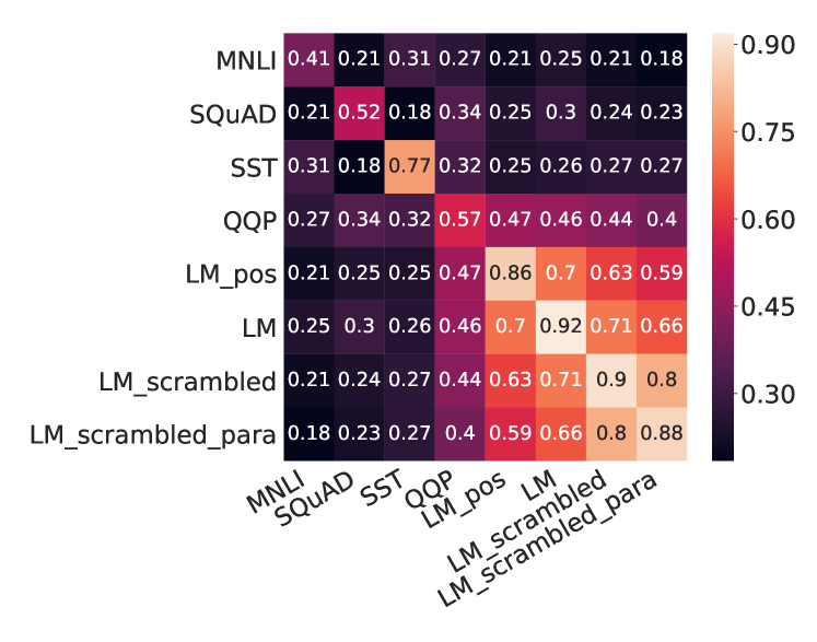
Figure 5: Representational similarity of the sentence encodings produced by each model (between -1 and 1; higher is more similar). See Section 3.2.1 for details.

We first investigate coarse-grained model similarity with representational similarity analysis (Kriegeskorte et al., 2008), which measures models’ pairwise distance judgments as a proxy for how well the underlying representations are aligned in their contents. For each fine-tuning run $\ell$ on each task $j$, we compute pairwise cosine similarities between each pair of sentence representation rows in $C_{j\ell}$, yielding a vector $D_{j\ell}\in\mathbb{R}^{(384{}\text{ choose }2)}$.

We measure the similarity between the representations derived from a run $(j,\ell)$ and some other run $(j^{\prime},\ell^{\prime})$ by computing the Spearman correlation coefficient $\rho(D_{j\ell},D_{j^{\prime}\ell^{\prime}})$. These correlation values are graphed as a heatmap in Figure 5, where each cell averages over different runs of the two corresponding models. This heatmap yields several clear findings:

1. The language modeling fine-tuning runs (especially the two LM-scrambled tasks) are the only models which have reliable high correlations between one another.

2. Language modeling tasks yield representations which make similar sentence-sentence distance predictions between different runs on the same task, while the rest of the models are less coherent across runs (see matrix diagonal).

The scrambled LM tasks produce sentence representations which are reliably coherent across runs (Figure 5), and produce reliable improvements in brain decoding performance (Figure 3). What is it about this task which yields such reliable results? We attempt to answer this question in the following section.

3.2.2 Syntactic probe

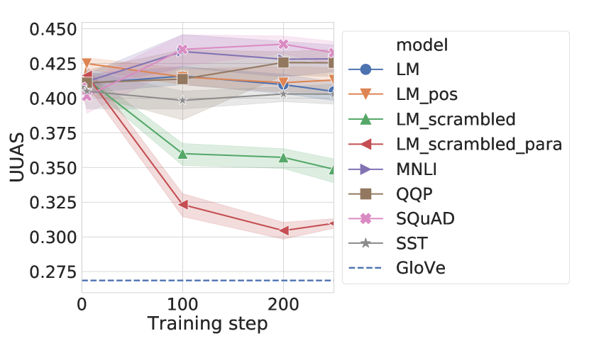
Figure 6: Syntactic probe evaluation across fine-tuning time (section 3.2.2).

Figure 7: Example sentence with undirected syntactic probe parses induced from LM-scrambled representations (blue, above) and GloVe representations (red, below). Solid arcs represent correct dependency predictions; dashed lines represent errors.

Because the scrambled LM tasks were designed to remove all first-order cues to syntactic constituency from the input, we hypothesized that the models trained on this task were succeeding due to their resulting coarse syntactic representations. We tested this idea using the structural probe method of Hewitt and Manning (2019). This method measures the degree to which word representations can reproduce syntactic analyses of sentences. We used dependency-parsed sentences from the Universal Dependencies (UD) English Web Treebank corpus (Silveira et al., 2014) to evaluate the performance of each fine-tuned BERT model with a structural probe.

For each fine-tuned BERT model (task $j$, fine-tuning run $\ell$) and each sentence $w_{1},\ldots,w_{T}$, let $\tilde{w_{i}}$ denote the context-sensitive representation of word $w_{i}$ under the model parameters ${\Theta_{j\ell}}$. The structural probe method attempts to derive a distance measure between context-sensitive word representations, parameterized by a transformation matrix $B$, which approximates the number of grammatical dependencies separating the two words (Hewitt and Manning, 2019). Concretely, for any two words $w_{i},w_{j}$ in a parsed sentence, we learn a parameter matrix $B$ such that

$$\left((B(\tilde{w_{i}}-\tilde{w_{j}}))^{T}(B(\tilde{w_{i}}-\tilde{w_{j}}))\right)^{2}\approx|w_{i}\leftrightarrow w_{j}|$$ (4)

where $|w_{i}\leftrightarrow w_{j}|$ denotes the number of edges separating $w_{i}$ and $w_{j}$ in a dependency parse of the sentence.

We learn this parameter matrix $B$ for a set of training sentences randomly sampled from the UD corpus, and then apply the distance measure above to model representations for a set of held-out test sentences. For any sentence $w_{1},\ldots,w_{T}$, the measure induces a $T\times T$ pairwise distance matrix, where each entry $(i,j)$ predicts the distance (in grammatical dependencies) between words $i$ and $j$. By applying a minimum spanning tree algorithm to this matrix, we derive an (undirected) parse tree for the sentence which best matches the predictions of the distance measure. We measure the accuracy of the reconstructed tree by calculating its unlabeled attachment score (UAS) relative to ground-truth parses from the UD corpus.

We apply the probe described above to every fine-tuning run of each model, and to baseline GloVe representations. We expected the GloVe representations to perform worst, since they cannot encode any context-sensitive features of input words. The probe results are graphed over fine-tuning time in Figure 6, relative to a probe induced from the GloVe representations (dashed blue line). This analysis shows that the models optimized for LM-scrambled and LM-scrambled-para — the models which improve in brain decoding performance — progressively worsen under this syntactic probe measure during fine-tuning. Their probe performance remains well above the performance of the GloVe baseline, however.

Figure 7 shows a representative sample sentence with parses induced from the syntactic probes of LM-scrambled (after 250 fine-tuning steps) and the GloVe baseline. While both parses make many mistaken attachments (dashed arcs), the parse induced from LM-scrambled (blue arcs) makes better guesses about local attachment decisions than the parse from GloVe (red arcs), which seems to simply link identical and thematically related words. This is the case even though LM-scrambled is never able to exploit information about the relative positions of words during its training. Overall, this suggests that much (but not all) of the syntactic information initially represented in the baseline BERT model is discarded during training on the scrambled language modeling tasks. Surprisingly, this loss of syntactic information seems to yield improved performance in brain decoding.

4 Discussion

The brain decoding paradigm presented in this paper has led us to a set of scrambled language modeling tasks which best match the structure of brain activations among the models tested. Optimizing for these scrambled LM tasks produces a rapid but stable divergence in representational contents, yielding improvements in brain decoding performance (Figures 3 and 4) and reliably coherent predictions in pairwise sentence similarity (Figure 5). These changes are matched with a clear loss of syntactic information (Figure 6), though some minimal information about local grammatical dependencies is decodable from the model’s context-sensitive word representations (Figure 7).

We do not take these results to indicate that human neural representations of language do not encode syntactic information. Rather, we see several possible explanations for these results:

Limitations of fMRI.

Functional magnetic resonance imaging — the brain imaging method used to collect the dataset studied in this paper — may be too temporally coarse to detect traces of the syntactic computations powering language understanding in the human brain.

This idea may conflict with several findings in the neuroscience of language. For example, Brennan et al. (2016) compared how language models with different granularities of syntactic representation map onto human brain activations during passive listening of English fiction. They derived word-level surprisal estimates from n-gram models (which have no explicit syntactic representation) and PCFG models (which explicitly represent syntactic constituency). In a stepwise regression analysis, they demonstrated that the surprisal estimates drawn from the PCFG model explain variance in fMRI measures of brain activation not already explained by estimates drawn from the n-gram model.

Pallier et al. (2011) examined a different hypothesis linking mental and neural representations of language. They presented subjects with strings of words which contain valid syntactic constituents of different lengths. They assumed that, since subjects will attempt to construct syntactic analyses of the word strings, the length of the possible syntactic constituents in any stimulus should have some correlate in subjects’ neural activations. They found a reliable relationship between the size of the available constituents in the input and region-specific brain activations as measured by fMRI.

Our results are compatible with the idea that specific syntactic features like those discussed above are still represented in the brain at the time scale of fMRI. Figures 6 and 7 demonstrate, in fact, that the LM-scrambled models still retain some syntactic information (or correlates thereof), in that they clearly outperform a baseline model in predicting the syntactic parses of sentences.

While these brain mapping studies have detected particular summary features of syntactic computation in the brain, these summary features do not constitute complete proposals of syntactic processing. In contrast, each of the models trained in this paper constitutes an independent candidate algorithmic description of sentence representation. These candidate descriptions can be probed (as in Section 3.2.2) to reveal exactly why brain decoding fails or succeeds in any case.

Our paradigm thus enables us to next ask: what specific syntactic features are responsible for the improved performance of the LM-scrambled models? By further probing the models and designing ablated datasets, we plan to narrow down the particular phenomena responsible for the findings presented here. These results should act as a source of finer-grained hypotheses about what sort of syntactic information is preserved at coarse temporal resolutions, and allow us to resolve the conflict between our results those of Pallier et al. (2011) and Brennan et al. (2016), among others.

Limitations of the linking hypothesis.

Our linear linking hypothesis (presented in Section 2.3) that representations of syntactic structure are encoded entirely in the linear geometry of both neural networks and human brains. It is likely that some syntactic information — among other features of the input — are conserved in the fMRI signal, but not readable by a linear decoder. Future work should investigate how more complex transforms linking brain and machine can reveal parallel structure between the two systems.

Limitations of the data.

The fMRI data used in this study (presented in Section 2.1) was collected as subjects read sentences and were asked to simply think about their meaning. This vague task specification may have led subjects to engage only superficially with the sentences. If this were the case, these shallow mental representations might present us with correspondingly shallow neural representations — just the sort of representations which might be optimal for the simple tasks such as LM-scrambled and LM-scrambled-para. Future work should integrate brain images derived from different behavioral tasks, and study which model–brain relationships are conserved across these behaviors. Such studies could illuminate the degree to which there are genuinely task-general language representations in the mind.

Our broader framework of analysis promises to reveal further insights about the parallel contents between artificial and human neural representations of language. In this spirit, we have released our complete analysis framework as open source code for the research community, available at http://bit.ly/nn-decoding.

Appendix A Supplemental figures

Figure 8(b) shows the change in brain decoding performance after fine-tuning grouped by subject, under both the mean squared error and rank metrics.

Figure 8: Within-subject changes in brain decoding performance for different models, relative to the subject’s brain decoding performance with the pre-trained BERT model. Error bars are 95% CIs pooling across decoders learned for different runs of each model (up to 8 per model).

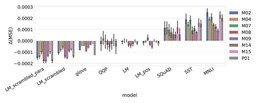
(a) Mean squared error metric

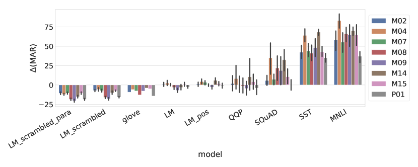
(b) Average rank metric

Figure 9(b) shows the change in brain decoding performance after fine-tuning grouped by model, under both the mean squared error and rank metrics.

Figure 9: Within-model changes in brain decoding performance for different subjects, relative to the corresponding subject’s brain decoding performance with the pre-trained BERT model. Error bars are 95% CIs pooling across decoders learned for different runs of each model (up to 8 per model).

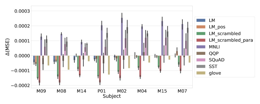
(a) Mean squared error metric

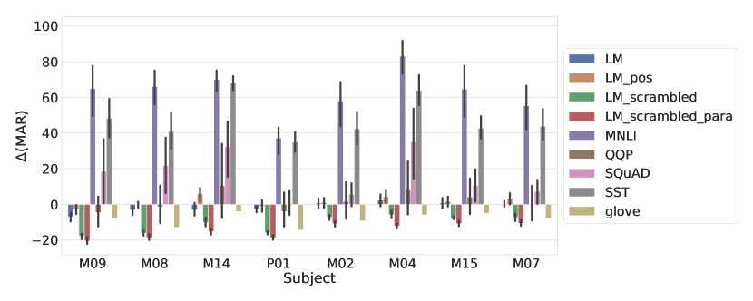
(b) Average rank metric

Appendix B Hyperparameters

Hyperparameter	Value
Batch size	32
Learning rate	$2\times 10^{-5}$
LR warmup proportion	10%
Maximum sequence length	128
Fine-tuning steps	250

Table 3: Fine-tuning hyperparameters, shared across fine-tuning runs for all tasks. These hyperparameters mostly follow the suggestions of Devlin et al. (2018).

Hyperparameter	Value
Training epochs	10
Loss metric	L1
Maximum rank of $B$	30
Positive semi-definite?	Yes

Table 4: Syntactic probe hyperparameters (Section 3.2.2), following the defaults of Hewitt and Manning (2019).

Appendix C Custom task information

For each language modeling task, we randomly sampled and concatenated documents from the Toronto Books Corpus (Kiros et al., 2015). Each language modeling dataset contained 1,000,000 training sentences and 100,000 development and test sentences. (We generated over-sized datasets in order to ensure that multiple runs of the same model would be highly unlikely to see similar samples of training data.)

For the part-of-speech task, we tagged each sentence using spaCy (Honnibal and Montani, 2017) and followed the same random masking procedure as in the typical cloze language modeling task. spaCy assigned 49 unique part-of-speech tags to the sentences, yielding a 49-way classification task.

For all tasks, we retained the secondary BERT objective requiring the model to predict whether two sentences are adjacent or not in a source document. (This objective did not differ from the standard setup for the part-of-speech task; for the scrambling task, the input sentences were independently randomly shuffled.)

Table 5(d) shows training examples from each of these custom tasks. Figure 10 shows learning curves and validation accuracy curves for the models trained on each task.

Table 5: Examples from custom language modeling tasks.

Input	Ground-truth output
[MASK] minutes in she began to cry .	two
the door opened and lilith [MASK] in with worry on her face .	walked
she grabbed several pairs of jeans and some t - shirts [MASK] her closet	from

(a) LM

Input	Ground-truth output
, and [MASK] so drive can .	i
instead ##k kn documents pots important dish water be ##s greasy , [MASK] were of of and soon legal in dirty ##ick personal ##ks high to a bath and looking pan awaiting the i with ago pan lifestyle face many ##ils d , years .	piles
by connected will if you the ##tell we the that ##i [MASK] us lead ?	people
, and i so drive can . abraham want , i myself i [MASK] cars and whenever his , two , dad	have

(b) LM-scrambled

Input	Ground-truth output
scent sweat ta very [MASK] aroma ##ed caught , , a close a his . ##ana cabaret sand male skin she ##wny of up and ##al mu ##ting slick faint …	##wood
, no in ! themselves supper with eyes included his ‘ , [MASK] began . the the alone everyone cried enjoying standing …	triumph
, she told off out would wash followed “ asked her i with ” take . voice [MASK] …	stepped

(c) LM-scrambled-para

Input	Ground-truth output
you ’ ve probably just gotten yourself off schedule a few days [MASK] you’ve been so busy and stressed .	CD
a couple of lordlings [MASK] .	VBD
the blond boy , who at fourteen was [MASK] much taller than anderra … showed no signs of discomposure .	RB

(d) LM-pos

Figure 10: Learning curves (training set loss and evaluation set accuracy) for custom language modeling tasks.

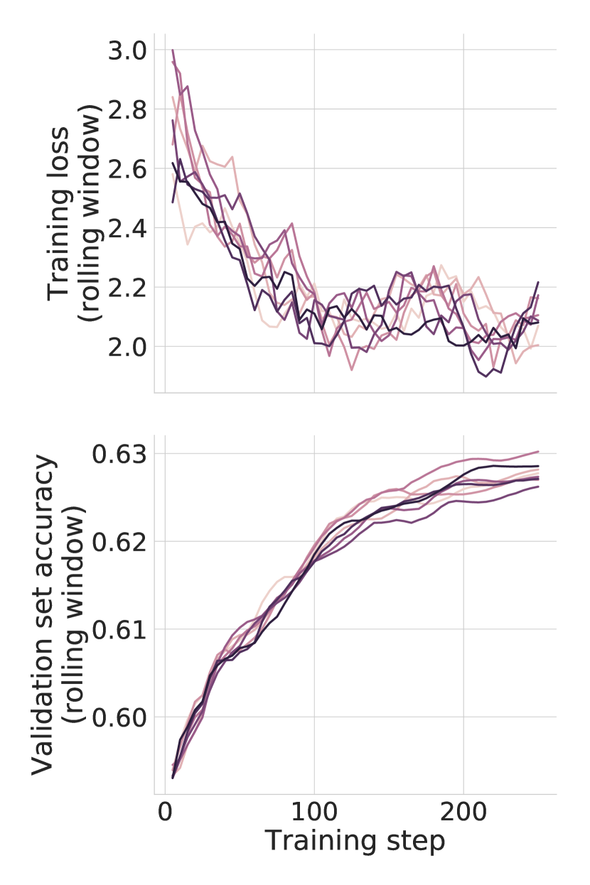
(a) LM (standard BERT task). Chance accuracy: $\frac{1}{30522}\approx 3\times 10^{-5}$.

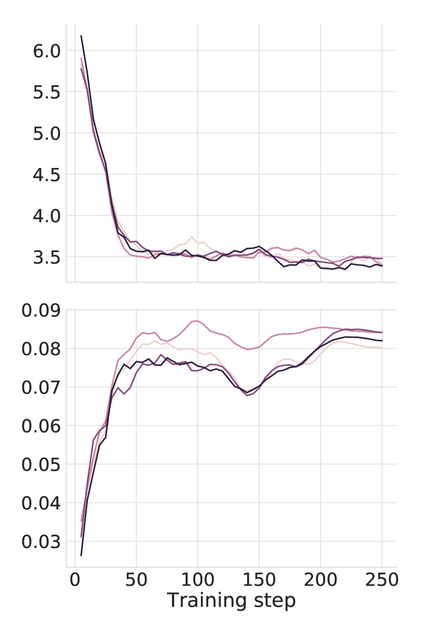
(b) LM-pos. Chance accuracy: $\frac{1}{49}\approx 0.02$.

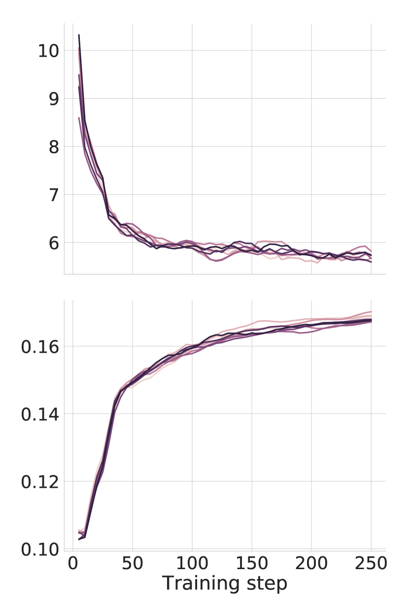
(c) LM-scrambled. Chance accuracy: $\frac{1}{30522}\approx 3\times 10^{-5}$.

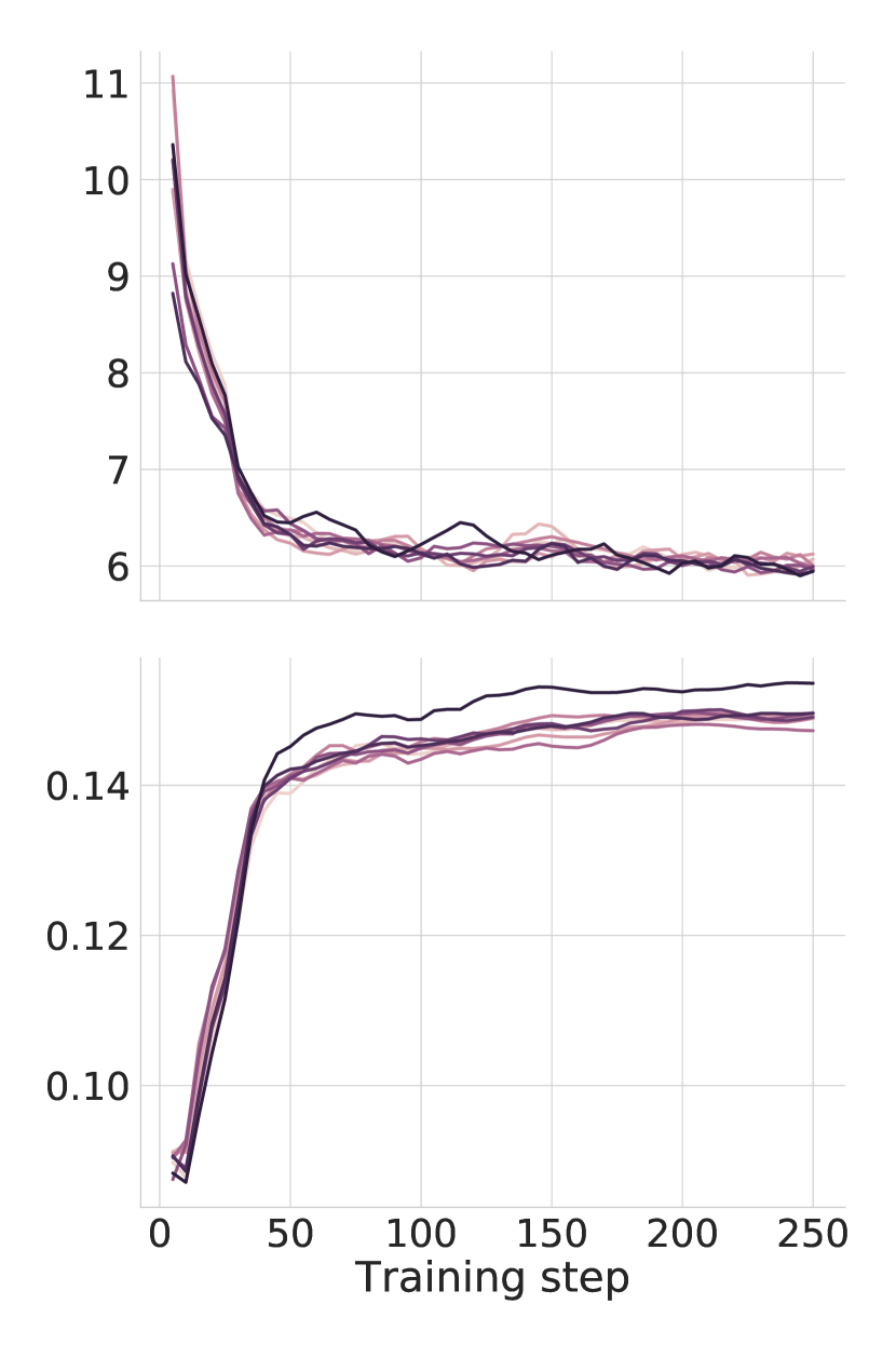
(d) LM-scrambled-para. Chance accuracy: $\frac{1}{30522}\approx 3\times 10^{-5}$.

References

- Abnar et al. (2019) Samira Abnar, Lisa Beinborn, Rochelle Choenni, and Willem Zuidema. 2019. Blackbox meets blackbox: Representational similarity and stability analysis of neural language models and brains. arXiv preprint arXiv:1906.01539.
- Anderson et al. (1990) John Robert Anderson et al. 1990. The Adaptive Character of Thought. Psychology Press.
- Brennan et al. (2016) Jonathan R Brennan, Edward P Stabler, Sarah E Van Wagenen, Wen-Ming Luh, and John T Hale. 2016. Abstract linguistic structure correlates with temporal activity during naturalistic comprehension. Brain and language, 157:81–94.
- Cawley and Talbot (2010) Gavin C Cawley and Nicola LC Talbot. 2010. On over-fitting in model selection and subsequent selection bias in performance evaluation. Journal of Machine Learning Research, 11(Jul):2079–2107.
- Collobert et al. (2011) Ronan Collobert, Jason Weston, Léon Bottou, Michael Karlen, Koray Kavukcuoglu, and Pavel Kuksa. 2011. Natural language processing (almost) from scratch. Journal of machine learning research, 12(Aug):2493–2537.
- Devlin et al. (2018) Jacob Devlin, Ming-Wei Chang, Kenton Lee, and Kristina Toutanova. 2018. Bert: Pre-training of deep bidirectional transformers for language understanding. arXiv preprint arXiv:1810.04805.
- Fedorenko et al. (2010) Evelina Fedorenko, Po-Jang Hsieh, Alfonso Nieto-Castañón, Susan Whitfield-Gabrieli, and Nancy Kanwisher. 2010. New method for fmri investigations of language: defining rois functionally in individual subjects. Journal of neurophysiology, 104(2):1177–1194.
- Gauthier and Ivanova (2018) Jon Gauthier and Anna Ivanova. 2018. Does the brain represent words? an evaluation of brain decoding studies of language understanding. In Proceedings of the 2nd Conference on Cognitive Computational Neuroscience, Philadelphia, Pennsylvania.
- Goldberg (2016) Yoav Goldberg. 2016. A primer on neural network models for natural language processing. Journal of Artificial Intelligence Research, 57:345–420.
- Haxby et al. (2001) James V Haxby, M Ida Gobbini, Maura L Furey, Alumit Ishai, Jennifer L Schouten, and Pietro Pietrini. 2001. Distributed and overlapping representations of faces and objects in ventral temporal cortex. Science, 293(5539):2425–2430.
- Hewitt and Manning (2019) John Hewitt and Christopher D Manning. 2019. A structural probe for finding syntax in word representations. In Proceedings of the 2019 Conference of the North American Chapter of the Association for Computational Linguistics: Human Language Technologies, NAACL-HLT, Minneapolis, Minnesota, USA, volume 2.
- Honnibal and Montani (2017) Matthew Honnibal and Ines Montani. 2017. spacy 2: Natural language understanding with bloom embeddings, convolutional neural networks and incremental parsing. To appear.
- Huth et al. (2016) Alexander G Huth, Wendy A de Heer, Thomas L Griffiths, Frédéric E Theunissen, and Jack L Gallant. 2016. Natural speech reveals the semantic maps that tile human cerebral cortex. Nature, 532(7600):453.
- Jain and Huth (2018) Shailee Jain and Alexander Huth. 2018. Incorporating context into language encoding models for fMRI. bioRxiv, page 327601.
- Kiros et al. (2015) Ryan Kiros, Yukun Zhu, Ruslan R Salakhutdinov, Richard Zemel, Raquel Urtasun, Antonio Torralba, and Sanja Fidler. 2015. Skip-thought vectors. In Advances in neural information processing systems, pages 3294–3302.
- Kriegeskorte et al. (2006) Nikolaus Kriegeskorte, Rainer Goebel, and Peter Bandettini. 2006. Information-based functional brain mapping. Proceedings of the National Academy of Sciences, 103(10):3863–3868.
- Kriegeskorte et al. (2008) Nikolaus Kriegeskorte, Marieke Mur, and Peter A Bandettini. 2008. Representational similarity analysis-connecting the branches of systems neuroscience. Frontiers in systems neuroscience, 2:4.
- Kubilius et al. (2018) Jonas Kubilius, Martin Schrimpf, Aran Nayebi, Daniel Bear, Daniel LK Yamins, and James J DiCarlo. 2018. Cornet: Modeling the neural mechanisms of core object recognition. BioRxiv, page 408385.
- Kutas and Federmeier (2011) Marta Kutas and Kara D Federmeier. 2011. Thirty years and counting: finding meaning in the n400 component of the event-related brain potential (erp). Annual review of psychology, 62:621–647.
- Mitchell et al. (2008) Tom M Mitchell, Svetlana V Shinkareva, Andrew Carlson, Kai-Min Chang, Vicente L Malave, Robert A Mason, and Marcel Adam Just. 2008. Predicting human brain activity associated with the meanings of nouns. Science, 320(5880):1191–1195.
- Pallier et al. (2011) Christophe Pallier, Anne-Dominique Devauchelle, and Stanislas Dehaene. 2011. Cortical representation of the constituent structure of sentences. Proceedings of the National Academy of Sciences, 108(6):2522–2527.
- Pennington et al. (2014) Jeffrey Pennington, Richard Socher, and Christopher Manning. 2014. Glove: Global vectors for word representation. In EMNLP.
- Pereira et al. (2018) Francisco Pereira, Bin Lou, Brianna Pritchett, Samuel Ritter, Samuel J Gershman, Nancy Kanwisher, Matthew Botvinick, and Evelina Fedorenko. 2018. Toward a universal decoder of linguistic meaning from brain activation. Nature communications, 9(1):963.
- Poeppel (2012) David Poeppel. 2012. The maps problem and the mapping problem: two challenges for a cognitive neuroscience of speech and language. Cognitive neuropsychology, 29(1-2):34–55.
- Qian et al. (2016) Peng Qian, Xipeng Qiu, and Xuanjing Huang. 2016. Bridging lstm architecture and the neural dynamics during reading. In Proceedings of the Twenty-Fifth International Joint Conference on Artificial Intelligence, pages 1953–1959. AAAI Press.
- Rajpurkar et al. (2018) Pranav Rajpurkar, Robin Jia, and Percy Liang. 2018. Know what you don’t know: Unanswerable questions for squad. arXiv preprint arXiv:1806.03822.
- Schrimpf et al. (2018) Martin Schrimpf, Jonas Kubilius, Ha Hong, Najib J Majaj, Rishi Rajalingham, Elias B Issa, Kohitij Kar, Pouya Bashivan, Jonathan Prescott-Roy, Kailyn Schmidt, et al. 2018. Brain-score: which artificial neural network for object recognition is most brain-like? BioRxiv, page 407007.
- Silveira et al. (2014) Natalia Silveira, Timothy Dozat, Marie-Catherine de Marneffe, Samuel Bowman, Miriam Connor, John Bauer, and Christopher D. Manning. 2014. A gold standard dependency corpus for English. In Proceedings of the Ninth International Conference on Language Resources and Evaluation (LREC-2014).
- Socher et al. (2013) Richard Socher, Alex Perelygin, Jean Wu, Jason Chuang, Christopher D Manning, Andrew Ng, and Christopher Potts. 2013. Recursive deep models for semantic compositionality over a sentiment treebank. In Proceedings of the 2013 conference on empirical methods in natural language processing, pages 1631–1642.
- Sun et al. (2019) Jingyuan Sun, Shaonan Wang, Jiajun Zhang, Chengqing Zong, et al. 2019. Towards sentence-level brain decoding with distributed representations. In Proceedings of the 33rd AAAI Conference on Artificial Intelligence (AAAI-2019).
- Vaswani et al. (2017) Ashish Vaswani, Noam Shazeer, Niki Parmar, Jakob Uszkoreit, Llion Jones, Aidan N Gomez, Łukasz Kaiser, and Illia Polosukhin. 2017. Attention is all you need. In Advances in Neural Information Processing Systems, pages 5998–6008.
- Wehbe et al. (2014) Leila Wehbe, Ashish Vaswani, Kevin Knight, and Tom Mitchell. 2014. Aligning context-based statistical models of language with brain activity during reading. In Proceedings of the 2014 Conference on Empirical Methods in Natural Language Processing (EMNLP), pages 233–243.
- Williams et al. (2017) Adina Williams, Nikita Nangia, and Samuel R Bowman. 2017. A broad-coverage challenge corpus for sentence understanding through inference. arXiv preprint arXiv:1704.05426.
- Yamins et al. (2013) Daniel L Yamins, Ha Hong, Charles Cadieu, and James J DiCarlo. 2013. Hierarchical modular optimization of convolutional networks achieves representations similar to macaque it and human ventral stream. In C. J. C. Burges, L. Bottou, M. Welling, Z. Ghahramani, and K. Q. Weinberger, editors, Advances in Neural Information Processing Systems 26, pages 3093–3101. Curran Associates, Inc.
- Zhu et al. (2015) Yukun Zhu, Ryan Kiros, Rich Zemel, Ruslan Salakhutdinov, Raquel Urtasun, Antonio Torralba, and Sanja Fidler. 2015. Aligning books and movies: Towards story-like visual explanations by watching movies and reading books. In The IEEE International Conference on Computer Vision (ICCV).