Rogue Waves and Periodic Solutions of a Nonlocal Nonlinear Schrödinger Model

Abstract

In the present work, a nonlocal nonlinear Schrödinger (NLS) model is studied by means of a recent technique that identifies solutions of partial differential equations, by considering them as fixed points in space-time. This methodology allows to perform a continuation of well-known solutions of the local NLS model to the nonlocal case. Four different examples of this type are presented, namely (a) the rogue wave in the form of the Peregrine soliton, (b) the generalization thereof in the form of the Kuznetsov-Ma breather, as well as two spatio-temporally periodic solutions in the form of elliptic functions. Importantly, all four waveforms can be continued in intervals of the parameter controlling the nonlocality of the model. The first two can be continued in a narrower interval, while the periodic ones can be extended to arbitrary nonlocalities and, in fact, present an intriguing bifurcation whereby they merge with (only) spatially periodic structures. The results suggest the generic relevance of rogue waves and related structures, as well as periodic solutions, in nonlocal NLS models.

I Introduction

The study of dispersive media exhibiting a nonlocal nonlinear response is a subject that is enjoying increasing attention over the past few years t28 ; assanto1 ; assanto2 . This is mainly due to the fact that relevant models and their solutions, especially of the nonlinear Schrödinger (NLS) variety, emerge in a wide range of physical contexts. These range from thermal optical media t28 ; t27 and nematic liquid crystals assanto1 ; assanto2 ; t25 and from plasmas t29 ; t30 to water waves hf1 ; hf2 and dipolar Bose-Einsein condensates bec1 ; bec2 . It is, thus, naturally of interest to explore the different types of solitary wave solutions that may arise in nonlocal NLS systems and how nonlocality may alter the properties and behavior of media with a local nonlinear response neshev ; krol2 ; krol3 .

Another topic of wide interest during the past decade has been the study of rogue (freak) waves, i.e., coherent structures of large amplitude that appear out of nowhere and disappear without a trace wandt . The study of such waves has been explored mainly in hydrodynamics hydro ; hydro2 ; hydro3 , but also in numerous other areas. These include, but are not limited to, nonlinear optics opt1 ; opt2 ; opt3 ; opt4 ; opt5 ; laser , superfluid helium He , as well as plasmas plasma . These multifaceted experimental studies have, in turn, triggered a wide range of theoretical explorations which by now have been summarized in a series of reviews onorato ; solli2 ; yan_rev ; Akhmediev2016 ; Chen2017 ; Mihalache2017 ; MalomedMihalache2019 , but also importantly in a series of books on this research theme k2a ; k2b ; k2c ; k2d .

In the present work, we combine these two cutting edge themes, by exploring rogue waves and related coherent structures in nonlocal media motivated by the above optical, liquid crystal and water wave applications. It should be noted that a search of the literature of rogue waves in nonlocal NLS models will yield a number of results, such as, e.g. jyang . However, these concern a mathematically motivated (via PT-symmetry and related considerations) nonlocal variant of the NLS AM . There is a paucity of results concerning rogue waves of physically relevant nonlocal NLS models, as e.g., the one considered in Ref. ha3 . However, this is rather understandable given the non-integrability of such models and the distinct lack of tools for tackling rogue waves beyond the integrable limit and its associated techniques, such as the inverse scattering method.

Here, we aim to provide a number of results regarding the model of the nonlocal NLS that is of wide relevance to applications. Our approach leverages a recently proposed technique reported in Ref. ward . In this work, it was recognized that it is difficult to identify rogue waves (contrary to what is the case with solitons), due to their non-stationary nature in time. However, considering them in space-time, i.e., treating time as a spatial direction, one realizes that rogue waves are localized solutions in that setting. Thus, one can —in principle— construct fixed point methods (based, e.g., on a conjugate gradient-based variant of the Newton method ward ) that will converge to such wave structures, and identify them as numerically exact solutions. A key advantage of such a methodology is that it does not hinge in any critical way on integrability and, indeed, starting from the integrable limit it can be used in a variety of non-integrable settings, such as the nonlocal one that we consider here. It is this tool that will permit us to converge to the rogue wave (in the form of the Peregrine soliton) for a range of parameter values of the nonlocality parameter, referred to as $\nu$ below in our model. In addition to the prototypical Peregrine structure, we will also seek its periodic —in the propagation variable— generalization, namely the Kuznetsov-Ma (KM) breather. Both of these will be found to be possible to continue within a certain interval of the nonlocality parameter (roughly up to $\nu=0.2$). Apart from these structures, we will also consider and identify additional states that our analysis can reveal in the nonlocal system, namely periodic states in space-time (starting from the elliptic function local limit). We will see that these can be continued for essentially arbitrary $\nu$, yet they feature a bifurcation becoming stationary (or independent of the propagation direction) beyond a certain critical threshold.

Our presentation will be structured as follows. In section II, we will present the solutions of interest in the local limit of the regular NLS model (i.e., for $\nu=0$). In section III, we will present the numerical extensions of the solutions via the above method to the nonlocal case of finite $\nu$. Finally, in section IV, we will summarize our findings and present our conclusions.

II The Model and Its Local Limit Solutions

We consider a nonlocal variant of the NLS model, which, in dimensionless form, can be expressed as ha3 ; assanto1 ; assanto2 :

$$i\frac{\partial u}{\partial t}+\frac{1}{2}\frac{\partial^{2}u}{\partial x^{2}}+\theta u-\mu u=0,$$ (1)

$$\nu\frac{\partial^{2}\theta}{\partial x^{2}}-2q\theta=-2|u|^{2}.$$ (2)

where $u=u(x,t)$, $\theta=\theta(x,t)$, and, in the context of nematic liquid crystals, $t$ plays the role of the propagation coordinate. The dependent variable $u$ is the complex valued, slowly varying envelope of the optical (electric) field, and $\theta$ is the optically induced deviation of the director angle. The nonlocality parameter $\nu$ measures the strength of the response of the nematic in space, with a highly nonlocal response corresponding to $\nu$ large. Notice that in the nonlocal regime with $\nu$ large, the optically induced rotation $\theta$ is small. The parameter $q$ is related to the square of the applied static field which pre-tilts the nematic dielectric, while $\mu$ plays the role of the propagation constant. Obviously, inclusion of the term $\mu u$ in Eq. (1) (which is normally omitted) offers a constant background where certain types of solutions (such as the Peregrine soliton —see below) can exist, and is trivially removed via a constant phase transformation. Hereafter, we set $q=1$.

The system (1)-(2) can be considered as a single integro-differential equation provided Fourier transforms are utilized. This will not limit our set of solutions however for we will make only numerical use of the transform pair. As such a periodic domain is used to integrate the system in $x$ and nondecaying functions will not generate problems with the transform not converging. Thus, using the Fourier Transform we can rewrite Eq. (2) as

$$\theta=\mathcal{F}^{-1}\left[\frac{\mathcal{F}[2|u|^{2}]}{\nu k^{2}+2}\right].$$ (3)

Plugging this into Eq. (1) yields a nonlocal equation in $u$ alone and will be the equation with which we work in our numerical computations hereafter. Note that when $\nu=0$ we recover the standard NLS equation.

The four solutions that will be of interest hereafter are analytically available in the NLS limit. The first one is the famous Peregrine soliton H_Peregrine ; for $\mu=1$, this solution reads:

$$u(x,t)=1-\frac{2(1+4it)}{1+4x^{2}+4t^{2}}.$$ (4)

This structure has been the subject of numerous recent experimental observations in hydrodynamics hydro , nonlinear optics opt2 , plasmas plasma , and so on.

The second one is the periodic generalization of the Peregrine soliton in the evolution direction, namely the so-called Kuznetsov-Ma (KM) breather given by kuz ; ma :

$$u(x,t)=1-\frac{2(b^{2}-1)\cos(2b\sqrt{b^{2}-1}t)+i2b\sqrt{b^{2}-1}\sin(2b\sqrt{b^{2}-1}t)}{b\cosh(2\sqrt{b^{2}-1}x)-\cos(2b\sqrt{b^{2}-1}t)},$$ (5)

where $b$ is an arbitrary parameter (with $b>1$). It is worthwhile to note that this solution has been experimentally observed as well opt3 .

We now consider some spatio-temporally periodic solutions stemming from the classic work of akh , both of them for simplicity given for $\mu=1/2$. The first is a doubly periodic solution given by:

$$u(x,t) = \frac{\kappa}{2}\;\frac{A(x){\rm cn}(t/2)+i\sqrt{1+\kappa}\;{\rm sn}(t,\kappa)}{\sqrt{1+\kappa}-A(x){\rm dn}(t/2,\kappa)},$$ (6)

$$A(x) = {\rm cd}\bigg{(}\sqrt{\frac{1+\kappa}{2}}x,\sqrt{\frac{1-\kappa}{1+\kappa}}\bigg{)},$$ (7)

where $\kappa$ is an arbitrary parameter (with $0<\kappa<1$). The second is another doubly periodic solution given by:

$$u(x,t)=\frac{\sqrt{\frac{\kappa}{1+\kappa}}{\rm cn}\big{(}\frac{x}{\sqrt{\kappa}},\sqrt{\frac{1-\kappa}{2}}\big{)}{\rm dn}\big{(}\frac{t}{2\kappa},\kappa\big{)}+i\kappa\;{\rm sn}\big{(}\frac{t}{2\kappa},\kappa\big{)}}{\kappa\sqrt{2}\big{[}1-\sqrt{\frac{\kappa}{1+\kappa}}{\rm cn}\big{(}\frac{x}{\sqrt{\kappa}},\sqrt{\frac{1-\kappa}{2}}\big{)}{\rm cn}\big{(}\frac{t}{2\kappa},\kappa\big{)}\big{]}},$$ (8)

where $\kappa$ is again an arbitrary parameter (with $0<\kappa<1$).

III Continuation to the Nonlocal Case

III.1 Peregrine Soliton

(a) $\nu=0$

(b) $\nu=0.05$

(c) $\nu=0.15$

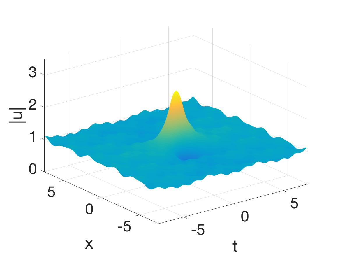
(d) $\nu=0.2$

Figure 1: Continuation over increasing $\nu$ values of the Peregrine rogue wave solution of the NLS. The absolute value of the wavefunction is shown as a function of space $x$ and time $t$, once the iterative identification of the solution converges.

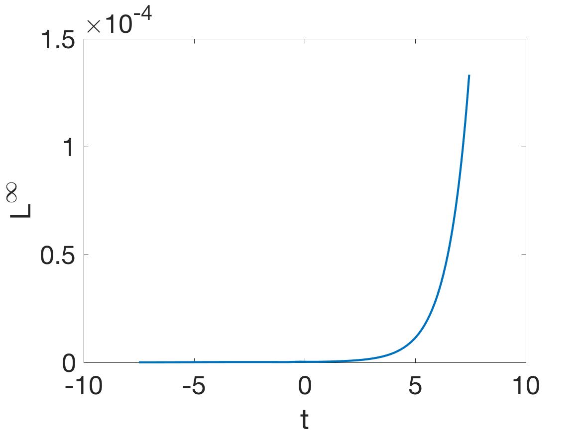
(a) $\nu=0$

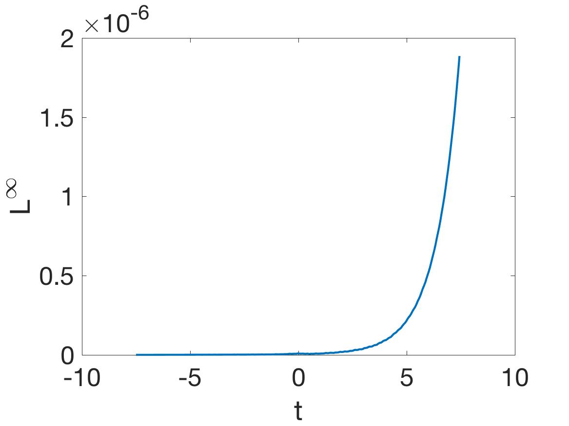
(b) $\nu=0.1$

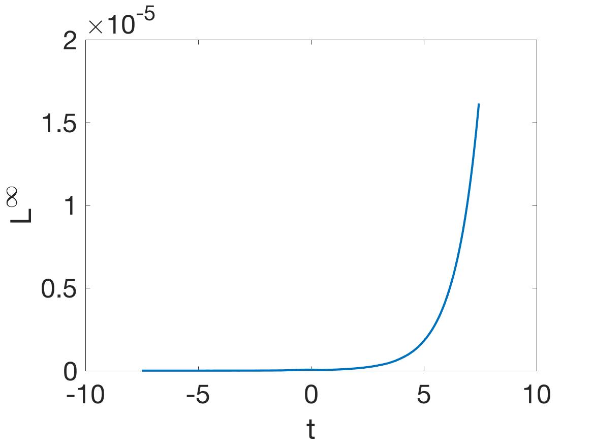
(c) $\nu=0.15$

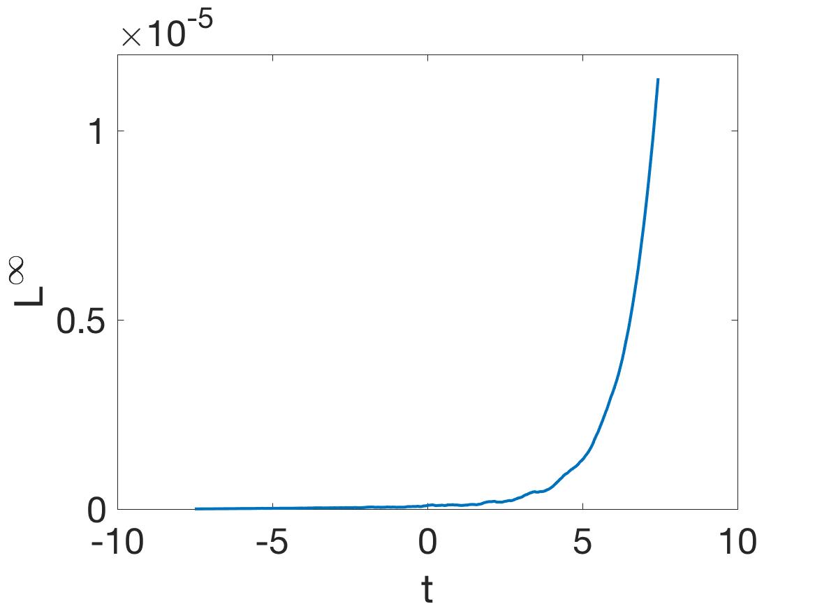
(d) $\nu=0.2$

Figure 2: $L^{\infty}$ error (i.e., norm of the difference) between the numerical ETDRK4 solution of Eqs. (1)-(2) and the converged Peregrine soliton waveform obtained by the Newton-CG method for the different case examples of nonlocality parameter $\nu$ shown in Fig. 1.

The results associated with the Peregrine soliton are given in Figs. 1 and 2. The first one, shows the profile of the Peregrine soliton as the value of the nonlocality parameter $\nu$ is increased. Perhaps the most important finding in itself is that this structure can still be obtained as a numerically exact solution beyond the integrable limit, and in the nonlocal case of $\nu\neq 0$. Structurally, it can be observed that the solution acquires a certain “undulation”, as $\nu$ is increased, that becomes progressively more pronounced. It is important to also highlight here that the solution is identified with periodic boundary conditions in both space and time (recall that time is treated as a space variable so a periodicity is imposed on that as well). The continuation scheme is unable to go past $\nu=0.2$, even when considering different domain sizes. Nevertheless, we do not detect a bifurcation at this point, hence it is unclear whether this is a trait of the solution or a by-product of the particular numerical method. We believe that the latter is true.

Figure 2, in turn, is a dynamical illustration of the accuracy of convergence of our solution. Here, what is done is that we select the “initial condition” of our converged Peregrine waveform at $t=-7.5$ and feed it into an integrator of the full nonlocal problem at different values of $\nu$. The forward propagation of Eqs. (1)-(2) is performed using the exponential time-differencing 4th-order Runge-Kutta (ETDRK4) method of Ref. Kassam . In the figure it is observed that the measured $L^{\infty}$ error (i.e., norm of the difference) between the converged solution and the numerically propagated one remains very small (i.e., of O$(10^{-4})$ to O$(10^{-5})$) throughout the propagation. We should factor in here the numerical instability of the solution, which eventually leads to growth (well past the formation and disappearance of the Peregrine soliton). Nevertheless, for all practical purposes, the converged state accurately captures the appearance and disappearance of the coherent structure.

III.2 Kuznetsov-Ma Breather

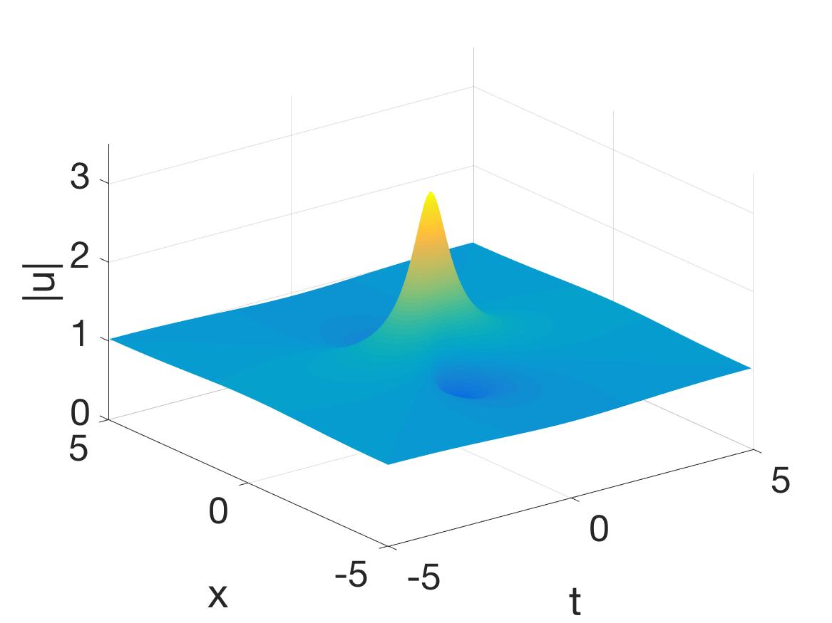
(a) $\nu=0$

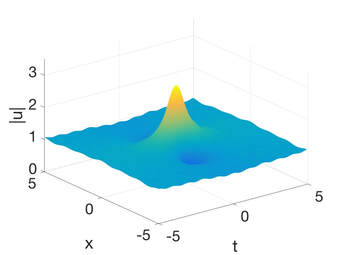
(b) $\nu=0.1$

(c) $\nu=0.15$

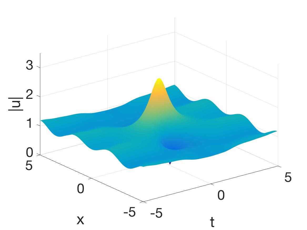
(d) $\nu=0.2$

Figure 3: Continuation over increasing $\nu$ values of the KM breather solution of the NLS. Note that the solution seems to transition into a breather on top of a periodic background as the nonlocality parameter is increased.

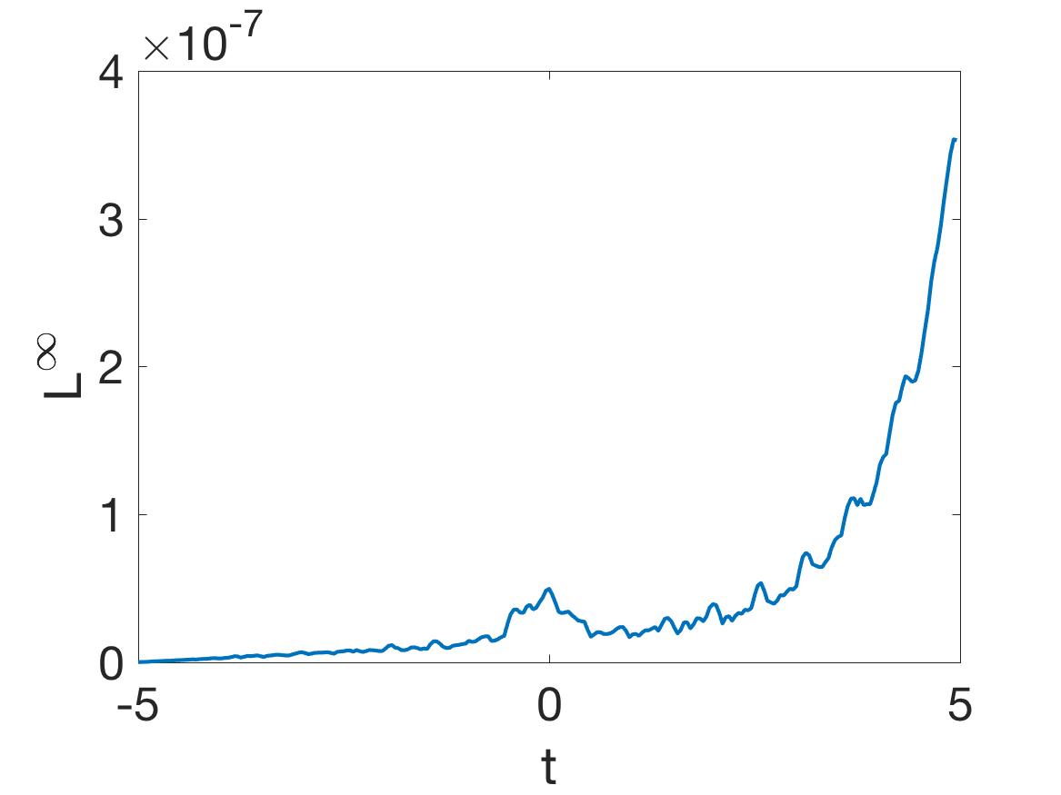
(a) $\nu=0$

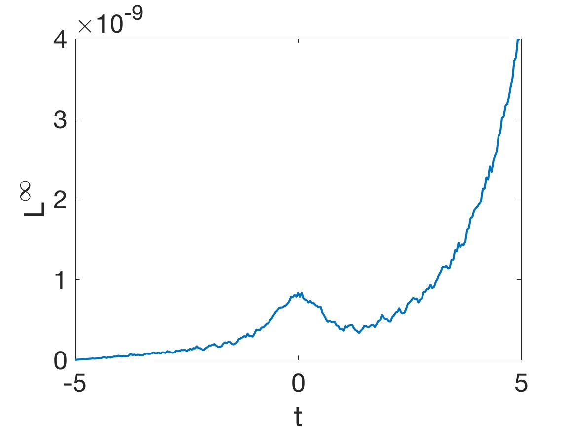
(b) $\nu=0.1$

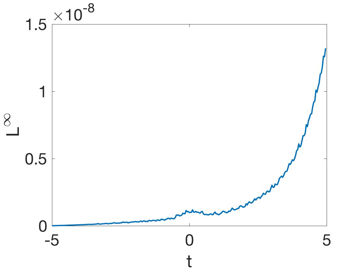
(c) $\nu=0.15$

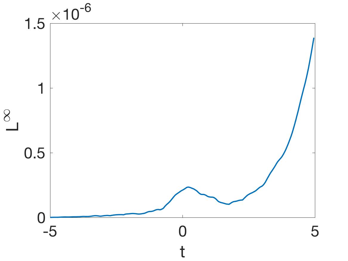
(d) $\nu=0.2$

Figure 4: $L^{\infty}$ error between the solution obtained by the Newton-CG method (as shown in Fig. 3) vs the solution obtained via the ETDRK4 method when the KM breather profile is seeded into the latter as an initial condition.

In this subsection, we present similar diagnostics for the KM breather waveform of Eq. (5). It is interesting that, here, the background modulation becomes more transparent and arises in the clear form of a progressively more intense (as the nonlocality parameter $\nu$ increases) periodic background. The resulting waveforms at $\nu=0.15-0.2$ are strongly reminiscent of the rogue waves on a periodic (i.e., elliptic function) background recently discovered in integrable models such as the nonlinear Schrödinger peli1 and the modified Korteweg-de Vries peli2 models. While such solutions have not previously been found, to the best of our knowledge, in the nonlocal model these results are strongly suggestive that they exist. Whether they can be identified in this nonintegrable model in some closed form remains an outstanding problem for future study. We should note here that the KM waveform can only be continued up to around $\nu=0.25$, but not beyond that.

The verification of the accuracy of the numerical solution is given in Fig. 4, in a way similar to what was done before in Fig. 2. Indeed, in this case the error up to $t=5$ does not grow in all the cases considered beyond O$(10^{-6})$. The associated growth observed in the ETDRK4 simulations initialized with the KM initial condition can be attributed to the exponential instability of the background seeded by the residual numerical error that eventually will grow to lead to deviations of O$(1)$ at sufficiently long times (propagation distances).

III.3 First Doubly Periodic Solution

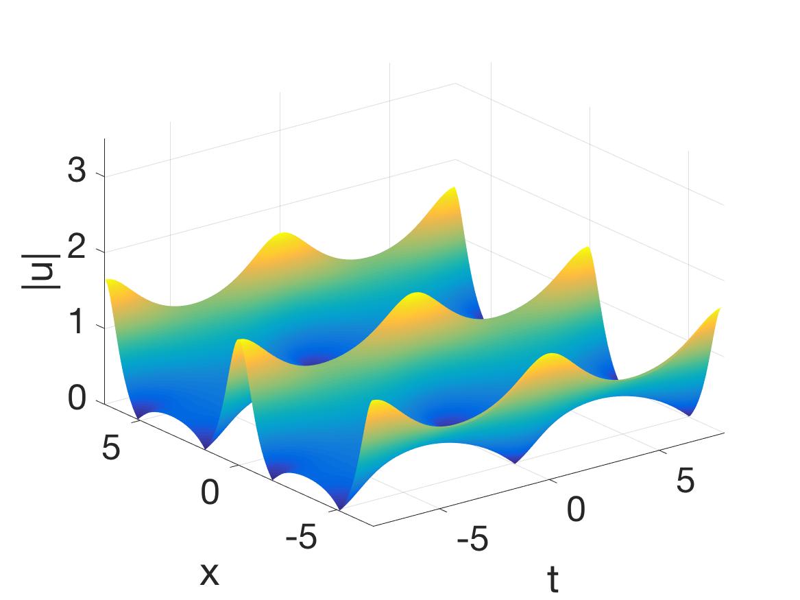
(a) $\nu=0$

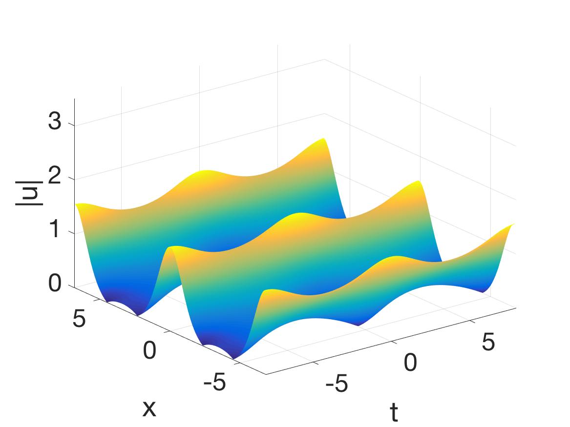
(b) $\nu=0.5$

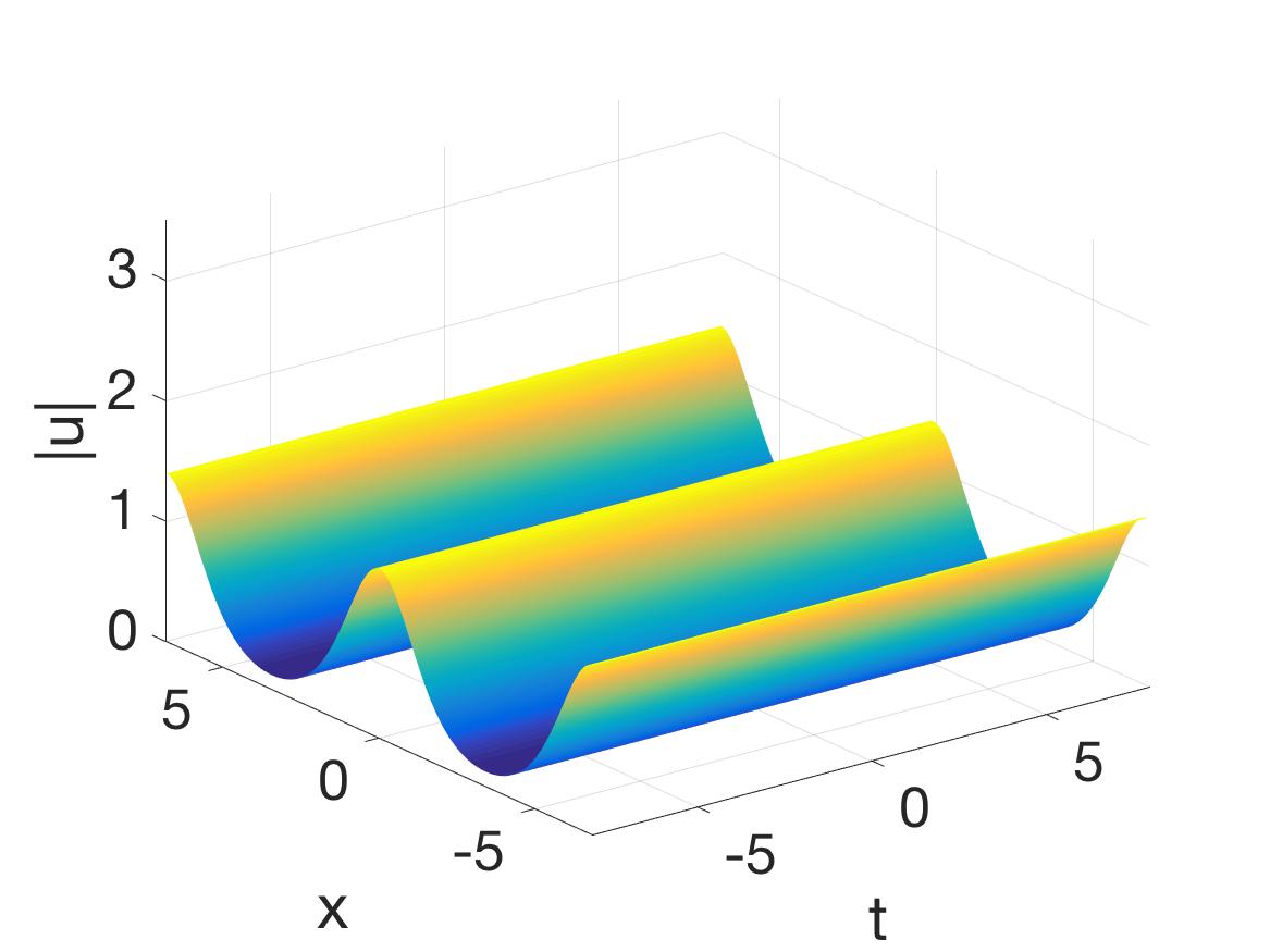
(c) $\nu=1$

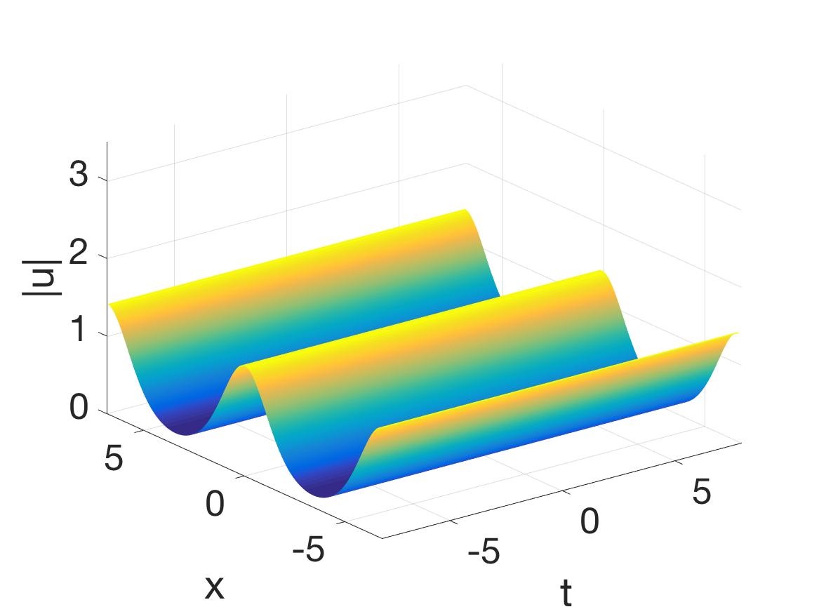
(d) $\nu=1.5$

Figure 5: Continuation over increasing $\nu$ values of the doubly periodic first solution of the NLS. It is seen that the doubly periodic solution bifurcates into a solution whose (modulus) profile is stationary and thus time-independent as $\nu$ is increased.

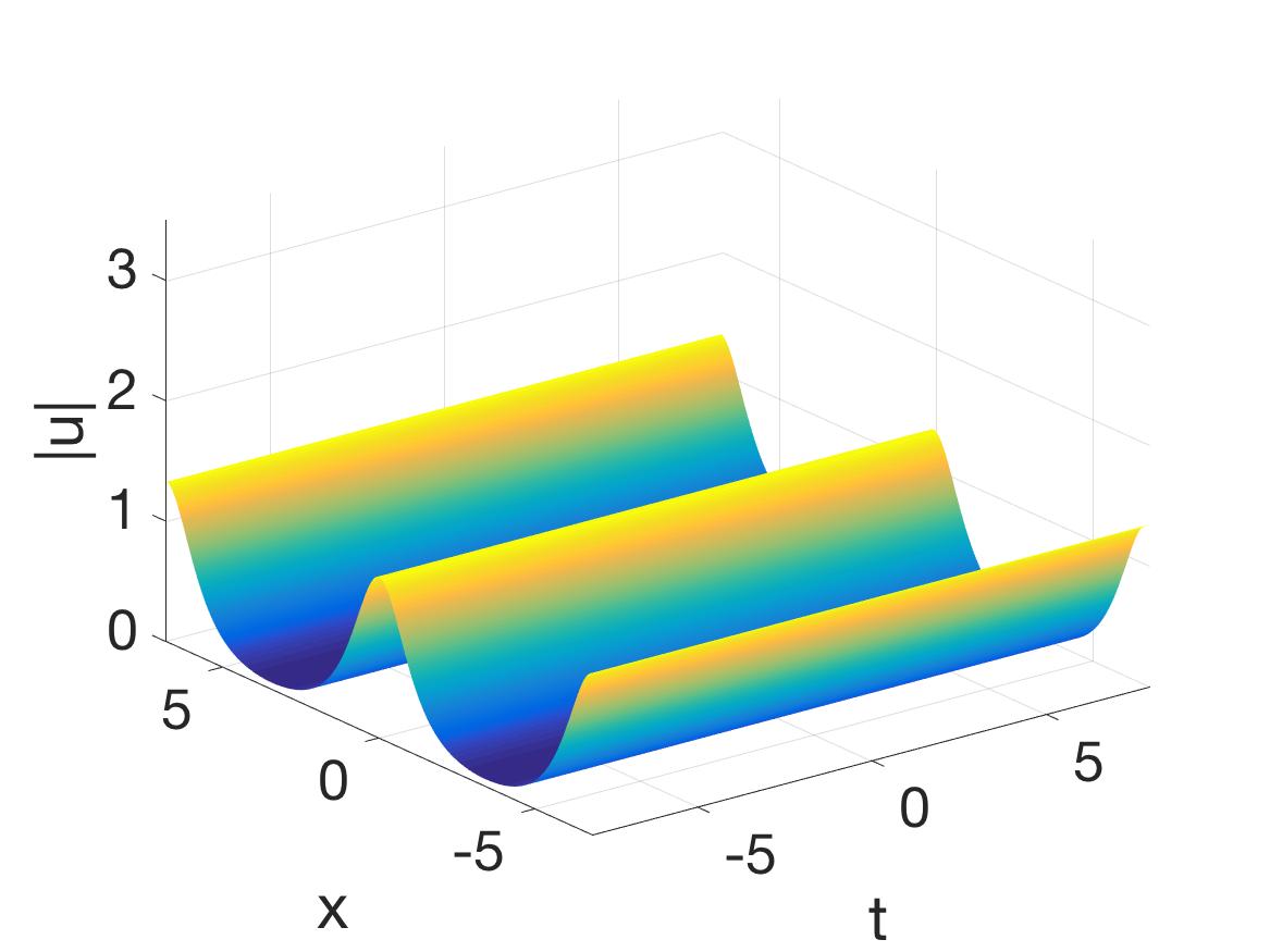
(a) $\nu=0$

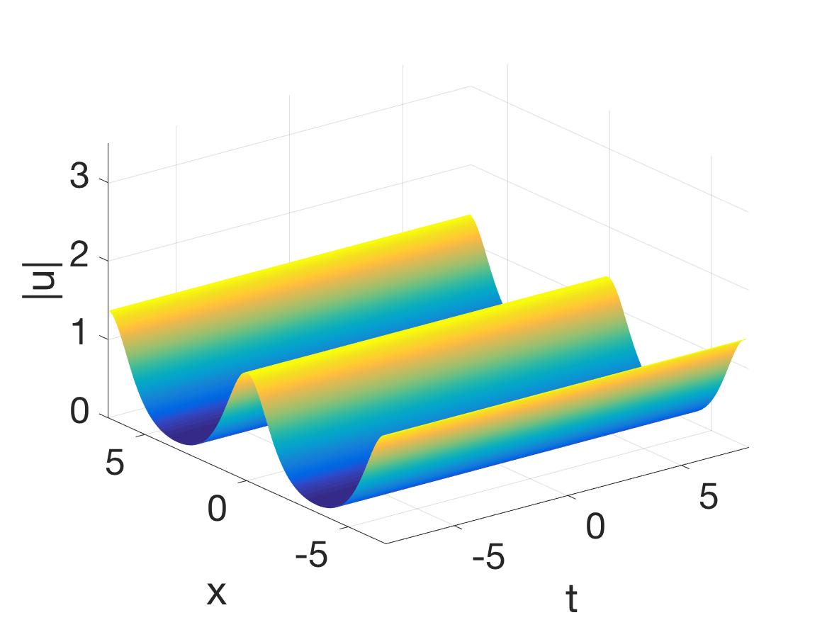
(b) $\nu=0.5$

(c) $\nu=1$

(d) $\nu=2$

Figure 6: Convergence to the stationary, periodic in space solution, obtained upon using as initial condition the solution in Fig. 5(e), and decrease of $\nu$. This periodic solution apparently exists all the way to the local NLS limit.

We now turn to the doubly periodic solution Eq. (7) for which the results are presented in Figs. 5-8; here we have chosen $\kappa=0.8$. As can be seen in Fig. 5, the amplitude of the solution is initially doubly periodic in both space and time but gradually, as the nonlocality parameter is increased, becomes singly periodic in space. By this we mean that the modulus of the solution becomes time-independent (i.e., we exclude phase factors that can be eliminated by means of a gauge transformation).

This naturally suggests the question of whether this stationary, periodic in space solution of the nonlocal problem emerges only in the nonlocal model or exists in the local limit. Indeed, continuing the stationary solution “downward” (i.e., for decreasing $\nu$) one can see that it bifurcates from a stationary (elliptic function) solution at the local NLS limit, given explicitly by

$$u=\exp(i\frac{\alpha t}{T})\;A\;\text{dn}\big{(}Ax,\sqrt{2+\frac{2\alpha-1}{A^{2}}}\big{)}$$ (9)

where $\alpha=\frac{2\pi}{T}$ and $A\approx 1.43$. The case examples of this state (for the same values of $\nu$ as in Fig. 5) are shown in Fig. 6. Indeed, the relevant bifurcation diagram illustrating the merger of the space-time periodic solution with the space-periodic one is shown in Fig. 7. The emergence of a solution with a finite periodicity from a stationary one suggests a Hopf scenario in the Hamiltonian system at hand.

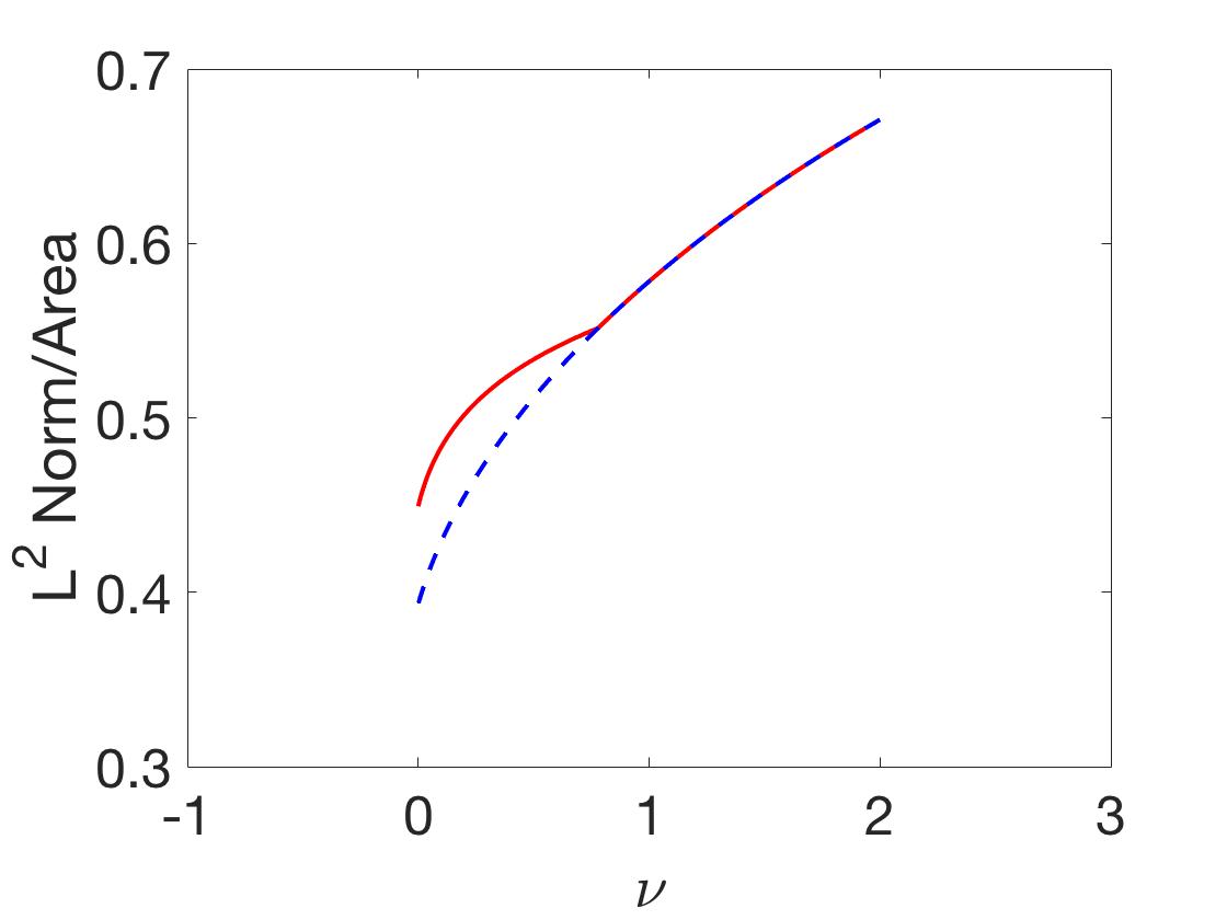
(a)

Figure 7: Bifurcation diagram showing the doubly periodic solution (solid) and the constant profile solution (dashed) as $\nu$ varies. Clearly, as $\nu$ increases the two branches merge with each other, i.e., the periodic (in time) orbit emerges from the stationary solution.

Lastly, here too, we examine the growth of the residual and find it to be very small ($(10^{-8})$ at the highest), when considering this class of solutions for different $\nu$’s even up to $\nu=2$ (for which the solution is stationary). The relevant results are presented in Fig. 8 for the periodic solution in time (that turns stationary as $\nu$ is increased). We show prototypical examples for the space-time periodic solution in panels (a)-(b), then for higher values of $\nu$ where the waveform acquires a stationary modulus in (c)-(d). Also for completeness, in panels (e)-(f) we go back down to lower values of $\nu$ along the branch of solutions of stationary modulus (i.e., periodic only in space) and examine the error in this case as well, confirming that it remains quite small during the evolution interval considered.

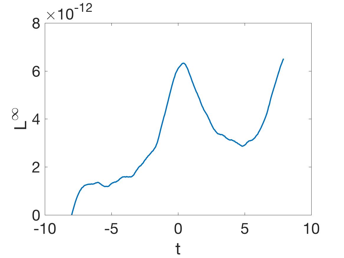
(a) $\nu=0$

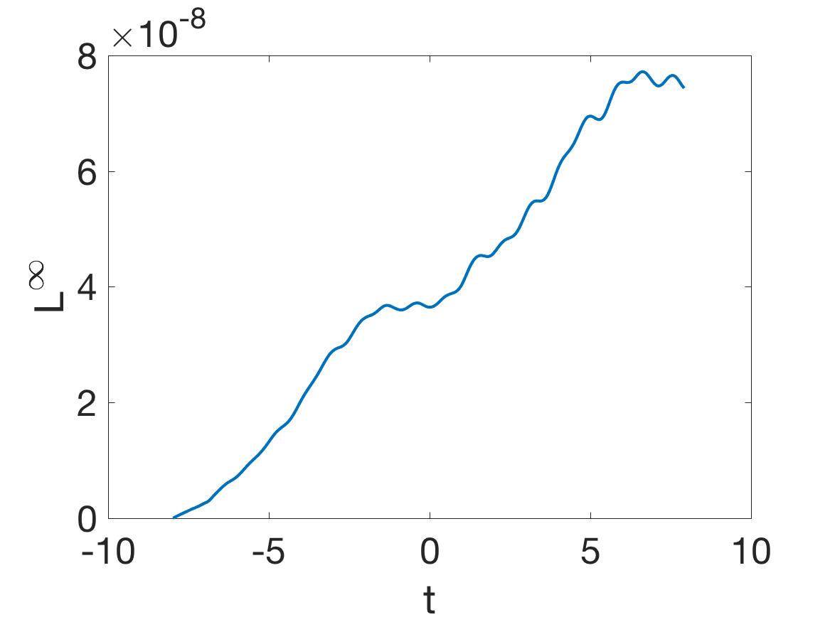
(b) $\nu=0.5$

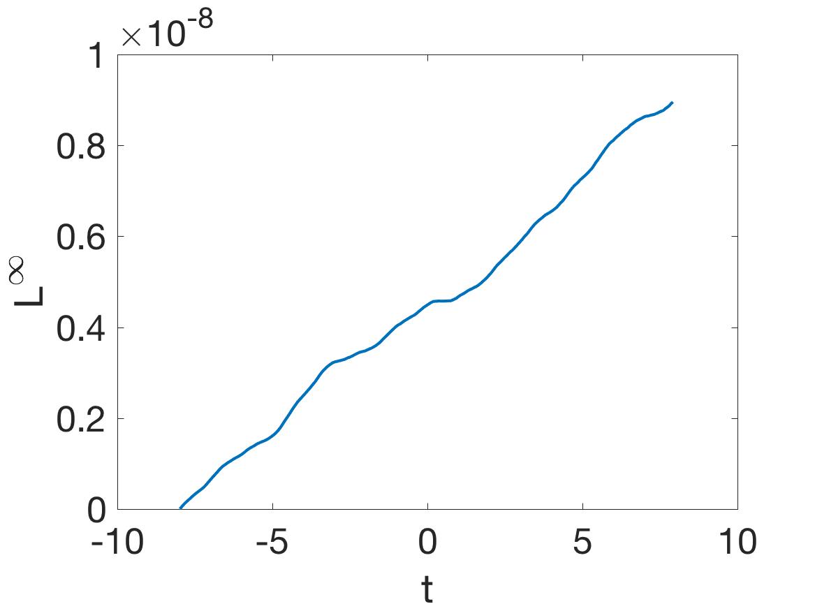
(c) $\nu=1$

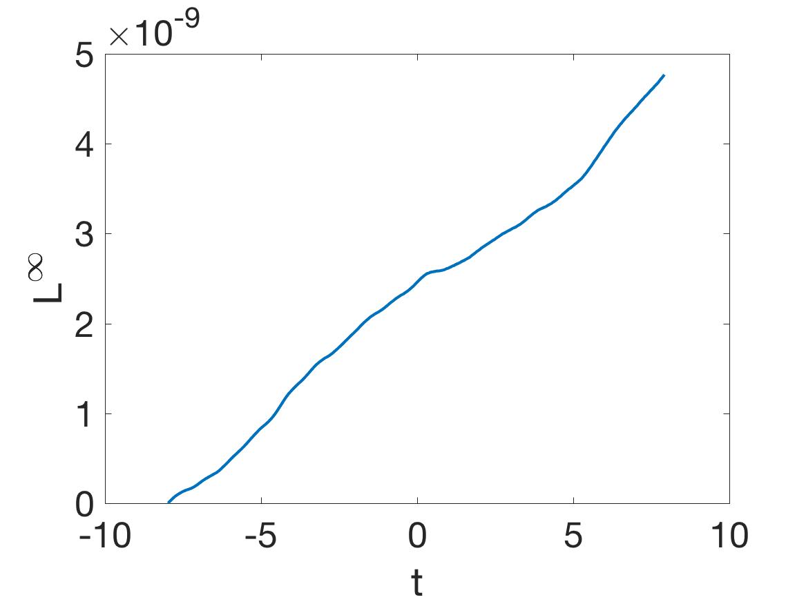
(d) $\nu=2$

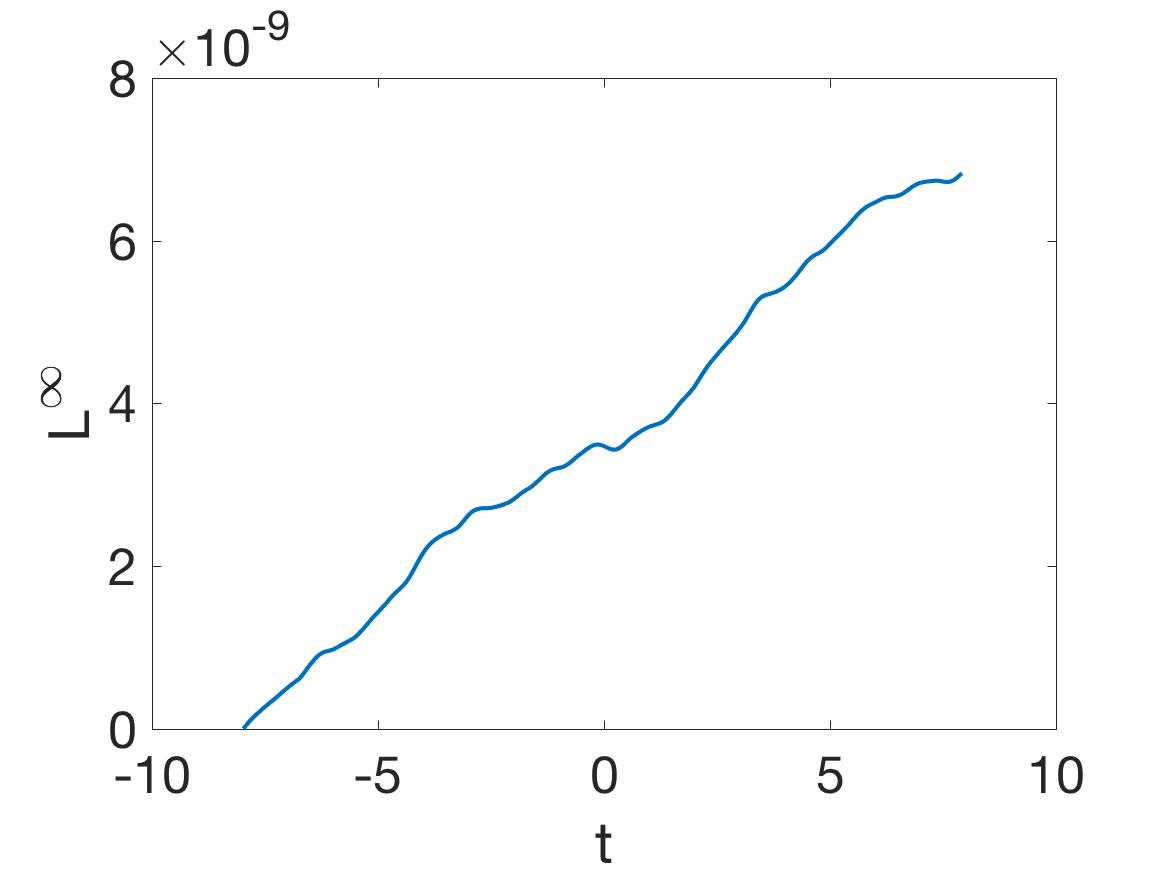
(e) $\nu=0.5$

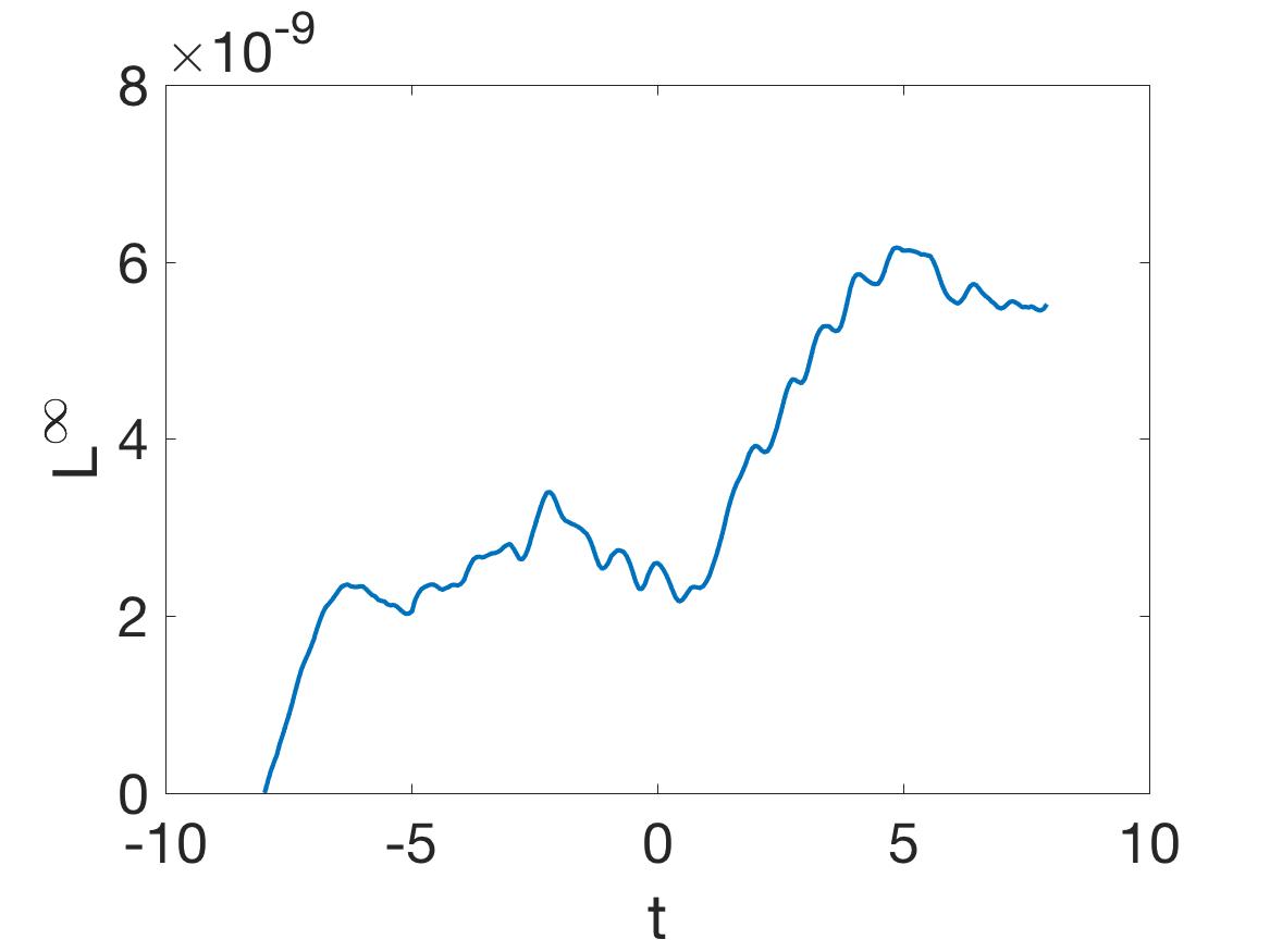
(f) $\nu=0$

Figure 8: $L^{\infty}$ error between the solution obtained by the Newton-CG method (as shown in Fig. 5) vs the solution obtained via the ETDRK4 method. Different values of $\nu$ up to $\nu=2$ are shown. Recall that in panels (c)-(f) the solution is, in fact, stationary. In panels (e)-(f) the error is shown for the solutions continued back down to lower values of $\nu$ along the branch of stationary (periodic in space) modulus.

III.4 Second Doubly Periodic Solution

In a similar vein, we now examine the continuation of the local solution Eq. (8) to the nonlocal regime. We find a similar phenomenology as a result of the continuation as in the previous section. Namely, the doubly periodic solution, as $\nu$ is increased, turns to a singly periodic one in the case of sufficiently large $\nu$; see Fig. 9. On the other hand, starting at $\nu=2$ and continuing the stationary (modulus) solution down to $\nu=0$, we find that the relevant waveform exists for all $\nu$ down to the local limit, as illustrated in Fig. 10.That is to say, there is again a bifurcation diagram Fig. 11 illustrating the Hopf type emergence of the periodic (in time) orbit from the stationary one (for decreasing $\nu$).

An additional interesting observation is that this stationary solution in the NLS limit ($\nu=0$) degenerates to an explicit cnoidal solution in the form of

$$u(x)=A\;\text{cn}\left(\sqrt{-1+2A^{2}}\;x,~{}\sqrt{\frac{2A^{2}}{2(-1+2A^{2})}}\right),$$ (10)

with $A\approx 1.62$. Further, we can also arrive at an exact expression for the stationary state as $\nu\to\infty$. Inspired by the numerics, we can judiciously guess a solution of the form

$$\begin{cases}u=A\cos(Bx),\\ \theta=C\cos(Dx)+E,\end{cases}$$

and use it in Eq. (2). Doing so, and matching terms, one gets conditions on the constants, namely

$$B=\frac{D}{2},\quad E=\frac{A^{2}}{2},\quad C=\frac{\beta}{2}\frac{A^{2}}{D^{2}+\beta},$$

where $\beta=\frac{2}{\nu}$. Equivalently,

$$\begin{cases}u=A\cos(\frac{D}{2}x)\\ \theta=\frac{\beta}{2}\frac{A^{2}}{D^{2}+\beta}\cos(Dx)+\frac{A^{2}}{2}.\end{cases}$$

Plugging this into the LHS of Eq. (1) and simplifying yields

$$i\frac{\partial u}{\partial t}+\frac{1}{2}\frac{\partial^{2}u}{\partial x^{2}}+\theta u-\frac{1}{2}u$$

$$=-\Big{(}\frac{D^{2}}{8}+\frac{1}{2}-\frac{A^{2}}{2}\Big{)}A\cos\left(\frac{D}{2}x\right)+\Big{(}\frac{\beta A^{2}}{2}\frac{A}{D^{2}+\beta}\Big{)}\cos(Dx)\cos\left(\frac{D}{2}x\right).$$ (11)

Taking $\beta\to 0$, or equivalently $\nu\to\infty$, the above reduces to $-\big{(}\frac{D^{2}}{8}+\frac{1}{2}-\frac{A^{2}}{2}\big{)}A\cos\left(\frac{D}{2}x\right)$ which we can make zero provided we choose

$$\frac{D^{2}}{8}+\frac{1}{2}-\frac{A^{2}}{2}=0.$$

This has two consequences. The first is that, as $\nu\to\infty$, we have the exact solution:

$$\begin{cases}u=A\cos(\sqrt{A^{2}-1}x)\\ \theta=\frac{A^{2}}{2}\end{cases}$$

The second, related one, is that under the limit $\nu\to\infty$ the nonlocal NLS reduces to the following linear Schrödinger equation:

$$\frac{1}{2}\frac{\partial^{2}u}{\partial x^{2}}+\frac{A^{2}}{2}u-\frac{1}{2}u=0.$$

From the bifurcation diagram in Fig. 11, as $\nu$ increases, we have found that the amplitude of $u$ approaches the constant value of $A\approx 1.92$.

It is relevant to remark here that the numerically obtained periodic in space solution is well approximated by the above asymptotic functional form. At $\nu=6$ the pointwise error between the two is approximately $2\times 10^{-2}$. In fact, our numerical observations suggest that one can approximate the numerically obtained periodic in space solution by the functional form:

$$u=A\text{cn}(Bx,C)$$

for suitably chosen $A,B,C$. In fact, with this approximation, the pointwise error can be made between $10^{-3}$ and $10^{-6}$ for all $\nu$ in the interval $0\leq\nu\leq 6$. This suggests the possibility of seeking suitable elliptic function solutions as potentially exact waveforms of the nonlocal model. This merits a separate investigation beyond the confines of the present work. Lastly, we note that for both branches of solutions, we present the diagnostic of the $L^{\infty}$ norm of the deviation from the numerically identified solution when propagating the corresponding initial condition with ETDRK4 in Fig. 12. This is similar to Fig. 8 with the top panels pertaining to the space-time periodic branch, while the bottom ones arise for the stationary modulus, periodic in space branch present for large $\nu$, but which can be continued down to lower values of $\nu$. Once again the relevant residual grows due to the instability of the background, yet remains bounded by $10^{-8}$ over the time scales considered.

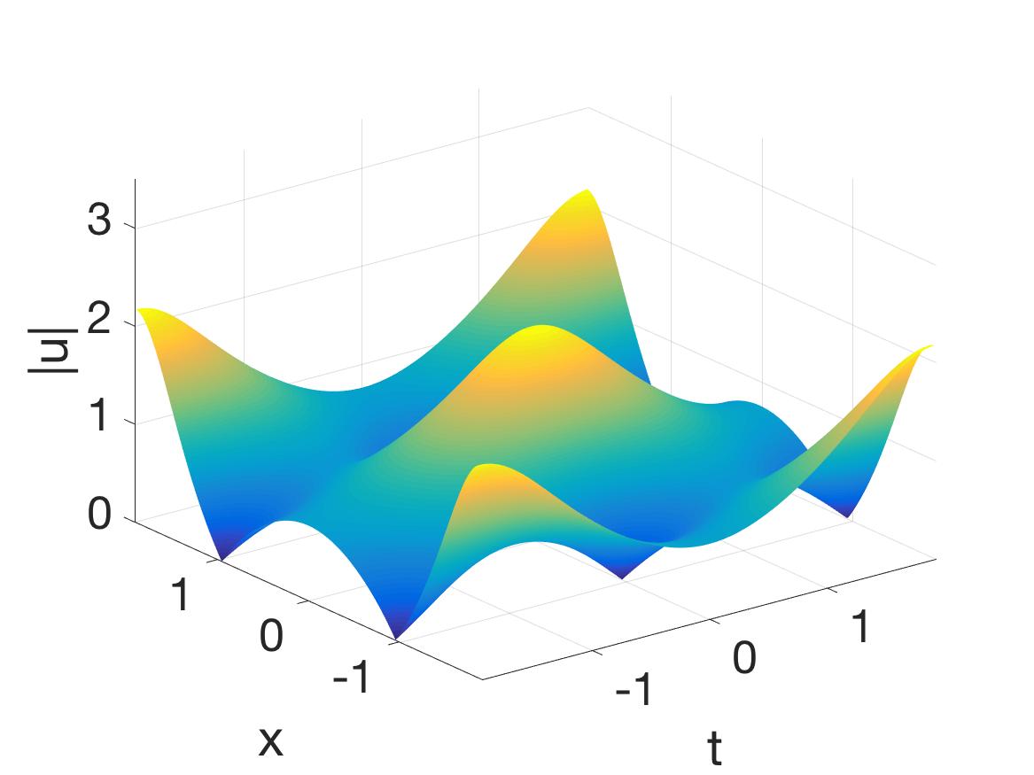
(a) $\nu=0$

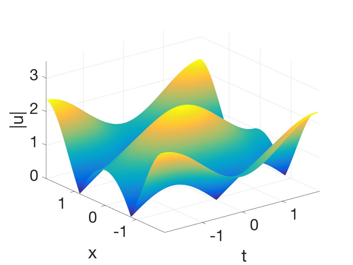
(b) $\nu=1.5$

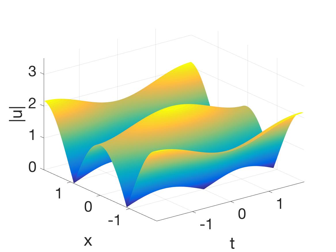
(c) $\nu=3$

(d) $\nu=6$

Figure 9: Continuation over increasing $\nu$ values of the second doubly periodic solution of the NLS. It is seen that the doubly periodic solution bifurcates into a solution whose profile is constant in time as $\nu$ is increased.

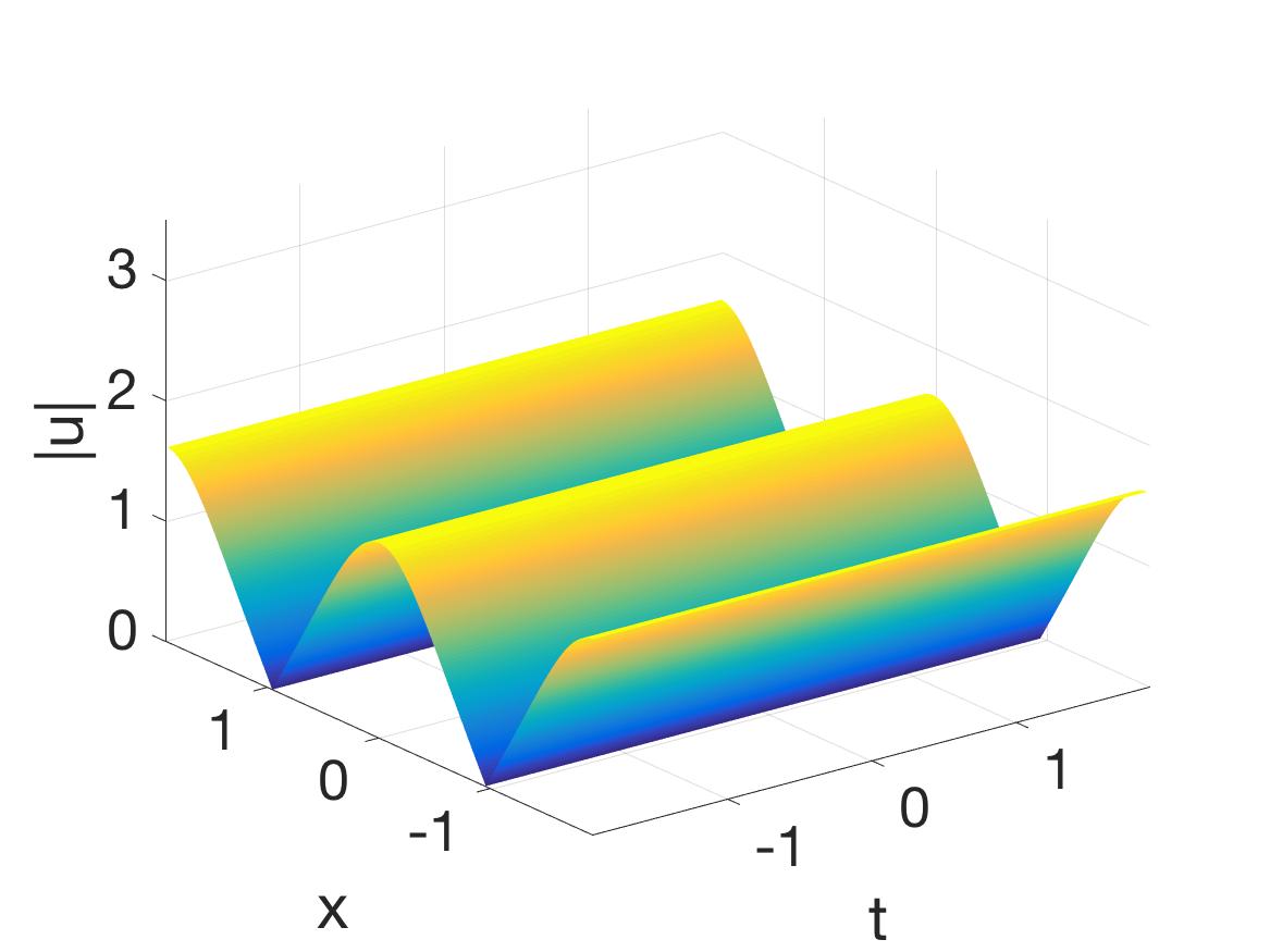
(a) $\nu=0$

(b) $\nu=1.5$

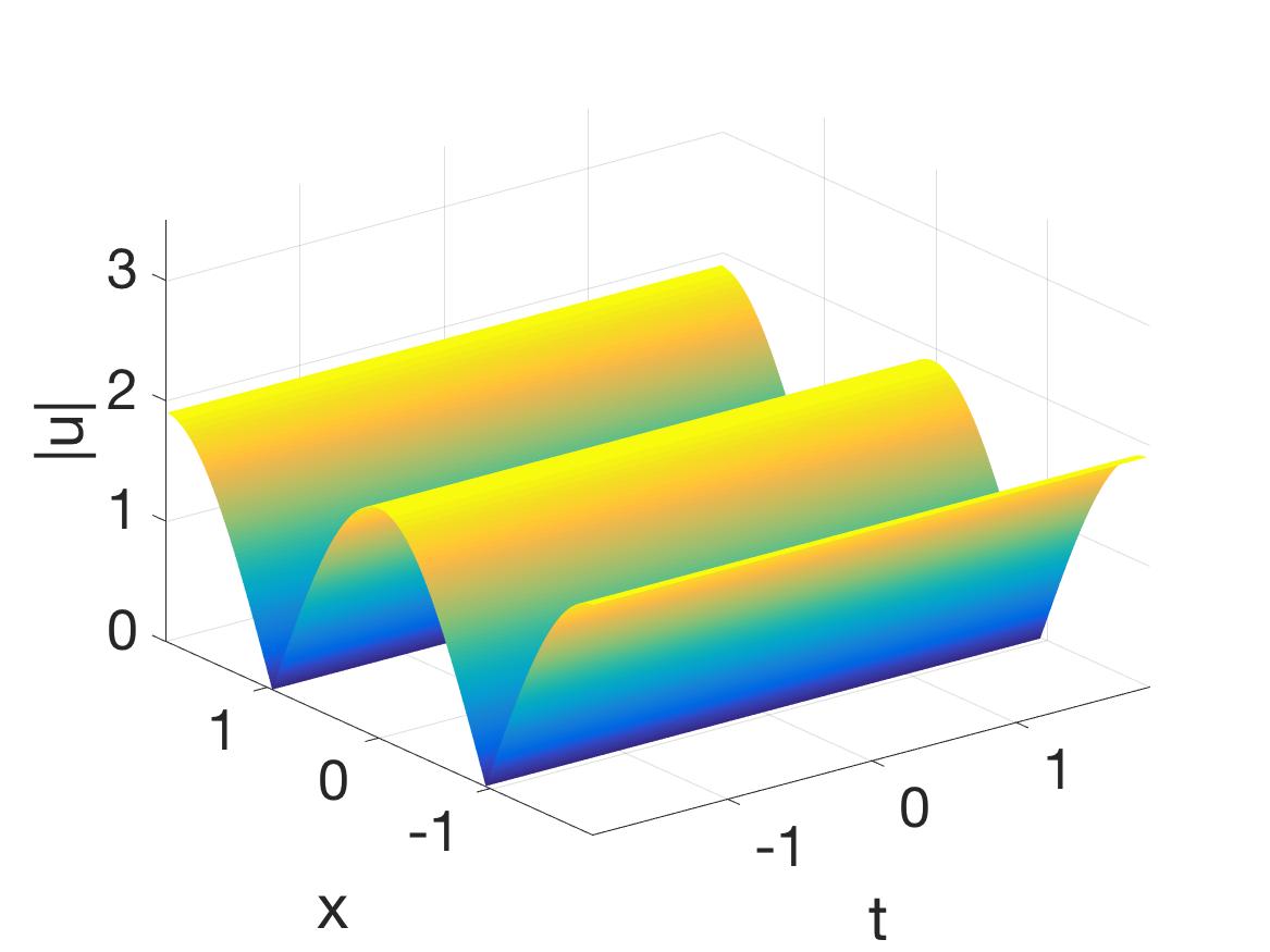
(c) $\nu=3$

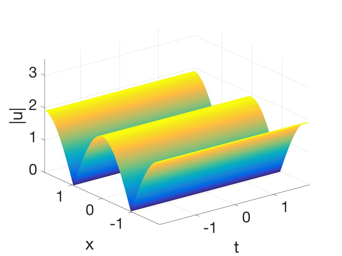
(d) $\nu=6$

Figure 10: Using as initial condition the solution in Fig. 9(e), we decrease $\nu$ and find the continuation of the stationary branch down to the NLS limit of $\nu=0$.

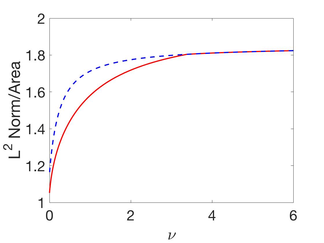
(a)

Figure 11: Bifurcation diagram showing the second doubly periodic solution (solid) and the constant profile solution (dashed) as $\nu$ varies.

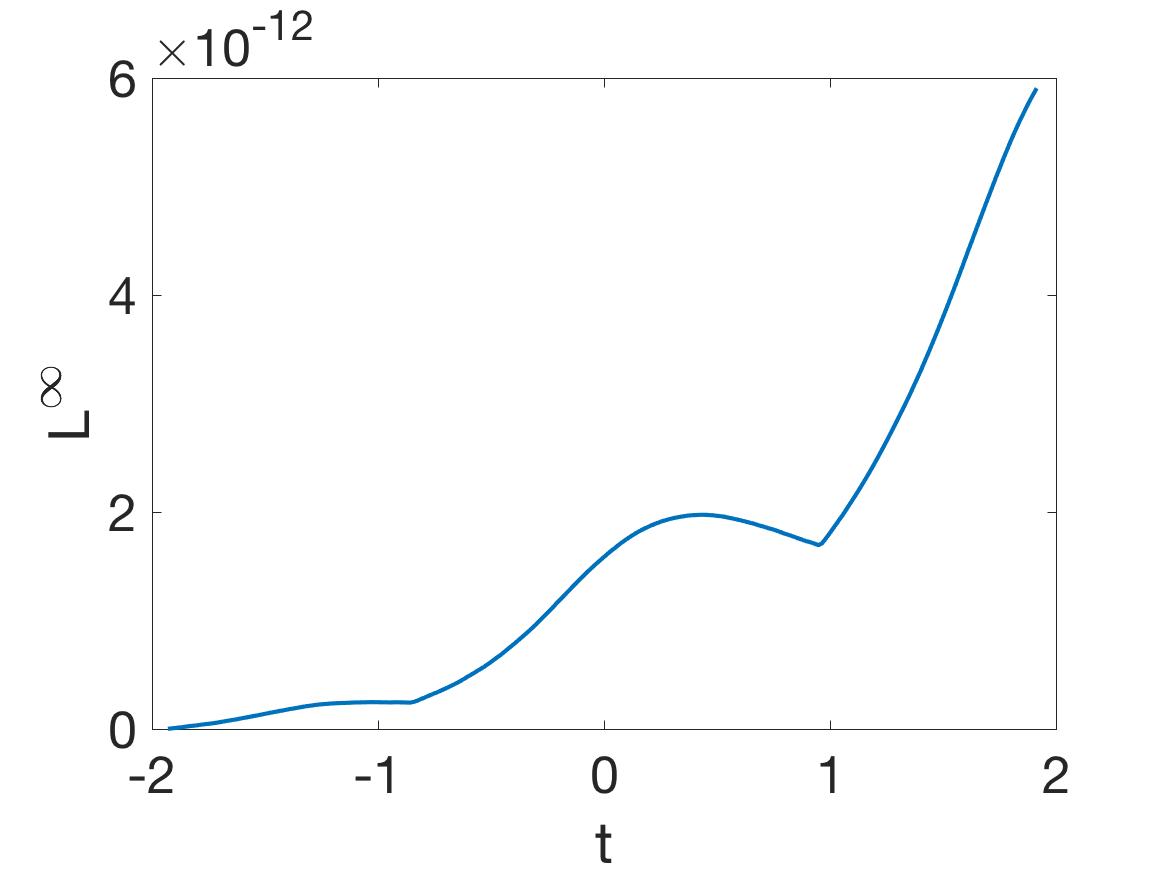
(a) $\nu=0$

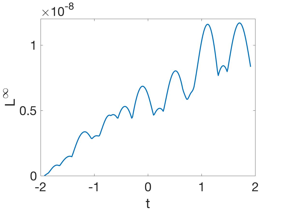
(b) $\nu=1.5$

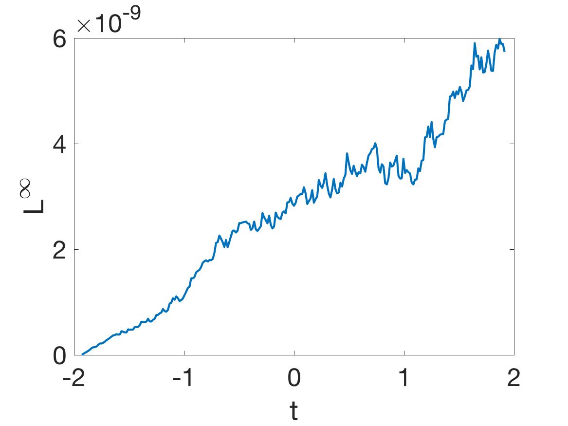
(c) $\nu=3$

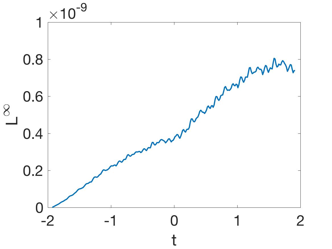
(d) $\nu=6$

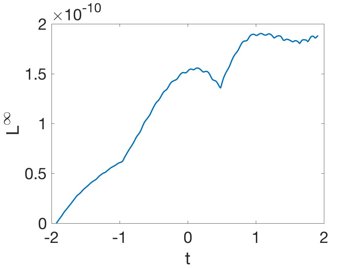
(e) $\nu=1.5$

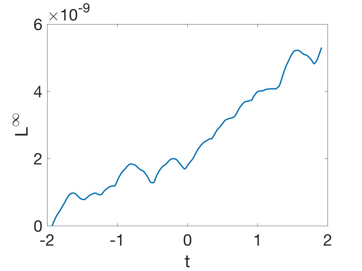
(f) $\nu=0$

Figure 12: $L^{\infty}$ error between the solution obtained by the Newton-CG method (as shown in Fig. 9) vs the solution obtained via the ETDRK4 method. The 3 top panels correspond to the error of the space time periodic solution, while the bottom 3 case examples are examples of the error in the evolution of waveforms of the stationary modulus branch.

IV Conclusions and Future Work

In the present work, we considered a variety of wave structures existing in the local NLS equation and extended them to the realm of a generic nonlocal NLS model. In this vein, we examined the prototypical rogue wave state, namely the Peregrine soliton, as well as its periodic in time generalization, the Kuznetsov-Ma (KM) breather. We also looked at other states that are periodic in both space and time, motivated by the work of akh . These continuations led to a number of interesting conclusions. Both the Peregrine soliton and the KM breather were possible to continue for small values of the nonlocality parameter $\nu$. This is appealing because it suggests that the structures are not particular to the integrable limit and can, indeed, be continued in the non-integrable case. Additionally, as the structures are continued they develop undulations which, in some cases (e.g., the KM state), suggest connections with other states that have been recently identified in integrable models, namely rogue waves mounted on elliptic function, spatially periodic structures. As regards the doubly-periodic states with periodicities in both space and time, these were more robustly identified through our continuation scheme and could, in fact, be continued up to $\nu=2$ and beyond. However, here too, there exists an interesting twist, namely the structures beyond a certain degree of nonlocality lost their temporal periodicity and became genuinely stationary in their modulus, maintaining only the spatial periodicity. These spatially periodic states were subsequently continued downward all the way to the local NLS limit, confirming their cnoidal nature in the latter and revealing the bifurcation of their spatiotemporally periodic counterparts.

We believe that these results offer considerable insight on the potential of the nonlocal model to support states (including rogue wave ones) with non-vanishing asymptotics, i.e., ones beyond the more “standard” solitary wave ones. However, additionally, they also motivate a number of further questions and inquiries worth considering in future studies. One of these is whether stationary elliptic function solutions can be suitably generalized in analytically available waveforms in the nonlocal case (or whether these can only be identified in limiting cases such as the ones of $\nu\rightarrow 0$ and $\nu\rightarrow\infty$ considered herein). Another topic of interest is to explore systematically continuations of the newly discovered rogue waves on periodic wave background and explore how such structures may generalize in the case of the nonlocal model. Possibly these may be involved in bifurcation phenomena associated with the states considered here. Another more open ended challenge is whether rogue-wave-like patterns, such as the Peregrine soliton or the KM breather, can be continued beyond the intervals of $\nu$ for which they were found herein in the case of the nonlocal model. Lastly, in the present study we focused chiefly on the existence and in some cases on the bifurcations of the solutions. However, there are stability tools gradually emerging (such as, e.g., the Floquet analysis of the KM state and the consideration of the Peregrine as a limiting case of that calculation PRE ) that would be quite relevant to consider in the present nonlocal setting as well. Potential progress in any of these directions will be reported in future publications.

References

- (1) W. Krolikowski, O. Bang, N. I. Nikolov, D. Neshev, J. Wyller, J. J. Rasmussen, and D. Edmundson, J. Opt. B: Quantum Semiclass. Opt. 6, S288 (2004).
- (2) G. Assanto, A.A. Minzoni, N.F. Smyth, J. Nonlin. Opt. Phys. Mat. 18, 657 (2009).
- (3) G. Assanto, Nematicons: Spatial Optical Solitons in Nematic Liquid Crystals Wiley-Blackwell (New Jersey, 2012).
- (4) C. Rotschild, O. Cohen, O. Manela, M. Segev, and T. Carmon, Phys. Rev. Lett. 95, 213904 (2005).
- (5) C. Conti, M. Peccianti, and G. Assanto, Phys. Rev. Lett. 91, 073901 (2003).
- (6) A. G. Litvak, V. A. Mironov, G. M. Fraiman, and A. D. Yunakovskii, Sov. J. Plasma Phys. 1, 60 (1975).
- (7) A. I. Yakimenko, Y. A. Zaliznyak, and Y. S. Kivshar, Phys. Rev. E 71, 065603(R) (2005).
- (8) T.P. Horikis, D.J. Frantzeskakis, Phys. Rev. Lett. 118 (2017) 243903.
- (9) T. P. Horikis, D.J. Frantzeskakis, Proc. Roy. Soc. A 475, 20190110 (2019).
- (10) P. Pedri and L. Santos, Phys. Rev. Lett. 95, 200404 (2005).
- (11) M. J. Edmonds, T. Bland, D. H. J. O’Dell, and N. G. Parker, Phys. Rev. A 93, 063617 (2016).
- (12) A. Dreischuh, D.N. Neshev, D.E. Petersen, O. Bang, and W. Krolikowski Phys. Rev. Lett. 96, 043901 (2006).
- (13) M. Shen, J.-J. Zheng, Q. Kong, Y.-Y. Lin, C.-C. Jeng, R.-K. Lee, and W. Krolikowski Phys. Rev. A 86, 013827 (2012).
- (14) B. K. Esbensen, M. Bache, O. Bang, and W. Krolikowski Phys. Rev. A 86 033838 (2012).
- (15) N.Akhmediev, A.Ankiewicz, M.Taki, Phys. Lett. A 373, 675 (2009).
- (16) A. Chabchoub, N. P. Hoffmann, and N. Akhmediev, Phys. Rev. Lett. 106, 204502 (2011).
- (17) A. Chabchoub, N. Hoffmann, M. Onorato, and N. Akhmediev, Phys. Rev. X 2, 011015 (2012).
- (18) A. Chabchoub and M. Fink, Phys. Rev. Lett. 112, 124101 (2014).
- (19) D. R. Solli, C. Ropers, P. Koonath, and B. Jalali, Nature 450, 1054 (2007).
- (20) B. Kibler, J. Fatome C. Finot, G. Millot, F. Dias, G. Genty, N. Akhmediev, J.M. Dudley, Nature Phys. 6, 790 (2010) .
- (21) B. Kibler, J. Fatome, C. Finot, G. Millot, G. Genty, B. Wetzel, N. Akhmediev, F. Dias and J. M. Dudley, Sci. Rep. 2, 463 (2012).
- (22) J. M. Dudley, F. Dias, M. Erkintalo, and G. Genty, Nat. Photon. 8, 755 (2014).
- (23) B. Frisquet, B. Kibler, P. Morin, F. Baronio, M. Conforti, G. Millon, S. Wabnitz, Sci. Rep. 6, 20785 (2016).
- (24) C. Lecaplain, Ph. Grelu, J. M. Soto-Crespo, and N. Akhmediev, Phys. Rev. Lett. 108, 233901 (2012).
- (25) A. N. Ganshin, V. B. Efimov, G. V. Kolmakov, L. P. Mezhov-Deglin, and P. V. E. McClintock, Phys. Rev. Lett. 101, 065303 (2008).
- (26) H. Bailung, S. K. Sharma, and Y. Nakamura, Phys. Rev. Lett. 107, 255005 (2011).
- (27) M. Onorato, S. Residori, U. Bortolozzo, A. Montina, and F. T. Arecchi, Phys. Rep. 528, 47 (2013).
- (28) P. T. S. DeVore, D. R. Solli, D. Borlaug, C. Ropers, and B. Jalali, J. Opt. 15, 064001 (2013).
- (29) Z. Yan, J. Phys. Conf. Ser. 400, 012084 (2012).
- (30) N. Akhmediev et al., J. Opt. 18, 063001 (2016).
- (31) S. Chen, F. Baronio, J. M. Soto-Crespo, P. Grelu, and D. Mihalache, J. Phys. A: Math. Theor. 50, 463001 (2017).
- (32) D. Mihalache, Rom. Rep. Phys. 69, 403 (2017).
- (33) B. A. Malomed and D. Mihalache, Rom. J. Phys. 64, 106 (2019).
- (34) E. Pelinovsky and C. Kharif (eds.), Extreme Ocean Waves, Springer-Verlag (New York, 2008).
- (35) C. Kharif, E. Pelinovsky, and A. Slunyaev, Rogue Waves in the Ocean, Springer-Verlag (New York, 2009).
- (36) A. R. Osborne, Nonlinear Ocean Waves and the Inverse Scattering Transform, Academic Press (Amsterdam, 2010).
- (37) M. Onorato, S. Residori, and F. Baronio, Rogue and Shock Waves in Nonlinear Dispersive Media, Springer-Verlag (Heidelberg, 2016).
- (38) B. Yang, J. Yang, Lett. Math. Phys. 109, 945 (2019).
- (39) M.J. Ablowitz, Z.H. Musslimani, Phys. Rev. Lett. 110, 064105 (2013).
- (40) T.P. Horikis, M.J. Ablowitz, Phys. Rev. E 95, 042211 (2017).
- (41) C.B. Ward, P.G. Kevrekidis, N. Whitaker, Phys. Lett. A 383, 2584 (2019).
- (42) D. H. Peregrine, J. Austral. Math. Soc. B 25, (1983) 16–43.
- (43) E.A. Kuznetsov, Sov. Phys.-Dokl. 22 (1977) 507–508.
- (44) Ya.C. Ma, Stud. Appl. Math. 60 (1979) 43–58.
- (45) N.N. Akhmediev, V.M. Eleonskii, and N.E. Kulagin, Exact first-order solutions of the nonlinear Schrödinger equation, Theor. Math. Phys. 72, 809 (1987).
- (46) A.-K. Kassam and L. N. Trefethen, SIAM J. Sci. Comput. 26, 1214 (2005).
- (47) J. Chen, D.E. Pelinovsky, R.E. White, arXiv:1905.11638.
- (48) J. Chen, D.E. Pelinovsky, arXiv:1807.11361.
- (49) J. Cuevas-Maraver, P. G. Kevrekidis, D. J. Frantzeskakis, N. I. Karachalios, M. Haragus, and G. James, Phys. Rev. E 96, 012202 (2017).