Learning Point Embeddings from Shape Repositories for Few-Shot Segmentation

Abstract

User generated 3D shapes in online repositories contain rich information about surfaces, primitives, and their geometric relations, often arranged in a hierarchy. We present a framework for learning representations of 3D shapes that reflect the information present in this meta data and show that it leads to improved generalization for semantic segmentation tasks. Our approach is a point embedding network that generates a vectorial representation of the 3D points such that it reflects the grouping hierarchy and tag data. The main challenge is that the data is noisy and highly variable. To this end, we present a tree-aware metric-learning approach and demonstrate that such learned embeddings offer excellent transfer to semantic segmentation tasks, especially when training data is limited. Our approach reduces the relative error by $10.2\%$ with $8$ training examples, by $11.72\%$ with $120$ training examples on the ShapeNet semantic segmentation benchmark, in comparison to the network trained from scratch. By utilizing tag data the relative error is reduced by $12.8\%$ with $8$ training examples, in comparison to the network trained from scratch. These improvements come at no additional labeling cost as the meta data is freely available.

1 Introduction

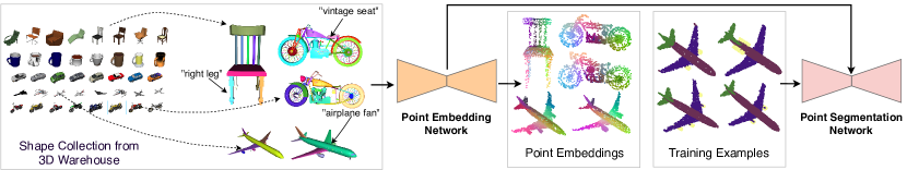
Figure 1: Overview of our approach. Shape collections in 3D shape repositories contain metadata such as polygon groupings and tags assigned to parts. These parts and tags assigned to them are highly variable, even within the same category. We use the shapes and metadata to train a point embedding network that maps each point into a fixed dimensional vector (see Section 4 and Figure 3 for details.) The embeddings for a few shapes are visualized as color channels using t-SNE mapping, where similar colors indicate correspondence across shapes. The learned parameters when used to initialize a point segmentation network leads to improved performance when few training examples are available. (Please zoom in for details.)

The ability to decompose a 3D shape into semantic parts can enable applications from shape retrieval in online repositories, to robotic manipulation and shape generation. Yet, automatic techniques for shape segmentation are limited by the ability to collect labeled training data, which is often expensive or time consuming. Unlike images, online repositories of user-generated 3D shapes, such as the 3D Warehouse repository [2], contain rich metadata associated with each shape. These include information about geometric primitives (e.g., polygons in 3D meshes) organized in groups, often arranged in a hierarchy, as well as color, material and tags assigned to them. This information reflects the modeling decisions of the designer are likely correlated with high-level semantics.

Despite its abundance, the use of metadata for learning shape representations has been relatively unexplored in the literature. One barrier is the high degree of its variability. These models were created by designers with a diverse set of goals and with a wide range of expertise. As a result the groups and hierarchies over parts of a shape that reflect the modeling steps taken by the designer are highly variable: two similar shapes can have significantly different number of parts as well as the number of levels in the part hierarchy. Moreover, the tags are rarely assigned to parts and are often arbitrarily named. Figures 1 and 2 illustrate this variability.

Our work systematically addresses these challenges and presents an approach to exploit the information present in the metadata to improve the performance of a state-of-the-art 3D semantic segmentation model. Our approach, illustrated in Figure 1, consists of a deep network that maps each point in a 3D shape to a fixed dimensional embedding. The network is trained in a way such that the embedding reflects the user-provided hierarchy and tags. We propose a robust tree-aware metric to supervise the point embedding network that offers better generalization to semantic segmentation tasks over a baseline scheme that is tree-agnostic (only considers the leaf-level groupings). The point embedding network trained on hierarchies also improves over models trained on shape reconstruction tasks that leverage the 3D shape geometry but not their metadata. Finally, when tags are available we show that the embeddings can be fine-tuned leading to further improvements in performance.

On the ShapeNet semantic segmentation dataset, an embedding network pre-trained on hierarchy metadata outperforms a network trained from scratch by reducing relative error by $10.2\%$ across 16 categories, when trained on $8$ shapes per category. Similarly, when only a small fraction of points (20 points) per shape are labeled, the relative reduction in error is $4.9\%$. Furthermore, on 5 categories which have sufficient tags, using both the hierarchy and tags reduces error further by $12.8\%$ points relative to the randomly initialized network, when trained on $8$ shapes per category. Our visualizations indicate that the trained networks implicitly learn correspondences across shapes.

2 Related Work

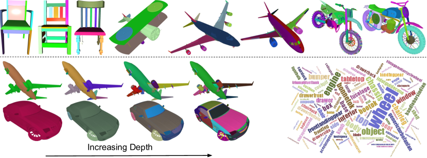
Figure 2: (Top row) Example shapes from our dataset. Our dataset consist of shapes segmented into parts without any semantic information. Notice that shapes of same category can be segmented differently from each other. Here different color represents different leaf node in the part-hierarchy. (Bottom left) Parts at different depths of the hierarchy for an airplane and a car. Increasing the depth increases the number and granularity of parts. (Bottom right) A word cloud of raw tags collected from our dataset. The font size is proportional to the square root of frequency of the dataset.

Our work builds on the advances in deep learning architectures for point-based, or local, shape representations and metric learning approaches to guide representation learning. We briefly review relevant work in these areas.

Supervised learning of local shape descriptors.

Several architectures have been proposed to output local representations, or descriptors, for 3D shape points or patches. The architectures can be broadly categorized according to the type of raw 3D shape representation they consume. Volumetric methods learn local patch representations by processing voxel neighborhoods either in uniform [15] or adaptively subdivided grids [20, 14, 24, 25]. View or multi-view approaches learning local image-based representations by processing local 2D shape projections [9, 23], which can be mapped back onto the 3D shape [12]. Finally, a large number of architectures have been recently proposed for processing raw point clouds. PointNet and PointNet++ are transforming individual point coordinates and optionally normals through MLPs and then performing permutation-invariant pooling operations in local neighborhhoods [18, 19].

All the above-mentioned deep architectures are trained in a fully supervised manner using significant amound of labeled data. Although for some specific classes, like human bodies, these annotations can be easily obtained through template-based matching or synthetically generated shapes [3, 4, 5], for the vast majorities of shapes in online repositories, gathering such annotations often requires laborious user interaction [16, 30]. Active learning methods have also been proposed to decrease the workload, but still rely on expensive crowdsourcing [30].

Weak supervision for learning shape descriptors.

A few methods [17, 31] have been recently proposed to avoid expensive point-based annotations. Muralikrishnan et al. [17] extracts point-wise representations by training an architecture designed to predict shape-level tags (e.g., armrest chair) by first predicting intermediate shape segmentations. Instead of using weak supervision in the form of shape-level tags, we use unlabeled part hierarchies available in massive online repositories and tags for parts (not whole shapes) when such are available. Yi et al. [29] embeds pre-segmented parts in descriptor space by jointly learning a metric for clustering parts, assigning tags to them, and building a consistent part hierarchy. In our case, our architecture learns point-wise descriptors and also relaxes the requirement of inferring consistent hierarchies, which might be hard to estimate for shape families with significant structural variability. Non-rigid geometric alignment has been used as a form of weak and noisy supervision by extracting approximate local shape correspondences between pairs of shapes of similar structure [11] or by deforming part templates [10]. However, global shape alignment can fail for shapes with different structure, while part-based alignment requires corresponding parts or definition of part templates in the first place. In a concurrent work, given a collection of shapes from a single category, Chen et al. [6] proposed a branched autoencoder that discovers coarse segmentations of shapes by predicting implicit fields for each part. Their network is trained with a few manually selected labeled shapes in a few-shot semantic segmentation setting. Our method instead utilizes part hierarchies and metadata as weak supervisory signal. We also randomly select labeled sets for our few-shot experiments. In general, our method is complementary to all the above-mentioned weak supervision methods. Our weak signal in the form of unlabeled part hierarchies and part tags can be used in conjunction with geometric alignment, consistent hierarchies, or shape-level tags, whenever such are possible to obtain.

Triplet-based metric learning.

Our approach learns a metric embedding over points that reflects the hierarchies in 3D shape collections. Metric learning has a rich literature with a diverse applications and techniques. A popular approach is to supervise the learning with “triplets” of the form $(a,b,c)$ to denote that “a is more similar to b than c”. This can be written as $d(a,b)\leq d(a,c)$ where the $d(a,b)$ denotes the distance between $a$ and $b$. The distance itself could be computed as the Euclidean distance in some embedding space, i.e., $d(a,b)=||\phi(a)-\phi(b)||_{2}$, possibly computed with a deep network. Within this framework, techniques to sample triplets remains an active area of research. These include techniques such as hard-negative mining [7], semi-hard negative mining [21] and distance weighted sampling [28] to bias the sampling of triplets.

3 Mining Metadata from Shape Repositories

We first describe the source of our part hierarchy dataset that we use for training our embedding network. Then we describe the metadata (tags) present in the 3d models and how we extract this information into a consistent dataset.

Part hierarchies.

Several 3D modeling tools, such as SketchUp, Maya, 3DS Max to name a few, allow users to model shapes, and scenes, in general, as a collection of geometric entities (e.g., polygons) organized into groups. The groups can be nested and organized in hierarchies. In our part hierarchy dataset, we endeavor to extract these hieararchies. The shapes in our dataset are a subset of Shapenet Core dataset, where we focus on $16$ categories from Shapenet part-segmentation dataset [30] to allow systematic benchmarking and comparison with prior work. Note that the $16$ categories semantic segmentation dataset contains $~{}16.6k$ shapes, whereas $16$ categories in Shapenet Core dataset contains $~{}28k$ shapes. We first retrieved the original files for shapes in Shapenet Core dataset provided by 3d warehouse, which are stored in the popular “COLLADA” format [26]. These files represent 3D models in a hierarchical tree structure. Leaf nodes represent shape geometry, and internal nodes represent groups of geometric primitives, or nested groups. Samples from our dataset are visualized in the Figure 2. Number of parts in which a shape is segmented depends on the part-hierarchy as visualized in the Figure 2 (bottom left). Models with too few part segmentation (less than $2$) or too many (more than $500$) are discarded. This gives us a total of $20776$ 3D models having part group information, with each model having at least one level of part grouping. We further segment the dataset into train ($15625$), validation ($3113$) and test ($2038$) splits. We ensure that the shapes in test split of semantic part-segmentation dataset [30] are not included in the train split of our part hierarchy dataset.

Category	Shapes with part tagged	Avg points tagged
Motorcycle	$110$	$11.3\%$
Airplane	$806$	$5.0\%$
Table	$392$	$45.7\%$
Chair	$326$	$38.7\%$
Car	$600$	$20.0\%$

Table 1: Dataset with tags. Number of shapes with at least one tagged parts, and average percentage of points tagged in these shapes in 5 categories.

Tag extraction.

Modeling tools allow users to explicitly give tags to parts, which are stored in their corresponding file format. Obviously, not all designers enter tags for their designed parts. Out of all the models that include part group information in our dataset, we observed that only $10.7\%$ of the shapes had meaningful tags for at least one part (i.e., tags are sparse). Usually, these tags are not consistent, e.g., a tag for a wheel part in a car can be “wheel_mesh”. To make things worse, few tags have high frequency e.g., one may encounter wheel, chassis, windows (or synthetics of those) frequently as tags, while most of them are rare, or even be non-informative for part types e.g., “geometry123”.

To extract meaningful tags, we selected the $10$ most frequent tags encountered as strings, or sub-strings stored in the nodes for each shape category. We also merge synonyms into one tag to reduce number of tags in the final set. For every tag, we find the corresponding geometry nodes and then we label the points sampled from these nodes with the tag. We found that only $5$ out of $16$ categories have a “sufficient” number of tagged points ($>1\%$ of the original surface points). By “sufficient”, we mean that below this threshold, tags are becoming so sparse in a category that result in negligible improvements. Table 1 shows the distribution of tags in these $5$ categories.

Geometric postprocessing.

We finally aligned the shapes using ICP so that their orientation agrees with the canonical orientation provided for the same shapes in ShapeNet. To process the shapes through our point-based architecture, we uniformly sampled 10K points on their surface. Further details about these steps are provided in the supplementary material.

4 Method

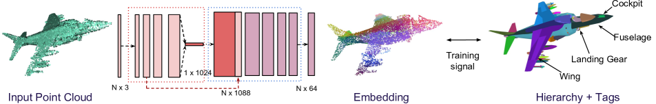
Figure 3: Architecture of the Point Embedding Network (PEN). The network takes as input a point cloud and outputs a fixed dimensional embedding for each point, visualized here using t-SNE. These embeddings are learned using metric learning that utilizes part-hierarchy. Furthermore, embedding can be improved by supervising network using sparsely tagged point cloud from a small subset of our dataset (refer Table 1). Tags are pointed by arrows.

Our Point Embedding Network (PEN) takes as input a shape in the form of a point cloud set, $X=\{\mathbf{x}_{i}\}_{i=1}^{N}$, where $\mathbf{x}$ represents the 3D coordinates of each point. Our network learns to map each input shape point $\mathbf{x}$ to an embedding $\phi_{\mathbf{w}}(\mathbf{x})\in{\cal R}^{d}$ based on learned network parameters $\mathbf{w}$. The architecture is illustrated in Figure 3. PEN first incorporates a PointNet module [18]: the points in the input shape are individually encoded into vectorial representations through MLPs, then the resulting point-wise representations are aggregated through max pooling to form a global shape representation. The representation is invariant to the order of the points in the input point set. At the next stage, the learned point-wise representations are concatenated with the global shape representation, and are further transformed through fully-connected layers and ReLUs. In this manner, the point embeddings reflect both local and global shape information.

We used PointNet as a module to extract the initial point-wise and global shape representation mainly due to its efficiency. In general, other point-based modules, or even volumetric [15, 24, 20] and view-based modules [22, 9] for local and global shape processing could be adapted in a similar manner within our architecture. Below we describe the main focus of our work to learn the parameters of the architecture based on part hierarchies and tag data.

Learning from part hierarchies.

Our training takes a standard metric learning approach where the parameters of the PEN are optimized such that pairs originating from the same part sampled from the hierarchy (positive pairs) have distance smaller than pairs of points originating from different parts (negative pairs) in the embedded space. Specifically, given a triplet of points $(a,b,c)$, the loss of the network over this triplet [8] is defined as:

$$\ell(a,b,c)=\big{[}d(a,b)-d(a,c)+m\big{]}_{+},$$ (1)

where $d(a,b)=\left\lVert\phi_{w}(a)-\phi_{w}(b)\right\rVert_{2}^{2}$, $m$ is a scalar margin, and $[x]_{+}=\max(0,x)$. To avoid degenerate solutions we constrain the embeddings to lie on a unit hypersphere, i.e., $\left\lVert\phi(x)\right\rVert_{2}^{2}=1$, $\forall x$. Given a set of triplets ${\cal T}_{s}$ sampled from each shape $s$ from our dataset $S$, the triplet objective of the PEN is to minimize the triplet loss:

$$L_{triplet}=\sum_{s\in S}\frac{1}{|{\cal T}_{s}|}\sum_{(a,b,c)\in{\cal T}_{s}}\ell(a,b,c).$$ (2)

Sampling triplets.

One simple strategy to sample triplets is to just access the parts at the finest level of segmentation, then sample triplets by randomly taking fixed number of similar pairs $(a,b)$ from the same part and an equal number of negative points $c$ from another part. We call this strategy “leaf” triplet sampling.

An alternative strategy is to consider the part hierarchy tree for triplet sampling. Here, we sample negative point pairs depending on the tree distance between the part groups (tree nodes) they belong to. Given two nodes $n_{i}$ and $n_{j}$, we use the sum of path lengths (number of tree edges) from nodes $n_{i}$ and $n_{j}$ to their lowest common ancestor as the tree distance $\delta(n_{i},n_{j})$ [27] . For example, if the two nodes are siblings (i.e., two parts belonging to the same larger group), then their lowest common ancestor is their parent and their tree distance is equal to $2$ (i.e., count two edges that connect them to their parent). If two nodes are further away in the hierarchy, then tree distance increases. In this manner, the tree distance reflects how far two nodes (parts) are in the hierarchy.

We compute the probability of selecting the positive pair of points from node $n_{i}$ and the negative pair using the point from another node $n_{j}$ as follows:

$$P(n_{i},n_{j})\propto\frac{1}{\delta(n_{i},n_{j})}$$ (3)

Sampling points in this way yields more frequent triplets that consist of negative pairs closer in the hierarchy. Parts that are closer in the hierarchy tend to be spatially or geometrically closer to each other, thus also harder to discriminate. We call this sampling strategy as “hierarchy” triplet sampling. We discuss the effect of these two strategies in the experiments section.

Learning from noisy tag data.

We can also utilize tag data for segments collected from the COLLADA files, as described in Section 3. To train the network using tags, we add two pointwise fully-connected layers on top of the embedding network (PEN). One way to train this network is to define a categorical cross entropy over points whose parts are tagged. However, as shown in Table 1, the total number of tagged points is small. We instead found that a better strategy is to use a one-vs-rest binary cross entropy loss to also make use of points in un-tagged parts. The reason is that if a part is not tagged in a shape that has other parts labeled with tags existing in the shape metadata, then most likely, that part should not be labeled with any of the existing tags for that shape (e.g., if a car has tagged parts as ‘wheel’ and ‘window’, then other un-tagged parts should most likely not be assigned with these tags).

More specifically, for every tag in our tag set $\mathcal{L}$ for a shape category, we define a binary cross entropy loss by considering all points assigned with that tag as ‘positive’ (set $\mathcal{P}$) while the rest of points assigned with other or no tags as ‘negative’ (set $\mathcal{N}$). Given an output probability prediction for assigning a point $i$ with tag $t$, denoted as $P(y_{i,t}=1)$ produced by the last classification layer (sigmoid layer) of our network, our loss function over tags is defined as follows:

$$L_{tag}\!\!=\!-\!\sum_{t\in\mathcal{T}}\!\bigg{(}\sum_{i\in\mathcal{P}}\log P(y_{i,t}\!=\!1)+\sum_{i\in\mathcal{N}}\log(1-P(y_{i,t}\!=\!1))\bigg{)}$$ (4)

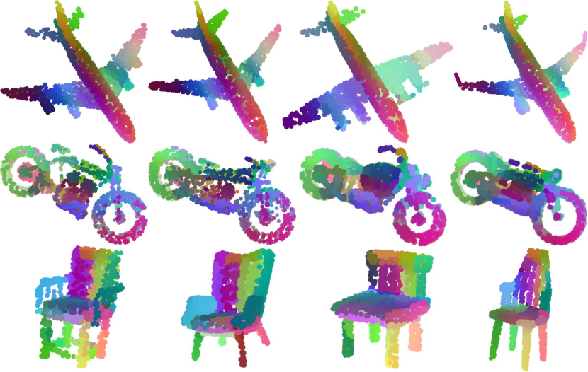
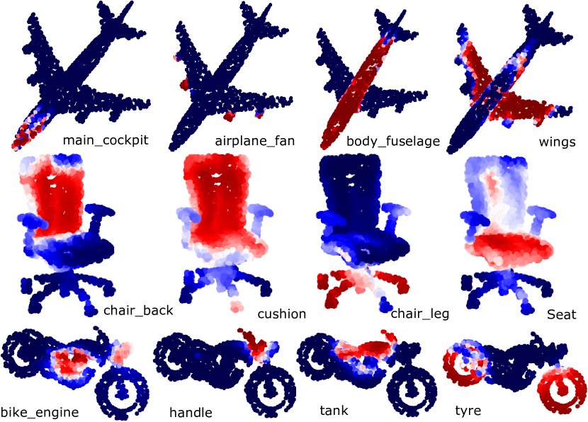
Figure 4: Visualization of the embeddings. (Left) T-SNE visualization of embedding shown as a color map. Embeddings for similar semantic parts are consistently embedded close to each other as reflected by the similarity in their color. (Right) Heat map visualization of tags predictions across a number of categories and tags. Redder values indicate a higher probability of the tag. (Best seen magnified.)

Training.

We first train our network to minimize the triplet loss $L_{triplet}$ based on our dataset of shapes that contains part hierarchies. Training is done in a cross-category manner on $16$ categories of ShapenetCore dataset, as described in Section 3. We use the Adam optimizer [13] with initial learning rate of $0.01$ decayed by the factor of $10$ whenever the triplet loss stops decreasing over validation set. The mini-batches consist of $32$ shapes. For further efficiency, in each iteration we randomly sample a subset of $2.5k$ points (from the $10K$ original points) for each shape during training. The total number of triplets sampled from a shape is kept constant.

Then for the $5$ categories that include tags, we further fine-tune the learned embeddings by learning the two additional pointwise fully-connected layer with a Sigmoid at the end to minimize the tag loss $L_{tag}$. Since tags are distinct for each category, fine-tuning is done in a category-specific manner (i.e., we produce a different embedding specialized for each of these $5$ categories). Although the triplet and tag loss could be combined, we choose a stage-wise training approach since the shapes with part hierarchies are significantly more numerous than the shapes that include tags as shown in Table 1. In our experiments we discuss the effect of training only with the triplet loss, and also the effect of fine-tuning with the tag loss in each category.

For training networks on few-shot learning task, we do hyper-parameters (batch size, epochs, regularization etc.) search using validation set of only one category (‘airplane’) and use the same hyper-parameters setting to train all models on all categories in the few-shot learning task.

Few-shot learning.

Given our network pre-trained on our shape datasets based on part hierarchies and/or tags, we can further train it on other, much smaller, datasets of shapes that include semantic part labels. To do this, once again we add two point-wise fully-connected layers on top of the embedding layer, and a softmax layer to produce semantic part label probabilities. In our experiments, we observe that the part labeling performance is significantly increased when compared to training our network from scratch using semantic part labels only as supervision.

Implementation details.

In our implementation, the encoder of our network extracts $1024$-dimensional global shape embedding. The decoder concatenates the global embedding with $64d$ point features from encoder, and finally transform it into a $64$-dimensional point-wise embeddings. Further details of the layers used in PEN are discussed in the supplementary material. Our implementation is based on PyTorch [1].

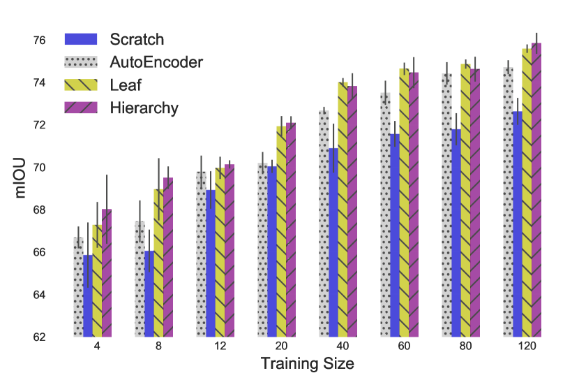
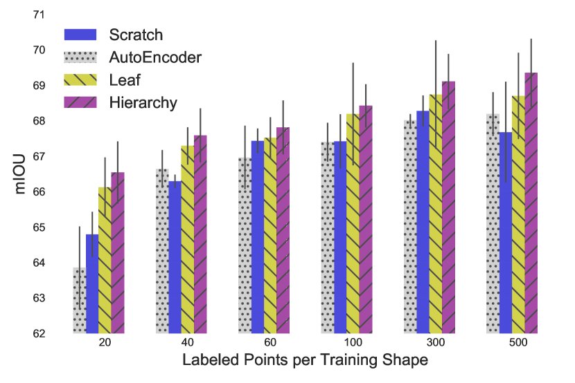
Figure 5: Benifits of pretraining PEN using metric learning. Left: mIoU evaluation for varying number of training shapes. Right: mIoU evaluation for varying number of labeled points and fixing the number of training shapes to $8$. We compare different baselines and variants of PEN, including training from scratch, autoencoder for pre-training, as well as PEN trained with metric learning triplets sampled from the leaf of the tree (Leaf) or based on the hierarchy (Hierarchy). PEN outperforms both baselines with the hierarchy-based sampling offering a slight advantage over the leaf-based one.

5 Results

We now discuss experiments performed to evaluate our method and alternatives. First, we present qualitative analysis of learned embeddings, then we discuss a new benchmark we introduce for few-shot segmentation and evaluation metrics, and finally we present results and comparisons of our network with various baselines.

Visualization of the embeddings.

We first present a qualitative analysis of the PEN embeddings. The embeddings learnt using metric learning only (without the tag loss) are visualized in Figure 4 (left). We use the t-SNE algorithm to embed the $64$-dimensional point embedding in $3D$ space. Interestingly, the descriptors produced by PEN consistently embed the points belonging to similar parts close to each other without explicit semantic supervision. We also visualize the embeddings predicted by PEN trained with metric learning and fine-tuned with tag loss in Figure 4 (right). The embeddings have better correspondence with the tags. Interestingly, the network predicts correct embeddings for points with tags that are not mutually exclusive e.g. ‘cushion’ and ‘back’ of the chair.

Few-shot Segmentation Benchmark.

We anticipate that learning from metadata can improve semantic shape segmentation tasks, especially in the few-shot learning scenario. To this end we have created a new benchmark on ShapeNet segmentation dataset [30], in which we randomly select $x$ fully labeled examples from the complete training set for training the network, where $x\in\{4,8,12,20,40,60,120\}$. In this manner, we can test the behaviour of methods with increasing training number of shapes, starting with the few-shot scenario where only a handful of shapes (i.e., 4 or 8) is labeled. The performance is measured as the mean intersection over union (mIOU) across all part labels and shapes in the test splits. We exclude the shapes existing in our part hierarchy and tag datasets used for pre-training PEN from the test splits.

We also introduce one more evaluation setting, where for each shape category, the training shapes have smaller fractions of their original points labeled ($20$, $40$ …$500$) labeled points compared to the original $2.5K$ points) The case of $\sim 20$-$40$ labeled point simulates the scenario where semantic annotations are collected through sparse user input (e.g., click few points on shapes and label them).

Figure 6: Benefit of training with tag supervision. The mIoU evaluation when tags are available (5 categories: motorcycle, airplane, table, chair, car). We include the same baselines and PEN variants as Figure 5, including two more PEN variants: one trained with tags only (Tags) and another trained both on hierarchy and tags (Hierarchy + Tags). Left: Shows the performance in the few-shot setting. Right: Shows the performance in the few-point setting. In both cases the tag data (Hierarchy + Tags) provides additional benefits over the PEN models trained with the hierarchy supervision (Hierarchy). Tag data alone is not as effective as the autoencoder since the supervision is highly sparse.

Baselines.

Since we utilize a vast number of unlabeled data from the same domain it is important to compare with baselines. Our first baseline simply trains PEN from scratch on the training splits of our few-shot segmentation benchmark using only semantic label supervision (without using metadata). Second, we also compare with another baseline, where we train an autoencoder network that leverages only geometry as an alternative to produce point-wise embeddings. This network first encodes the input point cloud to point-wise embeddings producing a $1024$-dimensional point-wise representations exactly as in PEN, then a decoder uses upconvolution to reconstruct the original point cloud. The Chamfer distance between generated points and input points is used as a loss function to train this network. We first pre-train the autoencoder on the shapes included in our part hierarchy dataset. After this pre-training step, we retain the encoder and replace the geometry decoder with PEN’s decoder and add two pointwise fully connected layers and a classification layer to produce semantic part label probabilities. The resulting network is then trained in stages, first the decoder and then the entire network at smaller learning rate, on the training splits of our few-shot segmentation benchmark.

Finally, we also evaluate the two strategies to pretrain the embedding network using different triplet sampling techniques i.e. leaf-level shape parts (“leaf” triplet sampling) and based on using the hierarchy tree (“hierarchy” triplet sampling) as described in (Section 4).

Next, we compare the performance of our method with the baselines and different sampling strategies under the scenario of using only the triplet loss and cross-category training. Then, we discuss the performance in the case where we additionally use the tag loss.

Few-shot Segmentation Evaluation.

In Figure 5 (left), we plot the mIOU of the baselines along with our method. The plotted mIOU is obtained by taking the average of the mIOU on our test splits over all categories and repeating each experiment $5$ times. The network trained from scratch (without any pre-training) has the worst performance. The network based on the pre-trained autoencoder shows some improvement since its point-wise representations reflect local and global geometric structure for the point cloud reconstruction, which can be also relevant to the segmentation task. Our method consistently outperforms the baselines. In particular, the “hierarchy” triplet sampling that uses the part hierarchy trees to choose triplets for training our network performs the best on average. A $3.5\%$ mIOU improvement ($10.2\%$ drop in relative error) is observed compared to training from scratch at $8$ training examples - interestingly, the improvement is retained even for $120$ training examples. The “hierarchy” triplet sampling also improves over the “leaf” triplet sampling until $20$ training examples, then their difference gap between these two strategies is closed.

Evaluating with limited labeled points per shape.

In the previous section we observed the performance of our method and baselines by changing the number of training shapes. Here we also examine the performance in the few-shot setting where we keep the number of training shapes fixed and vary the number of labeled points per training shape. We retrain the above baselines (train from scratch, autoencoder) and triplet sampling strategies (“leaf” and “hierarchy”) with $8$ training examples, and vary the number of labeled points as shown in the Figure 5 (right). Again our network using the “hierarchy” triplet sampling performs better than the baselines. It offers $1.7\%$ better mIOU ($4.9\%$ drop in relative error) compared to training from the scratch using $20$ labeled points.

Are tags useful?

Here we repeat the two few-shot sementation tasks on 5 shape categories (motorcycle, airplane, table, chair, car) that include some tagged parts in their shape metadata. Here, we examine two more PEN variants: (a) PEN pre-trained using the tag loss only (no triplet loss), then fine-tuned on the training splits of our semantic segmentation benchmark (this baseline is simply called “tags” network), 2) our network pre-trained using triplets loss based on the “hierarchy” sampling, then fine-tuned with the tag loss, and finally further fine-tuned on the training splits of our semantic segmentation benchmark (this baseline is called “Hierarchy+Tags” network). The two PEN variants are trained per each category of the $5$ categories. The results are shown in Figure 6.

When using $8$ training examples, the Hierarchy+Tags network offers $4.8\%$ better mIOU ($12.8\%$ drop in relative error) on average compared to training from scratch in these 5 categories (refer Figure 6 (left)). An improvement of $2.8\%$ mIOU ($8.3\%$ drop in relative error) is maintained for $16$ training examples. Similarly, when using $20$ labeled points per shape, Hierarchy+Tags performs $4.9\%$ mIOU better ($11.47\%$ drop in relative error) than training from scratch (refer Figure 6 (right)). In general, the Hierarchy+Tags PEN variant outperforms all other baselines (training from scratch, autoencoder) and also the variant pre-trained using tags only (“Tags” network) on both evaluation settings with limited number of training shapes and limited number of training points. This shows that the combination of pre-training through metric learning on part hierarchies and fine-tuning using tags results in a better, warm starting model for semantic segmentation task.

6 Conclusion

We presented a method to exploit existing part hierarchies and tag metadata associated with 3D shapes found in online repositories to pre-train deep networks for shape segmentation. The trained network can be used to “warm start” a model for semantic shape segmentation, improving performance in the few-shot setting. Future directions include investigating alternative architectures and combining other types of metadata, such as geometric alignment or material information.

Acknowledgements. This research is funded by NSF (CHS-161733 and IIS-1749833). Our experiments were performed in the UMass GPU cluster obtained under the Collaborative Fund managed by the Massachusetts Technology Collaborative.

References

- [1] Pytorch. https://pytorch.org.
- [2] Trimble 3D Warehouse. https://3dwarehouse.sketchup.com/.
- [3] Brett Allen, Brian Curless, Brian Curless, and Zoran Popović. The space of human body shapes: Reconstruction and parameterization from range scans. ACM Trans. Graph., 22(3), 2003.
- [4] Dragomir Anguelov, Praveen Srinivasan, Daphne Koller, Sebastian Thrun, Jim Rodgers, and James Davis. Scape: Shape completion and animation of people. ACM Trans. Graph., 24(3), 2005.
- [5] Federica Bogo, Javier Romero, Matthew Loper, and Michael J. Black. FAUST: Dataset and evaluation for 3D mesh registration. In Proceedings IEEE Conf. on Computer Vision and Pattern Recognition (CVPR), Piscataway, NJ, USA, June 2014. IEEE.
- [6] Zhiqin Chen, Kangxue Yin, Matthew Fisher, Siddhartha Chaudhuri, and Hao Zhang. BAE-NET: branched autoencoder for shape co-segmentation. CoRR, abs/1903.11228, 2019.
- [7] Alexander Hermans, Lucas Beyer, and Bastian Leibe. In defense of the triplet loss for person re-identification. CoRR, abs/1703.07737, 2017.
- [8] Elad Hoffer and Nir Ailon. Deep metric learning using triplet network. CoRR, abs/1412.6622, 2014.
- [9] Haibin Huang, Evangelos Kalogerakis, Siddhartha Chaudhuri, Duygu Ceylan, Vladimir G. Kim, and Ersin Yumer. Learning local shape descriptors from part correspondences with multiview convolutional networks. ACM Transactions on Graphics, 37(1), 2018.
- [10] Haibin Huang, Evangelos Kalogerakis, and Benjamin Marlin. Analysis and synthesis of 3d shape families via deep-learned generative models of surfaces. Computer Graphics Forum, 34(5), 2015.
- [11] Qi-Xing Huang, Hao Su, and Leonidas Guibas. Fine-grained semi-supervised labeling of large shape collections. ACM Trans. Graph., 32(6), 2013.
- [12] Evangelos Kalogerakis, Melinos Averkiou, Subhransu Maji, and Siddhartha Chaudhuri. 3D shape segmentation with projective convolutional networks. In Proc. CVPR, 2017.
- [13] Diederik P. Kingma and Jimmy Ba. Adam: A method for stochastic optimization. CoRR, abs/1412.6980, 2014.
- [14] Roman Klokov and Victor Lempitsky. Escape from cells: Deep Kd-Networks for the recognition of 3D point cloud models. In Proc. ICCV, 2017.
- [15] Daniel Maturana and Sebastian Scherer. 3D convolutional neural networks for landing zone detection from LiDAR. In Proc. ICRA, 2015.
- [16] Kaichun Mo, Shilin Zhu, Angel Chang, Li Yi, Subarna Tripathi, Leonidas Guibas, and Hao Su. PartNet: A large-scale benchmark for fine-grained and hierarchical part-level 3D object understanding. 2019.
- [17] Sanjeev Muralikrishnan, Vladimir G. Kim, and Siddhartha Chaudhuri. Tags2Parts: Discovering semantic regions from shape tags. In Proc. CVPR. IEEE, 2018.
- [18] Charles R Qi, Hao Su, Kaichun Mo, and Leonidas J Guibas. PointNet: Deep learning on point sets for 3D classification and segmentation. In Proc. CVPR, 2017.
- [19] Charles R. Qi, Li Yi, Hao Su, and Leonidas Guibas. PointNet++: Deep hierarchical feature learning on point sets in a metric space. In Proc. NIPS, 2017.
- [20] Gernot Riegler, Ali Osman Ulusoys, and Andreas Geiger. Octnet: Learning deep 3D representations at high resolutions. In Proc. CVPR, 2017.
- [21] Florian Schroff, Dmitry Kalenichenko, and James Philbin. Facenet: A unified embedding for face recognition and clustering. CoRR, abs/1503.03832, 2015.
- [22] Hang Su, Subhransu Maji, Evangelos Kalogerakis, and Erik G. Learned-Miller. Multi-view convolutional neural networks for 3d shape recognition. In Proc. ICCV, 2015.
- [23] Maxim Tatarchenko, Jaesik Park, Vladlen Koltun, and Qian-Yi Zhou. Tangent convolutions for dense prediction in 3D. CVPR, 2018.
- [24] Peng-Shuai Wang, Yang Liu, Yu-Xiao Guo, Chun-Yu Sun, and Xin Tong. O-CNN: Octree-based convolutional neural networks for 3D shape analysis. ACM Trans. Graph., 36(4), 2017.
- [25] Peng-Shuai Wang, Chun-Yu Sun, Yang Liu, and Xin Tong. Adaptive o-cnn: A patch-based deep representation of 3d shapes. ACM Trans. Graph., 37(6), 2018.
- [26] Wikipedia contributors. Collada, 2019. [Online; accessed 5-August-2019].
- [27] Wikipedia contributors. Lowest common ancestor, 2019. [Online; accessed 22-March-2019].
- [28] C.-Y. Wu, R. Manmatha, A. J. Smola, and P. Krähenbühl. Sampling Matters in Deep Embedding Learning. ArXiv e-prints, June 2017.
- [29] Li Yi, Leonidas Guibas, Aaron Hertzmann, Vladimir G. Kim, Hao Su, and Ersin Yumer. Learning hierarchical shape segmentation and labeling from online repositories. ACM Trans. Graph., 36, July 2017.
- [30] Li Yi, Vladimir G. Kim, Duygu Ceylan, I-Chao Shen, Mengyan Yan, Hao Su, Cewu Lu, Qixing Huang, Alla Sheffer, and Leonidas Guibas. A scalable active framework for region annotation in 3d shape collections. ACM Trans. Graph., 35(6), 2016.
- [31] Chenyang Zhu, Kai Xu, Siddhartha Chaudhuri, Li Yi, Leonidas J. Guibas, and Hao Zhang. Cosegnet: Deep co-segmentation of 3d shapes with group consistency loss. CoRR, abs/1903.10297, 2019.