On partisan bias in redistricting: computational complexity meets the science of gerrymandering

Abstract

The main topic of this paper is “gerrymandering”, namely the curse of deliberate creations of district maps with highly asymmetric electoral outcomes to disenfranchise voters, and it has a long legal history going back as early as $1812$. Measuring and eliminating gerrymandering has enormous far-reaching implications to sustain the backbone of democratic principles of a country or society.

Although there is no dearth of legal briefs filed in courts involving many aspects of gerrymandering over many years in the past, it is only more recently that mathematicians and applied computational researchers have started to investigate this topic. However, it has received relatively little attention so far from the computational complexity researchers (where by “computational complexity researchers” we mean researchers dealing with theoretical analysis of computational complexity issues of these problems, such as polynomial-time solvabilities, approximability issues, etc.). There could be several reasons for this, such as descriptions of these problem non-CS non-math (often legal or political) journals that are not very easy for theoretical CS (TCS) people to follow, or the lack of effective collaboration between TCS researchers and other (perhaps non-CS) researchers that work on these problems accentuated by the lack of coverage of these topics in TCS publication venues. One of our modest goals in writing this article is to improve upon this situation by stimulating further interactions between the science of gerrymandering and the TCS researchers. To this effect, our main contributions in this article are twofold:

1. We provide formalization of several models, related concepts, and corresponding problem statements using TCS frameworks from the descriptions of these problems as available in existing non-CS-theory (perhaps legal) venues.

2. We also provide computational complexity analysis of some versions of these problems, leaving other versions for future research.

The goal of writing article is not to have the final word on gerrymandering, but to introduce a series of concepts, models and problems to the TCS community and to show that science of gerrymandering involves an intriguing set of partitioning problems involving geometric and combinatorial optimization.

Keywords: Gerrymandering, geometric partitioning, computational hardness, efficient algorithms.

Disclaimer: The authors were not supported, financially or otherwise, by any political party. The research results reported in this paper are purely scientific and reported as they are without any regard to which political party they may be of help (if at all).

1 Introduction

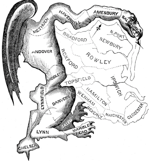
Figure 1: [37]“Gerry” and “salamander” districts, $1812$ state senate election, Massachusetts.

Gerrymandering, namely deliberate creations of district maps with highly asymmetric electoral outcomes to disenfranchise voters, has continued to be a curse to fairness of electoral systems in USA for a long time in spite of general public disdain for it. There is a long history of this type of voter disenfranchisement going back as early as $1812$ when the specific term “gerrymandering” was coined after a redistricting of the senate election map of the state of Massachusetts resulted in a South Essex district taking a shape that resembled a salamander (see Fig. 1). There is an elaborate history of litigations involving gerrymandering as well. In $1986$ the US Supreme Court (SCOTUS) ruled that gerrymandering is justiciable [10], but they could not agree on an effective way of estimating it. In $2006$, SCOTUS opined that a measure of partisan symmetry may be a helpful tool to understand and remedy gerrymandering [18], but again a precise quantification of partisan symmetry that will be acceptable to the courts was left undecided. Indeed, formulating precise and computationally efficient measures for partisan bias (i.e., lack of partisan symmetry) that will be acceptable in courts may be considered critical to removal of gerrymandering.

Although there is no dearth of legal briefs filed in courts involving gerrymandering over many years in the past, it is only more recently that mathematicians and applied computational researchers have started to investigate this topic, perhaps due to the tremendous progress in high-speed computation in the last two decades. For example, researchers in [4, 32, 31, 23, 5, 22, 16, 1, 15] have made conceptual or empirical attempts at quantifying gerrymandering and devising redistricting methods to optimize such quantifications using well-known notions such as compactness and symmetry, whereas researchers in [6, 1, 8, 19, 31, 7] have investigated designing efficient heuristic approach and other computer simulation approaches for this purpose. Two recent research directions deserve specific mentions here. In the first direction, researchers Stephanopoulos and McGhee in several papers such as [21, 30] introduced a new gerrymandering measure called the efficiency gap that attempts to minimize the absolute difference of total wasted votes between the parties in a two-party electoral system, and very importantly, at least from a legal point of view, this measure was found legally convincing in a US appeals court in a case that claims that the legislative map of the state of Wisconsin is gerrymandered. In another direction, and perhaps of considerable interest to the algorithmic game theory researchers, the authors in a recent paper [25] formulated the redistricting process as a two-person game and analyzed the performances of two kinds of protocols for such games.

1.1 Why write this article and why theoretical computer science researchers should care?

Somewhat unfortunately, even though the science of gerrymandering have received varying degrees of attention from legal researchers, mathematicians and applied computational researchers, it has received relatively little attention so far from the theoretical computer science (TCS) researchers (where by “TCS researchers” we mean researchers dealing with theoretical analysis of computational complexity issues of these problems, such as polynomial-time solvabilities, fixed-parameter tractabilities, approximability issues, etc.), except few recent results such as [6]. In our opinion there are several reasons for this. Often, some of these problems are described in “non-CS non-math” journals in a way that may not be very precise and may not be very easy for TCS researchers to follow. Another possible reason is the lack of effective collaboration between TCS researchers and other (perhaps non-CS) researchers working on these problems, perhaps accentuated by the lack of coverage of these topics in TCS publication venues. One of our goals in writing this article is to improve upon this situation. To this effect, the article is motivated by the following two high-level aims:

(I) Formalization of models and problem statements:

Our formal definitions and descriptions need to satisfy two (perhaps mutually conflicting) goals. The levels of abstraction should be as close to their real-world applications as possible but should still make the problems sufficiently interesting so as to to attract the attention of the TCS researchers.

(II) Computational complexity analysis:

We provide computational complexity analysis of some versions of these problems, leaving other versions for future research.

Task (I) may not necessarily be as straightforward as it seems, especially since descriptions of some of the problem variations may come from non-CS-theory (perhaps legal) venues. Regarding Task (II), one may wonder why computational complexity analysis (including computational hardness results) may of be practical interest at all. To this, we point out a few reasons.

1. When a particular type of gerrymandering solution is found acceptable in courts, one would eventually need to develop and implement a software for this solution, especially for large US states such as California and Texas where manual calculations may take too long or may not provide the best result. Any exact or approximation algorithms designed by TCS researchers would be a valuable asset in that respect. Conversely, appropriate computational hardness results can be used to convince a court to not apply that measure for specific US states due to practical infeasibility.

2. Beyond scientific implications, TCS research works may also be expected to have a beneficial impact on the US judicial system. Some justices, whether at the Supreme Court level or in lower courts, seem to have a reluctance to taking mathematics, statistics and computing seriously [29, 12]. TCS research may be able to help showing that the theoretical methods, whether complicated or not (depending on one’s background), can in fact yield fast accurate computational methods that can be applied to “un-gerrymander” the currently gerrymandered maps.

1.2 Remarks on the impact of the SCOTUS gerrymandering ruling

As this article was being written, SCOTUS issued a ruling on 06/27/2019 on two gerrymandering cases [28]. However, the ruling does not eliminate the need for future gerrymandering studies. While SCOTUS agreed that gerrymandering was anti-democratic, it decided that it is best settled at the legislative and political level, and it encouraged solving the problem at the state court level and delegating legislative redistricting to independent commissions via referendums. Both of the last two remedies do require further scientific studies on gerrymandering. It is also possible that a future SCOTUS may overturn this recent ruling.

2 Precise formulations of several gerrymandering problems

We assume for the rest of the paper that our political system consists of two parties only, namely Party A and Party B. This means that we ignore negligible third-party votes as is commonly done by researchers interested in two-party systems. Although some of our concepts can be extended for three or more major parties, we urge caution since gerrymandering for multi-party systems may need different definitions.

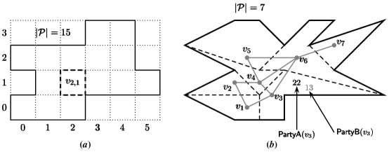
Figure 2: (a) A rectilinear polygon map $\mathcal{P}$ of size $15$ placed on a grid of size $6\times 4$; the cell $v_{2,1}$ is shown. (b) An arbitrary polygon map $\mathcal{P}$ of size $7$. The corresponding planar graph is shown in gray.

2.1 Input data and its granularity levels

The topological part of an input is generically referred to a “map” $\mathcal{P}$ which is partitioned into atomic elements or cells (e.g., subdivisions of counties or voting tabulation districts in legal gerrymandering literatures). The following two types of maps may be considered.

Rectilinear polygon $\boldsymbol{\mathcal{P}}$ without holes (Fig. 2 (a)):

For this case, $\mathcal{P}$ is placed on a unit grid of size $m\times n$. Then, the atomic elements (cells) of $\mathcal{P}$ are identified with individual unit squares of the grid inside $\mathcal{P}$. We will refer to the cell on the $i^{\rm th}$ row and $j^{\rm th}$ column by $v_{i,j}$ for $0\leq i<m$ and $0\leq j<n$.

Arbitrary polygon $\boldsymbol{\mathcal{P}}$ without holes (Fig. 2 (b)):

For this case, $\mathcal{P}$ is an arbitrary simple polygon, and the atomic elements (cells) of $\mathcal{P}$ are arbitrary sub-polygons (without holes) inside $\mathcal{P}$. Such a map can also be thought of a planar graph $G(\mathcal{P})$ whose nodes are the cells, and an edge connects two cells if they share a portion of the boundary of non-zero measure. Note that although the planar graph for a given polygonal map is unique, for a given planar graph there are many polygonal maps.

In either case, the size $|\mathcal{P}|$ of the map is the number of cells (resp., nodes) in it and, for a cell (resp., a node) $y$ and a sub-polygon $\mathcal{P}^{\prime}$ inside the polygonal map $\mathcal{P}$ (resp., a sub-graph $G^{\prime}$ of $G(\mathcal{P})$) the notation $y\in\mathcal{P}^{\prime}$ will indicate that $y$ is inside $\mathcal{P}^{\prime}$ (resp., $y$ is a node of $G^{\prime}$). Every cell or node $y$ of a map has the following numbers associated with it (see Fig. 2 (b)):

1. A strictly positive integer ${\mathsf{Pop}}(y)>0$ indicating the “total population” inside $y$.

2. Two non-negative integers ${\mathsf{PartyA}}(y),{\mathsf{PartyB}}(y)\geq 0$ such that ${\mathsf{PartyA}}(y)+{\mathsf{PartyB}}(y)={\mathsf{Pop}}(y)$. ${\mathsf{PartyA}}(y)$ and ${\mathsf{PartyB}}(y)$ denotes the total number of voters for Party A and Party B, respectively.

In addition to the above numbers, we are also given a positive integer $1<\kappa<|\mathcal{P}|$ that denotes the required (legally mandated) number of districts. Based on existing literatures, three types of granularities of these numbers in the input data can be formalized:

Course granularity:

For this case, the ${\mathsf{Pop}}(y)$’s are numbers of arbitrary size, and thus the total number of bits needed to represent the ${\mathsf{Pop}}(y)$’s (i.e., $\sum_{y}\lceil\log_{2}(1+{\mathsf{Pop}}(y))\rceil$) contributes to the size of the input. This kind of data is obtained, for example, when one uses data at the “county” level [6] or “census block group” level [9, 11].

Fine granularity:

For this case, for every cell or node $y$ we have $0<{\mathsf{Pop}}(y)\leq c$ for some fixed constant $c>0$. This kind of data is obtained, for example, when one uses data at the “Voting Tabulation District” (VTD) level or at the “census block” level.

Ultra-fine granularity:

For this case, ${\mathsf{Pop}}(y)=c$ for some fixed constant $c>0$ for every cell or node $y$. If the different ${\mathsf{Pop}}(y)$’s in the fine granularity case do not differ from each other too much then depending on the optimization objective it may be possible to approximate the fine granularity by an ultra-fine granularity.

2.2 Legal requirements for valid re-districting plans

Let $\mathcal{S}$ denote the set of all cells (resp., all nodes) in the given polygonal map $\mathcal{P}$ (resp., the planar graph $G(\mathcal{P})$). A districting scheme is a partition of $\mathcal{S}$ into $\kappa$ subsets of cells (resp., nodes), say $\mathcal{S}_{1},\dots,\mathcal{S}_{\kappa}$. One absolutely legally required condition is the following:

“every $\mathcal{S}_{j}$ must be a connected polygon (resp., a connected subgraph)”.

For convenience, we define the following quantities for each $\mathcal{S}_{j}$:

Party affiliations in $\mathcal{S}_{j}$:

${\mathsf{PartyA}}(\mathcal{S}_{j})=\sum_{y\in\mathcal{S}_{j}}{\mathsf{PartyA}}(y)$ and ${\mathsf{PartyB}}(\mathcal{S}_{j})=\sum_{y\in\mathcal{S}_{j}}{\mathsf{PartyB}}(y)$.

Population of $\mathcal{S}_{j}$:

${\mathsf{Pop}}(\mathcal{S}_{j})={\mathsf{PartyA}}(\mathcal{S}_{j})+{\mathsf{PartyB}}(\mathcal{S}_{j})$.

Then, another legally mandated condition in its two forms can be stated as follows.

Strict partitioning criteria:

Ideally, one would like $\{\mathcal{S}_{1},\dots,\mathcal{S}_{\kappa}\}$ to be a (exact) $\kappa$-equipartition of $\mathcal{S}$, i.e.,

$$\forall\,j:\,{\mathsf{Pop}}(\mathcal{S}_{j})\in\{\lfloor{\mathsf{Pop}}(\mathcal{S})/\kappa\rfloor,\,\lceil{\mathsf{Pop}}(\mathcal{S})/\kappa\rceil\}$$

Approximately strict partitioning criteria:

In practice, it is nearly impossible to satisfy the strict partitioning criteria. To alleviate this difficulty, the exactness of equipartition is relaxed by allowing ${\mathsf{Pop}}(\mathcal{S}_{1})$, $\dots$, ${\mathsf{Pop}}(\mathcal{S}_{\kappa})$ to differ from each other within an acceptable range. To this effect, we define an $\varepsilon$-approximate $\kappa$-equipartition of $\mathcal{S}$ for a given $\varepsilon>0$ to be one that satisfies $\dfrac{\max_{1\leq j\leq\kappa}\left\{{\mathsf{Pop}}(\mathcal{S}_{j})\right\}}{\min_{1\leq j\leq\kappa}\left\{{\mathsf{Pop}}(\mathcal{S}_{j})\right\}}\leq 1+\varepsilon$. Rulings such as [33] seem to suggest that the courts may allow a maximum value of $\varepsilon$ in the range of $0.05$ to $0.1$. Another possibility is to have an additive $\delta$-approximation to the strict partitioning criterion by allowing $\max_{1\leq j\leq\kappa}\left\{{\mathsf{Pop}}(\mathcal{S}_{j})\right\}\leq\min_{1\leq j\leq\kappa}\left\{{\mathsf{Pop}}(\mathcal{S}_{j})\right\}\,+\,\delta$.

2.3 Optimization objectives to eliminate partisan bias

We describe a few objective functions for optimization to remove partisan bias (in TCS frameworks) that have been proposed in existing literatures or court documents. Let $\mathcal{S}_{1},\dots,\mathcal{S}_{\kappa}$ be the set of $\kappa$ districts (partitions) of the set of all cells (resp., nodes) $\mathcal{S}$ in the given polygonal (resp., planar graph) map. We first define a few related useful notations and concepts.

Winner of a district $\mathcal{S}_{j}$:

Clearly if ${\mathsf{PartyA}}(\mathcal{S}_{j})>{\mathsf{Pop}}(\mathcal{S}_{j})/2$ then Party A should be the winner and if ${\mathsf{PartyB}}(\mathcal{S}_{j})>{\mathsf{Pop}}(\mathcal{S}_{j})/2$ then Party B should be the winner. What if ${\mathsf{PartyA}}(\mathcal{S}_{j})={\mathsf{PartyB}}(\mathcal{S}_{j})={\mathsf{Pop}}(\mathcal{S}_{j})/2$ ? Most existing research works assigned the district to a specific preferred party (e.g., Party A) always for this case, so we will assume this by default. However, in reality, a (fair) coin-toss is often used to decide the outcome.

Normalized seat counts and seat margins of the two parties:

$$\begin{array}[]{cc}\textstyle{\mbox{\sf N-Seat-C}}(\mbox{Party~{}{A}})={\big{|}\left\{\mathcal{S}_{j}\,:\,\mbox{Party~{}{A}\ wins $\mathcal{S}_{j}$}\right\}\big{|}}/{\kappa},&\textstyle\,\,{\mbox{\sf N-Seat-M}}(\mbox{Party~{}{A}})={\mbox{\sf N-Seat-C}}(\mbox{Party~{}{A}})\,-\,\nicefrac{{1}}{{2}}\\[3.0pt] \textstyle{\mbox{\sf N-Seat-C}}(\mbox{Party~{}{B}})=1\,-\,{\mbox{\sf N-Seat-C}}(\mbox{Party~{}{A}}),&\textstyle\,\,{\mbox{\sf N-Seat-M}}(\mbox{Party~{}{B}})={\mbox{\sf N-Seat-C}}(\mbox{Party~{}{B}})\,-\,\nicefrac{{1}}{{2}}\end{array}$$

Normalized vote counts and vote margins of the two parties:

$$\begin{array}[]{cc}\textstyle{\mbox{\sf N-Vote-C}}(\mbox{Party~{}{A}})={{\mathsf{PartyA}}(\mathcal{S})}/{{\mathsf{Pop}}(\mathcal{S})},&\textstyle\,\,\,\,{\mbox{\sf N-Vote-M}}(\mbox{Party~{}{A}})={\mbox{\sf N-Vote-C}}(\mbox{Party~{}{A}})-\nicefrac{{1}}{{2}},\\[3.0pt] {\mbox{\sf N-Vote-C}}(\mbox{Party~{}{B}})={{\mathsf{PartyB}}(\mathcal{S})}/{{\mathsf{Pop}}(\mathcal{S})},&\textstyle\,\,\,\,{\mbox{\sf N-Vote-M}}(\mbox{Party~{}{B}})={\mbox{\sf N-Vote-C}}(\mbox{Party~{}{B}})-\nicefrac{{1}}{{2}}\end{array}$$

Wasted votes:

For a district $\mathcal{S}_{j}$, the wasted votes (i.e., the votes whose absence would not have altered the election) for the two parties are defined as follows [30, 21]:

$${\mbox{\sf Wasted-Votes}}(\mathcal{S}_{j},\mbox{Party~{}{A}})=\left\{\begin{array}[]{r l}{\mathsf{PartyA}}(\mathcal{S}_{j})-({\mathsf{Pop}}(\mathcal{S}_{j})/2),&\mbox{if Party~{}{A}\ is the winner of $\mathcal{S}_{j}$ }\\[3.0pt] {\mathsf{PartyA}}(\mathcal{S}_{j}),&\mbox{otherwise}\end{array}\right.$$

$${\mbox{\sf Wasted-Votes}}(\mathcal{S}_{j},\mbox{Party~{}{B}})=\left\{\begin{array}[]{r l}{\mathsf{PartyB}}(\mathcal{S}_{j})-({\mathsf{Pop}}(\mathcal{S}_{j})/2),&\mbox{if Party~{}{B}\ is the winner of $\mathcal{S}_{j}$}\\[3.0pt] {\mathsf{PartyB}}(\mathcal{S}_{j}),&\mbox{otherwise}\end{array}\right.$$

Without loss of generality, assume that ${\mathsf{PartyA}}(\mathcal{S})\geq{\mathsf{PartyB}}(\mathcal{S})$. Based on the above notions, we can now describe a few optimization objectives:

Seat-vote equation:

For the decision version of this problem, we are required to produce a re-districting plan that exactly satisfies a relationship between between normalized seat counts and normalized vote counts between the two parties. The relationship was stated by [32] as

$${\mbox{\sf N-Seat-C}}(\mbox{Party~{}{A}})\,/\,{\mbox{\sf N-Seat-C}}(\mbox{Party~{}{B}})\approx\big{(}{\mathsf{PartyA}}(\mathcal{S})\,/\,{\mathsf{PartyB}}(\mathcal{S})\big{)}^{\rho}$$ (1)

where $\rho$ is a positive number and $\approx$ denotes almost equality. Kendall and Stuart in [17] argued in favor of $\rho=3$ using some stochastic models. Some special cases of Equation (1) are as follows:

Proportional representation: $\rho=1$,             Winner-take-all: $\rho=\infty$.

In practice, a value of $\rho\in[1,3]$ is considered to be a reasonable choice. For an optimization version of this problem, assuming $\boldsymbol{{\mbox{\sf N-Seat-C}}(\mbox{Party~{}{B}})>0}$ and assuming Party A has the responsibility to do the re-districting, we define an (asymptotic) $\varepsilon$-approximation ($\varepsilon\geq 1$) as a solution that satisfies

$$\textstyle\varepsilon^{-1}\lim\limits_{{\mathsf{Pop}}(\mathcal{S})\to\infty}\left(\frac{{\mathsf{PartyA}}(\mathcal{S})}{{\mathsf{PartyB}}(\mathcal{S})}\right)^{\rho}\leq\textstyle\lim\limits_{\kappa\to\infty}\left(\frac{{\mbox{\sf N-Seat-C}}\left(\mbox{Party~{}{A}}\right)}{{\mbox{\sf N-Seat-C}}\left(\mbox{Party~{}{B}}\right)}\right)\leq\varepsilon\lim\limits_{{\mathsf{Pop}}(\mathcal{S})\to\infty}\left(\frac{{\mathsf{PartyA}}(\mathcal{S})}{{\mathsf{PartyB}}(\mathcal{S})}\right)^{\rho}$$ (2)

Equation (2) is obviously ill-defined when ${\mbox{\sf N-Seat-C}}(\mbox{Party~{}{B}})=0$, which may indeed happen in practice for smaller values of $\kappa$ such as $\kappa=2$. We introduce appropriate modifications to Equation (2) to avoid this in the following manner. If ${\mbox{\sf N-Seat-C}}(\mbox{Party~{}{B}})=0$ then ${\mbox{\sf N-Seat-C}}(\mbox{Party~{}{A}})/\kappa=1$ and thus an exact version of the seat-vote equation would intuitively want ${\mathsf{PartyA}}(\mathcal{S})/{\mathsf{Pop}}(\mathcal{S})=1$ no matter what $\rho$ is. Thus, when ${\mbox{\sf N-Seat-C}}(\mbox{Party~{}{B}})=0$, we consider such a solution as an $\varepsilon$-approximation where

$$\textstyle\varepsilon=\lim_{{\mathsf{Pop}}(\mathcal{S})\to\infty}\left(\nicefrac{{{\mathsf{PartyA}}(\mathcal{S})}}{{{\mathsf{Pop}}(\mathcal{S})}}\right)^{-1}$$ (2)^′

Efficiency gap:

The goal here is to minimize the absolute difference of total wasted votes between the parties, i.e., we need to find a partition that minimizes

$$\textstyle{\mathsf{Effgap}}_{\kappa}(\mathcal{S},\mathcal{S}_{1},\dots,\mathcal{S}_{\kappa})=\left|\,\sum_{j=1}^{\kappa}\big{(}\,{\mbox{\sf Wasted-Votes}}(\mathcal{S}_{j},\mbox{Party~{}{A}})\,-\,{\mbox{\sf Wasted-Votes}}(\mathcal{S}_{j},\mbox{Party~{}{B}})\,\big{)}\,\right|$$

Partisan bias:

Partisan bias is a deviation from bipartisan symmetry that favors one party over the other. The underlying assumption in using this very popular measure is that both the parties should expect to receive the same number of seats given the same vote proportion, i.e., for example, if ${\mbox{\sf N-Vote-C}}(\mbox{Party~{}{A}})=0.7$ and the redistricting plan results in ${\mbox{\sf N-Seat-C}}(\mbox{Party~{}{A}})=0.4$ then assuming ${\mbox{\sf N-Vote-C}}(\mbox{Party~{}{A}})=1-0.7=0.3$ the same redistricting plan should result in ${\mbox{\sf N-Seat-C}}(\mbox{Party~{}{A}})=1-0.4=0.6$. However, since the precise distribution of voters when ${\mbox{\sf N-Vote-C}}(\mbox{Party~{}{A}})=0.3$ is not known, the distribution is generated artificially possibly based on some assumptions (which may not always be acceptable to court). Mathematically, a measure of partisan bias can be computed in the following manner.

1. Let $\alpha={\mbox{\sf N-Vote-C}}(\mbox{Party~{}{A}})-{\mbox{\sf N-Vote-C}}(\mbox{Party~{}{B}})$. Note that $\alpha\in[0,1]$.

2. Select $\beta_{1},\dots,\beta_{\kappa}\in[0,1]$ such that $\beta_{1}+\dots+\beta_{\kappa}=\alpha$. These choices depend upon the population shift model being used.

3. For every district $\mathcal{S}_{j}$, we create a district $\widetilde{\mathcal{S}_{j}}$ that corresponds to the same region (sub-polygon or sub-graph) but with the following parameters changes:

   $${\mathsf{PartyA}}(\widetilde{\mathcal{S}_{j}})={\mathsf{PartyA}}(\mathcal{S}_{j})\,-\,\beta_{j}{\mathsf{Pop}}(\mathcal{S}),\,\,\,\,{\mathsf{PartyB}}(\widetilde{\mathcal{S}_{j}})={\mathsf{PartyB}}(\mathcal{S}_{j})\,+\,\beta_{j}{\mathsf{Pop}}(\mathcal{S})$$

   Note that $\widetilde{\mathcal{S}_{1}},\dots,\widetilde{\mathcal{S}_{\kappa}}$ is another legally valid re-districting plan for $\mathcal{S}$ but for this new plan the normalized vote count for Party A is given by

   $$\textstyle\frac{\sum_{j=1}^{\kappa}{\mathsf{PartyA}}(\widetilde{\mathcal{S}_{j}})}{{\mathsf{Pop}}(\mathcal{S})}=\frac{\sum_{j=1}^{\kappa}\big{(}\,{\mathsf{PartyA}}(\mathcal{S}_{j})\,-\,\beta_{j}{\mathsf{Pop}}(\mathcal{S})\,\big{)}}{{\mathsf{Pop}}(\mathcal{S})}=\frac{{\mathsf{PartyA}}(\mathcal{S})\,-\,\alpha{\mathsf{Pop}}(\mathcal{S})\,\big{)}}{{\mathsf{Pop}}(\mathcal{S})}={\mbox{\sf N-Vote-C}}(\mbox{Party~{}{B}})$$

4. Recalculate the normalized seat count $\widetilde{{\mbox{\sf N-Seat-C}}}(\mbox{Party~{}{A}})$ for Party A for this new partition $\widetilde{\mathcal{S}_{1}},\dots,\widetilde{\mathcal{S}_{\kappa}}$.

5. Define the measure of bias as ${\mathsf{Bias}}_{\kappa}(\mathcal{S},\mathcal{S}_{1},\dots,\mathcal{S}_{\kappa})=\big{|}\widetilde{{\mbox{\sf N-Seat-C}}}(\mbox{Party~{}{A}})\,-\,{\mbox{\sf N-Seat-C}}(\mbox{Party~{}{A}})\big{|}$.

The goal is then to find a partition $\mathcal{S}_{1},\dots,\mathcal{S}_{\kappa}$ to minimize ${\mathsf{Bias}}_{\kappa}(\mathcal{S},\mathcal{S}_{1},\dots,\mathcal{S}_{\kappa})$.

Geometric compactness of a polygonal district $\mathcal{S}_{j}$:

The primary goal of using this measure is to ensure that polygonal districts do not have “unusually weird” shapes (cf. Fig. 1). A most commonly used compactness measure is the so-called “Polsby-Popper compactness measure” [27] given by $\mathscr{C}(\mathcal{S}_{j})=c\,A/B^{2}$ where $A$ is the area and $B$ is the length of the perimeter of $\mathcal{S}_{j}$, and $c>0$ is a suitable constant ($c=4\pi$ was used in [24]). The computational problem is then to find a re-districting plan such that $L_{1}\leq\mathscr{C}(\mathcal{S}_{j})\leq L_{2}$ for all $j$ for two given bounds $L_{1}$ and $L_{2}$.

In addition to what is discussed above, there are other constraints and optimization criteria, such as responsiveness (also called swing ratio), equal vote weight and declination, that we did not discuss; the reader is referred to references such as [34, 20, 3] for informal discussions on them.

2.4 Prior relevant computational complexity research

To our knowledge, the most relevant prior non-trivial computational complexity (i.e., approximation hardness, approximation algorithms, etc.) article regarding gerrymandering is [6]. The article [6] exclusively dealt with the efficiency gap measure, and provided some non-trivial approximation hardness and approximation algorithms in addition to designing and implementing a practical algorithm for this case which works well on real maps. In the terminologies of this article, [6] showed that minimization of the efficiency gap measure for rectilinear polygonal maps with coarse grain inputs and strict partitioning criteria does not admit any non-trivial polynomial-time approximation in the worst case, but does admit polynomial-time approximation algorithms when further constraints are added to the problem. In addition, [6] and [30, p. 853] also observed that $\mathsf{Effgap}_{\kappa}(\mathcal{S},\mathcal{S}_{1},\dots,\mathcal{S}_{\kappa})/{\mathsf{Pop}}(\mathcal{S})=|\,2\,\times\,{\mbox{\sf N-Vote-M}}(\mbox{Party~{}{A}})\,-\,{\mbox{\sf N-Seat-M}}(\mbox{Party~{}{A}})\,|$.

3 Our computational complexity results

Before stating our technical results, we remind the reader about the following obvious but important observations. Consider the following combinations for a pair $(X,Y)$:

1. $X$ is rectilinear polygonal input and $Y$ is arbitrary polygonal input (equivalently, a planar graph), or

2. $X$ is fine or ultra-fine granular input and $Y$ is coarse input, or

Then, the following statements hold:

1. Any computational hardness result for $X$ also implies the same result for $Y$.

2. Any approximation or exact algorithmic result for $Y$ also implies the same result for $X$.

In the statements of our theorems or lemmas, we will use the following convention. $\kappa>1$ will denote the number of districts. For polygonal maps (resp., planar graph maps) $\mathcal{S}$ ((resp., $G=(V,E)$) will denote the polygon as a collection of all cells (resp., the graph), and $\mathcal{S}_{1},\dots,\mathcal{S}_{\kappa}\subset\mathcal{S}$ ((resp., $V_{1},\dots,V_{\kappa}\subset V$) will denote an arbitrary valid (not necessarily optimal) solution. Since every state of USA has a valid current districting partition (sometimes subject to litigation), we assume that our problem has already at least one valid (but not necessarily optimal) solution that can be found in polynomial time (thus, for example, for our computational hardness results we are required to exhibit a polynomial-time valid solution).

In the following two sub-sections, we state our two computational complexity results and some relevant discussions on them, leaving the actual proofs later in Sections 4–6.

3.1 Rectilinear polygonal course granularity input

Theorem 1 (Hardness of seat-vote equation computation).

Let $\rho>0,\varepsilon\geq 1$ be two arbitrary finite rational numbers, and $c>1,\delta>0$ be any two constants arbitrarily close to $1$ and $0$, respectively. Suppose that we are allowed a (reasonably loose) additive $|\mathcal{S}|^{c}$-approximate strict partitioning criteria (i.e., the partitioning satisfies $\textstyle\max_{1\leq j\leq\kappa}\left\{{\mathsf{Pop}}(\mathcal{S}_{j})\right\}\leq\min_{1\leq j\leq\kappa}\left\{{\mathsf{Pop}}(\mathcal{S}_{j})\right\}+|\mathcal{S}|^{c}$).

(a) (Hardness when ${\mbox{\sf N-Vote-C}}(\mbox{Party~{}{A}})<\nicefrac{{1}}{{2}}$). It is $\mathsf{NP}$-hard to compute an $\varepsilon$-approximation of the seat-vote-equation optimization problem.

(b) (Hardness when ${\mbox{\sf N-Vote-C}}(\mbox{Party~{}{A}})\geq\nicefrac{{1}}{{2}}$). Let $\kappa=3\,\alpha+r$ for some two integers $\alpha\geq 1$ and $r\in\{-1,0,1\}$. Then, it is $\mathsf{NP}$-hard to distinguish between the following two cases:

1. if the seat-vote-equation has an $(\varepsilon_{\mathrm{low}}-\delta)$-approximation where $\varepsilon_{\mathrm{low}}\leq\left\{\begin{array}[]{r l}2,&\mbox{if $\kappa\in\{2,3\}$}\\ \frac{\kappa}{\alpha+1}-1,&\mbox{otherwise}\end{array}\right.$

2. or, if the seat-vote-equation has an $(\varepsilon_{\mathrm{high}}+\delta)$-approximation where $\varepsilon_{\mathrm{high}}\geq\kappa-1$.

Moreover, a valid solution that is a $(\kappa-1)$-approximation always exists irrespective of what definition of of an approximately strict partitioning criterion is used.

Remark 1.

The hardness result in (b) is tight if $\kappa=2$ since a we have a $2$-approximation. For $\kappa>2$ there is a factor gap between the two bounds that may be worthy of further investigation. Note that $\lim_{\kappa\to\infty}\varepsilon_{\mathrm{low}}=2$.

Chatterjee et al. [6] showed that the efficiency gap computation does not admit any non-trivial approximation at all using the strict partitioning criterion if the input is given at rectilinear polygonal course granularity level. The following theorem shows that the same result holds even if the strict partitioning criteria is relaxed arbitrarily.

Theorem 2 (Hardness of efficiency gap computation).

Let $\delta\geq 0,\varepsilon\geq 1$ be any two numbers. Then, it is $\mathsf{NP}$-hard to compute an $\varepsilon$-approximation of $\mathsf{Effgap}_{\kappa}(\mathcal{S},\mathcal{S}_{1},\dots,\mathcal{S}_{\kappa})$ even when we are allowed to use $\delta$-approximate $\kappa$-equipartition of $\mathcal{S}$.

3.2 Arbitrary polygonal fine granularity input

For this case, it is clearer to present our proofs if we assume that the planar graph format of our input, i.e., our input is planar graph whose nodes are the cells, and whose edges connect pairs of cells if they share a portion of the boundary of non-zero measure.

Chatterjee et al. [6] left open the complexity of the efficiency gap computation at the fine granularity level of inputs using either exact or approximate partitioning criteria. Here we show that computing the efficiency gap is $\mathsf{NP}$-complete for arbitrary polygonal fine granularity input even under approximately strict partitioning criteria.

Theorem 3 (Hardness of efficiency gap computation).

Computing $\mathsf{Effgap}_{\kappa}(\mathcal{S},\mathcal{S}_{1},\dots,\mathcal{S}_{\kappa})$ is $\mathsf{NP}$-complete even when we are allowed to use $\varepsilon$-approximate $\kappa$-equipartition of $\mathcal{S}$ for any constant $0<\varepsilon<\nicefrac{{1}}{{2}}$.

Remark 2.

The $\mathsf{NP}$-hardness reduction in Theorem 3 does not provide any non-trivial inapproximability ratio. In fact, for the specific hard instances of the gerrymandering problem constructed in the proof of Theorem 3, it is possible to design a polynomial-time approximation scheme (PTAS) for the efficiency gap computation using the approach in [2] $($the proof of such a PTAS is relatively straightforward and therefore we do not provide an explicit proof$)$.

3.3 What do results and proofs in Theorem 1 and Theorem 3 imply in the context of gerrymandering in US?

Our results are computational hardness result, so one obvious question is about the implications of these results and associated proofs for gerrymandering in US. To this effect, we offer the following motivations and insights that might be of independent interest.

On following the seat-vote equation:

Theorem 1 indicates that efficient computation of even a modest approximation to the seat-vote equation may be difficult. Thus, unless further research works indicate otherwise, it may not be a good idea to closely follow the seat-vote equation for computationally efficient elimination of gerrymandering (fortunately, many courts also do not recommend on following the seat-vote proportion too closely, though not for computational complexity reasons).

On relaxing the exact equipartition criteria:

Relaxing the exact equipartition criteria even beyond the
$\thicksim\!\!10$% margin that has traditionally been allowed by courts does not seem to make removal of gerrymandering computationally any easier.

On accurate census data at the fine granularity level:

Accurate census data at the fine granularity level may make a difference to an independent commission seeking fair districts (such as in California). As stated in Remark 2, while it is difficult to even approximately optimize the absolute difference of the wasted votes at a course granularity level of inputs, the situation at the fine granularity level of inputs may be not so hopeless.

On cracking and packing, how far one can push?

It is well-known that cracking and packing may result in large partisan bias. For example, based on $2012$ election data for election of the (federal) house of representatives for the states of Virginia, the Democratic party had a normalized vote count of about $52$% but due to cracking/packing held only $4$ of the $11$ house seats [35, 36]. This observation, coupled with the knowledge that Virginia is one of the most gerrymandered states in US both on the congressional and state levels [38], leads to the following natural question: “could the Virginia lawmakers have disadvantaged the Democratic party more by even more careful execution of cracking and packing approaches”? As one lawmaker put it quite bluntly, they would have liked to gerrymander more if only they could.

We believe a partial answer to this is provided by the proof structures for Theorems 2 and 3. A careful inspection of the proofs of Theorems 2 and  3 reveal that they do use cracking and packing to create hard instances of the efficiency gap minimization problem that are computationally intractable to solve optimally certainly at the course granularity input level and even at the fine granularity input level. Perhaps the computational complexity issues did save the Democratic party from further electoral disadvantages.

4 Proof of Theorem 1

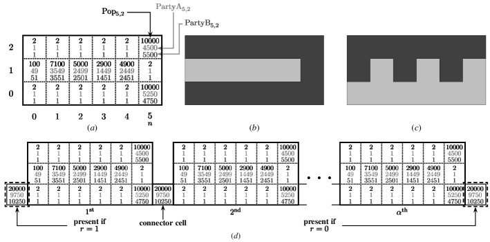
Figure 3: (a) An illustration of the construction in the proof of Theorem 1 for $\kappa=2$ when the instance of the PARTITION problem is $\mathcal{A}=\{100,7100,5000,2900,4900\}$ (and thus $W=20000$). (b) An optimal solution of the redistricting problem when a solution of the PARTITION problem exists. (c) A trivial valid solution which is not optimal. (d) Generalization of the reduction for arbitrary $\kappa\geq 2$.

(a) We reduce from the $\mathsf{NP}$-complete PARTITION problem [13] which is defined as follows:

given a set of $n$ positive integers $\mathcal{A}=\left\{a_{0},\dots,a_{n-1}\right\}$, decide if there exists a subset $\mathcal{A}^{\prime}\subset\mathcal{A}$ such that $\sum\limits_{a_{i}\in\mathcal{A}^{\prime}}a_{i}=\sum\limits_{a_{j}\notin\mathcal{A}^{\prime}}a_{j}=\frac{W}{2}$ where $W=\sum\limits_{j=0}^{n-1}a_{j}$ is an even number.

Note that we can assume without loss of generality that $n$ is sufficiently large, $n$ and each of $a_{0},\dots,a_{n-1}$ is a multiple of any fixed positive integer (in particular, multiple of $2$), $\max_{j}\{a_{j}\}<W/2$, no two integers in $\mathcal{A}$ are equal and $W>n^{2c}$.

Proof for $\kappa=2$.

Multiplying $a_{0},\dots,a_{n-1}$ and $W$ by $n^{2+2c}$, and denoting them by the same notations we can therefore assume that the minimum absolute difference between any two distinct numbers in $\mathcal{A}$ is at least $n^{2+2c}$ and $W>n^{2+4c}$. Our rectilinear polygon is a rectangle $\mathcal{S}=\left\{p_{i,j}\,|\,0\leq i\leq n,\,0\leq j\leq 2\right\}$ of size $3\times(n+1)$ (see Fig. 3 (a)) with the following numbers for various cells:

$${\mathsf{Pop}}_{i,j}=\left\{\begin{array}[]{r l}a_{i},&\mbox{if $0\leq i<n$ and $j=1$}\\ \nicefrac{{W}}{{2}},&\mbox{if $i=n,j=0$,}\\ &\,\,\,\,\mbox{or if $i=n,j=2$}\\ 2,&\mbox{otherwise}\end{array}\right.\,\,\,\,\,\,\,\,\,\,{\mathsf{PartyA}}_{i,j}=\left\{\begin{array}[]{r l}({a_{i}}/{2})-1,&\mbox{if $0\leq i<n$ and $j=1$}\\ (\nicefrac{{W}}{{4}})+50\,n,&\mbox{if $i=n,j=0$}\\ (\nicefrac{{W}}{{4}})-100\,n,&\mbox{if $i=n,j=2$}\\ 1,&\mbox{otherwise}\end{array}\right.$$

Note that:

1. ${\mathsf{Pop}}(\mathcal{S})=2\times(W/2)+\sum_{j=0}^{n-1}a_{j}+2\times(2n+1)-2=2W+4n$.

2. ${\mathsf{PartyA}}(\mathcal{S})=2\times(\nicefrac{{W}}{{4}})+50\,n-100\,n+\sum_{j=0}^{n-1}((a_{j}/2)-1)+(2n+1)=W-47n-1$.

3. ${\mbox{\sf N-Vote-C}}(\mbox{Party~{}{A}})=(W-47n-1)/(2W+4n)<\nicefrac{{1}}{{2}}$.

First, as required, we show that $\mathcal{S}$ has a valid solution satisfying all the constraints. Consider the following solution (refer to Fig. 3 (b)):

$$\mathcal{S}_{1}=\left\{p_{i,1}\,|\,a_{i}\in\mathcal{A}\right\},\,\,\,\,\,\,\mathcal{S}_{2}=\mathcal{C}\setminus\mathcal{S}_{1}$$

We can now verify the following:

$${\mathsf{Pop}}(\mathcal{S}_{1})=\sum_{a_{i}\in\mathcal{A}}a_{i}=W,\,\,\,{\mathsf{Pop}}(\mathcal{S}_{2})={\mathsf{Pop}}(\mathcal{S})-{\mathsf{Pop}}(\mathcal{S}_{1})=W+4n,$$

and thus the partitioning constraint is satisfied since $4n<(3n+3)^{c}$. Since $\lim\limits_{{\mathsf{Pop}}(\mathcal{S})\to\infty}\left(\frac{{\mathsf{PartyA}}(\mathcal{S})}{{\mathsf{PartyB}}(\mathcal{S})}\right)=1$, the proof is complete once the following claims are shown.

(completeness)

If the PARTITION problem has a solution then ${\mbox{\sf N-Seat-C}}(\mbox{Party~{}{A}})=1$.

     (soundness)

If the PARTITION problem does not have a solution then ${\mbox{\sf N-Seat-C}}(\mbox{Party~{}{A}})=0$.

Proof of completeness (refer to Fig. 3 (c))

Suppose that there is a valid solution of $\mathcal{A}^{\prime}\subset\mathcal{A}$ of PARTITION and consider the two polygons

$$\mathcal{S}_{1}=\left\{p_{i,0}\,|\,0\leq i\leq n\right\}\cup\left\{p_{i,1}\,|\,a_{i}\in\mathcal{A}^{\prime}\right\}\cup\left\{p_{n,1}\right\},\,\,\,\,\,\,\mathcal{S}_{2}=\mathcal{C}\setminus\mathcal{S}_{1}$$

One can now verify the following:

1. ${\mathsf{Pop}}(\mathcal{S}_{1})=2(n+1)+\left(\sum_{a_{i}\in\mathcal{A}^{\prime}}a_{i}\right)+\frac{W}{2}=W+2n+2$, ${\mathsf{Pop}}(\mathcal{S}_{2})={\mathsf{Pop}}(\mathcal{S})-{\mathsf{Pop}}(\mathcal{S}_{1})=W+2n-2$, and thus the partitioning constraint is satisfied since ${\mathsf{Pop}}(\mathcal{S}_{1})-{\mathsf{Pop}}(\mathcal{S}_{2})=4<(3n+3)^{c}$.

2. ${\mathsf{PartyA}}(\mathcal{S}_{1})=(n+1)+\sum_{a_{i}\in\mathcal{A}^{\prime}}\left(\frac{a_{i}}{2}-1\right)+\frac{W}{4}+50n=\frac{W}{2}+(51n+1)-|\mathcal{A}^{\prime}|$, ${\mathsf{PartyB}}(\mathcal{S}_{1})={\mathsf{Pop}}(\mathcal{S}_{1})-{\mathsf{PartyA}}(\mathcal{S}_{1})=\frac{W}{2}-49n+1+|\mathcal{A}^{\prime}|$, and thus ${\mathsf{PartyA}}(\mathcal{S}_{1})>{\mathsf{PartyB}}(\mathcal{S}_{1})$ since $|\mathcal{A}^{\prime}|<n-1$.

3. ${\mathsf{PartyA}}(\mathcal{S}_{2})={\mathsf{PartyA}}(\mathcal{S})-{\mathsf{PartyA}}(\mathcal{S}_{1})=\frac{W}{2}-98n-2+|\mathcal{A}^{\prime}|$, ${\mathsf{PartyB}}(\mathcal{S}_{2})={\mathsf{Pop}}(\mathcal{S}_{2})-{\mathsf{PartyA}}(\mathcal{S}_{2})=\frac{W}{2}+100n-|\mathcal{A}^{\prime}|$, and thus ${\mathsf{PartyA}}(\mathcal{S}_{2})<{\mathsf{PartyB}}(\mathcal{S}_{2})$ since $|\mathcal{A}^{\prime}|<n-1$.

Proof of soundness

Let $\mathcal{S}_{1}$ and $\mathcal{S}_{2}=\mathcal{S}\setminus\mathcal{S}_{1}$ be the two partitions in any valid solution of the redistricting problem. For convenience, let us define the following sets:

$$\mathcal{S}_{\mathcal{S}_{1}}=\left\{\,p_{i,1}\,|\,0\leq i<n\right\}\,\cap\,\mathcal{S}_{1},\,\,\,\,\mathcal{S}_{\mathcal{S}_{2}}=\left\{\,p_{i,1}\,|\,0\leq i<n\right\}\,\cap\,\mathcal{S}_{2}$$

$$\mathcal{S}_{heavy}=\left\{p_{n,0},p_{n,2}\right\},\,\,\,\,\mathcal{S}_{light}=\mathcal{S}\setminus\left(\mathcal{S}_{heavy}\,\cup\,\mathcal{S}_{\mathcal{S}_{1}}\,\cup\,\mathcal{S}_{\mathcal{S}_{2}}\right)$$

The following chain of arguments prove the desired claim.

(i)

Both the cells in $\mathcal{S}_{heavy}$ cannot be together in the same partition, say $\mathcal{S}_{1}$, with any cell, say $p_{i,1}$, from $\mathcal{S}_{\mathcal{S}_{1}}\cup\mathcal{S}_{\mathcal{S}_{2}}$ since in that case

$${\mathsf{Pop}}(\mathcal{S}_{1})\geq W+a_{i}\,\,\,\&\,\,\,{\mathsf{Pop}}(\mathcal{S}_{2})={\mathsf{Pop}}(\mathcal{S})-{\mathsf{Pop}}(\mathcal{S}_{1})\leq W+4n-a_{i}\\ \Rightarrow\,{\mathsf{Pop}}(\mathcal{S}_{1})-{\mathsf{Pop}}(\mathcal{S}_{2})\geq 2a_{i}-4n>2\,n^{2+2c}-4n>n^{2+2c}>|\mathcal{S}|^{c}=(3n+3)^{c}$$

(ii)

At least one of $\mathcal{S}_{\mathcal{S}_{1}}$ and $\mathcal{S}_{\mathcal{S}_{2}}$ must be empty. To see this, assume that both are non-empty. By (i), we may suppose that $p_{n,0}\in\mathcal{S}_{1}$ and $p_{n,2}\in\mathcal{S}_{1}$. Since the PARTITION problem does not have a solution, $L=\sum\limits_{p_{i,1}\in\mathcal{S}_{\mathcal{S}_{1}}}a_{i}\neq M=\sum\limits_{p_{i,1}\in\mathcal{S}_{\mathcal{S}_{2}}}a_{i}$. Assume, without loss of generality, that $L>M$. Then, $L-M\geq\min\limits_{0\leq i<n}\{a_{i}\}\geq n^{2+2c}$, and therefore $|\,{\mathsf{Pop}}(\mathcal{S}_{1})-{\mathsf{Pop}}(\mathcal{S}_{2})\,|\geq|\,(L-M)-{\mathsf{Pop}}(\mathcal{S}_{light})\,|>n^{1+2c}>|\mathcal{S}|^{c}$, thus violating the partitioning constraints.

(iii)

Since both $\mathcal{S}_{\mathcal{S}_{1}}$ and $\mathcal{S}_{\mathcal{S}_{2}}$ cannot be empty, by (ii) assume that $\mathcal{S}_{\mathcal{S}_{1}}=\emptyset$ but $\mathcal{S}_{\mathcal{S}_{2}}\neq\emptyset$. Then, by (i), both $p_{n,0}$ and $p_{n,2}$ are in $\mathcal{S}_{1}$. We can now verify that ${\mbox{\sf N-Seat-C}}(\mbox{Party~{}{A}})=0$ as follows:

• ${\mathsf{PartyA}}(\mathcal{S}_{1})\leq\frac{W}{4}+50n+\frac{W}{4}-100n+2n+1=\frac{W}{2}-48n+1$, ${\mathsf{PartyB}}(\mathcal{S}_{2})\geq\frac{W}{4}-50n+\frac{W}{4}+100n=\frac{W}{2}+50n$, and thus ${\mathsf{PartyA}}(\mathcal{S}_{1})<{\mathsf{PartyB}}(\mathcal{S}_{1})$.

• ${\mathsf{PartyA}}(\mathcal{S}_{2})\leq\sum_{j=0}^{n-1}\left(\frac{a_{j}}{2}-1\right)+n=\frac{W}{4}$, ${\mathsf{PartyB}}(\mathcal{S}_{2})\geq\sum_{j=0}^{n-1}\left(\frac{a_{j}}{2}+1\right)\frac{W}{4}+n$, and thus ${\mathsf{PartyA}}(\mathcal{S}_{1})<{\mathsf{PartyB}}(\mathcal{S}_{1})$.

Proof for $\kappa\geq 2$.

Let $\kappa=3\,\alpha+r$ for some two integers $\alpha\geq 1$ and $r\in\{-1,0,1\}$. For this case, we will use $\alpha$ copies, say $\mathcal{S}^{(1)},\mathcal{S}^{(2)},\dots,\mathcal{S}^{(\alpha)}$, of the $3\times(n+1)$ rectangle $\mathcal{S}$ used for the previous case connected via $\alpha-1$ connector cells, say $\mathcal{C}^{(1)},\mathcal{C}^{(2)},\dots,\mathcal{C}^{(\alpha-1)}$, plus additional one or two cells, say $\mathcal{C}^{(\alpha)}$ and $\mathcal{C}^{(\alpha+1)}$, depending on whether the value of $r$ is $0$ or $1$, respectively (refer to Fig. 3 (d)). We now multiply $a_{0},\dots,a_{n-1}$ and $W$ by $n^{3+2c}\kappa^{2}$, and again denoting them by the same notations we can therefore assume that the minimum absolute difference between any two distinct numbers in $\mathcal{A}$ is at least $n^{3+2c}\kappa^{2}$ and $W>n^{3+4c}\kappa^{2}$. We assign the required numbers to the connector and additional cells as follows: ${\mathsf{Pop}}(\mathcal{C}^{(j)})=W$ and ${\mathsf{PartyA}}(\mathcal{C}^{(j)})=\frac{W}{2}-50n$ for all $j$. Letting $\beta=\alpha+r$ denote the actual number of connector cells, we now have the following updated calculations:

$${\mathsf{Pop}}(\mathcal{S})=\alpha(2W+4n)+\beta W,\,\,\,{\mathsf{PartyA}}(\mathcal{S})=\alpha(W-47n-1)+\beta\left(\frac{W}{2}-50n\right)$$

$$|\mathcal{S}|=3\,\alpha\,(n+1)+(\alpha+r)=3\,\alpha\,n+4\,\alpha+r\leq(\kappa+1)n+\frac{4\kappa}{3}+\frac{7}{3}<2\,\kappa\,n$$

$${\mbox{\sf N-Vote-C}}(\mbox{Party~{}{A}})=\frac{{\mathsf{PartyA}}(\mathcal{S})}{{\mathsf{Pop}}(\mathcal{S})}<\nicefrac{{1}}{{2}},\,\,\,\text{as required}$$

Claim 1.

Any of the connector or additional cells cannot appear in the same partition with a cell from $\mathcal{S}^{(j)}_{heavy}=\left\{p_{jn+(j-1)+r,0},p_{jn+(j-1)+r,2}\right\}$ for any $j$.

Proof.  Suppose that the connector cell $\mathcal{C}^{(i)}$ is together with at least one of two cells from $\mathcal{S}^{(j)}_{heavy}$ in a partition, say $\mathcal{S}_{p}$. Then, ${\mathsf{Pop}}(\mathcal{S}_{p})=\frac{W}{2}+W=\frac{3W}{2}$. Note that

$$\frac{{\mathsf{Pop}}(\mathcal{S})}{\kappa}=\frac{\alpha(2W+4n)+\beta W}{\kappa}=\frac{(2\alpha+\beta)W+4\alpha n}{\kappa}=\frac{(3\alpha+r)W+4\alpha n}{\kappa}\\ =\frac{\kappa W+4\alpha n}{\kappa}W+\frac{4n}{3}\times\frac{\kappa-r}{\kappa}<W+\frac{5n}{3}$$

and thus there exists a partition $\mathcal{S}_{q}$, $q\neq p$, such that ${\mathsf{Pop}}(\mathcal{S}_{q})<W+\frac{5n}{3}$. Consequently, it follows that

$${\mathsf{Pop}}(\mathcal{S}_{p})-{\mathsf{Pop}}(\mathcal{S}_{q})>\frac{3W}{2}-W+\frac{5n}{3}>\frac{4W}{3}>\frac{4}{3}n^{3+4c}\kappa^{2}>|\mathcal{S}|^{c}$$

which violates the partitioning constraint. ❑

It is possible to generalize the proof for $\kappa=2$ to $\kappa>2$. Intuitively, if there is a solution to the PARTITION problem then one of the two seats in each copy $\mathcal{S}^{(j)}$ is won by Party A but otherwise Party A wins no seat at all. The correspondingly modified completeness and soundness claims are as follows:

(completeness for $\kappa>2$)

If the PARTITION problem has a solution then ${\mbox{\sf N-Seat-C}}(\mbox{Party~{}{A}})=\alpha$.

(soundness for $\kappa>2$)

If the PARTITION problem does not have a solution then ${\mbox{\sf N-Seat-C}}(\mbox{Party~{}{A}})=0$.

(b) We can use a proof similar to that in (a) for $\kappa\geq 2$, but we need to change some of the numbers. More precisely, the cell $p_{n+r,0}\in\mathcal{S}^{(1)}_{heavy}$ in the very first copy $\mathcal{S}^{(1)}$ has the following new number (instead of the previous value of $(W/4)-100\,n$) corresponding to the total number of voters for Party A: ${\mathsf{PartyA}}(p_{n+r,0})=(W/4)+q\,\alpha^{2}n^{2}$ where $q\geq 0$ is the smallest integer such that $q\alpha^{2}n^{2}+100n-49\alpha n-\alpha-50n\beta\geq 0$. Note that ${\mathsf{PartyB}}(p_{n+r,0})=(W/2)-{\mathsf{PartyA}}(p_{n+r,0})>0$ since $W>n^{3+4c}\kappa^{2}$. A relevant calculation is:

$${\mathsf{PartyA}}(\mathcal{S})-\frac{{\mathsf{Pop}}(\mathcal{S})}{2}=\left[\alpha(W-47n-1)+100n+q\alpha^{2}n^{2}+\beta\left(\frac{W}{2}-50n\right)\right]-\left[\alpha(W+2n)+\beta\frac{W}{2}\right]\\ =q\alpha^{2}n^{2}+100n-49\alpha n-\alpha-50n\beta\geq 0$$

and therefore ${\mbox{\sf N-Vote-C}}(\mbox{Party~{}{A}})=\frac{{\mathsf{PartyA}}(\mathcal{S})}{{\mathsf{Pop}}(\mathcal{S})}\geq\nicefrac{{1}}{{2}}$, as required. The only difference in the proofs come from the fact that now in the first copy $\mathcal{S}^{(1)}$ Party A always wine one seat by default but wins two seats if PARTITION has a solution. The correspondingly modified completeness and soundness claims are as follows:

(modified completeness claim for ${\mbox{\sf N-Vote-C}}(\mbox{Party~{}{A}})>\nicefrac{{1}}{{2}}$)

If the PARTITION problem has a solution then ${\mbox{\sf N-Seat-C}}(\mbox{Party~{}{A}})=\alpha+1$.

(modified soundness claim for ${\mbox{\sf N-Vote-C}}(\mbox{Party~{}{A}})>\nicefrac{{1}}{{2}}$)

If the PARTITION problem does not have a solution then ${\mbox{\sf N-Seat-C}}(\mbox{Party~{}{A}})=1$.

To see that these completeness and soundness claims indeed prove the desired bounds, note the following:

1. $a=\lim\limits_{{\mathsf{Pop}}(\mathcal{S})\to\infty}\left(\frac{{\mathsf{PartyA}}(\mathcal{S})}{{\mathsf{PartyB}}(\mathcal{S})}\right)=1$ and $b=\lim\limits_{{\mathsf{Pop}}(\mathcal{S})\to\infty}\left(\frac{{\mathsf{PartyA}}(\mathcal{S})}{{\mathsf{Pop}}(\mathcal{S})}\right)=\nicefrac{{1}}{{2}}$.

2. If $\kappa=2$ and ${\mbox{\sf N-Seat-C}}(\mbox{Party~{}{A}})=\alpha+1=2$, then ${\mbox{\sf N-Seat-C}}(\mbox{Party~{}{B}})=0$, and thus this gives a $2$-approximation since $1/b=2$.

3. If $\kappa=3$ and ${\mbox{\sf N-Seat-C}}(\mbox{Party~{}{A}})=\alpha+1=2$, then ${\mbox{\sf N-Seat-C}}(\mbox{Party~{}{B}})=1$, and thus this gives a $2$-approximation since $\frac{{\mbox{\sf N-Seat-C}}(\mbox{Party~{}{A}})}{{\mbox{\sf N-Seat-C}}(\mbox{Party~{}{B}})}=2$.

4. For any $\kappa\geq 2$, if ${\mbox{\sf N-Seat-C}}(\mbox{Party~{}{A}})=1$ then ${\mbox{\sf N-Seat-C}}(\mbox{Party~{}{B}})=\kappa-1$ and thus this gives a $(\kappa-1)$-approximation.

For the existence of a $\kappa$-approximation when ${\mbox{\sf N-Vote-C}}(\mbox{Party~{}{A}})\geq\nicefrac{{1}}{{2}}$, note that for any valid solution $\mathcal{S}_{1},\dots,\mathcal{S}_{\kappa}$ for $\mathcal{S}$, ${\mbox{\sf N-Vote-C}}(\mbox{Party~{}{A}})=\dfrac{{\mathsf{PartyA}}(\mathcal{S})}{{\mathsf{Pop}}(\mathcal{S})}=\dfrac{\sum_{i=1}^{\kappa}{\mathsf{PartyA}}(\mathcal{S}_{i})}{\sum_{i=1}^{\kappa}{\mathsf{Pop}}(\mathcal{S}_{i})}\geq\nicefrac{{1}}{{2}}$, and thus there must exists a district $\mathcal{S}_{j}$ such that ${\mathsf{PartyA}}(\mathcal{S}_{j})\geq\nicefrac{{{\mathsf{Pop}}(\mathcal{S}_{j})}}{{2}}$.

5 Proof sketch of Theorem 2

The proof is obtained by carefully modifying the proof of Theorem 4 in [6] in the following manner:

1. We remove all cells with zero population. As a result, the rectangle in [6] now becomes a rectilinear polygon (without holes).

2. We multiply all the non-zero values of ${\mathsf{Pop}}(\cdot)$’s and ${\mathsf{PartyA}}(\cdot)$’s by $1+2\delta$. It is possible to verify that as a result the following claim holds:

   for any two districts $\mathcal{S}_{i}$ and $\mathcal{S}_{j}$, ${\mathsf{Pop}}(\mathcal{S}_{i})\neq{\mathsf{Pop}}(\mathcal{S}_{j})$ implies either ${\mathsf{Pop}}(\mathcal{S}_{i})>(1+\varepsilon){\mathsf{Pop}}(\mathcal{S}_{j})$ or ${\mathsf{Pop}}(\mathcal{S}_{j})>(1+\varepsilon){\mathsf{Pop}}(\mathcal{S}_{i})$.

   This ensures that ${\mathsf{Pop}}(\mathcal{S}_{1})=\dots={\mathsf{Pop}}(\mathcal{S}_{\kappa})$ for any valid partition of the rectilinear polygon.

3. The new soundness and completeness claims now become as follows:

   (soundness)

   If the PARTITION problem does not have a solution then $\mathsf{Effgap}_{\kappa}(\mathcal{S},\mathcal{S}_{1},\dots,\mathcal{S}_{\kappa})=\delta\Delta$.

   (completeness)

   If the PARTITION problem has a solution then $\mathsf{Effgap}_{\kappa}(\mathcal{S},\mathcal{S}_{1},\dots,\mathcal{S}_{\kappa})=0$.

   where $\Delta$ is exactly as defined in [6]

6 Proof of Theorem 3

The problem is trivially in $\mathsf{NP}$, so will concentrate on the $\mathsf{NP}$-hardness reduction. Our reduction is from the maximum independent set problem for planar cubic graphs (Mis_PC) which is defined as follows:

“given a cubic (i.e., $3$-regular) planar graph $G=(V,E)$ and an integer $\nu$, does there exist an independent set for $G$ with $\nu$ nodes ?”

Mis_PC is known to be $\mathsf{NP}$-complete [14] but there exists a PTAS for it [2]. Note the value of
$\mathsf{Effgap}_{\kappa}(\mathcal{S},\mathcal{S}_{1},\dots,\mathcal{S}_{\kappa})$ remains the same if we divide (or multiply) the values of all ${\mathsf{PartyA}}(\mathcal{S}_{j})$’s and ${\mathsf{PartyB}}(\mathcal{S}_{j})$’s by $t$ for any integer $t>0$. Thus, to simplify notation, we assume that we have re-scaled the numbers such that $\min_{1\leq j\leq\kappa}\left\{{\mathsf{Pop}}(\mathcal{S}_{j})\right\}=1$ and therefore our approximately strict partitioning criteria is satisfied by ensuring that $1\leq{\mathsf{Pop}}(\mathcal{S}_{j})\leq 1+\varepsilon$ for all $j=1,\dots,\kappa$ with ${\mathsf{Pop}}(\mathcal{S}_{j})=1$ for at least one $j$. Thus, each ${\mathsf{PartyA}}(\mathcal{S}_{j})$, ${\mathsf{PartyB}}(\mathcal{S}_{j})$ and ${\mathsf{Pop}}(\mathcal{S}_{j})$ may be positive rational constant numbers such that, if needed, we can ensure that all these numbers are integers at the end of the reduction by multiplying them by a suitable positive integer of polynomial size.

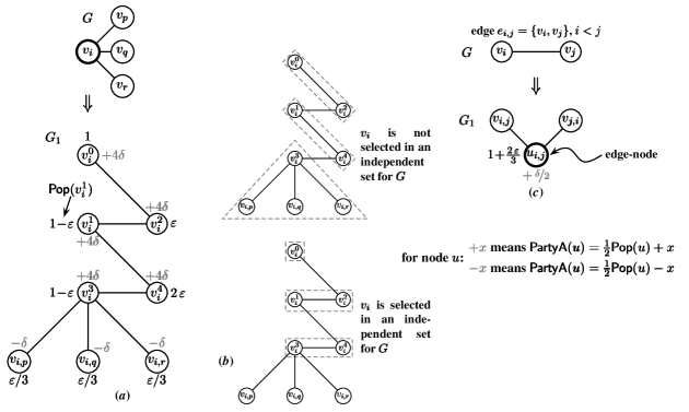
Figure 4: The sub-graph gadgets used in the proof of Theorem 3.

Let $G=(V,E)$ and $\nu$ be the given instance of Mis_PC with $V=\{v_{1},\dots,v_{n}\}$ and $|E|=3n/2$. Note that, since $G$ is cubic, we can always greedily find an independent set of at least $\nicefrac{{n}}{{4}}$ nodes and moreover there does not exist any independent set of more than $\nicefrac{{n}}{{2}}$ nodes; thus we can assume $\nicefrac{{n}}{{4}}<\nu\leq\nicefrac{{n}}{{2}}$. Let $\delta=n^{-3}/100>0$ be a rational number of polynomial size that is sufficiently small compared to $\varepsilon$. We describe an instance of our map $G_{1}=(V_{1},E_{1})$ (a planar graph with all required numbers) constructed from $G$ as follows.

Node gadgets:

Every node $v_{i}\in V$ with its three adjacent nodes as $v_{p},v_{q},v_{r}$ is replaced a sub-graph of $8$ new nodes $v_{i}^{0},v_{i}^{1},v_{i}^{2},v_{i}^{3},v_{i}^{4},v_{i,p},v_{i,q},v_{i,r}\in V_{1}$ and $7$ new edges along with their ${\mathsf{Pop}}(\cdot)$ and ${\mathsf{PartyA}}(\cdot)$ values as shown in Fig. 4 (a). The requirement “$1\leq{\mathsf{Pop}}(\mathcal{S}_{j})\leq 1+\varepsilon$ for all $j$” and the fact that $0<\varepsilon<\nicefrac{{1}}{{2}}$ ensure that these nodes can be covered only in the two possible ways as shown in Fig. 4 (b):

1. For the top case in Fig. 4 (b), all the $8$ nodes are covered by $3$ districts. Intuitively, this corresponds to the case when $v_{i}$ is not selected in an independent set for $G$. We informally refer to this as the the “$v_{i}$ is not selected” case.

2. For the bottom case in Fig. 4 (b), $5$ of the $8$ nodes are covered by $3$ districts, leaving the remaining $3$ nodes (nodes $v_{i,p},v_{i,q},v_{i,r}$) to be covered with some other nodes in $G_{1}$. Intuitively, this corresponds to the case when $v_{i}$ is selected in an independent set for $G$. We informally refer to this as the the “$v_{i}$ is selected” case.

Note that this step in all introduces $8n$ new nodes and $7n$ new edges in $G_{1}$.

Edge gadgets:

For every edge $e_{i,j}=\{v_{i},v_{j}\}\in E$ (with $i<j$), we introduce one new node (the “edge-node”) $u_{i,j}$ and two new edges $\{v_{i,j},u_{i,j}\}$ and $\{v_{j,i},u_{i,j}\}$ as shown in Fig. 4 (c). Note that this step in all introduces $3n/2$ new nodes and $3n$ new edges in $G_{1}$.

Thus, we have $|V_{1}|=19n/2$ and $|E_{1}|=10n$, and surely $G_{1}$ is planar since $G$ was a planar graph. Finally, we set $\kappa=9n/2$. Note that the instance $G_{1}$ is at the fine granularity level since the total population of every node is between $\varepsilon/3$ and $1+(2\varepsilon/3)$ for a constant $\varepsilon$.

To continue with the proof, we need to make a sequence of observations about the constructed graph $G_{1}$ as follows:

(i)

An edge-node $u_{i,j}$ can be in a partition just by itself, or with only one of either of the nodes $v_{i,j}$ and $v_{j,i}$.

(ii)

If $v_{i}$ is not selected then $u_{i,j}$ cannot be in the same partition as $v_{i,j}$. On the other hand, if $u_{i,j}$ is in the same partition as $v_{i,j}$ then $v_{i}$ must be selected.

(iii)

By (i) and (ii), An edge-node $u_{i,j}$ is in a partition just by itself if and only if neither of its end-points, namely nodes $v_{i}$ and $v_{j}$, are selected in the corresponding independent set for $G$.

(iv)

Consider any maximal independent set $\emptyset\subset V^{\prime}\subset V$ for $G$ (e.g., the one obtained by the obvious greedy solution) having $0<\mu<\nicefrac{{n}}{{2}}$ nodes. Using (i), (ii) and (iii), the following calculations hold:

1. For every node $v_{i}$ selected in $V^{\prime}$ with its adjacent nodes being $v_{p},v_{q},v_{r}$, we cover the nodes $v_{i}^{0}$, $v_{i}^{1}$, $v_{i}^{2}$, $v_{i}^{3}$, $v_{i}^{4}$, $v_{i,p}$, $v_{i,q}$, $v_{i,r}$, and the three edge-nodes corresponding to the three edges $\{v_{i},v_{p}\}$, $\{v_{i},v_{q}\}$, $\{v_{i},v_{r}\}\in E$ using $6$ districts in $G_{1}$.

2. For every node $v_{i}$ not selected in $V^{\prime}$, we cover the nodes $v_{i}^{0}$, $v_{i}^{1}$, $v_{i}^{2}$, $v_{i}^{3}$, $v_{i}^{4}$, $v_{i,p}$, $v_{i,q}$, and $v_{i,r}$ using $3$ districts in $G_{1}$.

3. Let $E^{\prime}\subseteq E$ be the set of edges such that neither end-points of these edges are selected in $V^{\prime}$. Note that $|E^{\prime}|=(3n/2)-3\mu$, and for every edge $v_{i,j}\in E^{\prime}$ we use one new district for the edge-node $u_{i,j}$.

Lemma 4 (existence of valid solution).

There is a trivial (not necessarily optimal) valid solution for $G_{1}$.

Proof.  By (iv), the total number of districts used in a maximal independent set is $6\mu+3(n-\mu)+((3n/2)-3\mu)=9n/2=\kappa$, as required. ❑

Next, for calculations of the wasted votes and the corresponding efficiency gap, we remind the reader of the following calculations for a district $\mathcal{S}_{j}$ (for any sufficiently small positive rational number $x$):

$${\mbox{\sf Wasted-Votes}}(\mathcal{S}_{j},\mbox{Party~{}{A}})=\left\{\begin{array}[]{r l}x,&\mbox{if ${\mathsf{PartyA}}(\mathcal{S}_{j})=\frac{{\mathsf{Pop}}(\mathcal{S}_{j})}{2}+x$}\\[3.0pt] \frac{{\mathsf{Pop}}(\mathcal{S}_{j})}{2}-x,&\mbox{if ${\mathsf{PartyA}}(\mathcal{S}_{j})=\frac{{\mathsf{Pop}}(\mathcal{S}_{j})}{2}-x$}\end{array}\right.$$

$${\mbox{\sf Wasted-Votes}}(\mathcal{S}_{j},\mbox{Party~{}{B}})=\left\{\begin{array}[]{r l}\frac{{\mathsf{Pop}}(\mathcal{S}_{j})}{2}-x,&\mbox{if ${\mathsf{PartyA}}(\mathcal{S}_{j})=\frac{{\mathsf{Pop}}(\mathcal{S}_{j}}{2}+x$}\\[3.0pt] x,&\mbox{if ${\mathsf{PartyA}}(\mathcal{S}_{j})=\frac{{\mathsf{Pop}}(\mathcal{S}_{j})}{2}-x$}\end{array}\right.$$

$${\mbox{\sf Wasted-Votes}}(\mathcal{S}_{j},\mbox{Party~{}{A}})-{\mbox{\sf Wasted-Votes}}(\mathcal{S}_{j},\mbox{Party~{}{B}})\\ =\left\{\begin{array}[]{r l}2x-\frac{{\mathsf{Pop}}(\mathcal{S}_{j})}{2},&\mbox{if ${\mathsf{PartyA}}(\mathcal{S}_{j})=\frac{{\mathsf{Pop}}(\mathcal{S}_{j})}{2}+x$}\\[3.0pt] \frac{{\mathsf{Pop}}(\mathcal{S}_{j})}{2}-2x,&\mbox{if ${\mathsf{PartyA}}(\mathcal{S}_{j})=\frac{{\mathsf{Pop}}(\mathcal{S}_{j})}{2}-x$}\end{array}\right.$$

Consider any maximal independent set $\emptyset\subset V^{\prime}\subset V$ for $G$ having $\nicefrac{{n}}{{4}}<\mu\leq\nicefrac{{n}}{{2}}$ nodes. Using (iv), the following calculations hold:

1. Every node $v_{i}$ selected in $V^{\prime}$ contributes the following amount to the total value of
   $\sum\limits_{j=1}^{\kappa}({\mbox{\sf Wasted-Votes}}(\mathcal{S}_{j},\mbox{Party~{}{A}})-{\mbox{\sf Wasted-Votes}}(\mathcal{S}_{j},\mbox{Party~{}{B}}))$:

   $$\xi=\left(8\delta-\frac{1}{2}\right)+\left(16\delta-\frac{1}{2}\right)+\left(16\delta-\frac{1+\varepsilon}{2}\right)+3\times\left(\frac{1}{2}-2\delta\right)=34\delta-\frac{\varepsilon}{2}$$

2. Every node $v_{i}$ not selected in $V^{\prime}$ contributes the following amount to the total value of
   $\sum\limits_{j=1}^{\kappa}({\mbox{\sf Wasted-Votes}}(\mathcal{S}_{j},\mbox{Party~{}{A}})-{\mbox{\sf Wasted-Votes}}(\mathcal{S}_{j},\mbox{Party~{}{B}}))$:

   $$\zeta=\left(16\delta-\frac{1+\varepsilon}{2}\right)+\left(16\delta-\frac{1+\varepsilon}{2}\right)+\left(2\delta-\frac{1}{2}\right)=34\delta-\varepsilon-\frac{3}{2}$$

3. Every edge in $E$ such that neither end-points of the edge are selected in $V^{\prime}$ contributes the following amount to the total value of $\sum\limits_{j=1}^{\kappa}({\mbox{\sf Wasted-Votes}}(\mathcal{S}_{j},\mbox{Party~{}{A}})-{\mbox{\sf Wasted-Votes}}(\mathcal{S}_{j},\mbox{Party~{}{B}}))$:

   $$\eta=\delta-\frac{1+\frac{2\varepsilon}{3}}{2}=\delta-\frac{\varepsilon}{3}-\frac{1}{2}$$

4. Consequently, adding all the contributions, we get the following value for $\sum\limits_{j=1}^{\kappa}({\mbox{\sf Wasted-Votes}}(\mathcal{S}_{j},\mbox{Party~{}{A}})-{\mbox{\sf Wasted-Votes}}(\mathcal{S}_{j},\mbox{Party~{}{B}}))$ corresponding to an independent set of $\mu$ nodes:

   $$\Upsilon(\mu)=\mu\xi+(n-\mu)\zeta+\left(\frac{3n}{2}-3\mu\right)\eta\\ =\left(34\mu\delta-\frac{\mu\varepsilon}{2}\right)+(n-\mu)\left(34\delta-\varepsilon-\frac{3}{2}\right)+\left(\frac{3n}{2}-3\mu\right)\left(\delta-\frac{\varepsilon}{3}-\frac{1}{2}\right)\\ =3\mu+\left(\frac{3\varepsilon}{2}-3\delta\right)\mu+\left(\frac{71\delta}{2}-\frac{3\varepsilon}{2}-\frac{9}{4}\right)n$$

Now we note the following properties of the quantity $\Upsilon(\mu)$:

1. Since $\delta=n^{-3}/100$ and $\nicefrac{{n}}{{4}}<\mu\leq\nicefrac{{n}}{{2}}$, we have $\Upsilon(\mu)<0$ and therefore $|\Upsilon(\mu)|=-\Upsilon(\mu)$.

2. Consequently, $|\Upsilon(\mu)|-|\Upsilon(\mu-1)|=\Upsilon(\mu-1)-\Upsilon(\mu)=-3-\frac{3\varepsilon}{2}+3\delta$

The last equality then leads to the following two statements that complete the proof for $\mathsf{NP}$-hardness:

1. If $G$ has an independent set of $\nu$ nodes then $\mathsf{Effgap}_{\kappa}(\mathcal{S},\mathcal{S}_{1},\dots,\mathcal{S}_{\kappa})=|\Upsilon(\nu)|$.

2. If every independent set of $G$ has at most $\nu-1$ nodes then $\mathsf{Effgap}_{\kappa}(\mathcal{S},\mathcal{S}_{1},\dots,\mathcal{S}_{\kappa})\geq|\Upsilon(\nu-1)|>|\Upsilon(\nu)|+2$.

7 Concluding remarks

The computational complexity results in this article (and also in [6]) may be considered as a beginning to gerrymandering from a TCS point of view. While some computational complexity aspects of these problems are settled, a plethora of interesting TCS-related questions remaining. Some of these questions are as follows.

1. The computational complexity of optimizing the partisan bias measure remains wide open. Of special interest is the uniform population shift model for which $\beta_{1}=\dots=\beta_{\kappa}=\nicefrac{{\alpha}}{{\kappa}}$.

2. Does introducing the additional constraint of geometric compactness render the computation of the gerrymandering objectives more tractable? Theorem $11$ of [6] provides a partial (affirmative) answer to this question for restricted versions of efficiency gap calculation problem.

3. Is there a constant factor approximation algorithm for computing the efficient gap measure for inputs at a fine granularity level? We conjecture this to be true but have been unable to prove it yet.

References

- [1] M. Altman, A Bayesian approach to detecting electoral manipulation, Political Geography, 21, 39-48, 2002.
- [2] B. S. Baker, Approximation algorithms for NP-complete problems on planar graphs, Journal of the Association for Computing Machinery, 41(1), 153-180, 1994.
- [3] Brief of amici curiae in support of neither party, Vieth v. Jubelirer, 541 U.S. 267, 2004.
- [4] R. X. Browning and G. King, Seats, Votes, and Gerrymandering: Estimating Representation and Bias in State Legislative Redistricting, Law & Policy, 9(3), 305-322, 1987.
- [5] E. B. Cain, Simple v. complex criteria for partisan gerrymandering: a comment on Niemi and Grofman, UCLA Law Review, 33, 213-226, 1985.
- [6] T. Chatterjee, B. DasGupta, L. Palmieri, Z. Al-Qurashi and A. Sidiropoulos, Alleviating partisan gerrymandering: can math and computers help to eliminate wasted votes?, arXiv:1804.10577, 2018.
- [7] J. Chen and J. Rodden, Cutting through the thicket: redistricting simulations and the detection of partisan gerrymanders, Election Law Journal, 14(4), 331-345, 2015.
- [8] W. K. T. Cho and Y. Y. Liu, Toward a talismanic redistricting tool: a computational method for identifying extreme redistricting plans, Election Law Journal: Rules, Politics, and Policy, 15(4), 351-366, 2016.
- [9] C. Cirincione, T. A. Darling and T. G. O’Rourke, Assessing South Carolina’s 1990s Congressional Redistricting, Political Geography, 19, 189-211, 2000.
- [10] Davis v. Bandemer, 478 US 109, 1986.
- [11] S. Doyle, A Graph Partitioning Model of Congressional Redistricting, Rose-Hulman Undergraduate Mathematics Journal, 16(2) 38-52, 2015.
- [12] D. L. Faigman, To have and have not: assessing the value of social science to the law as science and policy, Emory Law Journal, 38, 1005-1095, 1989.
- [13] M. R. Garey and D. S. Johnson, Computers and Intractability - A Guide to the Theory of NP-Completeness, W. H. Freeman & Co., San Francisco, CA, 1979.
- [14] M. R. Garey, D. S. Johnson and L. Stockmeyer, Some simplified NP-complete graph problems, Theoretical Computer Science, 1, 237-267, 1976.
- [15] A. Gelman and G. King, A unified method of evaluating electoral systems and redistricting plans, American Journal of Political Science, 38(2), 514-554, 1994.
- [16] S. Jackman, Measuring electoral bias: Australia, 1949-93, British Journal of Political Science, 24(3), 319-357, 1994.
- [17] M. G. Kendall and A. Stuart, The Law of Cubic Proportions in Election Results, British Journal of Sociology, 1, 183-197, 1950.
- [18] League of united latin american citizens v. Perry, 548 US 399, 2006.
- [19] Y. Y. Liu, K. Wendy, T. Cho and S. Wang, PEAR: a massively parallel evolutionary computational approach for political redistricting optimization and analysis, Swarm and Evolutionary Computation, 30, 78-92, 2016.
- [20] M. McDonald and R. Best, Unfair partisan gerrymanders in politics and law: a diagnostic applied to six cases, Election Law Journal, 14(4), 312-330, 2015.
- [21] E. McGhee, Measuring partisan bias in single-member district electoral systems, Legislative Studies Quarterly, 39(1), 55-85, 2014.
- [22] R. G. Niemi and J. Deegan, A theory of political districting, The American Political Science Review, 72(4), 1304-1323, 1978.
- [23] R. G. Niemi, B. Grofman, C. Carlucci and T. Hofeller, Measuring compactness and the role of a compactness standard in a test for partisan and racial gerrymandering, Journal of Politics, 52(4), 1155-1181, 1990.
- [24] O. Osserman, Isoperimetric Inequality, Bulletin of the American Mathematical Society, 84(6), 1182-1238, 1978.
- [25] W. Pegden, A. D. Procaccia and D. Yu, A partisan districting protocol with provably nonpartisan outcomes, arXiv:1710.08781v1 [cs.GT], 2017.
- [26] O. Pierce, J. Larson and L. Beckett, Redistricting, a Devil’s Dictionary, ProPublica, 2011.
- [27] D. Polsby and R. Popper, The Third Criterion: Compactness as a Procedural Safeguard Against Partisan Gerrymandering, Yale Law and Policy Review, 9(2), 301-353, 1991.
- [28] Rucho et al. v. Common Cause et al., No. 18-422, argued March 26, 2019 — decided June 27, 2019.
- [29] J. E. Ryan, The limited influence of social science evidence in modern desegregation cases, North Carolina Law Review, 81(4), 1659-1702, 2003.
- [30] N. Stephanopoulos and E. McGhee, Partisan gerrymandering and the efficiency gap, University of Chicago Law Review, 82(2), 831-900, 2015.
- [31] J. Thoreson and J. Liittschwager, Computers in behavioral science: legislative districting by computer simulation, Behavioral Science, 12, 237-247, 1967.
- [32] R. Taagepera, Seats and Votes: A Generalization of the Cube Law of Elections, Social Science Research, 2, 257-275, 1973.
- [33] US Supreme Court ruling in Karcher v. Daggett, 1983.
- [34] G. S. Warrington, Quantifying gerrymandering using the vote distribution, Election Law Journal: Rules, Politics, and Policy, 17(1), 39-57, 2018.
- [35] http://elections.nbcnews.com/ns/politics/2012/Virginia
- [36] http://www.virginiaplaces.org/government/congdist.html
- [37] https://en.wikipedia.org/wiki/Gerrymandering
- [38] https://en.wikipedia.org/wiki/Virginia’s_congressional_districts, see also https://www.onevirginia2021.org/