Evidence for spots on hot stars suggests major revision of stellar physics

Abstract

It has long been thought that starspots are not present in the A and B stars because magnetic fields cannot be generated in stars with radiative envelopes. Space observations show that a considerable fraction of these stars vary in light with periods consistent with the expected rotation periods. Here we show that the photometric periods are the same as the rotation periods and that starspots are the likely cause for the light variations. This discovery has wide-ranging implications and suggests that a major revision of the physics of hot stellar envelopes may be required.

1 Introduction

It is accepted that the outer envelopes of main sequence stars with effective temperatures hotter than about 7000 K are in radiative equilibrium. The lack of convection in the outer layers precludes the operation of the dynamo mechanism which is believed to be necessary to generate surface magnetic fields (Charbonneau, 2014). Indeed, measurements in two bright A stars, Vega and Sirius, indicate global magnetic fields of less than 1 G, which is weaker than that of the Sun (Petit et al., 2011). For this reason, photospheric activity such as starspots and flares, are not expected in A and B stars.

This picture of quiescent radiative envelopes, in which diffusion and gravitational settling can proceed relatively undisturbed, has been successful in accounting for peculiar A and B stars. This process, operating in the absence of a magnetic field and in the absence of mixing by convection or rotational circulation, is generally accepted as the explanation for the metallic-lined Am stars (Michaud et al., 1976). The same process operating in the presence of a strong global magnetic field, is thought to be responsible for the patches of anomalous abundances in the chemically peculiar Ap and Bp stars (Michaud et al., 1976). The kilogauss global magnetic fields in Ap and Bp stars are presumed to be of fossil origin (Braithwaite & Spruit, 2004).

For cool stars with convective envelopes, a magnetic field in conjunction with a stellar wind exerts a torque on the ejected matter, resulting in a steady loss of angular momentum. On the other hand, hotter stars with radiative envelopes do not experience loss of angular momentum in this way. This explains the steep increase of rotation rate between main-sequence stars with convective and radiative envelopes. Should it be found that spots are present in stars with radiative envelopes, just as they are in cool stars with convective envelopes, the ideas described above will most probably require revision.

Photometric observations of very high precision from space, particularly by the Kepler and TESS missions, have gradually revealed a picture which is at odds with our current understanding of stars with radiative envelopes. Pulsational driving in the $\delta$ Scuti stars, which have effective temperatures in the range 6500–9000 K, is thought to be a result of the $\kappa$ opacity mechanism operating in the HeII ionization zone. Models predict pulsation modes with frequencies greater than about 6 d^-1. However, the first Kepler observations revealed that a large fraction of $\delta$ Scuti stars also pulsate in numerous low frequency modes (Grigahcène et al., 2010), in conflict with model predictions. It is now known that at least 98 percent of $\delta$ Scuti stars contain low frequencies (Balona, 2018).

Table 1: Extract from the on-line catalogue. The star name and variability type classification is followed by the $V$ magnitude, effective temperature and luminosity. The projected rotational velocity, presumed rotational frequency, $\nu$, and its error is followed by the rotational amplitude, $A_{1}$, and its error in parts per thousand (ppt). $A_{2}$ is a least-squares fit to the first harmonic, $2\nu$, followed by its error. The signal-to-noise ratio (S/N) of $A_{1}$ is given as well as the spectral type when available.

Name	Var Type	$V$	$T_{\rm eff}$	$\log\tfrac{L}{L_{\odot}}$	$v\sin\,i$	$\nu$	e_$\nu$	$A_{1}$	e_$A_{1}$	$A_{2}$	e_$A_{2}$	S/N	Sp Type
		mag	K	dex	km s-1	d-1	d-1	ppt	ppt	ppt	ppt
KIC 3331147	ROT+FLARE	10.060	7000	0.71	63.0	1.410508	0.000003	4.747	0.037	0.104	0.037	24.1	F0.5V
KIC 4570326	DSCT+ROT	9.760	7000	1.50	80.0	0.892275	0.000015	2.677	0.109	1.425	0.109	92.5	F1V
KIC 6128236	ROT	8.888	7000	1.51	106.0	0.854585	0.000008	0.048	0.001	0.001	0.001	30.5
KIC 9651374	ROT	11.683	7000	0.88		0.362966	0.000003	0.184	0.001	0.023	0.001	62.1
TIC 100101337	ROT	7.276	7000	1.02		1.440783	0.000293	0.072	0.002	0.062	0.002	9.1	F0IV
TIC 119983704	ROT	8.550	7000	0.83		1.573979	0.000185	2.960	0.019	0.211	0.019	11.2	F0IV/V

The huge disparity in pulsation frequency distributions among $\delta$ Scuti stars with the same effective temperature and luminosity and the fact that less than half of the stars in the instability strip actually pulsate (Balona, 2018) also present serious challenges. Another problem is the presence of $\delta$ Scuti pulsations in stars which are much hotter than predicted (the Maia variables: Mowlavi et al. 2013; Balona et al. 2016).

The problem involving stellar pulsation among the A stars is a severe challenge, but this is further compounded by Kepler observations which suggest that a large fraction of A and B stars vary with periods which are consistent with their rotation periods, suggesting the presence of starspots (Balona, 2013, 2016; Balona et al., 2019). Until then, starspots were believed to be present only in cool stars with convective envelopes.

The advent of TESS has greatly increased the sample of A and B stars in which possible rotational modulation can be detected. In this paper we use data from the Kepler, K2 and TESS missions to show that the photometric period is indistinguishable from the rotation period. The implication is that spots are present in A and B stars and that the current understanding of stars with radiative atmospheres may need to be revised.

2 Data

The data used in this study comprises light curves from the full four-year Kepler mission, from the K2 mission and from sectors 1–13 of the TESS mission. Corrected data using pre-search data conditioning (PDC) were used for Kepler and TESS. For K2 data, light curves corrected by the method described in Vanderburg & Johnson (2014) were used.

Each star was assigned, where appropriate, a variability type by visual inspection of the periodogram and light curve with the assistance of the spectral type or effective temperature. As far as possible, the classification scheme used in the General Catalogue of Variable Stars (Samus et al., 2009) was followed. For example, an A-type star with frequency peaks of 5 d^-1 or higher is a $\delta$ Scuti variable, whereas if it is an early B star it would be classified as a $\beta$ Cephei variable. Stars with multiple frequency peaks lower than this value are classified as $\gamma$ Doradus or SPB respectively.

Many stars do not fit in this scheme. For example, a large fraction of A and B stars have a single peak or a peak and its harmonic at a low frequency (i.e. less than about 4 d^-1). Since there is no known pulsation mechanism which can explain such frequencies in early A stars, and since the frequencies are consistent with the expected rotational frequencies, these were given a preliminary classification ROT (rotational variable). Because of the very low amplitudes, a classification in terms of binarity appeared unlikely. When sufficient numbers of these ROT variables became available, various statistical tests increasingly supported the idea that these stars are indeed rotational variables (Balona, 2011, 2013; Balona et al., 2015a; Balona, 2016, 2017).

The advent of the TESS mission has greatly increased the number of stars with effective temperatures greater than 7000 K. There are now 2861 of these stars with known photometric periods. This allows a more rigorous test of the rotational modulation hypothesis than is possible using only Kepler and K2 data. A catalogue of the rotation frequencies, amplitudes and other information is available in electronic form. An extract of the catalogue is shown in Table 1.

The projected rotational velocity, $v\sin\,i$, is mainly from Glebocki & Gnacinski (2005). The effective temperatures, $T_{\rm eff}$, are mostly from the Kepler Input Catalogue (Brown et al., 2011) corrected for A stars in accordance with the recipe in Balona et al. (2015b). For the B stars, the effective temperature is mostly from the literature. The luminosities are determined using Gaia DR2 parallaxes (Gaia Collaboration et al., 2016, 2018) using bolometric corrections from Pecaut & Mamajek (2013) and a 3D interstellar extinction model by Gontcharov (2017).

The median rotational amplitude is 93 ppm, which is far too small to be detected from the ground. In about half of the stars, the harmonic of the presumed rotation period is visible in the periodogram. For this reason, the table lists the amplitude of the first harmonic derived from a least-squares fit. The signal-to-noise ratio, S/N, of the rotation frequency is the ratio of the peak height to the mean surrounding noise level in the periodogram. Its median value is S/N=14. Finally, the spectral type, mostly from the catalogue of Skiff (2014), is listed.

There are several groups of stars of particular interest in the catalogue, including 367 $\delta$ Sct or $\gamma$ Dor stars. In these stars, a prominent peak and its harmonic are visible in the periodogram and assumed to be a result of rotational modulation. Flares are seen in 51 A or B stars. There are 214 stars with a peculiar pattern consisting of a sharp peak in the periodogram flanked by a broad peak at slightly lower frequency. These have been assigned the variability type ROTD (Balona, 2013; Balona et al., 2015a). The classification of a star as a rotational variable is, of course, subjective. The distinction between rotation and binarity is based on amplitude variability, the shape of the light curve and low amplitude.

3 Results

From $T_{\rm eff}$ and $\log L/L_{\odot}$ (estimated from the Gaia DR2 parallax), the stellar radius can be calculated. Using this radius and the presumed rotation period from the photometry, the equatorial rotational velocity, $v$, can be determined. If the photometric period is the rotation period, then there should be a relationship between $v$ and the projected rotational velocity, $v\sin\,i$, derived from spectroscopy.

Because of the unknown inclination angle, $i$, such a comparison needs to be made statistically using a large sample of stars. Unfortunately $v\sin\,i$ measurements are available for very few A and B stars in Kepler and K2. A comparison using 30 stars with $T_{\rm eff}$ in the range 8300-12000 K supports the identification of the photometric period with the rotation period (Balona, 2017) . A similar study using TESS observations of B stars comes to the same conclusion (Balona et al., 2019). Both these studies involve small numbers of stars.

Table 2: The number of stars with known photometric periods, $n$, and the total number of stars, $N$, in the given effective temperature range, $T_{\rm eff}$, is given. The number of stars with both photometric periods and $v\sin\,i$ measurements is $n_{v\sin\,i}$. The number of stars used in the $v\sin\,i$ frequency distribution is $N_{v\sin\,i}$.

$T_{\rm eff}$	$n$	$N$	$n_{v\sin\,i}$	$N_{v\sin\,i}$
7000–8000	1609	5852	81	455
8000–10000	1035	2675	113	372
10000–15000	217	671	80	582

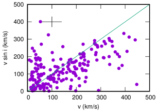
Figure 1: The projected rotation velocity, $v\sin\,i$, as a function of the equatorial rotation velocity, $v$, estimated from the photometric period for stars with effective temperatures $T_{\rm eff}>8000$ K. The straight line is $\sin\,i~{}=~{}1$. The 1-$\sigma$ error bars are shown on the top left.

TESS observations have revealed the rotation frequencies of many more A and B stars for which $v\sin\,i$ measurements are available. Table 2 shows that there are 274 stars with both rotation frequencies and $v\sin\,i$. In Fig. 1 a comparison between $v\sin\,i$ and the photometric $v$ is made for 193 stars with $T_{\rm eff}>8000$ K. The temperature limit was chosen to minimise contamination by stars in which surface convection may still be present. Since $v\sin\,i$ cannot exceed $v$, the points are expected to lie below the $\sin\,i~{}=~{}1$ line in the figure.

The increase in numbers of stars above the $\sin\,i~{}=~{}1$ line at low rotation rates is to be expected. Measurements of $v\sin\,i$ are mostly obtained by measuring the widths of selected spectral lines and applying a calibration to convert to $v\sin\,i$. The calibration is obtained using high-dispersion spectra and modelling line profiles. The error in $v\sin\,i$ is approximately constant at all values of $v\sin\,i$. Analysis of the rotational velocity catalogue of Glebocki & Gnacinski (2005) gives a standard deviation of $v\sin\,i$ of about 30 km s^-1. This means that at low values of $v\sin\,i$, the error is comparable to, or larger, than $v\sin\,i$ itself and many points will lie above the $\sin\,i~{}=~{}1$ line. This is further compounded by the fact that $v\sin\,i$ is constrained to be greater than or equal to zero, although measurements of line width may lead to negative values of $v\sin\,i$ on applying the calibration. As the rotation rate tends to zero, $v\sin\,i$ measurements of ever increasing precision are required to ensure that $v\sin\,i$ stays below the $\sin\,i~{}=~{}1$ line. This is clearly not possible to attain.

Another consideration is that low photometric frequencies are more difficult to measure because a longer time span is required to resolve the frequency peak in the periodogram. Thus instrumental drift becomes important. This is further compounded by the fact that the periodogram noise increases sharply towards zero frequency. Thus the uncertainty in $v$ increases as $v$ approaches zero, contributing to moving the point above the $\sin\,i~{}=~{}1$ line. The standard deviation for $v$ is about 40 km s^-1 as estimated from the errors in $T_{\rm eff}$ and $\log L/L_{\odot}$.

Finally, of course, the possibility exists that some of the stars classified as rotational variables are, in fact, binaries. The distinction between light variability due to binarity effects and rotation was made using two principles. Firstly, stars with low frequencies and amplitudes higher than a few parts per thousand are assumed to be binaries. However, if there is an indication of amplitude variability (seen as broad peaks in the periodogram or amplitude changes in the light curve), then the star is classified as a rotational variable. The distinction becomes increasingly difficult at low frequencies because of instrumental drift and the overall increase in periodogram noise towards low frequencies. Classification becomes more uncertain at low frequencies.

Since most of the stars would be observed at high angles of inclination, a trend between $v\sin\,i$ and $v$ is expected, as seen in Fig. 1. If a linear relationship between $v\sin\,i$ and $v$ is assumed, the probability of the observed correlation occurring by chance, as measured by Student’s t test is less than $10^{-7}$. In actual fact the correlation is not exact because of the $\sin\,i$ factor. If it was possible to take this into account, the correlation will be even higher. The stated probability is thus an upper limit, clearly establishing that a physical effect exists. Whatever is responsible for the photometric variability must be intimately connected with rotation.

It should be noted that there is a inherent difference in the way the rotation rate is measured using $v\sin i$ and the photometric frequency. If the photometric variability is a result of starspots, then there will be a lack of stars with low inclinations because the rotational modulation amplitude tends to zero as $i$ tends to zero. The underlying distribution of stars measured by the two methods is not the same, which means that until we know the distribution of spot sizes and locations, in addition to the distribution of the angles of inclination, there is no possibility of a rigorous statistical test to compare the photometric $v$ with the spectroscopic $v\sin i$.

The equatorial rotation velocity distribution, i.e. the relative number of stars within a particular range of equatorial rotation velocity, is an important quantity which provides information on the physics of stellar rotation. The distribution is expected to vary as a function of effective temperature and gravity due to various factors such as mass loss and evolutionary state. It is obtained from a large number of $v\sin\,i$ measurements of stars within a limited $T_{\rm eff}$ and evolutionary state by deconvolving $v\sin\,i$ assuming random orientation of the axes of rotation. The process requires the inversion of an integral equation (Chandrasekhar & Münch, 1950).

The photometric rotation frequencies, in combination with radii obtained from Gaia DR2 parallaxes, allows the equatorial rotation velocity distribution to be obtained without the need for deconvolution. It should be noted, however, that at low rotation rates the distribution of photometric equatorial rotation velocities, $v$, is not the same as that derived from $v\sin\,i$ after deconvolution. This is due to the fact that rotational modulation cannot be observed at low inclination angles, although $v\sin\,i$ can still be measured. A deficiency of stars at low values of $v$ is expected relative to that obtained from $v\sin\,i$ measurements. The deficiency is increased by the fact that rotation frequencies smaller than about 0.1 d^-1 probably escape detection owing to increased periodogram noise at low frequencies. At high rotation rates, the stellar radius is larger than the mean radius used to determine $v$. It is probable that this affects $v\sin\,i$ in a different way than it does $v$. The question of differential rotation is also likely to affect $v$ and $v\sin\,i$ differently.

Obtaining a distribution requires a large number of stars in order to provide sufficient rotation rate resolution. Fortunately, it is not really necessary to use the same stars in comparing the distributions of $v$ and $v\sin\,i$. It is reasonable to assume that any sample of main sequence stars within a given temperature range will have the same distribution of $v\sin\,i$. Thus one can obtain the $v$ distribution for the 1035 stars with $8000<T_{\rm eff}<10000$ K and compare it with the $v\sin\,i$ distribution of an entirely different, much larger, set of main sequence stars within the same $T_{\rm eff}$ range. Such a test using 875 Kepler A stars in an unrestricted temperature range was made by Balona (2013).

In Fig. 2 the $v$ distributions for stars in three temperature ranges are shown. Also shown are the distributions of $v\sin\,i$ for stars in the same temperature ranges. There are too few stars hotter than 15000 K for a meaningful analysis. Although the two distributions are not directly comparable due to the $\sin i$ factor, there is a clear similarity between them. The tail at rapid rotation rates the number of stars in the $v$ distribution is larger than in the $v\sin i$ distribution. This is expected because at large values of $v$, only a few stars with inclinations very close to equator-on will have large $v\sin\,i$.

One could convolve the $v$ distribution if one knew the distribution of $i$ for the stars measured photometrically. This is not known because we do not know the distribution of sizes and locations of the starspots. As a test, one could simply assume a random distribution of $i$ for $i>30^{\circ}$ with zero for smaller values of $i$. The resulting convolution reduces the numbers of stars in the tails of the $v$ distributions, producing good agreement with the tails of the $v\sin i$ distributions. This does not prove that rotational modulation is involved, but shows that it is not difficult to obtain agreement even in this simple case. Once again, no rigorous statistical test can be made until we have a better knowledge of the underlying distribution of starspot sizes and locations.

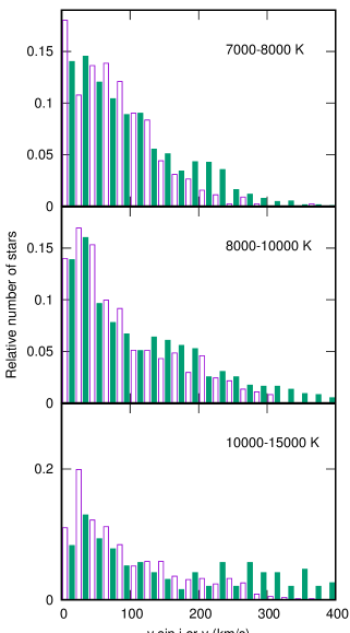
Figure 2: Distribution of projected rotation velocities, $v\sin\,i$ (empty boxes) and equatorial rotation velocities (filled boxes) for stars in different ranges of effective temperature (labelled in degrees K).

The point that is being illustrated in Fig. 2 is that the photometric $v$ measurements give approximately the same rotational velocity distribution as $v\sin\,i$ measurements. This can only be the case if $v$ measures the equatorial rotation velocity or something very close to it, which is a different test from that shown in Fig. 1 and involves many more stars. The implication is that whatever is responsible for the periodic light variation is indistinguishable from rotation. It is found that about 20–40 percent of A and B stars are presumed rotational variables. This fraction increases to 40–60 percent for cooler stars. Thus rotational light modulation, or some other effect indistinguishable from rotational modulation, is very common among all main sequence stars.

4 Discussion

While these results show that a co-rotating feature appears to be present in many hot stars, it is possible that it may not be the same as a sunspot and may not involve a magnetic field. Apart from rotation, there are only two other possibilities which might account for the observations: binarity and pulsation.

Since the observed periods are relatively short, stars in a binary system will be rather close, making eclipses very probable. One would thus expect much higher amplitudes typical of eclipses, not the very low amplitudes of around 100 ppm that are actually observed. Grazing eclipses can only happen in a narrow range of inclination, which is inconsistent with the large fraction of stars observed to vary. Furthermore, the light amplitudes often vary with time, as expected from starspots, but not from eclipsing binaries. Finally, there is the obvious observation that the periods closely agree with the rotation periods and not the orbital periods.

Some form of standing wave might also be considered. Indeed, this idea has been proposed to account for the ROTD feature in the periodogram discussed above. In about 15 percent of Kepler A stars, the periodogram shows a broad hump with a closely-spaced sharp peak at slightly higher frequency (Balona, 2013). It was originally suggested that the broad hump may be due to starspots in differential rotation and the sharp peak a result of a reflection effect from a planet in a synchronous orbit (Balona, 2014). Recently, it has been proposed that the broad peak may be due to Rossby waves, while the sharp peak is due to rotation (Saio et al., 2018). Rossby waves are a subset of inertial waves in a rotating star. It is unlikely that the observed variation is due to Rossby waves alone. In the first place, the sharp peak is identified as the rotational peak, so a starspot is still required in this explanation. Secondly, the majority of periodogram peaks are sharp, while Rossby waves are multiple modes which are expected to lead to broad peaks.

An explanation is required for the low frequencies in A and B stars. If these are not attributed to rotational modulation, it is essential to find an alternative hypothesis. The hypotheses discussed above do not account for the observations and it is therefore reasonable to adopt the rotational modulation idea until a better solution is proposed, even if the consequences are disruptive to current thinking.

Some A stars also appear to flare (Balona, 2012, 2013, 2015). Flares might be expected in any star with spots, and this might be taken as an indication that the spots on A and B stars are similar to those on the Sun. The question of flares in A stars has been disputed on the grounds that the flaring A stars are spectroscopic binaries or that their light curves are contaminated by fainter stars in the same aperture (Pedersen et al., 2017). This could well be true, but the origin of a flare in a multiple system cannot be determined in this way. This can only be done if the stellar disks in the system are resolved. Furthermore, it is insufficient to attribute the flare to one or more contaminating stars. At the very least, it needs to be shown that these stars are of the kind known to flare and that the flare could be sufficiently energetic to be visible in the glare of the A star. It turns out that flares on A stars, which should be called “superflares” in accordance with current usage, attain energies never seen in cool flare stars (Balona, 2013, 2015).

The problems regarding the $\delta$ Scuti stars mentioned above remain unresolved using current ideas of stars with radiative envelopes. If it is assumed that surface convection occurs in all main sequence stars, the presence of starspots in A and B stars is no longer problematical. A thin convective envelope may provide an additional mechanism for pulsational instability which may assist in understanding the low frequencies in $\delta$ Scuti stars.

It has been suggested that magnetic fields produced in subsurface convection zones could appear on the surface (Cantiello et al., 2009; Cantiello & Braithwaite, 2011). As in the Sun, strong localized magnetic fields of opposite polarity lead to a weak global field which would be difficult to detect. Magnetic spots with sizes comparable to the local pressure scale height are predicted to manifest themselves as hot, bright spots. Another possibility is that differential rotation in the A and B stars may be sufficient to create a local magnetic field via dynamo action (Spruit, 1999, 2002; Maeder & Meynet, 2004).

The observations presented here indicate a need for a revision of current understanding of the outer layers of hot stars with radiative envelopes. The ideas discussed above, as well as other possibilities of inducing surface convection in hot stars, should be further explored.

References

- Balona (2011) Balona L. A., 2011, MNRAS, 415, 1691
- Balona (2012) —, 2012, MNRAS, 423, 3420
- Balona (2013) —, 2013, MNRAS, 431, 2240
- Balona (2014) —, 2014, MNRAS, 441, 3543
- Balona (2015) —, 2015, MNRAS, 447, 2714
- Balona (2016) —, 2016, MNRAS, 457, 3724
- Balona (2017) —, 2017, MNRAS, 467, 1830
- Balona (2018) —, 2018, MNRAS, 479, 183
- Balona et al. (2015a) Balona L. A., Baran A. S., Daszyńska-Daszkiewicz J., De Cat P., 2015a, MNRAS, 451, 1445
- Balona et al. (2015b) Balona L. A., Daszyńska-Daszkiewicz J., Pamyatnykh A. A., 2015b, MNRAS, 452, 3073
- Balona et al. (2016) Balona L. A., Engelbrecht C. A., Joshi Y. C., et al., 2016, MNRAS, 460, 1318
- Balona et al. (2019) Balona L. A., Handler G., Chowdhury S., et al., 2019, MNRAS, 485, 3457
- Braithwaite & Spruit (2004) Braithwaite J., Spruit H. C., 2004, Nature, 431, 819
- Brown et al. (2011) Brown T. M., Latham D. W., Everett M. E., Esquerdo G. A., 2011, AJ, 142, 112
- Cantiello & Braithwaite (2011) Cantiello M., Braithwaite J., 2011, A&A, 534, A140
- Cantiello et al. (2009) Cantiello M., Langer N., Brott I., et al., 2009, A&A, 499, 279
- Chandrasekhar & Münch (1950) Chandrasekhar S., Münch G., 1950, ApJ, 111, 142
- Charbonneau (2014) Charbonneau P., 2014, ARA&A, 52, 251
- Gaia Collaboration et al. (2018) Gaia Collaboration, Brown A. G. A., Vallenari A., Prusti T., de Bruijne J. H. J., Babusiaux C., Bailer-Jones C. A. L., 2018, ArXiv e-prints
- Gaia Collaboration et al. (2016) Gaia Collaboration, Prusti T., de Bruijne J. H. J., et al., 2016, A&A, 595, A1
- Glebocki & Gnacinski (2005) Glebocki R., Gnacinski P., 2005, VizieR Online Data Catalog, 3244
- Gontcharov (2017) Gontcharov G. A., 2017, Astronomy Letters, 43, 472
- Grigahcène et al. (2010) Grigahcène A., Antoci V., Balona L., et al., 2010, ApJ, 713, L192
- Maeder & Meynet (2004) Maeder A., Meynet G., 2004, A&A, 422, 225
- Michaud et al. (1976) Michaud G., Charland Y., Vauclair S., Vauclair G., 1976, ApJ, 210, 447
- Mowlavi et al. (2013) Mowlavi N., Barblan F., Saesen S., Eyer L., 2013, A&A, 554, A108
- Pecaut & Mamajek (2013) Pecaut M. J., Mamajek E. E., 2013, ApJS, 208, 9
- Pedersen et al. (2017) Pedersen M. G., Antoci V., Korhonen H., White T. R., Jessen-Hansen J., Lehtinen J., Nikbakhsh S., Viuho J., 2017, MNRAS, 466, 3060
- Petit et al. (2011) Petit P., Lignières F., Wade G. A., Aurière M., Alina D., Böhm T., Oza A., 2011, Astronomische Nachrichten, 332, 943
- Saio et al. (2018) Saio H., Kurtz D. W., Murphy S. J., Antoci V. L., Lee U., 2018, MNRAS, 474, 2774
- Samus et al. (2009) Samus N. N., Durlevich O. V., et al., 2009, VizieR Online Data Catalog, 1, 2025
- Skiff (2014) Skiff B. A., 2014, VizieR Online Data Catalog, 1, 2023
- Spruit (1999) Spruit H. C., 1999, A&A, 349, 189
- Spruit (2002) —, 2002, A&A, 381, 923
- Vanderburg & Johnson (2014) Vanderburg A., Johnson J. A., 2014, PASP, 126, 948