Int-Deep: A Deep Learning Initialized Iterative Method for Nonlinear Problems

Abstract

This paper proposes a deep-learning-initialized iterative method (Int-Deep) for low-dimensional nonlinear partial differential equations (PDEs). The corresponding framework consists of two phases. In the first phase, an expectation minimization problem formulated from a given nonlinear PDE is approximately resolved with mesh-free deep neural networks to parametrize the solution space. In the second phase, a solution ansatz of the finite element method to solve the given PDE is obtained from the approximate solution in the first phase, and the ansatz can serve as a good initial guess such that Newton’s method or other iterative methods for solving the nonlinear PDE are able to converge to the ground truth solution with high-accuracy quickly. Systematic theoretical analysis is provided to justify the Int-Deep framework for several classes of problems. Numerical results show that the Int-Deep outperforms existing purely deep learning-based methods or traditional iterative methods (e.g., Newton’s method and the Picard iteration method).

Keywords. Deep learning, nonlinear problems, partial differential equations, eigenvalue problems, iterative methods, fast and accurate.

AMS subject classifications: 68U99, 65N30 and 65N25.

1 Introduction

This paper is concerned with the efficient numerical method for solving nonlinear partial differential equations (PDEs) including a class of eigenvalue problems as special cases, which is a ubiquitous and important topic in science and engineering [23, 3, 30, 36, 8, 42, 31, 15]. As far as we know, there have developed many traditional and typical numerical methods in this area, e.g., the finite difference method, the spectral method, and the finite element method [46]. The first two methods are generally used for solving problems over regular domains while the latter one is particularly suitable for solving problems over irregular domains [7, 67]. To achieve the numerical solution with the desired accuracy, one is often required to numerically solve the discrete problem formulated as a large-scale nonlinear system of nonlinear equations, which is time-consuming. In this case, one of the most critical issues is to choose the feasible initial guess so that the numerical solver (e.g. Newton’s method) is convergent. On the other hand, for reducing the computational cost, two grid methods are thereby devised in [58, 59], which only require to solve a small-sized nonlinear system arising from the finite element discretization based on a coarse triangulation. However, the difficulty is that we even can not ensure if the nonlinear system has a solution in theory if the mesh size of the coarse triangulation is large enough.

Recently, science and engineering have undergone a revolution driven by the success of deep learning techniques that originated in computer science. This revolution also includes broad applications of deep learning in computational and applied mathematics. Many new branches in scientific computing have emerged based on deep learning in the past five years including new methods for solving nonlinear PDEs. There are mainly two kinds of deep learning approaches for solving non-linear PDEs: mesh-based [55, 56, 32, 34, 21, 20, 22] and mesh-free [9, 14, 28, 33, 48, 53, 47]. In the mesh-based methods, deep neural networks (DNNs) are constructed to approximate the solution operator of a PDE, e.g., seeking a DNN that approximates the map mapping the coefficients (or initial/boundary conditions) of a PDE to the corresponding solution. After construction, the DNN can be applied to solve a specific class of PDEs efficiently. In the mesh-free methods, which probably date back to 1990’s (e.g., see [17, 38]), DNNs are applied as the parametrization of the solution space of a PDE; then the solution of the PDE is identified via seeking a DNN that fits the constraints of the PDE in the least-squares sense or minimizes a variational problem formulated from PDEs. The key to the success of these approaches is the universal approximation capacity of DNNs [37, 6, 61, 62, 52] even without the curse of dimensionality for a large class of functions [6, 43, 45, 44, 39].

Though the deep learning approach has made it possible to solve high-dimensional problems, which is a significant breakthrough in scientific computing, to the best of our knowledge, the advantage of deep learning approaches over traditional methods in the low-dimensional region is still not clear yet. The main concern is the computational efficiency of these frameworks: the number of iterations in deep learning methods is usually large or the accuracy is very limited (e.g., typically $10^{-2}$ to $10^{-4}$ relative error). In order to overcome this difficulty, one is tempted to set up a more efficient neural network architecture (e.g., incorporating physical information in the structure designing [49, 57, 64, 21, 27], designing a more advanced learning algorithm for deep learning training [41, 63], or using a solution ansatz according to prior knowledge [38, 50, 40]). However, the overall performance of these frameworks for nonlinear problems without any prior knowledge may still not be very convincingly efficient.

This paper proposes the Int-Deep framework from a new point of view for designing highly efficient solvers of low-dimensional nonlinear PDEs with a finite element accuracy leveraging both the advantages of traditional algorithms and deep learning approaches. The Int-Deep framework consists of two phases as shown in Figure 1. In the first phase, an approximate solution to the given nonlinear PDE is obtained via deep learning approaches using DNNs of size $O(1)$ and $O(100)$ iterations, where $O(\cdot)$ means that the prefactor is independent of the final target accuracy in the Int-Deep framework, i.e., the accuracy of finite element methods. In particular, based on variational principles, we propose new methods to formulate the problem of solving nonlinear PDEs into an unconstrained minimization problem of an expectation over a function space parametrized via DNNs, which can be solved efficiently via batch stochastic gradient descent (SGD) methods due to the special form of expectation. Unlike previous methods in which the form of expectation is only derived for nonlinear PDEs related to variational equations, our proposed method can also handle those related to variational inequalities, providing a unified variational framework for a wider range of nonlinear problems.

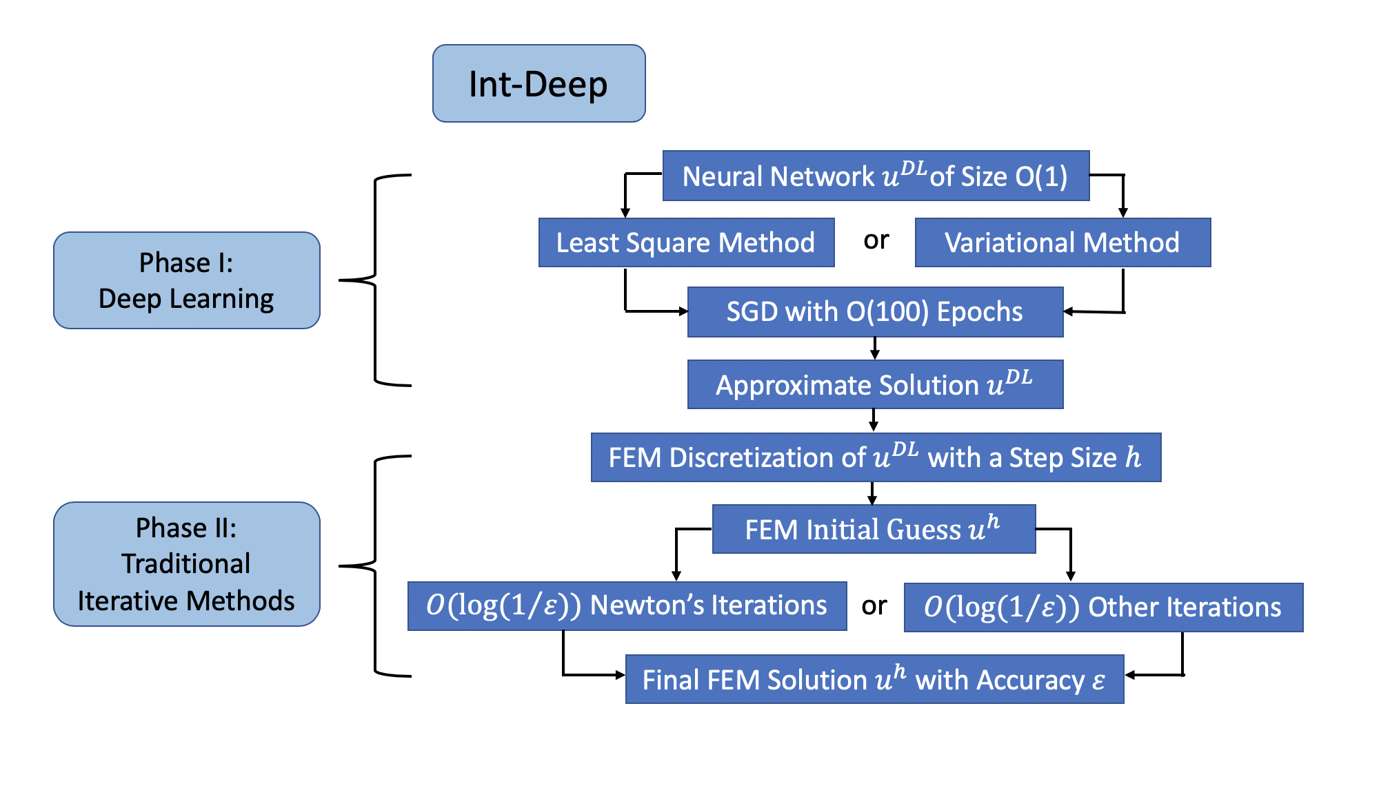
Figure 1: Computational flow of Int-Deep: Deep learning solvers in Phase I only require $O(1)$ computational cost since the network size is $O(1)$ and the number of epochs of the stochastic gradient descent (SGD) is $O(100)$. Empirically, traditional iterative methods converges to a solution with $O(\epsilon)$ accuracy in $O(\log(\frac{1}{\epsilon}))$ iterations in Phase II.

In the second phase, the approximate solution provided by deep learning approaches can serve as a good initial guess such that traditional iterative methods (e.g., Newton’s method for solving nonlinear PDEs and the shifted power method for eigenvalue problems) converge quickly to the ground truth solution with high-accuracy. The hybrid algorithm substantially reduces the learning cost of deep learning approach while keeping the quality of initial guesses for traditional iterative methods; good initial guesses enable traditional iterative methods to converge in $O(\log(\frac{1}{\epsilon}))$ iterations to the $\epsilon$ precision of finite element methods. In each iteration of the traditional iterative method, the nonlinear problem has been linearized and hence traditional fast solvers for linear systems can be applied depending on the underlying structure of the linear system. Therefore, as we shall see in the numerical section, the Int-Deep framework outperforms existing purely deep learning-based methods or traditional iterative methods, e.g., Newton’s method and Picard iteration. Furthermore, systematic theoretical analysis is provided to characterize the conditions under which the Int-Deep framework converges, serving as a trial to change current deep learning research from trial-and-error to a suite of methods informed by a principled design methodology.

This paper will be organized as follows. In Section 2, we briefly review the definitions of DNNs. In Section 3, we introduce the expectation minimization framework for deep learning-based PDE solvers in the first phase of the Int-Deep framework. In Section 4, as the second phase of Int-Deep, traditional iterative methods armed with good initial guesses provided by deep learning approaches will be introduced together with its theoretical convergence analysis, for clarity of presentation the proofs of which are left in Appendix. In Section 5, a set of numerical examples will be provided to demonstrate the efficiency of the proposed framework and to justify our theoretical analysis. Finally in Section 6, we summarize our paper with a short discussion.

2 Deep Neural Networks (DNNs)

Mathematically, DNNs are a form of highly non-linear function parametrization via function compositions using simple non-linear functions [26]. The validity of such an approximation method can be ensured by the universal approximation theorems of DNNs in [37, 6, 61, 62, 51, 52]. Let us introduce two basic neural network structures commonly used for solving PDEs below.

The first one is the so-called fully connected feed-forward neural network (FNN), which is a function in the form of a composition of $L$ simple nonlinear functions as follows:

$$\phi(\bm{x};\bm{\theta}):=\bm{a}^{T}\bm{h}_{L}\circ\bm{h}_{L-1}\circ\cdots\circ\bm{h}_{1}(\bm{x}),$$

where $\bm{h}_{\ell}(\bm{x})=\sigma\left(\bm{W}_{\ell}\bm{x}+\bm{b}_{\ell}\right)$ with $\bm{W}_{\ell}\in\mathbb{R}^{N_{\ell}\times N_{\ell-1}}$, $\bm{b}_{\ell}\in\mathbb{R}^{N_{\ell}}$ for $\ell=1,\dots,L$, $\bm{a}\in\mathbb{R}^{N_{L}}$, $\sigma$ is a non-linear activation function, e.g., a rectified linear unit (ReLU) $\sigma(x)=\max\{x,0\}$ or hyperbolic tangent function $\tanh(x)$. Each $\bm{h}_{\ell}$ is referred as a hidden layer, $N_{\ell}$ is the width of the $\ell$-th layer, and $L$ is called the depth of the FNN. In the above formulation, $\bm{\theta}:=\{\bm{a},\,\bm{W}_{\ell},\,\bm{b}_{\ell}:1\leq\ell\leq L\}$ denotes the set of all parameters in $\phi$, which uniquely determines the underlying neural network.

The second one is the so-called residual neural network (ResNet) introduced by He, Zhang, Ren and Sun in [29]. We apply its variant defined recursively as follows:

$$\bm{h}_{0} = \bm{V}\bm{x},$$

$$\bm{g}_{\ell} = \sigma(\bm{W}_{\ell}\bm{h}_{\ell-1}+\bm{b}_{\ell}),\qquad\ell=1,2,\dots,L,$$

$$\bm{h}_{\ell} = \bm{\bar{U}}_{\ell}\bm{h}_{\ell-2}+\bm{U}_{\ell}\bm{g}_{\ell},\quad\ell=1,2,\dots,L,$$

$$\phi(\bm{x};\bm{\theta}) = \bm{a}^{T}\bm{h}_{L},$$

where $\bm{V}\in\mathbb{R}^{N_{0}\times d}$, $\bm{W}_{\ell}\in\mathbb{R}^{N_{\ell}\times N_{0}}$, $\bm{\bar{U}}_{\ell}\in\mathbb{R}^{N_{0}\times N_{0}}$, $\bm{U}_{\ell}\in\mathbb{R}^{N_{0}\times N_{\ell}}$, $\bm{b}_{\ell}\in\mathbb{R}^{N_{\ell}}$ for $\ell=1,\dots,L$, $\bm{a}\in\mathbb{R}^{N_{0}}$, $\bm{h}_{-1}=\bm{0}$. Throughout this paper, we consider $N_{0}=N_{\ell}=N$ and $\bm{U}_{\ell}$ is set as the identity matrix in the numerical implementation of ResNets for the purpose of simplicity. Furthermore, as used in [19], we set $\bm{\bar{U}}_{\ell}$ as the identify matrix when $\ell$ is even and set $\bm{\bar{U}}_{\ell}=\bm{0}$ when $\ell$ is odd.

3 Phase I of Int-Deep: Variational Formulas for Deep Learning

In this section, we will present existing and our new analysis for reformulating nonlinear PDEs including eigenvalue problems to the minimization of expectation that can be solved by SGD. The analysis works for PDEs related to variational equations and variational inequalities, the latter of which is of special interest since there might be no available literature discussing this case to the best of our knowledge. Hence, our analysis could serve as a good reference for a wide range of problems.

Throughout this paper, we will use standard symbols and notations for Sobolev spaces and their norms/seminorms; we refer the reader to the reference [1] for details. Moreover, the standard $L^{2}(D)$-inner product for a bounded domain $D$ is denoted by $(\cdot,\cdot)_{D}$. If the domain $D$ is the solution domain $\Omega$, we will drop out the dependence of $\Omega$ in all Sobolev norms/seminorms and $L^{2}(\Omega)$-inner product when there is no confusion caused.

3.1 PDE Solvers Based on DNNs

The general idea of deep learning-based PDE solvers is to treat DNNs as an efficient parametrization of the solution space of a PDE and the solution of the PDE is identified via seeking a DNN that fits the constraints of the PDE in the least-squares sense or minimizes the variational minimization problem related to the PDE. Let us use the following example to illustrate the main idea:

$$\left\{\begin{aligned} \mathcal{D}(u)&=f\quad\text{in }\Omega,\\ \mathcal{B}(u)&=g\quad\text{on }\partial\Omega,\end{aligned}\right.$$ (3.1)

where $\mathcal{D}$ is a differential operator and $\mathcal{B}$ is a boundary operator.

In the least squares type methods (LSM), a DNN $\phi(\bm{x};\bm{\theta}^{*})$ is constructed to approximate the solution $u(\bm{x})$ for $\bm{x}\in\Omega$ via minimizing the square loss

$$\bm{\theta}^{*}=\operatorname*{arg\,min}_{\bm{\theta}}\mathcal{L}(\bm{\theta}):=\mathbb{E}_{\bm{x}\in\Omega}\left[\left|\mathcal{D}\phi(\bm{x};\bm{\theta})-f(\bm{x})\right|^{2}\right]+\gamma\mathbb{E}_{\bm{x}\in\partial\Omega}\left[\left|\mathcal{B}\phi(\bm{x};\bm{\theta})-g(\bm{x})\right|^{2}\right],$$ (3.2)

with a positive parameter $\gamma$.

In the variational type methods (VM), (3.1) is solved via a variational minimization

$$u^{*}=\operatorname*{arg\,min}_{u\in H}J(u),$$ (3.3)

where the Hilbert space $H$ is an admissible space, and $J(u)$ is a nonlinear functional over $H$. Then, the solution space $H$ is parametrized via DNNs, i.e., $H\approx\{\phi(\bm{x};\bm{\theta})\}_{\bm{\theta}}$, where $\phi$ is a DNN with a fixed depth $L$ and width $N$. After parametrization, (3.3) is approximated by the following problem:

$$\bm{\theta}^{*}=\operatorname*{arg\,min}_{\bm{\theta}}J(\phi(\bm{x};\bm{\theta})).$$ (3.4)

In general, $J(\phi(\bm{x};\bm{\theta}))$ can be formulated as the sum of several integrals over several sets $\{\Omega_{i}\}_{i=1}^{p}$, each of which corresponds to one equation in (3.1):

$$J(\phi(\bm{x};\bm{\theta}))=\sum_{i=1}^{p}\int_{\Omega_{i}}F_{i}(\bm{x};\bm{\theta})\,{\rm d}x=\sum_{i=1}^{p}|\Omega_{i}|\mathbb{E}_{\bm{\xi}_{i}}\Big{[}F_{i}(\bm{\xi}_{i};\bm{\theta})\Big{]},$$ (3.5)

where $F_{i}(\cdot;\bm{\theta)}$ is a function related to a variational constraint on $\phi(\bm{x};\bm{\theta})$, $\bm{\xi}_{i}$ is a random vector produced by the uniform distribution over $\Omega_{i}$, and $|\Omega_{i}|$ denotes the measure of $\Omega_{i}$. In addition, $\bm{\xi}_{i}$ ($1\leq i\leq p$) are mutually independent. Based on (3.5), (3.4) can be expressed as

$$\bm{\theta}^{*}=\operatorname*{arg\,min}_{\bm{\theta}}\sum_{i=1}^{p}|\Omega_{i}|\mathbb{E}_{\bm{\xi}_{i}}\Big{[}F_{i}(\bm{\xi}_{i};\bm{\theta})\Big{]}.$$ (3.6)

Both the LSM in (3.2) and VM in (3.4) can be reformulated to the expectation minimization problem in (3.6), which can be solved by the stochastic gradient descent (SGD) method or its variants (e.g., Adam [35]). In this paper, we refer to (3.6) as the expectation minimization framework for PDE solvers based on deep learning.

Although the convergence of SGD for minimizing the expectation in (3.6) is still an active research topic, empirical success shows that SGD can provide a good approximate local minimizer of (3.2) and (3.6). This completes the algorithm of using deep learning to solve nonlinear PDEs with equality constraints.

We would like to emphasize that when the PDE in (3.1) is nonlinear, its solutions might be the saddle points of (3.5) making it very challenging to identify its solutions via minimizing (3.5). Hence, we will use the LSM in (3.2) for PDEs associated with variational equations. It deserves to point out that (3.2) is also regarded as a variational formulation, referred to as the least-squares variational principle in [10] in contrast with the usual Ritz variational principle.

3.2 Minimization Problems for Variational Inequalities

Variational inequalities are a class of important nonlinear problems, frequently encountered in various industrial and engineering applications [18, 25]. Unlike previous methods in which the form of expectation is only derived for nonlinear PDEs with variational equations, we propose an expectation minimization framework also suitable for variational inequalities.

The abstract framework of an elliptic variational inequality of the second kind can be described as follows (cf. [25]). Find $u\in H$ such that

$$a(u,v-u)+j(v)-j(u)\geq\langle f,v-u\rangle,\quad v\in H,$$ (3.7)

where $H$ is a Hilbert space equipped with the norm $\|\cdot\|_{H}$, and $\langle\cdot,\cdot\rangle$ stands for the duality pairing between $H^{\prime}$ and $H$, with $H^{\prime}$ being the dual space of $H$; $a(\cdot,\cdot)$ is a continuous, coercive and symmetric bilinear form over $H$; $j(\cdot):H\rightarrow\mathbb{\overline{R}}=\mathbb{R}\cup\{\pm\infty\}$ is a proper, convex and lower semi-continuous functional.

As shown in [25], the above problem has a unique solution under the stated conditions on the problem data. Moreover, it can be reformulated as the following minimization problem:

$$u=\operatorname*{arg\,min}_{v\in H}J(v)=\frac{1}{2}a(v,v)-\langle f,v\rangle+j(v),$$ (3.8)

which naturally falls into our expectation minimization framework in (3.6).

Let us discuss the simplified friction problem as an example, where the nonlinear PDE is given by

$$\begin{cases}-\Delta u+u=f\quad&\mbox{in}\ \Omega,\\ |\partial_{\bm{n}}u|\leq g,\ u\partial_{\bm{n}}u+g|u|=0\quad&\mbox{on}\ \Gamma_{C},\\ u=0\quad&\mbox{on}\ \Gamma_{D},\end{cases}$$ (3.9)

where $\bm{n}$ is the unit outward normal to $\partial\Omega$; $\Gamma_{C}\subset\partial\Omega$ denotes the friction boundary, and $\Gamma_{D}=\partial\Omega\setminus\Gamma_{C}$; $f\in L^{2}(\Omega)$ and $g\in L^{2}(\Gamma_{C})$ are two given functions. (3.9) can be expressed as an elliptic variational inequality in the form (3.7) or (3.8) by choosing

$$H=V_{D}=\{\phi\in H^{1}(\Omega):\phi=0\ \mbox{on}\ \Gamma_{D}\}$$

and

$$a(\phi,\chi)=(\nabla\phi,\nabla\chi)+(\phi,\chi),\quad j(\phi)=(g,|\phi|)_{\Gamma_{C}},\quad\phi,\;\chi\in V_{D}.$$

Hence, the minimization problem of the nonlinear PDE (3.9) is given by

$$u=\operatorname*{arg\,min}_{\phi\in V_{D}}J_{1}(\phi),$$ (3.10)

where

$$J_{1}(\phi) =\frac{1}{2}\|\phi\|_{1}^{2}-(f,\phi)+j(\phi)$$

$$=|\Omega|\mathbb{E}_{\bm{\xi}_{1}}\Big{[}\frac{1}{2}\big{(}|\nabla_{\bm{\xi}_{1}}\phi(\bm{\xi}_{1};\bm{\theta})|^{2}+\phi^{2}(\bm{\xi}_{1};\bm{\theta})\big{)}-f(\bm{\xi}_{1})\phi(\bm{\xi}_{1};\bm{\theta})\Big{]}+|\Gamma_{C}|\mathbb{E}_{\bm{\xi}_{2}}\Big{[}g(\bm{\xi}_{2})|\phi(\bm{\xi}_{2};\bm{\theta})|\Big{]},$$

where $\bm{\xi}_{1}$ and $\bm{\xi}_{2}$ are random vectors following the uniform distribution over $\Omega$ and $\Gamma_{C}$, respectively.

We can also use the penalty method to remove the constraint condition in the admissible space $V_{D}$, giving rise to an easier unconstrained minimization problem for deep learning. Then, the problem (3.10) is modified as

$$u=\operatorname*{arg\,min}_{\phi\in V_{1}}J_{2}(\phi),$$ (3.11)

where

$$V_{1}=H^{1}(\Omega)\quad J_{2}(\phi)=J_{1}(\phi)+\gamma\|\phi\|_{0,\Gamma_{D}}^{2} =|\Omega|\mathbb{E}_{\bm{\xi}_{1}}\Big{[}\frac{1}{2}\big{(}|\nabla_{\bm{\xi}_{1}}\phi(\bm{\xi}_{1};\bm{\theta})|^{2}+\phi^{2}(\bm{\xi}_{1};\bm{\theta})\big{)}-f(\bm{\xi}_{1})\phi(\bm{\xi}_{1};\bm{\theta})\Big{]}$$

$$\quad+|\Gamma_{C}|\mathbb{E}_{\bm{\xi}_{2}}\Big{[}g(\bm{\xi}_{2})|\phi(\bm{\xi}_{2};\bm{\theta})|\Big{]}+|\Gamma_{D}|\mathbb{E}_{\bm{\xi}_{3}}\Big{[}\gamma\phi^{2}(\bm{\xi}_{3};\bm{\theta})\Big{]},$$

with $\gamma$ denoting a penalty parameter to be determined feasibly and $\bm{\xi}_{3}$ being a random vector following the uniform distribution over $\Gamma_{D}$. The minimization problem in (3.11) is of the form of expectation minimization in (3.6).

3.3 Minimization Problems for Eigenvalue Problems

Now we discuss how to evaluate the smallest eigenvalue and its eigenfunction for a positive self-adjoint differential operator, e.g.,

$$\begin{cases}-\nabla(p(\bm{x})\nabla u)+q(\bm{x})u=\lambda u\quad&\mbox{in}\ \Omega,\\ u=0\quad&\mbox{on}\ \partial\Omega,\end{cases}$$ (3.12)

where $p(\bm{x})\in C^{1}(\bar{\Omega})$ and there exist two positive constants $p_{1}\geq p_{0}$ such that $p_{0}\leq p(\bm{x})\leq p_{1}$ for all $\bm{x}\in\bar{\Omega}$, and $q(\bm{x})\in C(\bar{\Omega})$ is nonnegative over $\Omega$. Here and in what follows, $\bar{\Omega}$ denotes the closure of $\Omega$.

The solution $(\lambda,u)$ is governed by the following variational problem

$$u=\operatorname*{arg\,min}_{\phi\in V}J_{3}(\phi),$$ (3.13)

where $V=H_{0}^{1}(\Omega)$ and

$$J_{3}(\phi)=\frac{a(\phi,\phi)}{\|\phi\|_{0}^{2}}+\gamma(\phi(\bm{x}_{0})-1)^{2};\quad a(\phi,\chi)=\int_{\Omega}[p(\bm{x})\nabla\phi\cdot\nabla\chi+q(\bm{x})\phi\ \chi]\,{\rm d}x,\quad\phi,\ \chi\in V;$$

$\gamma$ is any given positive number, and $\bm{x}_{0}$ is any given point in the interior of $\Omega$.

If $u_{*}\in V$ is a solution, we have by the variational principle for eigenvalue problems [2] that

$$u_{*}=\operatorname*{arg\,min}_{\phi\in V}\frac{a(\phi,\phi)}{\|\phi\|_{0}^{2}}.$$ (3.14)

Let $\alpha$ be a constant such that $(\alpha u_{*})(\bm{x}_{0})=1$ and $u=\alpha u_{*}$. By (3.14), $J_{3}(u)\leq\frac{a(\phi,\phi)}{\|\phi\|_{0}^{2}}\leq J_{3}(\phi)$ for all $\phi\in V$. The converse can be proved similarly. Furthermore, it is easy to check that

$$J_{3}(\phi)=\frac{a(\phi(\bm{x};\bm{\theta}),\phi(\bm{x};\bm{\theta}))}{\|\phi(\bm{x};\bm{\theta})\|_{0}^{2}}+\gamma(\phi(\bm{x}_{0};\bm{\theta})-1)^{2}{=\frac{\mathbb{E}_{\bm{\xi}}\Big{[}p(\bm{\xi})|\nabla_{\bm{\xi}}\phi(\bm{\xi};\bm{\theta})|^{2}+q(\bm{\xi})\phi^{2}(\bm{\xi};\bm{\theta})\Big{]}}{\mathbb{E}_{\bm{\eta}}\Big{[}\phi^{2}(\bm{\eta};\bm{\theta})\Big{]}}+\gamma(\phi(\bm{x}_{0};\bm{\theta})-1)^{2},}$$

where $\bm{\xi}$ and $\bm{\eta}$ are i.i.d. random vectors following the uniform distribution over $\Omega$.

In fact, (3.13) is a constrained minimization problem, that is

$$u=\operatorname*{arg\,min}_{\phi\in V_{1}}J_{3}(\phi),$$

s.t. $$u=0\quad\mbox{on}\ \partial\Omega,$$

where $V_{1}=H^{1}(\Omega)$ as before. Here, we exploit the idea from Jens Berg and Kaj Nystr$\ddot{\text{o}}$m [9] to reformulate the above problem as an unconstrained minimization one. To this end, we construct the neural network function as follows:

$$\phi(\bm{x};\bm{\theta})=B(\bm{x})\psi(\bm{x};\bm{\theta}),$$

where $B(\bm{x})$ is a known smooth function such that the boundary $\partial\Omega$ can be parametrized by $B(\bm{x})=0$, and $\psi(\bm{x};\bm{\theta})$ is any function in $V_{1}$. So (3.13) becomes the expectation minimization:

$$u=\operatorname*{arg\,min}_{\psi\in V_{1}}J_{3}(B(\bm{x})\psi(\bm{x};\bm{\theta})).$$ (3.15)

Once we have obtained the eigenfunction $u(\bm{x})$, the corresponding eigenvalue is $\lambda=a(u,u)/\|u\|_{0}^{2}$. Note that the variational formulation developed here is different from the one devised by E and Yu [19] and the expectation form in our formulation makes it easier to implement SGD.

The proposed method evaluates the smallest eigenvalue and its eigenfunction not only for linear eigenvalue problems, but also for nonlinear eigenvalue problems. To generalize this idea for nonlinear eigenvalue problems, let us consider the nonlinear Schr$\ddot{\text{o}}$dinger equation called the Gross-Pitaevskii (GP) equation as an example:

$$\begin{cases}-\Delta u+V(\bm{x})u+\beta u^{3}=\lambda u&\quad\mbox{in}\ \Omega,\\ u=0&\quad\mbox{on}\ \partial\Omega,\\ \|u\|_{0}=1,\end{cases}$$ (3.16)

where the real-valued potential function $V(\bm{x})\in L^{p}(\Omega)$ for some real number $p>1$, and $\beta$ is a positive number.

According to [13], the ground state non-negative solution $(\lambda,u)$ of (3.16) is unique and governed by the following variational problem

$$u=\operatorname*{arg\,min}\{J_{4}(\phi):\phi\in H_{0}^{1}(\Omega),\|\phi\|_{0}=1\},$$ (3.17)

where

$$J_{4}(\phi)=(\nabla\phi,\nabla\phi)+(V(\bm{x})\phi,\phi)+\frac{\beta}{2}(\phi^{3},\phi).$$

To relax the constraint $\|\phi\|_{0}=1$, we consider the minimization problem for $\phi/\|\phi\|_{0}$ with $\phi\in V$, and reformulate the variational problem (3.17) in the form

$$u=\operatorname*{arg\,min}_{\phi\in H_{0}^{1}(\Omega)}J_{5}(\phi),$$ (3.18)

where

$$J_{5}(\phi)=\frac{(\nabla\phi,\nabla\phi)+(V(\bm{x})\phi,\phi)}{\|\phi\|_{0}^{2}}+\frac{\beta}{2}\frac{(\phi^{3},\phi)}{\|\phi\|_{0}^{4}}+\gamma(\phi(\bm{x}_{0})-1)^{2};$$

$\bm{x}_{0}$ is any given point in the interior of $\Omega$. Moreover, the functional $J_{5}(\phi)$ can be written as the expectation framework as follow.

$$J_{5}(\phi(\bm{x};\bm{\theta})) =\frac{(\nabla_{\bm{x}}\phi(\bm{x};\bm{\theta}),\nabla_{\bm{x}}\phi(\bm{x};\bm{\theta}))+(V(\bm{x})\phi(\bm{x};\bm{\theta}),\phi(\bm{x};\bm{\theta}))}{\|\phi(\bm{x};\bm{\theta})\|_{0}^{2}}+\frac{\beta}{2}\frac{(\phi^{3}(\bm{x};\bm{\theta}),\phi(\bm{x};\bm{\theta}))}{\|\phi(\bm{x};\bm{\theta})\|_{0}^{4}}$$

$$\quad+\gamma(\phi(\bm{x}_{0};\bm{\theta})-1)^{2}$$

$$=\frac{\mathbb{E_{\bm{\xi}}}\Big{[}|\nabla_{\bm{\xi}}\phi(\bm{\xi};\bm{\theta})|^{2}+V(\bm{\xi})\phi^{2}(\bm{\xi};\bm{\theta})\Big{]}}{\mathbb{E_{\bm{\eta}}}\Big{[}\phi^{2}(\bm{\eta};\bm{\theta})\Big{]}}+\frac{\beta}{2|\Omega|}\frac{\mathbb{E_{\bm{\xi}}}\Big{[}\phi^{4}(\bm{\xi};\bm{\theta})\Big{]}}{\mathbb{E_{\bm{\eta};\bm{\zeta}}}\Big{[}\phi^{2}(\bm{\eta};\bm{\theta})\phi^{2}(\bm{\zeta};\bm{\theta})\Big{]}}+\gamma(\phi(\bm{x}_{0};\bm{\theta})-1)^{2},$$

where $\bm{\xi},\bm{\eta},\bm{\zeta}$ are i.i.d. random vectors produced by the uniform distribution over $\Omega$.

Similarly, we can also eliminate the boundary constraint following the ideas in linear eigenvalue problems. Then the variational problem (3.17) is rewritten as

$${u=\operatorname*{arg\,min}_{\psi\in V_{1}}J_{5}(B(\bm{x})\psi(\bm{x};\theta)),}$$ (3.19)

where $V_{1}=H^{1}(\Omega)$ and $B(\bm{x})$ is the same as of linear eigenvalue problems.

It is noted that if $u$ is the solution of (3.19), the eigenfunction is its normalization: $u/\|u\|_{0}$ (still denoted by $u$ for simplicity). Thus, the smallest eigenvalue can be computed by

$$\lambda=(\nabla_{\bm{x}}u,\nabla_{\bm{x}}u)+(V(\bm{x})u,u)+\beta(u^{3},u).$$

4 Phase II of Int-Deep: Traditional Iterative Methods

We propose to use deep learning solutions as initial guesses so as to achieve a high-accurate solution by traditional iterative methods in a few iterations (e.g., Newton’s method for solving nonlinear systems [54][24] or the two grid methods in the context of finite elements [58, 59, 60][12]). In fact, these ideas have led to high-performance methods for solving semilinear elliptic problems and eigenvalue problems with the effectiveness shown by mathematical theory and numerical simulation. The key analysis of this idea is to characterize the conditions under which deep learning solutions can help traditional iterative methods converge quickly. We will provide several classes of examples and the corresponding analysis to support this idea as follows. In what follows, $u^{DL}$ denotes the numerical solution obtained by the deep learning algorithm, and $I_{h}$ is the usual nodal interpolation operator (cf. [11, 16]).

4.1 Semilinear Elliptic Equations with Equality Constrains

Consider the following semilinear elliptic equation

$$\begin{cases}-\Delta u+f(\bm{x},u)=0&\quad\mbox{in}\;\Omega,\\ u=0&\quad\mbox{on}\;\partial\Omega,\end{cases}$$ (4.1)

where $\Omega$ is a bounded convex polygon in $\mathbb{R}^{d}$ ($d=1,2$), and $f(\bm{x},u)$ is a sufficiently smooth function. For simplicity, we use $f(u)$ for $f(\bm{x},u)$ and $f^{\prime}$ for $f_{u}$ in what follows.

Let $V=H_{0}^{1}(\Omega)$. Then the variational formulation of problem (4.1) is to find $u\in V$ such that

$$a(u,\chi):=(\nabla u,\nabla\chi)+(f(u),\chi)=0,\quad\chi\in V.$$ (4.2)

For any $v\in L^{\infty}(\Omega)$, define

$$a_{v}(\phi,\chi):=(\nabla\phi,\nabla\chi)+(f^{\prime}(v)\phi,\chi),\quad\phi,\ \chi\in V.$$ (4.3)

As in [58, 59], we assume that problem (4.1) (equivalently, problem (4.2)) satisfies the following conditions:

• Any solution $u$ of (4.1) has the regularity $u\in W^{2,\infty}(\Omega)$.

• Let $u\in W^{2,\infty}(\Omega)$ be a solution of (4.1). Then there exists a positive constant $C^{u}$ such that

  $$C^{u}\|\phi\|_{1}\leq\sup_{\chi\in V}\frac{a_{u}(\phi,\chi)}{\|\chi\|_{1}},\quad\phi\in V.$$

We next consider the finite element method for solving problem (4.2). Let $\mathcal{T}_{h}$ be a quasi-uniform and shape regular triangulation of $\Omega$ into $K$. Write $h_{K}=\text{diam}(K)$ and $h:=\max_{K\in\mathcal{T}_{h}}h_{K}$. Introduce the Courant element space by

$$V_{h}=\{\phi\in C(\bar{\Omega}):\phi|_{K}\in\mathbb{P}_{1}(K)\mbox{ for all }K\in\mathcal{T}_{h}\}\cap V,$$ (4.4)

where $\mathbb{P}_{1}(K)$ denotes the function space consisting of all linear polynomials over $K$. Then the finite element method is to find $u^{h}\in V_{h}$ such that

$$a(u^{h},\chi)=0,\quad\chi\in V_{h}.$$ (4.5)

Now, let us introduce Int-Deep for solving the problem in (4.5). Concretely speaking, we choose $I_{h}u^{DL}$ as the initial guess and obtain a highly accurate approximate solution by Newton’s method.

Algorithm 1 A hybrid Newton’s method for semilinear problems

Input: the target accuracy $\epsilon$, the maximum number of iterations $N_{\max}$, the approximate solution in a form of a DNN $u^{DL}$ in Phase I of Int-Deep.
Output: $u^{h}=u^{h}_{k+1}$.

  Initialization: Let $u_{0}^{h}=I_{h}u^{DL}$, $k=0$, and $e_{k}=1$;

  while $e_{k}>\epsilon$ and $k<N_{\max}$ do

      Find $v_{k}^{h}\in V_{h}$ such that

$$(\nabla v_{k}^{h},\nabla\chi)+(f^{\prime}(u_{k}^{h})v_{k}^{h},\chi)=-(\nabla u_{k}^{h},\nabla\chi)-(f(u_{k}^{h}),\chi),\quad\chi\in V_{h}.$$

Let $u_{k+1}^{h}=u_{k}^{h}+v_{k}^{h}$.

     $e_{k+1}=\|u_{k+1}^{h}-u_{k}^{h}\|_{0}/\|u_{k}^{h}\|_{0}$, $k=k+1$.

  end while

Next, we turn to discuss the convergence of the Algorithm 1. In the theorem below, we introduce a discrete maximum norm $\|\cdot\|_{0,\infty,h}$ to quantify errors. Let $\Omega_{h}$ consist of all the vertices of the triangulation $\mathcal{T}_{h}$ of $\Omega$. Then for any $v\in C(\bar{\Omega})$, $\|v\|_{0,\infty,h}=\max_{\bm{x}\in\Omega_{h}}|v(\bm{x})|$.

In what follows, to simplify the presentation, for any two quantities $a$ and $b$, we write “$a\lesssim b$” for “$a\leq Cb$”, where $C$ is a generic positive constant independent of $h$, which may take different values at different occurrences. Moreover, any symbol $C$ or $c$ (with or without superscript or subscript) denote positive generic constants independent of the finite element mesh size $h$.

Let us define a neighborhood of $u$ as follows:

$$B(u)=\{v\in V:\|v-u\|_{0,\infty}\leq C_{1}^{u}\},$$ (4.6)

where $C^{u}_{1}$ is a positive constant given in Lemma A.1. Then we have the following theorem showing the convergence of Algorithm 1.

Theorem 4.1.

Let $u\in W^{2,\infty}(\Omega)$ be a solution of (4.1) and $u_{k}^{h}$ the function sequence formed by Algorithm 1. Let $B(u)$ be a neighborhood of $u$ given by (4.6). Assume $u_{k}^{h}\in B(u)$ for $k=0,1,\cdots$. Write $\delta=\|u-u^{DL}\|_{0,\infty,h}$. Then there exist two positive constants $\bar{h}_{0}$ ($\bar{h}_{0}<h_{2}$) and $\bar{\delta_{0}}$ such that if $h<\bar{h}_{0}$ and $\delta<\bar{\delta_{0}}$, there holds

$$\|u-u_{k}^{h}\|_{0,\infty}\lesssim h^{2}+\beta_{1}^{2^{k}}\quad\quad\quad\quad\quad\quad\,\,\,{\rm for}\ d=1,$$

$$\|u-u_{k}^{h}\|_{0,\infty}\lesssim h^{2}|\log(h)|+h^{-2/p}\beta_{2}^{2^{k}}\quad{\rm for}\ d=2,$$

where $h_{2}$ is a positive constant given in Lemma A.4,

$$\beta_{1}=c_{0}c_{1}(h^{2}+\delta)<1,\quad\beta_{2}=c_{2}c_{3}(h^{2}|\log(h)+\delta|)<1,$$

with $c_{i}$ ($0\leq i\leq 3$) as positive constants.

The proof of Theorem 4.1 can be found in Appendix A. According to the second-order convergence in $\beta_{1}$ and $\beta_{2}$ in the above theorem, one can use only a few Newton’s iterations to achieve a numerical solution with the same accuracy as in the finite element solution $u^{h}$. The forthcoming numerical results will demonstrate this theoretical estimate. As shown in reference [58] (see also Lemma A.3 in Appendix A), we find that under the condition $h<\bar{h}_{0}<h_{2}$ given in the above theorem, the finite element method (4.5) has a unique solution $u^{h}$ around a given exact solution $u$. Moreover, the analysis developed here can be applied to high order finite element methods.

4.2 Eigenvalue Problems

In this subsection, we propose and analyze Int-Deep for solving eigenvalue problems in the similar spirit of the two grid method due to Xu and Zhou [60]. We first discuss how to design efficient methods for linear eigenvalue problems. For simplicity, let us consider the following problem

$$\begin{cases}-\Delta u=\lambda u&\quad\mbox{in}\ \Omega,\\ u=0&\quad\mbox{on}\ \partial\Omega.\end{cases}$$ (4.7)

The variational problem for (4.7) is given as follows. Find the smallest number $\lambda$ and a nonzero function $u\in V$ such that

$$a(u,\chi)=\lambda(u,\chi),\quad\chi\in V,$$ (4.8)

where $V=H^{1}_{0}(\Omega)$ and $a(u,\chi)=(\nabla u,\nabla\chi)$. Without loss of generality, assume $\|u\|_{0}=1$.

In the discretization, we use the same finite element space $V_{h}$ as given in the last subsection. Hence, the finite element method for (4.8) is to find the smallest number $\lambda^{h}$ and a nonzero function $u^{h}\in V_{h}$ such that

$$a(u^{h},\chi)=\lambda^{h}(u^{h},\chi),\quad\chi\in V_{h}.$$ (4.9)

Now, let us introduce Int-Deep for solving the problem in (4.9). Concretely speaking, we choose the normalized $I_{h}u^{DL}$ as the initial guess and obtain a highly accurate approximate solution by a certain iterative scheme. The iterative scheme is motivated by the two grid method for eigenvalue problems due to Xu and Zhou [60]. The method is essentially the power method for eigenvalue problems and the eigenvalue computation is accelerated by the Rayleigh quotient.

Algorithm 2 Int-Deep for linear eigenvalue problems

Input: the target accuracy $\epsilon$, the maximum number of iterations $N_{\max}$, the approximate solution in a form of a DNN $u^{DL}$ in Phase I of Int-Deep.
Output: $u^{h}=u^{h}_{k+1},\lambda^{h}=\lambda^{h}_{k+1}$.

  Initialization: Let $u_{0}^{h}=I_{h}u^{DL}/\|I_{h}u^{DL}\|_{0}$, $\lambda_{0}^{h}=|u_{0}^{h}|_{1}^{2}/\|u_{0}^{h}\|_{0}^{2}$, $k=0$, $e_{k}=1$;

  while $e_{k}>\epsilon$ and $k<N_{\max}$ do

     Find $u_{k+1}^{h}\in V_{h}$ such that

$$a(u_{k+1}^{h},\chi) =\lambda_{k}^{h}(u_{k}^{h},\chi),\quad\chi\in V_{h},$$

$$\lambda_{k+1}^{h} =\frac{|u_{k+1}^{h}|_{1}^{2}}{\|u_{k+1}^{h}\|_{0}^{2}};$$

     $e_{k+1}=\|u_{k+1}^{h}-u_{k}^{h}\|_{0}/\|u_{k}^{h}\|_{0}$, $k=k+1$.

  end while

In each iteration step of the “while” loop in Algorithm 2, typical numerical methods would normalize the approximate eigenfunction to enforce $\|u_{k}^{h}\|_{0}=1$, which might help to speedup the convergence. However, we will only prove the convergence of Algorithm 2 without the normalization step as follows for simplicity. We define the elliptic projection operator $P_{h}$ that projects any $u\in V$ to $P_{h}u\in V_{h}$ such that $a(P_{h}u,\chi)=a(u,\chi),\quad\chi\in V_{h}$. The analysis of this operator is well-known (cf. [11, 16]) but we quote an important result (cf. [5, 4]) below.

Lemma 4.1.

Let $(\lambda,u)$ be an eigenpair of (4.8). For any $\phi\in H_{0}^{1}(\Omega)\setminus\{0\}$, there holds

$$\frac{a(\phi,\phi)}{(\phi,\phi)}-\lambda=\frac{a(\phi-u,\phi-u)}{(\phi,\phi)}-\lambda\frac{(\phi-u,\phi-u)}{(\phi,\phi)}.$$

With the help of the above results, we can derive the following theorem.

Theorem 4.2.

Let $\lambda$ be the smallest eigenvalue of (4.7) and $u\in H^{2}(\Omega)$ be the corresponding eigenfunction with $\|u\|_{0}=1$, respectively. Denote $\tilde{\delta}=\max\{|\lambda-\lambda_{0}^{h}|,\|u-u^{DL}\|_{0,\infty,h}\}$. Assume that the sequence $\|u_{k}^{h}\|_{0}$ is bounded below and above by two positive constants $\varepsilon_{0}$ and $\varepsilon_{1}$, respectively. Then there exist two positive constants $\tilde{h_{0}}$ and $\tilde{\delta_{0}}$ such that if $h<\tilde{h_{0}}$ and $\tilde{\delta}<\tilde{\delta_{0}}$, there holds

$$|\lambda-\lambda_{k}^{h}|+\|u-u_{k}^{h}\|_{0}\lesssim\beta_{3}^{2^{k}}+h^{2},$$ (4.10)

where $\beta_{3}=c_{4}c_{6}(\tilde{\delta}+h^{2})$, $c_{4}$ and $c_{6}$ are generic positive constants independent of the finite element mesh size $h$.

Note that $\|u_{0}^{h}\|_{0}=1$ and only very few iterations are required to derive the desired numerical solution in Algorithm 2 in practical implementation. Hence, it is reasonable to assume the sequence $\|u_{k}^{h}\|_{0}$ is bounded below and above by two positive constants. This assumption is also verified by our numerical experiments.

The proof of Theorem 4.2 can be found in Appendix B. Similar to Theorem 4.1, in view of the second-order convergence in $\beta_{3}$ in the above theorem, one can use only a few iterations to achieve a numerical solution with the same accuracy as for the related finite element method. The forthcoming numerical results will demonstrate this theoretical estimate.

Now, let us turn to the nonlinear eigenvalue problem. For simplicity consider the Gross-Pitaevskii equation (3.16). The weak form of (3.16) is given as follow. Find the smallest number $\lambda$ and a non-negative function $u\in H_{0}^{1}(\Omega)$ such that

$$\begin{cases}a(u,\chi)+(f(u),\chi)=\lambda(u,\chi),\quad\chi\in H_{0}^{1}(\Omega),\\ \quad\|u\|_{0}=1,\end{cases}$$ (4.11)

where

$$a(u,\chi)=(\nabla u,\nabla\chi)+(V(\bm{x})u,\chi),\quad f(u)=\beta u^{3}.$$

Once we have obtained the eigenfunction $u(x)$, then the corresponding eigenvalue is $\lambda=a(u,u)+(f(u),u)$.

To discretize the above problem, we use the same finite element space $V_{h}$ in (4.4). Hence, the finite element method for (4.11) is to find the smallest number $\lambda^{h}$ and a non-negative function $u^{h}\in V_{h}$ such that

$$\begin{cases}a(u^{h},\chi)+(f(u^{h}),\chi)=\lambda^{h}(u^{h},\chi),\quad\chi\in V_{h},\\ \quad{\|u^{h}\|_{0}=1.}\end{cases}$$ (4.12)

The error analysis of the finite element method for (4.12) can be found in [65, 13].

Finally, let us introduce an accelerated iteration method for solving (4.12). Though an iteration scheme can be derived by the two grid method for nonlinear elliptic eigenvalue problems due to Cancès, Chakir, and He [12], we propose another iteration scheme motivated by Newton’s method for nonlinear eigenvalue problems due to Gao, Yang and Meza [24]. Here, we only derive the algorithm for nonlinear eigenvalue problems and we will analyze the convergence of Algorithm 3 in future work.

Algorithm 3 A hybrid Newton’s method for nonlinear eigenvalue problems

Input: the target accuracy $\epsilon$, the maximum number of iterations $N_{\max}$, the approximate solution in a form of a DNN $u^{DL}$ in Phase I of Int-Deep.
Output: $u^{h}=u^{h}_{k+1},\lambda^{h}=\lambda^{h}_{k+1}$.

  Initialization: Let $u_{0}^{h}=I_{h}u^{DL}/\|I_{h}u^{DL}\|_{0}$, $\lambda_{0}^{h}=a(u_{0}^{h},u_{0}^{h})+(f(u_{0}^{h}),u_{0}^{h})$, $k=0$, $e_{k}=1$;

  while $e_{k}>\epsilon$ and $k<N_{\max}$ do

     Find $(v_{k}^{h},\mu_{k}^{h})\in V_{h}\times\mathbb{R}$ such that

$$a(v_{k}^{h},\chi)+(f^{\prime}(u_{k}^{h})v_{k}^{h},\chi)-\lambda_{k}^{h}(v_{k}^{h},\chi)-\mu_{k}^{h}(u_{k}^{h},\chi) =-a(u_{k}^{h},\chi)-(f(u_{k}^{h}),\chi)+\lambda_{k}^{h}(u_{k}^{h},\chi),\ \chi\in V_{h},$$

$$2(v_{k}^{h},u_{k}^{h}) =1-(u_{k}^{h},u_{k}^{h}).$$

Let $u_{k+1}^{h}=u_{k}^{h}+v_{k}^{h},\lambda_{k+1}^{h}=\lambda_{k}^{h}+\mu_{k}^{h}$.

     $e_{k+1}=\|u_{k+1}^{h}-u_{k}^{h}\|_{0}/\|u_{k}^{h}\|_{0}$, $k=k+1$.

  end while

5 Numerical Experiments

This section consists of two parts. In the first part, we provide various numerical examples to illustrate the performance of the proposed deep learning-based methods. As we shall see, deep learning approaches are capable of providing approximate solutions to nonlinear problems in $O(100)$ iterations. However, continuing the iteration cannot further improve accuracy. In the second part, we will investigate the numerical performance of the Int-Deep framework in terms of network hyperparameters and the convergence analysis in the previous section. Though the hyper-parameters of Int-Deep to guarantee a good initial guess should be problem-dependent, as we shall see in various numerical examples in this section, DNNs of size $O(1)$ and trained with $O(100)$ iterations can provide good initial guesses enabling traditional iterative methods to converge in $O(\log(\frac{1}{\epsilon}))$ iterations to the $\epsilon$ precision of finite element methods.

In our numerical experience, the ResNet has a better numerical performance than FNN. Hence, without especial explanation, we always use the ResNet of width $50$ and depth $6$ with an activation function $\sigma(x)=\max\{x^{3},0\}$. Neural networks are trained by Adam optimizer [35] with a learning rate $\eta=1\text{e}-03$. The batch size is $512$ for all 1D examples and $1024$ for all 2D examples. Deep learning algorithms are implemented by Python 3.7 using PyTorch 1.0. and a single NVIDIA Quadro P6000 GPU card. All finite element methods are implemented in MATLAB 2018b in an Intel Core i7, 2.6GHz CPU on a personal laptop with a 32GB RAM.

Let us first summarize notations used in this section. Suppose $u$ is the exact solution to a problem and $u_{k}^{h}$ is the approximation evaluated by the Int-Deep framework in the $k$-th iteration in the second phase. We denote the absolute difference between the ground truth and the numerical solution as

$$e_{k}^{h}:=u-u_{k}^{h},$$

which will be measured with different norms to obtain the accuracy of our framework. After completing iterations, $u^{h}$ is used as the approximate solution by traditional iterative methods, and $e^{h}$ is denoted as its absolute difference. Similarly, $e^{DL}$ is denoted as the absolute difference between the exact solution and the approximate solution by deep learning. In eigenvalue problems, let $\lambda$, $\lambda^{DL}$ and $\lambda^{h}$ denote the target eigenvalue, the approximate one by deep learning, and the approximate one by traditional methods, respectively. $\#$Epoch means the number of epochs in the Adam for deep learning and $\#$K stands for the number of iterations in the traditional iterative methods in Int-Deep. We always apply the Courant element method to solve the weak form in Algorithms $1$ to $3$.

We also summarize the numerical examples in this section in Table 1 below, which could help the reader to better understand the structure of extensive numerical examples.

Table 1: Summary of numerical examples.

Phase I			Phase II with an initial guess by Phase I
Example 5.1	Phase I, Section 3.1	Example 5.4	Phase II, Section 4.1
Example 5.2	Phase I, Section 3.2	Example 5.5	Phase II, Section 4.2, linear eigenvalue problem
Example 5.3	Phase I, Section 3.3	Example 5.6	Phase II, Section 4.2, nonlinear eigenvalue problem

5.1 Phase I of Int-Deep: Deep Learning Methods

Let us first provide numerical examples to illustrate the performance of the proposed variational formulations for deep learning in Section 3.

5.1.1 Linear PDEs

Example 5.1.

Consider the second-order linear elliptic equation with the Dirichlet boundary condition in one dimension:

$$\begin{cases}-\frac{\,{\rm d}}{\,{\rm d}x}\left(p(x)\frac{\,{\rm d}u}{\,{\rm d}x}\right)+x^{2}u(x)=f(x),\quad&x\in(-1,1),\\ \quad u=0,\quad&x=-1\,\mbox{\rm or}\,1,\end{cases}$$

with $p(x)=1+x^{2}$ and $f(x)=\pi^{2}(1+x^{2})\sin(\pi x)-2\pi x\cos(\pi x)+x^{2}\sin(\pi x)$. The exact solution of this problem is

$$u(x)=\sin(\pi x).$$

In this experiment, the variational formulation in (3.6) with a penalty constant $\gamma=500$ is applied in the deep learning method. To evaluate the test error, we adopt a mesh size $h=\frac{2}{512}$ to generate the uniform triangulation $\mathcal{T}_{h}$ as the test locations. The test errors during training are summarized in Table 4 and Figure 4. From Table 4 and Figure 4, we know the absolute discrete maximum error is reduced to order 1e-3 after 300 epochs. However, the error oscillates after about 1000 epochs and it is difficult to get a highly accurate solution when #Epoch increases.

Table 2: Example 5.1

$\#$Epoch	$\|e^{DL}\|_{0,\infty,h}$
300	1.16e-3
500	6.09e-4
1000	9.36e-4
5000	3.09e-3
10000	2.49e-3

Table 3: Example 5.2.

$\#$Epoch	$\|e^{DL}\|_{0,\infty,h}$
300	6.55e-2
500	5.67e-2
1000	6.78e-3
5000	4.27e-3
10000	2.22e-3

Table 4: Example 5.3.

$\#$Epoch	$|\lambda-\lambda^{DL}|$	$\|u-u^{DL}\|_{0,\infty,h}$
300	1.40e-1	5.06e-2
500	2.31e-2	1.37e-2
1000	1.71e-2	1.66e-2
5000	4.85e-3	1.04e-2
10000	3.20e-3	1.45e-2

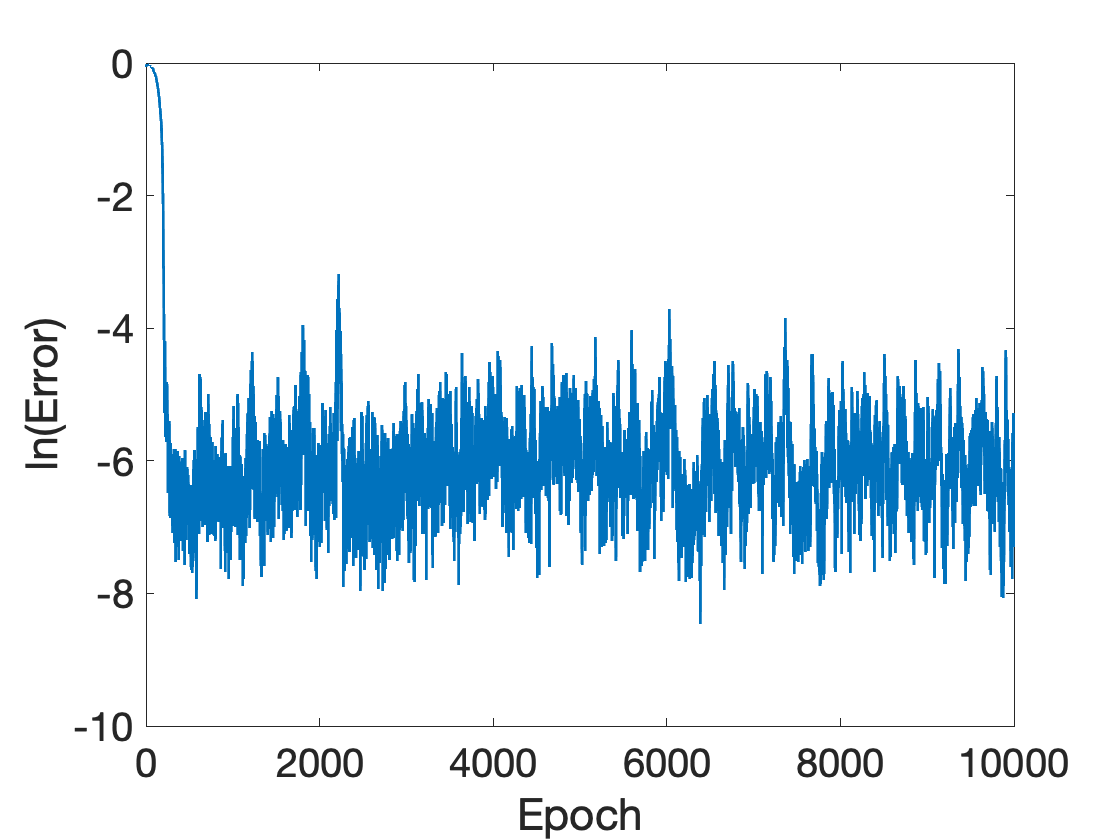
Figure 2: $e^{DL}$ of Example 5.1.

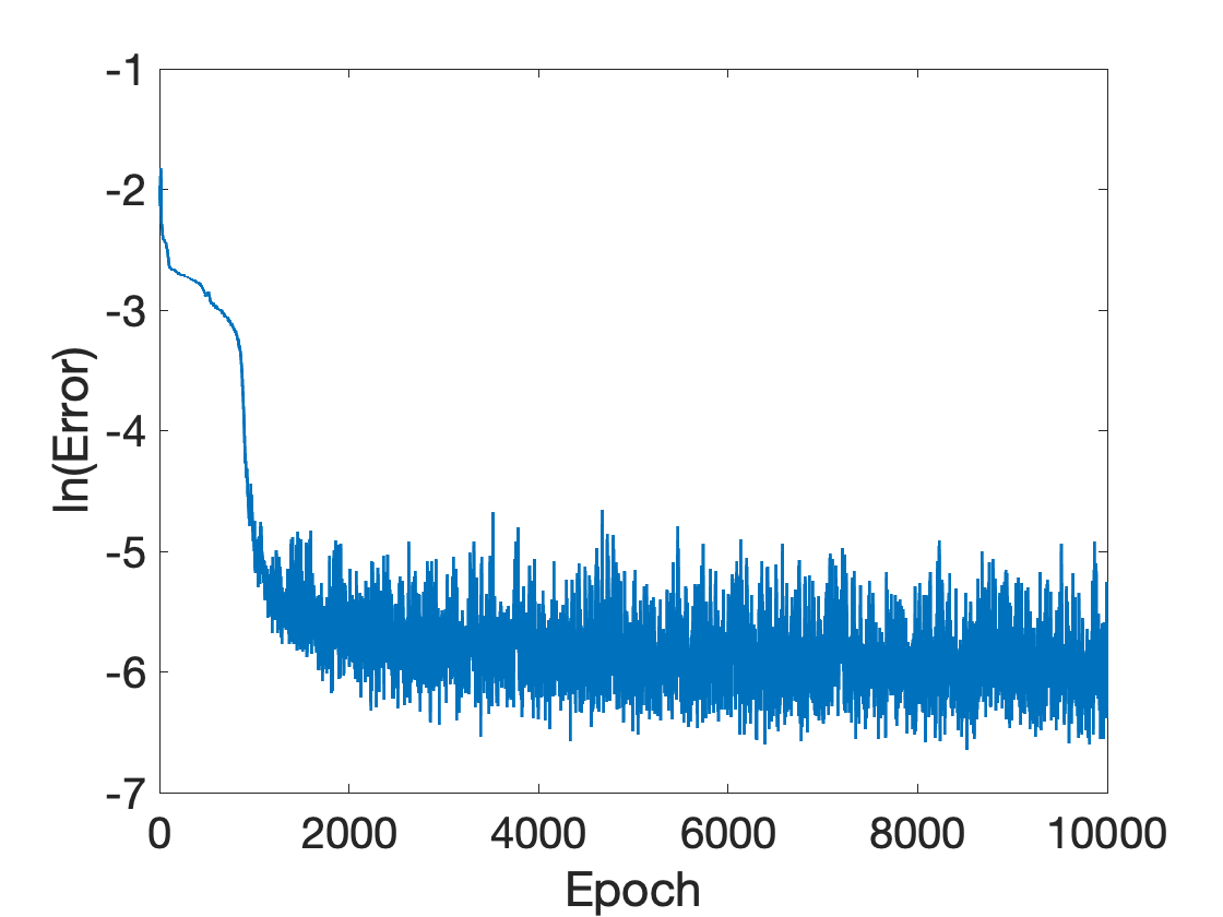
Figure 3: $e^{DL}$ of Example 5.2.

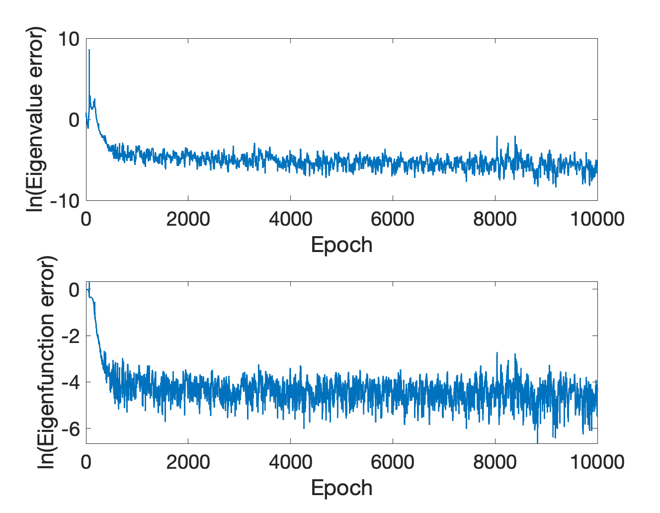
Figure 4: Test errors of Example 5.3.

5.1.2 Variational Inequalities

Example 5.2.

Consider the simplified friction problem

$$\begin{cases}-\Delta u+u=f\quad&\mbox{\rm in}\ \Omega,\\ |\partial_{\bm{n}}u|\leq g,\ u\partial_{\bm{n}}u+g|u|=0\quad&\mbox{\rm on}\ \Gamma_{C},\\ u=0\quad&\mbox{\rm on}\ \Gamma_{D},\end{cases}$$

where $\bm{n}$ is the outer normal vector, $\Omega=(0,1)^{2}$, $\Gamma_{C}=\{1\}\times[0,1]$ and $\Gamma_{D}=\partial\Omega\setminus\Gamma_{C}$. We set $g=1$ and choose $f$ such that the problem has an exact solution $u(x,y)=(\sin x-x\sin 1)\sin(2\pi y)$.

In this experiment, the variational formula in (3.11) with a penalty constant $\gamma=500$ is applied in the deep learning method. To evaluate the test error, we adopt a mesh size $h=\frac{1}{128}$ to generate the uniform triangulation $\mathcal{T}_{h}$ as the test locations. The test errors during training are summarized in Table 4 and Figure 4. From Table 4 and Figure 4, we know the absolute discrete maximum error is reduced to order 1e-3 after 1000 epochs. However, the error oscillates after 2000 epochs and it is difficult to get a highly accurate solution when #Epoch increases.

5.1.3 Eigenvalue Problems

Example 5.3.

Consider the following problem

$$\begin{cases}-u^{\prime\prime}=\lambda u,\quad&x\in\ (0,1),\\ u=0,\quad&x=0\ \mbox{\rm or}\ 1.\end{cases}$$

The smallest eigenvalue is $\pi^{2}$ and the corresponding eigenfunction is $u(x)=\sin(\pi(x-1)).$

In this experiment, the variational formula in (3.15) with $x_{0}=0.5$ and $\gamma=100$ is applied in the deep learning method. To evaluate the test error, we adopt a mesh size $h=\frac{1}{256}$ to generate the uniform triangulation $\mathcal{T}_{h}$ as the test locations. The test errors during training are summarized in Table 4 and Figure 4. From Table 4 and Figure 4, we know the absolute discrete maximum error of the eigenfunction is reduced to order 1e-2 after 300 epochs and the eigenvalue error is reduced to order 1e-3 after 5000 epochs. Both errors oscillate after 1000 epochs and it is hard to to get high-accuracy as #Epoch increases.

5.2 Phase II of Int-Deep: Traditional Iterative Methods

Now we use the approximate solution by deep learning methods as the initial guess in traditional iterative methods. We will show that DNNs of size $O(1)$ and trained with $O(100)$ iterations are good enough for traditional iterative methods to converge in at most $O(\log(\frac{1}{\epsilon}))$ iterations to the $\epsilon$ precision of finite element methods.

5.2.1 Semilinear PDEs

We consider semilinear elliptic equations with homogeneous Dirichlet boundary conditions to demonstrate the efficiency of the Int-Deep framework in Algorithm 1 (deep learning combined with Newton’s method for semilinear PDE) and to verify Theorem 4.1.

Example 5.4.

Consider the following semilinear elliptic equations

$$\begin{cases}-\Delta u-(u-1)^{3}+(u+2)^{2}=f\quad&\mbox{\rm in}\ \Omega,\\ \quad u=0\quad&\mbox{\rm on}\ \partial\Omega,\end{cases}$$

where $\Omega=(0,1)^{d}$ with $d=1$ or $2$. We choose $f$ such that the problem has an exact solution $u(x)=3\sin(2\pi x)$ for $d=1$ and $u(x)=3\sin(2\pi x)\sin(2\pi y)$ for $d=2$.

Case $d=1$.

First of all, we show that Newton’s method cannot converge to a solution without a good initial guess $u_{0}$ and the deep learning method can provide a good initial guess. We apply Newton’s iteration in Algorithm 1 with several types of initial guesses $u_{0}$ listed in Table 5, and the other parameters are taken as $h=\frac{1}{1024}$, $N_{\text{max}}=15$, and $\epsilon=0.01\times h^{2}$. $u^{DL}$ is obtained via the deep learning approach based on the variational formula (3.6) with $\gamma=500$ and $200$ epochs in the Adam. Without good knowledge of the ground truth solution or $u^{DL}$, Newton’s method fails to converge to a good numerical solution.

Table 5: The performance of Newton’s method with different initial guesses $u_{0}$. $\omega$ stands for a Gaussian random noise with mean zero and unit variance.

$u_{0}$	$\#$K	$\|e_{0}^{h}\|_{0,\infty,h}$	$\|e^{h}\|_{0,\infty,h}$	$u_{0}$	$\#$K	$\|e_{0}^{h}\|_{0,\infty,h}$	$\|e^{h}\|_{0,\infty,h}$
${1}$	5	4.00e+0	1.95e+0	$\omega$	6	5.68e+0	3.05e+0
${2}$	5	5.00e+0	1.95e+0	${1}+\omega$	5	6.33e+0	1.95e+0
${5}$	15	8.00e+0	1.28e+5	$-{1}+\omega$	15	6.95e+0	2.65e+6
${-1}$	15	4.00e+0	9.50e+4	$u+\omega$	6	4.03e+0	1.82e-5
${-2}$	12	5.00e+0	4.66e+0	$u+2.5\times\omega$	15	8.89e+0	2.10e+5
${-5}$	15	8.00e+0	6.45e+4	$u^{DL}$	5	2.97e-1	1.82e-5

Besides, we also test the performance of the Picard’s iteration in this example. We apply Picard’s iteration with several types of initial guesses $u_{0}$ listed in Table 6, and the other parameters are taken as $h=\frac{1}{1024}$, $N_{\text{max}}=15$, and $\epsilon=0.01\times h^{2}$. Picard’s iteration fails to converge to the right solution in all tests.

Table 6: The performance of Picard’s method with different initial guesses $u_{0}$. $\omega$ stands for a Gaussian random noise with mean zero and unit variance.

$u_{0}$	$\#$K	$\|e_{0}^{h}\|_{0,\infty,h}$	$\|e^{h}\|_{0,\infty,h}$	$u_{0}$	$\#$K	$\|e_{0}^{h}\|_{0,\infty,h}$	$\|e^{h}\|_{0,\infty,h}$
$\bm{1}$	15	4.00e+0	1.95e+0	$\omega$	15	5.92e+0	1.95e+0
$\bm{0}$	15	3.00e+0	1.95e+0	$u+\omega$	10	3.59e+0	nan

Furthermore, we show that the two-grid method also needs a good initial guess $u_{0}$ for Newton’s method in the coarse grid stage; otherwise, the two-grid method cannot converge well. Denote the mesh size of the coarse grid as $H$ and the mesh size of the fine grid as $h$. The numerical results in Table 7 summarize the performance of the two-grid method with several types of initial guesses $u_{0}$ and different mesh sizes $H$ and $h$. The two grid method can converge to the correct solution only in the case when the initial guess of the coarse grid stage is provided by the deep learning method.

Table 7: The performance of the two-grid method for Example 5.4 in 1D with different initial guesses and mesh sizes.

$u_{0}$	$H$	$h$	$\|e^{h}\|_{0,\infty,h}$	$H$	$h$	$\|e^{h}\|_{0,\infty,h}$	$H$	$h$	$\|e^{h}\|_{0,\infty,h}$
1	$2^{-4}$	$2^{-8}$	1.95e+0	$2^{-5}$	$2^{-10}$	1.95e+0	$2^{-6}$	$2^{-12}$	1.95e+0
-1	$2^{-4}$	$2^{-8}$	2.25e+1	$2^{-5}$	$2^{-10}$	2.74e+2	$2^{-6}$	$2^{-12}$	2.99e+2
0	$2^{-4}$	$2^{-8}$	1.95e+0	$2^{-5}$	$2^{-10}$	1.95e+0	$2^{-6}$	$2^{-12}$	1.95e+0
$\omega$	$2^{-4}$	$2^{-8}$	3.06e+0	$2^{-5}$	$2^{-10}$	3.05e+0	$2^{-6}$	$2^{-12}$	3.05e+0
$u^{DL}$	$2^{-4}$	$2^{-8}$	3.27e-3	$2^{-5}$	$2^{-10}$	1.98e-4	$2^{-6}$	$2^{-12}$	1.23e-5

Next, we show that the initial guess by the deep learning approach enables Newton’s method to converge to a solution with the precision of finite element methods, i.e., the numerical convergence order in terms of $h$ defined by

$$\text{order}:=\log_{2}\frac{\|e_{k}^{h}\|}{\|e_{k}^{h/2}\|}$$

is $2$ as proved by Theorem 4.1, where $\|\cdot\|=\|\cdot\|_{0,\infty,h}$, the same one as used in the above table. This convention applies to other numerical examples. For the purpose of convenience, we choose $h=2^{-\ell}$ for different integers $\ell$’s and let $e_{h^{2}}=h^{2}$ as the theoretical precision of finite element methods. We repeatedly apply the same deep learning method as in Table 5 to generate different initial guesses $u_{0}^{h}$ for different sizes $h$. Let $N_{\text{max}}=15$ and $\epsilon=0.01\times h^{2}$ in Algorithm 1. Table 8 summarizes the performance of Algorithm 1 and numerical results verify the accuracy and the convergence order of the Int-Deep framework, even though the number of epochs in the training of deep learning is $O(100)$ and the initial error is very large.

Table 8: The performance of Int-Deep in Algorithm 1 for Example 5.4 in 1D with different mesh sizes $h$.

$h$	$e_{h^{2}}$	$\#$ Epoch	$\|e^{DL}\|_{0,\infty,h}$	$\#$K	$\|e^{h}\|_{0,\infty,h}$	order
$2^{-7}$	6.10e-5	200	2.97e-1	5	1.17e-3	-
$2^{-8}$	1.53e-5	200	2.97e-1	5	2.92e-4	2.00
$2^{-9}$	3.81e-6	200	2.97e-1	5	7.29e-5	2.00
$2^{-10}$	9.54e-7	200	2.97e-1	5	1.82e-5	2.00
$2^{-11}$	2.38e-7	200	2.97e-1	5	4.56e-6	2.00
$2^{-12}$	5.96e-8	200	2.97e-1	5	1.14e-6	2.00
$2^{-13}$	1.49e-8	200	2.97e-1	5	2.85e-7	2.00
$2^{-14}$	3.73e-9	200	2.97e-1	5	7.12e-8	2.00

Finally, we show that the performance of the Int-Deep in Algorithm 1 is independent of the size of DNNs, which is supported by the numerical results in Table 9.

Table 9: The performance of Int-Deep in Algorithm 1 for Example 5.4 in 1D with different DNN width $N$ and depth $L$ when $h=\frac{1}{1024}$ and $\#$Epoch = 400.

	10			30			50
	${\|e^{DL}\|_{0,\infty,h}}$	$\|e^{h}\|_{0,\infty,h}$	$\#$K	${\|e^{DL}\|_{0,\infty,h}}$	$\|e^{h}\|_{0,\infty,h}$	$\#$K	${\|e^{DL}\|_{0,\infty,h}}$	$\|e^{h}\|_{0,\infty,h}$	$\#$K
2	3.72e+0	1.82e-5	8	2.27e-1	1.82e-5	5	5.19e-2	1.82e-5	4
4	1.05e-1	1.82e-5	4	1.63e-2	1.82e-5	3	1.51e-2	1.82e-5	3
6	9.84e-2	1.82e-5	4	8.48e-3	1.82e-5	3	5.34e-3	1.82e-5	3

Case $d=2$.

Again, we show that the initial guess by the deep learning approach enables Newton’s method to converge to a solution with the precision of finite element methods, i.e., the numerical convergence order in terms of $h$ is almost $2$ as proved by Theorem 4.1. We repeatedly apply the variational formula in (3.6) with $\gamma=500$ and the deep learning method to generate different initial guesses $u_{0}^{h}$ for different sizes $h$. Let $N_{\text{max}}=15$ and $\epsilon=0.01\times h^{2}$ in Algorithm 1. Let $e_{h^{2}}=|h^{2}\log h|$. Table 10 summarizes the performance of Algorithm 1 and numerical results verify the accuracy and the convergence order of the Int-Deep framework, even though the number of epochs in deep learning is $O(100)$ and the initial error is very large.

Table 10: The performance of Int-Deep in Algorithm 1 for Example 5.4 in 2D with different mesh sizes $h$.

$h$	$e_{h^{2}}$	$\#$ Epoch	$\|e^{DL}\|_{0,\infty,h}$	$\#$K	$\|e^{h}\|_{0,\infty,h}$	order
$2^{-4}$	1.08e-2	200	2.19e+0	5	2.03e-1	-
$2^{-5}$	3.38e-3	200	2.19e+0	5	5.92e-2	1.78
$2^{-6}$	1.02e-3	200	2.20e+0	5	1.55e-2	1.94
$2^{-7}$	2.96e-4	200	2.20e+0	6	3.92e-3	1.98
$2^{-8}$	8.46e-5	200	2.20e+0	6	9.83e-4	2.00

Finally, we show that the performance of the Int-Deep in Algorithm 1 is independent of the size of DNNs, which is supported by the numerical results in Table 11.

Table 11: The performance of Int-Deep in Algorithm 1 for Example 5.4 in 2D with different DNN width $N$ and depth $L$ when $h=\frac{1}{128}$ and $\#$Epoch = 400.

	10			30			50
	${\|e^{DL}\|_{0,\infty,h}}$	$\|e^{h}\|_{0,\infty,h}$	$\#$K	${\|e^{DL}\|_{0,\infty,h}}$	$\|e^{h}\|_{0,\infty,h}$	$\#$K	${\|e^{DL}\|_{0,\infty,h}}$	$\|e^{h}\|_{0,\infty,h}$	$\#$K
2	3.15e+0	3.92e-3	6	2.91e+0	3.92e-3	6	3.32e+0	3.92e-3	6
4	4.06e+0	3.92e-3	6	2.53e+0	3.92e-3	5	7.59e-1	3.92e-3	4
6	3.54e+0	3.92e-3	6	1.20e+0	3.92e-3	4	1.05e+0	3.92e-3	4

5.2.2 Linear eigenvalue problems

Here, we demonstrate the efficiency of the Int-Deep framework in Algorithm 2 (deep learning combined with the power method) and verify Theorem 4.2.

Example 5.5.

Consider the following problem

$$\begin{cases}-\Delta u=\lambda u\quad&\mbox{\rm in}\ \Omega,\\ \quad u=0\quad&\mbox{\rm on}\ \partial\Omega,\end{cases}$$

where $\Omega=(0,1)^{d}$ for $d=1$ and $2$. The smallest eigenvalue is $d\pi^{2}$. The corresponding eigenfunction is $u(x)=\sin(\pi(x-1))$ for $d=1$, and $u(x,y)=\sin(\pi(x-1))\sin(\pi(y-1))$ for $d=2$.

Case $d=1$.

We show that the initial guess by the deep learning approach enables the power method to quickly converge to a solution with the precision of finite element methods, i.e., the numerical convergence order in terms of $h$ is $2$ as proved by Theorem 4.2. We repeatedly apply the variational formula in (3.15) (with $x_{0}=0.5$ and $\gamma=100$) and the deep learning method to generate different initial guesses $u_{0}^{h}$ for different sizes $h$. Let $N_{\text{max}}=10$ and $\epsilon=h^{2}$ in Algorithm 2. Table 12 summarizes the performance of Algorithm 2 and numerical results verify the accuracy and the convergence order of the Int-Deep framework, even though the number of epochs in deep learning is $O(100)$.

Table 12: The performance of Int-Deep in Algorithm 2 for Example 5.5 in 1D with different mesh sizes $h$.

$h$	$\#$Epoch	$\|e^{h}_{0}\|_{0}$	$\#$K	$|\lambda-\lambda^{h}|$	eigenvalue order	$\|e^{h}\|_{0}$	eigenfunction order
$2^{-5}$	300	1.13e-2	3	7.93e-3	-	8.08e-4	-
$2^{-6}$	300	1.14e-2	4	1.98e-3	2.00	2.02e-4	2.00
$2^{-7}$	300	1.14e-2	5	4.95e-4	2.00	5.05e-5	2.00
$2^{-8}$	300	1.14e-2	6	1.24e-4	2.00	1.26e-5	2.00
$2^{-9}$	300	1.14e-2	7	3.04e-5	2.03	3.17e-6	2.00

Next, we show that the performance of Int-Deep in Algorithm 2 is independent of the size of DNNs, which is supported by the numerical results in Table 13.

Table 13: The performance of Int-Deep in Algorithm 2 for Example 5.5 in 1D with different DNN width $N$ and depth $L$ when $h=\frac{1}{512}$ and $\#$Epoch = 400.

	10			30			50
	$|\lambda-\lambda^{h}|$	$\|e^{h}\|_{0}$	$\#$K	$|\lambda-\lambda^{h}|$	$\|e^{h}\|_{0}$	$\#$K	$|\lambda-\lambda^{h}|$	$\|e^{h}\|_{0}$	$\#$K
2	3.06e-5	3.30e-6	7	2.61e-5	3.40e-6	8	3.67e-5	3.47e-6	8
4	3.10e-5	3.26e-6	6	3.09e-5	3.17e-6	6	3.24e-5	3.19e-6	8
6	4.25e-5	4.42e-6	8	2.98e-5	3.24e-6	7	3.09e-5	3.30e-6	6

Case $d=2$.

Again, we show that the initial guess by the deep learning approach enables the power method to quickly converge to a solution with the precision of finite element methods, i.e., the numerical convergence order in terms of $h$ is $2$ as proved by Theorem 4.2. We repeatedly apply the variational formula in (3.15) (with $\bm{x}_{0}=(0.5,0.5)$ and $\gamma=100$) and the deep learning method to generate different initial guesses $u_{0}^{h}$ for different sizes $h$. Let $N_{\text{max}}=10$ and $\epsilon=h^{2}$ in Algorithm 2. Table 14 summarizes the performance of Algorithm 2 and numerical results verify the accuracy and the convergence order of the Int-Deep framework, even though the number of epochs in deep learning is $O(100)$.

Table 14: The performance of Int-Deep in Algorithm 2 for Example 5.5 in 2D with different mesh sizes $h$.

$h$	#Epoch	$\|e^{h}_{0}\|_{0}$	#K	$|\lambda-\lambda^{h}|$	eigenvalue order	$\|e^{h}\|_{0}$	eigenfunction order
$2^{-4}$	300	5.56e-2	4	1.91e-1	-	6.63e-3	-
$2^{-5}$	300	5.65e-2	5	4.76e-2	2.00	1.70e-3	1.96
$2^{-6}$	300	5.68e-2	7	1.19e-2	2.00	4.19e-4	2.02
$2^{-7}$	300	5.69e-2	8	2.97e-3	2.00	1.07e-4	1.97
$2^{-8}$	300	5.69e-2	10	7.43e-4	2.00	2.62e-5	2.03

Next, we show that the performance of Int-Deep in Algorithm 2 is independent of the size of DNNs, which is supported by the numerical results in Table 15.

Table 15: The performance of Int-Deep in Algorithm 2 for Example 5.5 in 2D with different DNN width $N$ and depth $L$ when $h=\frac{1}{128}$ and $\#$Epoch = 400.

	10			30			50
	$|\lambda-\lambda^{h}|$	$\|e^{h}\|_{0}$	$\#$K	$|\lambda-\lambda^{h}|$	$\|e^{h}\|_{0}$	$\#$K	$|\lambda-\lambda^{h}|$	$\|e^{h}\|_{0}$	$\#$K
2	2.97e-3	1.09e-4	9	2.97e-3	1.08e-4	8	2.97e-3	1.08e-4	8
4	2.97e-3	1.07e-4	7	2.97e-3	1.07e-4	7	2.97e-3	1.09e-4	7
6	2.97e-3	1.07e-4	6	2.97e-3	1.11e-4	7	2.97e-3	1.05e-4	8

5.2.3 Nonlinear eigenvalue problems

As used in [24], denote by $res^{DL}$ and $res^{h}$ the residuals of $u^{DL}$ and $u^{h}$ corresponding to the matrix form of (4.11), respectively. In this example, we denote $\|\cdot\|_{2}$ as the vector $L_{2}-$norm in Euclidian space. Then we investigate the accuracy of Int-Deep framework in Algorithm 3 through the case of the nonlinear Schrödinger equation.

Example 5.6.

Consider the following problem

$$\begin{cases}-\Delta u+V(x)u+10u^{3}=\lambda u&\quad\mbox{\rm in}\ \Omega,\\ u=0&\quad\mbox{\rm on}\ \partial\Omega,\\ \|u\|_{0}=1,\end{cases}$$

where $\Omega=(0,1)^{d}$ for $d=1,2$, $V(x)$ is a potential with two Gaussian wells on $(0,1)$ for $d=1$, and with four Gaussian wells on $(0,1)^{2}$ for $d=2$.

Case $d=1$

We first show that the initial guess by the deep learning approach enables Newton’s method to quickly converge to the target solution. We repeatedly apply the variational formula in (3.19) (with $x_{0}=0.5$ and $\gamma=100$) and the deep learning method to generate different initial guesses $u_{0}^{h}$ for different sizes $h$. Let $N_{\text{max}}=10$ and $\epsilon=h^{2}$ in Algorithm 3. Table 16 summarizes the performance of Algorithm 3.

Table 16: The performance of Int-Deep in Algorithm 3 for Example 5.6 in 1D with different mesh sizes $h$.

$h$	$\#$Epoch	${\|res^{DL}\|_{2}}$	$\lambda^{DL}$	$\#$K	${\|res^{h}\|_{2}}$	$\lambda^{h}$
$2^{-5}$	300	6.10e-1	23.71	2	2.41e-6	23.60
$2^{-6}$	300	4.72e-1	23.69	3	1.13e-10	23.58
$2^{-7}$	300	3.46e-1	23.69	3	1.54e-11	23.58
$2^{-8}$	300	2.49e-1	23.69	3	2.57e-12	23.58
$2^{-9}$	300	1.77e-1	23.69	3	1.51e-12	23.58

Next, we show that the performance of Int-Deep in Algorithm 3 is independent of the size of DNNs, which is supported by the numerical results in Table 17.

Table 17: The performance of Int-Deep in Algorithm 3 for Example 5.6 in 1D with different DNN width $N$ and depth $L$ when $h=\frac{1}{512}$ and $\#$Epoch = 400.

	10			30			50
	$\lambda^{h}$	${\|res^{h}\|_{2}}$	$\#$K	$\lambda^{h}$	${\|res^{h}\|_{2}}$	$\#$K	$\lambda^{h}$	${\|res^{h}\|_{2}}$	$\#$K
2	23.58	1.33e-12	5	23.58	1.44e-12	4	23.58	1.50e-12	3
4	23.58	1.53e-12	3	23.58	2.14e-12	3	23.58	1.48e-12	3
6	23.58	1.44e-12	3	23.58	1.49e-12	3	23.58	1.34e-12	3

Case $d=2$.

Again, we show that the initial guess by the deep learning approach enables Newton’s method to quickly converge to the target solution. We repeatedly apply the variational formula in (3.19) (with $\bm{x}_{0}=(0.5,0.5)$ and $\gamma=100$) and the deep learning method to generate different initial guesses $u_{0}^{h}$ for different sizes $h$. Let $N_{\text{max}}=10$ and $\epsilon=h^{2}$ in Algorithm 3. Table 18 summarizes the performance of Algorithm 3.

Table 18: The performance of Int-Deep in Algorithm 3 for Example 5.6 in 2D with different mesh sizes $h$.

$h$	$\#$Epoch	${\|res^{DL}\|_{2}}$	$\lambda^{DL}$	$\#$K	${\|res^{h}\|_{2}}$	$\lambda^{h}$
$2^{-4}$	300	4.07e-1	39.74	2	9.06e-6	39.46
$2^{-5}$	300	2.46e-1	39.49	2	2.13e-6	39.19
$2^{-6}$	300	1.35e-1	39.43	3	1.43e-10	39.12
$2^{-7}$	300	7.04e-2	39.42	3	1.53e-11	39.10

Next, we show that the performance of Int-Deep in Algorithm 3 is independent of the size of DNNs, which is supported by the numerical results in Table 19.

Table 19: The performance of Int-Deep in Algorithm 3 for Example 5.6 in 2D with different DNN width $N$ and depth $L$ when $h=\frac{1}{128}$ and $\#$Epoch = 400.

	10			30			50
	$\lambda^{h}$	${\|res^{h}\|_{2}}$	$\#$K	$\lambda^{h}$	${\|res^{h}\|_{2}}$	$\#$K	$\lambda^{h}$	${\|res^{h}\|_{2}}$	$\#$K
2	39.10	1.60e-12	3	39.10	7.88e-13	4	39.10	4.26e-13	3
4	39.10	3.28e-10	3	39.10	1.30e-11	3	39.10	6.33e-12	3
6	39.10	3.77e-11	3	39.10	8.30e-11	3	39.10	2.10e-10	3

6 Conclusion

This paper proposed the Int-Deep framework from a new point of view for designing highly efficient solvers of low-dimensional nonlinear PDEs with a finite element accuracy leveraging both the advantages of traditional algorithms and deep learning approaches. The Int-Deep framework consists of two phases. In the first phase, an approximate solution to the given nonlinear PDE is obtained via deep learning approaches using DNNs of size $O(1)$ and $O(100)$ iterations. In the second phase, the approximate solution provided by deep learning can serve as a good initial guess such that traditional iterative methods converge in $O(\log(\frac{1}{\epsilon}))$ iterations to the $\epsilon$ precision of finite element methods. The Int-Deep framework outperforms existing purely deep learning-based methods or traditional iterative methods. The code can be shared per request.

In particular, based on variational principles, we propose new methods to formulate the problem of solving nonlinear PDEs into an unconstrained minimization problem of an expectation over a function space parametrized via DNNs, which can be solved efficiently via batch stochastic gradient descent (SGD) methods due to the special form of expectation. Unlike previous methods in which the form of expectation is only derived for nonlinear PDEs related to variational equations, our proposed method can also handle variational inequalities and eigenvalue problems, providing a unified variational framework for a wider range of nonlinear problems. With the good initialization given by deep learning, we hope to reduce the difficulty of designing an efficient traditional iterative algorithm for variational inequalities. We will leave this as future work.

Acknowledgments. J. H. was partially supported by NSFC (Grant No.11571237). H. Y. was partially supported by the National Science Foundation under the grant award 1945029. We would like to thank reviewers for their valuable comments to improve the manuscript.

Appendix

Appendix A Proof of Theorem 4.1

Making use of the assumption A2 in Section 4.1, we immediately have the following result (see [58]).

Lemma A.1.

Let $u\in W^{2,\infty}(\Omega)$ be a solution of (4.1). There exist two positive constant $C_{1}^{u}$ and $C_{2}^{u}$ such that if a function $v$ satisfies that $\|v-u\|_{0,\infty}\leq C_{1}^{u}$, then

$$C_{2}^{u}\|\phi\|_{1}\leq\sup_{\chi\in V}\frac{a_{v}(\phi,\chi)}{\|\chi\|_{1}},\quad\phi\in V.$$

The mathematical analysis for the finite element method (4.5) is very technical and has been established in [59]. In the following two lemmas, we collect some results which will be used frequently later on.

Lemma A.2.

Let $u\in W^{2,\infty}(\Omega)$ be a solution of (4.2). Then there exists a constant $h_{0}>0$ and a positive constant $C_{3}^{u}$ independent of $h$ such that if $h<h_{0}$ and a function $v$ satisfies $\|v-u\|_{0,\infty}\leq C_{1}^{u}$, then

$$C_{3}^{u}\|\phi\|_{1}\leq\sup_{\chi\in V_{h}}\frac{a_{v}(\phi,\chi)}{\|\chi\|_{1}},\quad\phi\in V_{h}.$$

This lemma can be derived by using Lemma A.1 and the arguments for proving Lemma 2.2 in [59].

Lemma A.3.

Let $u\in W^{2,\infty}(\Omega)$ be a solution of (4.2). Then there exists a positive constant $h_{1}<h_{0}$ such that if $h<h_{1}$, the finite element method (4.5) has exactly one solution $u^{h}$ satisfying

$$\|u-u^{h}\|_{1}\leq C_{4}^{u}$$

for a positive constant $C_{4}^{u}$ independent of $h$. Moreover,

$$\lim_{h\to 0^{+}}\|u-u^{h}\|_{1}=0.$$

Lemma A.4.

Let $u\in W^{2,\infty}(\Omega)$ be a solution of (4.2) and $u^{h}$ be the finite element method of (4.5). Then, there exists a positive constant $h_{2}<h_{1}$ such that if $h<h_{2}$,

$$\|u-u^{h}\|_{0,\infty}\lesssim h^{2}\quad\quad\quad\quad\,\,when\ d=1,$$

$$\|u-u^{h}\|_{0,\infty}\lesssim h^{2}|\log(h)|\quad when\ d=2.$$

Proof.

The estimate for $d=2$ is given in [59]. We will derive the estimate for $d=1$ following some ideas in [59]. To this end, we first introduce an elliptic projection operator $P_{h}$ such that if $u\in V$, then $P_{h}u\in V_{h}$ satisfies

$$(\nabla(P_{h}u),\nabla\chi)=(\nabla u,\nabla\chi),\quad\chi\in V_{h}.$$ (A.1)

It is shown in [66] that

$$\|u-P_{h}u\|_{0,\infty}\lesssim\|u-P_{h}u\|_{1}\lesssim h^{2}|u|_{2,\infty}.$$ (A.2)

On the other hand, the finite element solution $u^{h}$ satisfies

$$(\nabla u^{h},\nabla\chi)+(f(u^{h}),\chi)=0,\quad\chi\in V_{h}.$$

Recalling the relation (A.1) and using (4.2) gives

$$(\nabla(P_{h}u),\nabla\chi)=(\nabla u,\nabla\chi)=-(f(u),\chi),\quad\chi\in V_{h}.$$

Hence, subtracting the last two equations and using Taylor’s expansion yield

$$a_{P_{h}u}((u^{h}-P_{h}u),\chi)=-\frac{1}{2}(f^{\prime\prime}(\zeta)(u^{h}-P_{h}u)^{2},\chi)-(f(P_{h}u)-f(u),\chi),\quad\chi\in V_{h},$$

where $\zeta=\nu(x)u^{h}(x)+(1-\nu(x))(P_{h}u)(x)$ for some $\nu(x)\in(0,1)$. We have by the estimate (A.2) that there exists a positive constant $\bar{h}<h_{1}$ such that if $h<\bar{h}$, $\|P_{h}u-u\|_{0,\infty}\leq C_{1}^{u}$. In this case, it follows from Lemma A.2 and the last equation that

$$\|u^{h}-P_{h}u\|_{1} \lesssim\sup_{\chi\in V_{h}}\frac{a_{P_{h}u}((u^{h}-P_{h}u),\chi)}{\|\chi\|_{1}}$$

$$\lesssim\|u^{h}-P_{h}u\|^{2}_{0,\infty}+\|f(u)-f(P_{h}u)\|_{0,\infty}$$

$$\lesssim\|u^{h}-P_{h}u\|^{2}_{1}+\|u-P_{h}u\|_{0,\infty}$$

$$\leq C\|u^{h}-P_{h}u\|_{1}^{2}+C\|u-P_{h}u\|_{0,\infty},$$ (A.3)

where $C>0$ is a generic constant. On the other hand, it follows from Lemma A.3 and the estimate (A.2) that

$$\|u^{h}-P_{h}u\|_{1}\leq\|u-u^{h}\|_{1}+\|u-P_{h}u\|_{1}\to 0\quad\mbox{ as }h\to 0^{+}.$$

Hence, there exists a positive constant $h_{2}<\bar{h}$ such that if $h<h_{2}$, then $C\|u^{h}-P_{h}u\|_{1}<1/2$, which combined with (A.3) readily implies

$$\|u^{h}-P_{h}u\|_{1}\lesssim\|u-P_{h}u\|_{0,\infty}.$$

Therefore, by the Sobolev embedding theorem and the estimate (A.2),

$$\|u-u^{h}\|_{0,\infty} \leq\|u-P_{h}u\|_{0,\infty}+\|P_{h}u-u^{h}\|_{0,\infty}$$

$$\lesssim\|u-P_{h}u\|_{0,\infty}+\|P_{h}u-u^{h}\|_{1}\lesssim\|u-P_{h}u\|_{0,\infty}\lesssim h^{2}|u|_{2,\infty},$$

as required. ∎

Remark 1.

As shown in [11], we require to make certain strong regularity assumption on the solution to problem (4.2) for $d=3$, so as to derive the maximum norm estimate for the related finite element method. To avoid too technical treatment, we skip the further discussion in this case.

The following result plays an important role in the convergence analysis of Int-Deep for solving the finite element method (4.5), which will be introduced later on.

Lemma A.5.

Let $u\in W^{2,\infty}(\Omega)$ be a solution of (4.2). Let $u^{h}$ be an approximation of $u$ obtained by the finite element method (4.5). Assume that $h<h_{2}$ with $h_{2}$ the same as given in Lemma A.4. For any $v\in V_{h}\cap B(u)$, define a mapping $Tv=v+w$, where $w\in V_{h}$ is uniquely determined by

$$(\nabla w,\nabla\chi)+(f^{\prime}(v)w,\chi)=-(\nabla v,\nabla\chi)-(f(v),\chi),\quad\chi\in V_{h}.$$ (A.4)

Then there holds

$$\|u^{h}-Tv\|_{1}\lesssim\|u^{h}-v\|_{0,p}^{2}\lesssim\|u^{h}-v\|_{1}^{2}.$$

Proof.

Recalling the definition (4.5), we know

$$(\nabla u^{h},\nabla\chi)+(f(u^{h}),\chi)=0,\quad\chi\in V_{h},$$

Subtracting the above equation from (A.4) and reorganizing terms, we find

$$(\nabla E_{h},\nabla\chi)+(f(u^{h})-f(v)-f^{\prime}(v)w,\chi)=0,\quad\chi\in V_{h},$$

where $E_{h}=u^{h}-Tv$. Furthermore, use Taylor’s expansion to get

$$a_{v}(E_{h},\chi)=-\frac{1}{2}(f^{\prime\prime}(\zeta)(u^{h}-v)^{2},\chi),\quad\chi\in V_{h},$$

where $\zeta=(1-\nu(x))v(x)+\nu(x)u^{h}(x)$ with $\nu(x)\in(0,1)$. Since $h<h_{2}$ and $v\in B(u)$, from Lemma A.3 it follows that $\|\zeta\|_{0,\infty}$ is uniformly bounded with respect to $h$. Hence, by the H$\ddot{\text{o}}$lder inequality and the Sobolev embedding theorem, for $p>2$ and any $\chi\in V_{h}$,

$$a_{v}(E_{h},\chi) \lesssim\int_{\Omega}(u^{h}-v)^{2}|\chi|\,{\rm d}x$$

$$\lesssim\|(u^{h}-v)^{2}\|_{0,p/2}\|\chi\|_{0,p/p-2}\lesssim\|u^{h}-v\|_{0,p}^{2}\|\chi\|_{1},$$

where the generic constant is independent of $h$ but depends on $p$. The combination of the last estimate with Lemma A.2 immediately implies

$$\|E_{h}\|_{1}\lesssim\|u^{h}-v\|_{0,p}^{2}\lesssim\|u^{h}-v\|_{1}^{2},$$

as required. ∎

Now we are ready to prove Theorem 4.1.

Proof.

Denote $E_{k}^{h}=u^{h}-u_{k}^{h}$. Applying Lemma A.5 gives rise to

$$\|E_{k+1}^{h}\|_{1}\lesssim\|E_{k}^{h}\|_{0,p}^{2}\lesssim\|E_{k}^{h}\|_{1}^{2}.$$ (A.5)

When $d=1$, By the Sobolev embedding theorem and (A.5),

$$\|E_{k+1}^{h}\|_{0,\infty}\lesssim\|E_{k+1}^{h}\|_{1}\lesssim\|E_{k}^{h}\|_{0,p}^{2}\lesssim\|E_{k}^{h}\|_{0,\infty}^{2}.$$

This means there exists a positive constant $c_{1}$ such that $\|E_{k}^{h}\|_{0,\infty}\leq c_{1}\|E_{k-1}^{h}\|_{0,\infty}^{2}$. Hence,

$$c_{1}\|E_{k}^{h}\|_{0,\infty}\leq(c_{1}\|E_{k-1}^{h}\|_{0,\infty})^{2}\leq(c_{1}\|E_{0}^{h}\|_{0,\infty})^{2^{k}}.$$

On the other hand, it follows from Lemma A.4 and error estimates for the interpolation operator $I_{h}$ (cf. [11, 16]) that

$$\|E_{0}^{h}\|_{0,\infty} =\|u^{h}-u_{0}^{h}\|_{0,\infty}$$

$$\leq\|u^{h}-u\|_{0,\infty}+\|u-I_{h}u\|_{0,\infty}+\|I_{h}u-I_{h}u^{DL}\|_{0,\infty}$$

$$\leq c_{0}(h^{2}+\delta),$$

where $c_{0}>0$ is a generic constant. Let $\beta_{1}=c_{1}c_{0}(h^{2}+\delta)$. Then

$$\|E_{k}^{h}\|_{0,\infty}\leq\beta_{1}^{2^{k}}/c_{1}.$$ (A.6)

When $d=2$, for any given number $p>2$, we have by the Sobolev embedding theorem and (A.5) that

$$\|E_{k+1}^{h}\|_{0,p}\lesssim\|E_{k+1}^{h}\|_{1}^{2}\lesssim\|E_{k}^{h}\|_{0,p}^{2},$$

which implies $c_{2}\|E_{k}^{h}\|_{0,p}\leq(c_{2}\|E_{0}^{h}\|_{0,p})^{2^{k}}$ for a generic positive constant $c_{2}$. In addition, by Lemma A.4 and error estimates for $I_{h}$,

$$\|E_{0}^{h}\|_{0,p} =\|u^{h}-u_{0}^{h}\|_{0,p}$$

$$\leq\|u^{h}-u\|_{0,p}+\|u-I_{h}u\|_{0,p}+\|I_{h}u-u_{0}^{h}\|_{0,p}$$

$$\lesssim\|u^{h}-u\|_{0,\infty}+\|u-I_{h}u\|_{0,\infty}+\|I_{h}u-u_{0}^{h}\|_{0,\infty}$$

$$\leq c_{3}(h^{2}|\log h|+\delta),$$

where $c_{3}>0$ is a generic constant independent of $h$ and $\delta$ but depending on $p$. Let $\beta_{2}=c_{2}c_{3}(h^{2}|\log h|+\delta)$. Then

$$\|E_{k}^{h}\|_{0,p}\leq\beta_{2}^{2^{k}}/c_{2},$$

and further by the inverse inequality for finite elements,

$$\|E_{k}^{h}\|_{0,\infty}\lesssim h^{-2/p}\|E_{k}^{h}\|_{0,p}\lesssim h^{-2/p}\beta_{2}^{2^{k}}.$$ (A.7)

Now, we have by (A.6), (A.7) and Lemma A.4 that

$$\|u-u_{k}^{h}\|_{0,\infty}\leq\|u-u^{h}\|_{0,\infty}+\|u^{h}-u_{k}^{h}\|_{0,\infty}\lesssim h^{2}+\beta_{1}^{2^{k}}\quad\mbox{for }d=1,$$

and

$$\|u-u_{k}^{h}\|_{0,\infty}\leq\|u-u^{h}\|_{0,\infty}+\|u^{h}-u_{k}^{h}\|_{0,\infty}\lesssim h^{2}|\log h|+h^{-2/p}\beta_{2}^{2^{k}}\quad\mbox{for }d=2.$$

The proof is complete.

∎

Appendix B Proof of Theorem 4.2

The proof of Theorem 4.2 is rather involved and requires the following elementary but nontrivial result as a key bridge to produce the optimal convergence analysis.

Lemma B.1.

Let $\{a_{k}\}$ be a sequence satisfying $a_{k+1}\leq a_{k}^{2}+b$ for $k=0,1,2,\cdots$. If $0\leq a_{0}<1/2$ and $0<b<1/4$, then

$$a_{k}\leq a_{0}^{2^{k}}+\left(2+\frac{1}{1-2a_{0}}\right)b.$$ (B.1)

Proof.

First of all, construct an auxiliary sequence $\{A_{k}\}$ generated by

$$A_{k+1}=A_{k}^{2}+b,\quad k=0,1,2,\cdots;\quad A_{0}=a_{0}.$$ (B.2)

It is easy to check $a_{k}\leq A_{k}$ for all nonnegative integer $k$. The recursive relation (B.2) is a fixed point iteration corresponding to the following fixed point equation

$$A=A^{2}+b\Rightarrow A^{2}-A+b=0,$$ (B.3)

which has exactly two fixed points

$$\alpha_{0}=\frac{2b}{1+\sqrt{1-4b}}\quad\mbox{and}\quad\alpha_{1}=\frac{1+\sqrt{1-4b}}{2}.$$

Next, let us study the boundedness of the sequence $\{A_{k}\}$. When $A_{0}\leq\alpha_{0}$, we have by mathematical induction that $A_{k}\leq\alpha_{0}$ for $k=0,1,2,\cdots$. In fact, if $k=0$ the statement is true. Now we assume it holds for $k=m$ with $m$ an any given natural number, i.e. $A_{m}\leq\alpha_{0}$. Then, observing that $\alpha_{0}$ satisfies the equation (B.3), we immediately know

$$A_{m+1}=A_{m}^{2}+b\leq\alpha_{0}^{2}+b=\alpha_{0}.$$

So the statement is really true by the principle of mathematical induction. On the other hand, it is easy to check by a direct computation that $\alpha_{0}\leq 2b$. Hence, if $A_{0}\leq\alpha_{0}$, there holds

$$a_{k}\leq A_{k}\leq\alpha_{0}\leq 2b.$$ (B.4)

When $\alpha_{0}\leq A_{0}\leq\alpha_{1}$, we use mathematical induction again to know $\alpha_{0}\leq A_{k}\leq\alpha_{1}$ for any nonnegative integer $k$. Let us now consider a function $f(x)$ defined by

$$f(x)=x+\frac{b}{x},\quad x\in[\alpha_{0},\alpha_{1}].$$

Clearly, it is convex over $[\alpha_{0},\alpha_{1}]$ and hence must take the maximum value over the interval at one of the two end points. However, recalling the definitions of $\alpha_{0}$ and $\alpha_{1}$, we easily know

$$f(\alpha_{0})=f(\alpha_{1})=1,$$

which implies $f(x)\leq 1$ for $x\in[\alpha_{0},\alpha_{1}]$. Thus, since $A_{k}\in[\alpha_{0},\alpha_{1}]$, we find

$$\frac{A_{k+1}}{A_{k}}=\frac{A_{k}^{2}+b}{A_{k}}=f(A_{k})\leq 1;$$

in other words, $\{A_{k}\}$ is a decreasing sequence. Therefore, the result $A_{k}\leq a_{0}$ also holds in this case. To sum up, we find that if $a_{0}<1/2<\alpha_{1}$, $A_{k}\leq a_{0}$ for all nonnegative integer $k$.

To further our analysis, we require to construct another auxiliary sequence generated by

$$B_{k+1}=B_{k}^{2},\quad k=0,1,2,\cdots;\quad B_{0}=a_{0}.$$ (B.5)

It is evident that $B_{k}=B_{0}^{2^{k}}=a_{0}^{2^{k}}$ and $B_{k}\leq A_{k}$. Denote $d_{k}=A_{k}-B_{k}\geq 0$. Recalling the definitions (B.2) and (B.5), and using the fact that $A_{k}\leq a_{0}$ obtained above, we find

$$d_{k+1}=A_{k}^{2}+b-B_{k}^{2}=d_{k}(A_{k}+B_{k})+b\leq 2a_{0}d_{k}+b,$$

which readily yields

$$d_{k}\leq(2a_{0})^{k}d_{0}+\frac{1-(2a_{0})^{k}}{1-2a_{0}}b\leq\frac{1}{1-2a_{0}}b$$

by noting that $d_{0}=0$. Therefore,

$$A_{k}=B_{k}+d_{k}\leq B_{0}^{2^{k}}+\frac{1-(2a_{0})^{k}}{1-2a_{0}}b=a_{0}^{2^{k}}+\frac{1-(2a_{0})^{k}}{1-2a_{0}}b$$

and

$$a_{k}\leq A_{k}\leq a_{0}^{2^{k}}+\frac{1}{1-2a_{0}}b.$$ (B.6)

We then obtain the required estimate by combining (B.4) and (B.6). ∎

Now we are ready to present the proof of Theorem 4.2.

Proof.

For any $\phi\in V_{h}$, we know

$$a(P_{h}u-u_{k+1}^{h},\chi) =a(u,\chi)-a(u_{k+1}^{h},\chi)=\lambda(u,\chi)-\lambda_{k}^{h}(u_{k}^{h},\chi)$$

$$=(\lambda-\lambda_{k}^{h})(u,\chi)+\lambda_{k}^{h}(u-u_{k}^{h},\chi).$$

Choosing $\chi=P_{h}u-u_{k+1}^{h}$, we have by the coerciveness of $a(\cdot,\cdot)$ that

$$\alpha_{0}\|P_{h}u-u_{k+1}^{h}\|_{1}^{2} \leq a(P_{h}u-u_{k+1}^{h},P_{h}u-u_{k+1}^{h})$$

$$\leq|\lambda-\lambda_{k}^{h}|(u,P_{h}u-u_{k+1}^{h})+|\lambda_{k}^{h}|(u-u_{k}^{h},P_{h}u-u_{k+1}^{h})$$

$$\lesssim\left(|\lambda-\lambda_{k}^{h}|\|u\|_{-1}+|\lambda_{k}^{h}-\lambda+\lambda|\|u-u_{k}^{h}\|_{-1}\right)\|P_{h}u-u_{k+1}^{h}\|_{1},$$

which combined with the assumption $\|u_{k}^{h}\|_{0}\leq\varepsilon_{1}$ implies

$$\|P_{h}u-u_{k+1}^{h}\|_{1} \lesssim|\lambda-\lambda_{k}^{h}|\|u\|_{0}+\left(|\lambda-\lambda_{k}^{h}|+|\lambda|\right)\|u-u_{k}^{h}\|_{0}$$

$$\lesssim|\lambda-\lambda_{k}^{h}|+|\lambda-\lambda_{k}^{h}|\left(\|u\|_{0}+\|u_{k}^{h}\|_{0}\right)+\|u-u_{k}^{h}\|_{0}$$

$$\lesssim|\lambda-\lambda_{k}^{h}|+\|u-u_{k}^{h}\|_{0}.$$

Hence, by the error estimate for $P_{h}$ and the triangle inequality,

$$\|u-u_{k+1}^{h}\|_{1}\leq\|u-P_{h}u\|_{1}+\|P_{h}u-u_{k+1}^{h}\|_{1}\lesssim h+|\lambda-\lambda_{k}^{h}|+\|u-u_{k}^{h}\|_{0}.$$ (B.7)

Using the duality argument to the equation determining $u_{k+1}^{h}$, we deduce from (B.7) and the Cauchy inequality that

$$\|u-u_{k+1}^{h}\|_{0} \lesssim h\|u-u_{k+1}^{h}\|_{1}\lesssim h^{2}+h\left(|\lambda-\lambda_{k}^{h}|+\|u-u_{k}^{h}\|_{0}\right)$$

$$\lesssim h^{2}+\left(|\lambda-\lambda_{k}^{h}|+\|u-u_{k}^{h}\|_{0}\right)^{2}.$$ (B.8)

By Lemma 4.1 and assumption $\|u_{k+1}^{h}\|_{0}\geq\varepsilon_{0}>0$,

$$|\lambda-\lambda_{k+1}^{h}|=\left||u_{k+1}^{h}-u|_{1}^{2}-\lambda\|u_{k+1}^{h}-u\|_{0}^{2}\right|/\|u_{k+1}^{h}\|_{0}^{2}\lesssim\|u_{k+1}^{h}-u\|_{1}^{2}.$$

Inserting this into (B.7) gives

$$|\lambda-\lambda_{k+1}^{h}|\lesssim\|u-u_{k+1}^{h}\|_{1}^{2}\lesssim\left(h+|\lambda-\lambda_{k}^{h}|+\|u-u_{k}^{h}\|_{0}\right)^{2}\lesssim h^{2}+\left(|\lambda-\lambda_{k}^{h}|+\|u-u_{k}^{h}\|_{0}\right)^{2},$$

which combined with (B) implies

$$|\lambda-\lambda_{k+1}^{h}|+\|u-u_{k+1}^{h}\|_{0}\lesssim h^{2}+\left(|\lambda-\lambda_{k}^{h}|+\|u-u_{k}^{h}\|_{0}\right)^{2}.$$ (B.9)

Let $e_{k}=|\lambda-\lambda_{k}^{h}|+\|u-u_{k}^{h}\|_{0}$. Then the estimate (B.9) can be expressed as

$$e_{k+1}\leq\bar{c}_{4}h^{2}+c_{4}e_{k}^{2},$$

where $c_{4}$ and $\bar{c}_{4}$ are two positive generic constants. The above inequality can expressed as

$$c_{4}e_{k+1}\leq c_{5}h^{2}+(c_{4}e_{k})^{2},$$ (B.10)

where $c_{5}=c_{4}\bar{c}_{4}$.

On the other hand, by assumption and using error estimates of $I_{h}$, we know there exists a constant $\tilde{h}_{1}>0$ such that if $h<\tilde{h}_{1}$, there holds

$$e_{0}=|\lambda-\lambda_{0}^{h}|+\|u-u_{0}^{h}\|_{0}\leq|\lambda-\lambda_{0}^{h}|+\|u-I_{h}u\|_{0}+\|I_{h}u-u_{0}^{h}\|_{0}\leq c_{6}(\tilde{\delta}+h^{2}),$$

where $c_{6}>0$ is a generic constant. For clarity, we want to point out all the generic constants given above are independent of the finite element mesh size $h$.

Next, we choose two positive constants $\tilde{h}_{0}$ and $\tilde{\delta}_{0}$ such that

$$\tilde{h}_{0}<\tilde{h}_{1},\quad c_{4}c_{6}(\tilde{\delta_{0}}+\tilde{h_{0}}^{2})<1/2\quad\mbox{and}\quad c_{5}\tilde{h_{0}}^{2}<1/4.$$ (B.11)

For the recursive estimate (B.10), we set $a_{k}=c_{4}e_{k}$ and $b=c_{5}h^{2}$. Then, if $h<\tilde{h}_{0}$ and $\tilde{\delta}<\tilde{\delta}_{0}$, the conditions (B.11) hold, or equivalently the assumptions in Lemma B.1 hold, so it follows from (B.1) that

$$c_{4}e_{k}\leq(c_{4}e_{0})^{2^{k}}+c_{5}\left(2+\frac{1}{1-2c_{4}e_{0}}\right)h^{2}=(c_{4}e_{0})^{2^{k}}+c_{5}\left(3+\frac{2c_{4}e_{0}}{1-2c_{4}e_{0}}\right)h^{2},$$

which immediately yields

$$|\lambda-\lambda_{k}^{h}|+\|u-u_{k}^{h}\|_{0}\lesssim\beta_{3}^{2^{k}}+h^{2}.$$

The proof is complete. ∎

References

- [1] R.A. Adams. Sobolev Spaces. Academic Press, New York-London, 1975.
- [2] A. Ambrosetti and A. Malchiodi. Nonlinear Analysis and Semilinear Elliptic Problems. Cambridge University Press, Cambridge, 2007.
- [3] J.R. Anglin and W. Ketterle. Bose -Einstein Condensation of Atomic Gases. Nature, 416:211–218, 2002.
- [4] I. Babuška and J. Osborn. Eigenvalue Problems. In Handbook of Numerical Analysis. North-Holland, Amsterdam, 1991.
- [5] I. Babuška and J. E. Osborn. Finite Element-Galerkin Approximation of the Eigenvalues and Eigenvectors of Selfadjoint Problems. Math. Comp., 52:275–297, 1989.
- [6] A.R. Barron. Universal Approximation Bounds for Superpositions of a Sigmoidal Function. IEEE Trans. Inform. Theory, 39:930–945, 1993.
- [7] S. Bartels. Numerical Methods for Nonlinear Partial Differential Equations. Springer, Cham, 2015.
- [8] C. Basdevant, M. Deville, P. Haldenwang, J.M. Lacroix, J. Ouazzani, R. Peyret, P. Orlandi, and A.T Patera. Spectral and Finite Difference Solutions of the Burgers Equation. Comput. Fluids, 14:23 – 41, 1986.
- [9] J. Berg and K. Nyström. A Unified Deep Artificial Neural Network Approach to Partial Differential Equations in Complex Geometries. Neurocomputing, 317:28 – 41, 2018.
- [10] P. B. Bochev and M.D. Gunzburger. Least-squares Finite Element Methods. Springer, New York, 2009.
- [11] S.C. Brenner and L.R. Scott. The Mathematical Theory of Finite Element Methods. Springer, New York, 1994.
- [12] E. Cancès, R. Chakir, L. He, and Y. Maday. Two-grid Methods for a Class of Nonlinear Elliptic Eigenvalue Problems. IMA J. Numer. Anal., 38:605–645, 2018.
- [13] E. Cancès, R. Chakir, and Y. Maday. Numerical Analysis of Nonlinear Eigenvalue Problems. J. Sci. Comput., 45:90–117, 2010.
- [14] G. Carleo and M. Troyer. Solving the Quantum Many-body Problem with Artificial Neural Networks. Science, 355:602–606, 2017.
- [15] A. J. Chorin. Numerical Solution of the Navier-Stokes Equations. Math. Comp., 22:745–762, 1968.
- [16] P.G. Ciarlet. The Finite Element Method for Elliptic Problems. North-Holland, Amsterdam-New York-Oxford, 1978.
- [17] M.W.M. G. Dissanayake and N. Phan-Thien. Neural-network-based Approximations for Solving Partial Differential Equations. Comm. Numer. Methods Engrg., 10:195–201, 1994.
- [18] G. Duvaut and J.-L. Lions. Inequalities in Mechanics and Physics. Springer, Berlin-New York, 1976.
- [19] W. E and B. Yu. The Deep Ritz Method: a Deep Learning-based Numerical Algorithm for Solving Variational Problems. Commun. Math. Stat., 6:1–12, 2018.
- [20] Y. Fan, J. Feliu-Fabà, L. Lin, L. Ying, and L. Zepeda-Núñez. A Multiscale Neural Network Based on Hierarchical Nested Bases. Res. Math. Sci., 6:21–28, 2019.
- [21] Y. Fan, L. Lin, L. Ying, and L. Zepeda-Núñez. A Multiscale Neural Network Based on Hierarchical Matrices. Multiscale Model. Simul., 17:1189–1213, 2019.
- [22] Y. Fan, C. Orozco Bohorquez, and L. Ying. BCR-Net: a Neural Network Based on the Nonstandard Wavelet Form. J. Comput. Phys., 384:1–15, 2019.
- [23] A. L. Fetter. Vortices in an Imperfect Bose Gas. I. The Condensate. Phys. Rev. (2), 138:A429–A437, 1965.
- [24] W. Gao, C. Yang, and J. Meza. Solving a Class of Nonlinear Eigenvalue Problems by Newton’s Method. preprint, 2009.
- [25] R. Glowinski. Numerical Methods for Nonlinear Variational Problems. Springer, New York, 1984.
- [26] I. Goodfellow, Y. Bengio, and A. Courville. Deep Learning. MIT Press, Cambridge, 2016.
- [27] Y. Gu, H. Yang, and C. Zhou. SelectNet: Self-paced Learning for High-dimensional Partial Differential Equations. arXiv e-prints, page arXiv:2001.04860, 2020.
- [28] J. Han, A. Jentzen, and W. E. Solving High-dimensional Partial Differential Equations Using Deep Learning. Proc. Natl. Acad. Sci. USA, 115:8505–8510, 2018.
- [29] K. He, X. Zhang, S. Ren, and J. Sun. Deep Residual Learning for Image Recognition. In 2016 IEEE Conference on Computer Vision and Pattern Recognition (CVPR), pages 770–778, 2016.
- [30] P. Hohenberg and W. Kohn. Inhomogeneous Electron Gas. Phys. Rev. (2), 136:B864–B871, 1964.
- [31] J.M. Hyman and B. Nicolaenko. The Kuramoto-Sivashinsky Equation: a Bridge between PDE’s and Dynamical Systems. Phys. D, 18:113 – 126, 1986.
- [32] Y. Khoo, J. Lu, and L. Ying. Solving Parametric PDE Problems with Artificial Neural Networks. arXiv e-prints, page arXiv:1707.03351, 2017.
- [33] Y. Khoo, J. Lu, and L. Ying. Solving for High-dimensional Committor Functions Using Artificial Neural Networks. Res. Math. Sci., 6:1–13, 2019.
- [34] Y. Khoo and L. Ying. SwitchNet: a Neural Network Model for Forward and Inverse Scattering Problems. SIAM J. Sci. Comput., 41:A3182–A3201, 2019.
- [35] D.P. Kingma and J. Ba. Adam: a Method for Stochastic Optimization. arXiv e-prints, page arXiv:1412.6980, 2014.
- [36] W. Kohn and L. J. Sham. Self-consistent Equations Including Exchange and Correlation effects. Phys. Rev.(2), 140:A1133–A1138, 1965.
- [37] V. Kůrková. Kolmogorov’s Theorem and Multilayer Neural Networks. Neural Networks, 5:501–506, 1992.
- [38] I.E. Lagaris, A. Likas, and D.I. Fotiadis. Artificial Neural Networks for Solving Ordinary and Partial Differential Equations. IEEE Trans. Neural Networks, 9:987–1000, 1998.
- [39] J. Lu, Z. Shen, H. Yang, and S. Zhang. Deep Network Approximation for Smooth Functions. arXiv e-prints, page arXiv:2001.03040, 2020.
- [40] K.S. McFall and J.R. Mahan. Artificial Neural Network Method for Solution of Boundary Value Problems with Exact Satisfaction of Arbitrary Boundary Conditions. IEEE Trans. Neural Networks, 20:1221–1233, 2009.
- [41] A.J. Meade Jr. and A.A. Fernández. Solution of Nonlinear Ordinary Differential Equations by Feedforward Neural Networks. Math. Comput. Modelling, 20:19 – 44, 1994.
- [42] R.M. Miura. The Korteweg-deVries Equation: a Survey of Results. SIAM Rev., 18:412–459, 1976.
- [43] H. Montanelli and Q. Du. New Error Bounds for Deep ReLU Networks Using Sparse Grids. SIAM J. Math. Data Sci., 1:78–92, 2019.
- [44] H. Montanelli and H. Yang. Error Bounds for Deep ReLU Networks Using the Kolmogorov–Arnold Superposition Theorem. arXiv e-prints, page arXiv:1906.11945, 2019.
- [45] H. Montanelli, H. Yang, and Q. Du. Deep ReLU Networks Overcome the Curse of Dimensionality for Bandlimited Functions. arXiv e-prints, page arXiv:1903.00735, 2019.
- [46] A. Quarteroni and A. Valli. Numerical Approximation of Partial Differential Equations. Springer, Berlin, 1994.
- [47] M. Raissi, P. Perdikaris, and G.E. Karniadakis. Physics-informed Neural Networks: a Deep Learning Framework for Solving Forward and Inverse Problems Involving Nonlinear Partial Differential Equations. J. Comput. Phys., 378:686 – 707, 2019.
- [48] K. Rudd and S. Ferrari. A Constrained Integration (CINT) Approach to Solving Partial Differential Equations Using Artificial Neural Networks. Neurocomputing, 155:277 – 285, 2015.
- [49] K. Shao, J. Chen, Z. Zhao, and D. H. Zhang. Communication: Fitting Potential Energy Surfaces with Fundamental Invariant Neural Network. J. Chem. Phys., 145:071101, 2016.
- [50] R. Shekari Beidokhti and A. Malek. Solving Initial-boundary Value Problems for Systems of Partial Differential Equations Using Neural Networks and Optimization Techniques. J. Franklin Inst., 346:898 – 913, 2009.
- [51] Z. Shen, H. Yang, and S. Zhang. Deep Network Approximation Characterized by Number of Neurons. arXiv e-prints, page arXiv:1906.05497, 2019.
- [52] Z. Shen, H. Yang, and S. Zhang. Nonlinear Approximation via Compositions. Neural Networks, 119:74 – 84, 2019.
- [53] J. Sirignano and K. Spiliopoulos. DGM: a Deep Learning Algorithm for Solving Partial Differential Equations. J. Comput. Phys., 375:1339 – 1364, 2018.
- [54] J. Stoer and R. Bulirsch. Introduction to Numerical Analysis(Third Edition). Springer, New York, 2002.
- [55] M. Sun, X. Yan, and R. J. Sclabassi. Solving Partial Differential Equations in Real-time Using Artificial Neural Network Signal Processing as an Alternative to Finite-element Analysis. In International Conference on Neural Networks and Signal Processing, 2003., volume 1, pages 381–384, 2003.
- [56] W. Tang, T. Shan, X. Dang, M. Li, F. Yang, S. Xu, and J. Wu. Study on a Poisson’s Equation Solver Based on Deep Learning Technique. In 2017 IEEE Electrical Design of Advanced Packaging and Systems Symposium (EDAPS), pages 1–3, 2017.
- [57] C. Xie, X. Zhu, D. R. Yarkony, and H. Guo. Permutation Invariant Polynomial Neural Network Approach to Fitting Potential Energy Surfaces. IV. Coupled Diabatic Potential Energy Matrices. J. Chem. Phys., 149:144107, 2018.
- [58] J. Xu. A Novel Two-Grid Method for Semilinear Elliptic Equations. SIAM J. Sci. Comput., 15:231–237, 1994.
- [59] J. Xu. Two-grid Discretization Techniques for Linear and Nonlinear PDEs. SIAM J. Numer. Anal., 33:1759–1777, 1996.
- [60] J Xu and A Zhou. A Two-grid Discretization Scheme for Eigenvalue Problems. Math. Comp., 70:17–25, 2001.
- [61] D. Yarotsky. Error Bounds for Approximations with Deep ReLU Networks. Neural Networks, 94:103–114, 2017.
- [62] D. Yarotsky. Optimal Approximation of Continuous Functions by very Deep ReLU Networks. In 31st Annual Conference on Learning Theory, volume 75, pages 1–11. 2018.
- [63] Y. Zang, G. Bao, X. Ye, and H. Zhou. Weak Adversarial Networks for High-dimensional Partial Differential Equations. arXiv e-prints, page arXiv:1907.08272, 2019.
- [64] L. Zhang, J. Han, H. Wang, W. A. Saidi, R. Car, and W. E. End-to-end Symmetry Preserving Inter-atomic Potential Energy Model for Finite and Extended Systems. In Advances in Neural Information Processing Systems 31, pages 4436–4446, 2018.
- [65] A. Zhou. An Analysis of Finite-dimensional Approximations for the Ground State Solution of Bose-Einstein Condensates. Nonlinearity, 17:541–550, 2004.
- [66] C. Zhu and Q. Lin. The Hyperconvergence Theory of Finite Elements. Hunan Science and Technology Publishing House, Changsha, 1989.
- [67] O. C. Zienkiewicz, R. L. Taylor, and J.Z. Zhu. The Finite Element Method (Sixth Edition). Butterworth-Heinemann, Oxford, 2005.