Phenomenological Advantages of the Normal Neutrino Mass Ordering

Abstract

The preference of the normal neutrino mass ordering from the recent cosmological constraint and the global fit of neutrino oscillation experiments does not seem like a wise choice at first glance since it obscures the neutrinoless double beta decay and hence the Majorana nature of neutrinos. Contrary to this naive expectation, we point out that the actual situation is the opposite. The normal neutrino mass ordering opens the possibility of excluding the higher solar octant and simultaneously measuring the two Majorana CP phases in future $0\nu 2\beta$ experiments. Especially, the funnel region will completely disappear if the solar mixing angle takes the higher octant. The combined precision measurement by the JUNO and Daya Bay experiments can significantly reduce the uncertainty in excluding the higher octant. With a typical $\mathcal{O}(\mbox{meV})$ sensitivity on the effective mass $|m_{ee}|$, the neutrinoless double beta decay experiment can tell if the funnel region really exists and hence exclude the higher solar octant. With the sensitivity further improved to sub-meV, the two Majorana CP phases can be simultaneously determined. Thus, the normal neutrino mass ordering clearly shows phenomenological advantages over the inverted one.

Introduction – The neutrino oscillation PMNS1 ; PMNS2 is the first established new physics beyond the Standard Model (SM) of particle physics PDG , although it is not clear whether it is due to a genuine mass or just an environmental matter effect scalarNSI ; darkNSI ; talkNSI1 ; talkNSI2 ; talkNSI3 ; Choi:2019zxy . In the last 20 years, various neutrino experiments have made impressive progresses by measuring the neutrino mixing angles and two mass splittings deSalas:2018bym ; Esteban:2018azc . The neutrino oscillation (mixing and mass splitting) patterns are coherently weaved, to be wise after the event. In 1995, S. Wojcicki pointed out that there seems to be an intelligent design of neutrino parameters Wojcicki , as a “light-hearted argument” Goodman : 1) The solar splitting $\Delta m^{2}_{s}\equiv\Delta m^{2}_{21}=7.39^{+0.21}_{-0.20}\times 10^{-5}\,\mbox{eV}^{2}$ is at the right scale to have the MSW resonance Wolfenstein:1977ue ; resonant1 ; resonant2 ; resonant3 ; 2) The solar angle $\theta_{s}\equiv\theta_{12}={33.82^{\circ}}^{+0.78^{\circ}}_{-0.76^{\circ}}$ takes the right choice to have sufficiently large oscillations ($\sim 0.8$) at KamLAND; 3) The atmospheric splitting $\Delta m^{2}_{a}\equiv\Delta m^{2}_{31}=2.528^{+0.029}_{-0.031}\times 10^{-3}\,\mbox{eV}^{2}$ allows full oscillation in the middle range of possible distances travelled by atmospheric neutrinos; 4) The atmospheric angle $\theta_{a}\equiv\theta_{23}={48.6^{\circ}}^{+1.0^{\circ}}_{-1.4^{\circ}}$ is big enough so that oscillations could be easily seen; 5) The reactor angle $\theta_{r}\equiv\theta_{13}={8.60^{\circ}}\pm 0.13^{\circ}$ is small enough so as not to confuse the above measurements but nevertheless large enough to allow the leptonic CP phase and mass ordering (MO) measurements. The recent T2K and NO$\nu$A data indicates a nearly maximal Dirac CP phase, $\delta_{\rm D}={221^{\circ}}^{+39^{\circ}}_{-28^{\circ}}$, which is also a good sign. All the quoted best-fit and uncertainty values are obtained with the normal ordering (NO), $m_{1}<m_{2}<m_{3}$.

The only exception comes from the neutrino MO. According to the global fit deSalas:2018bym ; Esteban:2018azc and cosmological constraint RoyChoudhury:2019hls , NO is preferred deSalas:2018bym . This is especially not understandable, in contrast to the coherent picture of mixing angles and mass splittings described above. With NO, the neutrinoless double beta ($0\nu 2\beta$) decay has a sizeable chance ($\gtrsim 1\%$ for $|m_{ee}|\leq 1\,\mbox{meV}$) to fall into the funnel region Ge:2016tfx and hence becomes invisible. Even if the effective mass $|m_{ee}|$ is not inside the funnel region, it is still much more difficult to measure the $0\nu 2\beta$ decay with NO. A naive expectation is that the inverted ordering (IO), $m_{3}<m_{1}<m_{2}$, is a better choice. Why make it difficult to measure the Majorana nature of neutrinos after paving the way for measuring the oscillation patterns? Especially, the Majorana nature is theoretically well motivated. While the mixing angles and mass splittings are essentially model parameters Xing:2019vks , the Majorana nature is driven by the seesaw mechanisms dim51 ; dim52 ; seesawI1 ; seesawI2 ; seesawI3 ; seesawI4 ; seesawI5 ; seesawI6 ; seesawII1 ; seesawII2 ; seesawII3 ; seesawII4 ; Foot:1988aq , leptogenesis Fukugita:1986hr , and charge quantization chargeQuantization1 ; chargeQuantization2 . If there is an intelligent design behind the established oscillation patterns, it is hard to imagine that the $0\nu 2\beta$ decay for measuring the Majorana nature is left unattended. Thus choosing the NO is hence dubbed as “God’s Mistake” Goodman .

This naive expectation is not necessarily true and we provide two arguments. The NO makes it possible to exclude the higher solar octant and simultaneously measure the two Majorana CP phases. Note that the so-called “intelligent design” Wojcicki and “God’s mistake” Goodman are just triggers of our thinking and should not be considered as the logic starting point or ingredient of our scientific argument. In this paper, we try to explore the phenomenological potentials of the $0\nu 2\beta$ decay experiments with the NO, rather than making prediction on which mass ordering should be correct.

The Solar Octant – In the presence of the vector type non-standard interaction (NSI), the solar octant becomes obscured by the degeneracy with MO, the Dirac CP phase, and for high energy experiments also the $\epsilon_{ee}$ element from the vector NSI Coloma:2016gei . To make it clear, we parametrize the neutrino mixing matrix as $V_{\nu}=U_{23}(\theta_{a})U_{13}(\theta_{r})U_{12}(\theta_{s},\delta_{\rm D})$ and the Hamiltonian as

$$\mathcal{H}=\frac{V_{\nu}D^{2}_{\nu}V^{\dagger}_{\nu}}{2E_{\nu}}+V_{cc}\left\lgroup\begin{matrix}1+\epsilon_{ee}\\ &0\\ &&0\end{matrix}\right\rgroup\,,$$ (1)

where $D_{\nu}^{2}\equiv\mbox{diag}\{-\frac{1}{2}\Delta m^{2}_{s},\frac{1}{2}\Delta m^{2}_{s},\Delta m^{2}_{a}-\frac{1}{2}\Delta m^{2}_{s}\}$ is the diagonal mass matrix. Note that parametrizing the Dirac CP phase $\delta_{\rm D}$ in the 1–2 mixing $U_{12}(\theta_{s},\delta_{\rm D})$ is equivalent to the conventional parametrization PDG in the 1–3 mixing, up to a rephasing matrix on each side of $V_{\nu}$. For simplicity, only the real $\epsilon_{ee}$ element of the vector NSI is considered since the others are not relevant. The vacuum term $\mathcal{H}_{\rm vac}$ of Eq. (1), i.e. the first term on the right side of the equation, changes into $-\mathcal{H}^{*}_{\rm vac}$, under the transformation: $\sin\theta_{s}\leftrightarrow\cos\theta_{s}$, $\delta_{\rm D}\rightarrow\pi-\delta_{\rm D}$, and $\Delta m^{2}_{a}\rightarrow-\Delta m^{2}_{a}+\Delta m^{2}_{s}$ . For the matter potential term, the minus sign comes from $\epsilon_{ee}\rightarrow-2-\epsilon_{ee}$. Without breaking this degeneracy, the solar mixing angle has two solutions in the lower or higher octant, respectively.

Although neutrino scattering data can help to break the degeneracy to some extent Coloma:2016gei ; Coloma:2017ncl ; Giunti:2019xpr , it can only apply to sufficiently heavy mediators. The HO (LMA-dark) solution Miranda:2004nb ; Escrihuela:2009up is not uniquely related to heavy mediators but can also be contributed by light mediators since their NSI effects are proportional to coupling over mass, something like $g^{2}/m^{2}$. By proportionally adjusting coupling and mass, there is no particular mass scale for NSI. Especially, for light mediators Farzan:2015doa ; Farzan:2015hkd ; Forero:2016ghr ; Babu:2017olk ; Farzan:2017xzy ; Denton:2018xmq , it is always possible to tune the coupling $g$ to be small enough to evade those experimental searches with sizeable momentum transfer including the coherent scattering experiments, since the propagator $g^{2}/(q^{2}-m^{2})\approx g^{2}/q^{2}$ can be highly suppressed by the tiny $g$ Coloma:2017egw ; Esteban:2018ppq ; Coloma:2019mbs .

In this paper, we discuss how to exclude the solar HO solution by the $0\nu 2\beta$ decay measurement with the help of the precision measurement at the reactor neutrino oscillation experiments, which can apply universally to both light and heavy mediators. Since the $0\nu 2\beta$ decay is free of NSI and the reactor neutrino oscillation with very low energy is not sensitive to matter effects Li:2016txk to which the NSI effect belongs, their combination can provide an independent check for the aforementioned degeneracy. In Ref. N.:2019cot , the authors have pointed out that the effective mass has different distributions in the LO and HO cases. Especially the HO case can be readily measured and sets a new sensitivity goal. Their conclusion also briefly mentioned the possible ‘refutal’ of the HO. This section elaborates the aspect of excluding the HO solution. Especially, we stress the crucial role played by the precision measurements of reactor neutrino experiments JUNO and Daya Bay in significantly reducing the uncertainty of relevant oscillation parameters ($\theta_{r}$, $\theta_{s}$, $\Delta m^{2}_{a}$, and $\Delta m^{2}_{s}$). In addition, we discuss in detail how the cosmological mass sum can also help to exclude the HO solution once combined.

The octant transformation, $c_{s}\leftrightarrow s_{s}$ where $(c_{x},s_{x})\equiv(\cos\theta_{x},\sin\theta_{x})$, is actually equivalent to $m_{1}\leftrightarrow m_{2}$. The effective mass $m_{ee}$ for the $0\nu 2\beta$ decay is,

$$m_{ee}=c^{2}_{r}c^{2}_{s}m_{1}e^{i\tilde{\delta}_{\rm M1}}+c^{2}_{r}s^{2}_{s}m_{2}+s^{2}_{r}m_{3}e^{i\tilde{\delta}_{\rm M3}}\,,$$ (2)

where $\tilde{\delta}_{\rm Mi}\equiv\delta_{\rm Mi}-\delta_{\rm D}$ is a combination of the Majorana CP phase $\delta_{\rm Mi}$ and the Dirac phase $\delta_{\rm D}$. Note that this form is the same as the conventional parametrization with two complex phases attached to the $m_{1}$ and $m_{3}$ terms. Although the $m_{2}$ term has no complex phase, it plays an equal role as the $m_{1}$ term since both are vectors on the complex plane. This becomes more transparent by simply rotating the phase $e^{i\tilde{\delta}_{\rm M3}}$ away from the $m_{3}$ term, rendering both the $m_{1}$ and $m_{2}$ terms complex. Since the two Majorana CP phases $\tilde{\delta}_{\rm Mi}$ are unknown and can take any values, the effective mass $|m_{ee}|$ distribution is invariant under the combined switch $c^{2}_{s}m_{1}\leftrightarrow s^{2}_{s}m_{2}$. The effect of $c_{s}\leftrightarrow s_{s}$ is the same as $m_{1}\leftrightarrow m_{2}$. A direct consequence is that, if $m_{1}\simeq m_{2}$, the octant transformation $c_{s}\leftrightarrow s_{s}$ would leave no significant consequence in the $0\nu 2\beta$ decay. Since the two Majorana CP phases are completely free, the transformation of the Dirac CP phase, $\delta_{\rm D}\rightarrow\pi-\delta_{\rm D}$, can be easily absorbed into its Majorana counterparts. To see the effect of switching the solar octants, the two mass eigenvalues have to be non-degenerate, which also applies for the beta decay where the key parameter is $m_{\beta}\equiv c^{2}_{r}c^{2}_{s}m_{1}+c^{2}_{r}s^{2}_{s}m_{2}+s^{2}_{r}m_{3}$ Farzan:2002zq .

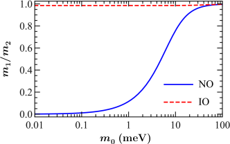
Figure 1: The mass ratio $m_{1}/m_{2}$ for NO and IO.

The Fig. 1 shows the ratio of $m_{1}/m_{2}$ as a function of the lightest mass, $m_{0}\equiv m_{1}$ for NO and $m_{0}\equiv m_{3}$ for IO. Since the atmospheric mass splitting is much larger than the solar one, $\Delta m^{2}_{s}/\Delta m^{2}_{a}\approx 3\%\ll 1$, $m_{1}$ and $m_{2}$ are almost degenerate across the whole parameter space for IO. In contrast, they can be non-degenerate for NO. With $m_{1}\lesssim 40\,\mbox{meV}$, there is apparent deviation from being degenerate. The smaller $m_{1}$, the bigger the deviation.

As expected, there is no visible difference between the solar octants for IO while for NO the effect is sizeable, as shown in Fig. 2. For IO, the predictions with LO and HO almost completely overlap with each other. So we show only one case in green color and label it as “IO”. For NO, the prediction with LO (in red color and labeled as “NO-LO”) is totally different from the one with HO (in blue color and labeled as “NO-HO”). Especially, the funnel region for NO-LO completely disappears for NO-HO. Instead, the effective mass $|m_{ee}|$ is bounded from below across the whole parameter range. The different effective mass distributions between NO-LO and NO-HO as well as the degenerate distributions between IO-LO and IO-HO N.:2019cot is actually a reflection of the $m_{1}$–$m_{2}$ non-degeneracy or degeneracy, respectively.

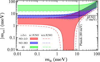
Figure 2: The allowed range of $|m_{ee}|$ for NO with LO (NO-LO, red), NO with HO (NO-HO, blue), and IO (green). The dashed lines indicate the $3\sigma$ uncertainty according to the current global fit deSalas:2018bym ; Esteban:2018azc of neutrino oscillation parameters ($\theta_{s}$, $\theta_{r}$, $\Delta m^{2}_{s}$, and $\Delta m^{2}_{a}$) while for the filled region we further impose the projected precision of $\sin^{2}\theta_{s}$ (0.54%) and $\Delta m_{s}^{2}$ (0.24%) at the future JUNO experiment An:2015jdp . For comparison, the typical future prospects of the $0\nu 2\beta$ decay measurement Kharusi:2018eqi and cosmological constraint Dvorkin:2019jgs ; RoyChoudhury:2019hls are shown as horizontal and vertical lines, respectively.

According to the geometrical picture Xing:2014yka , the lower and upper limits are completely determined by the lengths of the three complex vectors, ($L^{\rm LO}_{1}\equiv c^{2}_{r}c^{2}_{s}m_{1}$, $L^{\rm LO}_{2}\equiv c^{2}_{r}s^{2}_{s}m_{2}$, and $L_{3}\equiv s^{2}_{r}m_{3}$ for LO). With $m_{1}$ and $m_{2}$ switched, namely $L^{\rm HO}_{1}\equiv c^{2}_{r}s^{2}_{s}m_{1}$ and $L^{\rm HO}_{2}\equiv c^{2}_{r}c^{2}_{s}m_{2}$ for HO, the situation becomes totally different from the LO case. For convenience, we use only the LO value for the solar angle, $\theta_{s}<\pi/4$, globally. As shown in Fig. 3, $L^{\rm HO}_{2}>L^{\rm HO}_{1}+L_{3}$ holds for the whole parameter space. Consequently, the lower limit of the effective mass is always $|m_{ee}|^{\rm NO-HO}_{min}=L^{\rm HO}_{2}-L^{\rm HO}_{1}-L_{3}$. Most importantly, $L^{\rm HO}_{2}$ never crosses with $L^{\rm HO}_{1}+L_{3}$ since interchanging $c_{s}\approx\sqrt{2/3}$ and $s_{s}\approx\sqrt{1/3}$ to switch from LO to HO can significantly amplify $L^{\rm HO}_{2}$ and suppress $L^{\rm HO}_{1}$. This is especially true for small $m_{1}$ and hence small $m_{1}/m_{2}$. Although $L_{3}$ contains the largest mass eigenvalue $m_{3}$, the suppression of $s^{2}_{r}$ makes $L_{3}$ too small to compensate the difference between $L^{\rm HO}_{1}$ and $L^{\rm HO}_{2}$, and hence the inequality $L^{\rm HO}_{2}>L^{\rm HO}_{1}+L_{3}$ always holds. For comparison, the boundary parameters for NO-LO can be found in Fig. 10b of Ge:2016tfx .

Although the lower boundary for the effective mass $|m_{ee}|$ with NO-HO is established, the prediction can still receive significant uncertainty from the neutrino oscillation parameters for both the lower and upper boundaries, shown as the regions between the dashed curves for the $3\sigma$ variations in Fig. 2. As argued in similar situations Ge:2016tfx ; Dueck:2011hu ; Ge:2015bfa , the largest variation comes from the uncertainties in the solar angle $\theta_{s}$. This is the place where the intermediate baseline reactor neutrino experiment JUNO An:2015jdp can help. The precision measurement on the solar angle $\theta_{s}$ comes from the slow oscillation modulated by the smaller solar mass splitting $\Delta m^{2}_{s}$ Ge:2012wj ; Ge:2015bfa ,

$$P_{ee}=1-\cos^{4}\theta_{r}\sin^{2}2\theta_{s}\sin^{2}\Delta_{s}+\cdots\,,$$ (3)

where $\Delta_{s}\equiv\Delta m^{2}_{s}L/4E_{\nu}$ while $\cdots$ stands for the higher

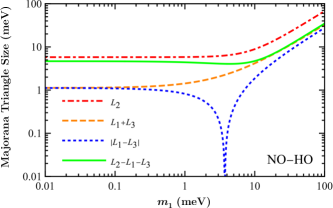
Figure 3: The relevant boundary parameters for NO-HO.

frequency modes modulated by the larger atmospheric mass splitting $\Delta m^{2}_{a}$ and its variation $\Delta m^{2}_{a}-\Delta m^{2}_{s}$. The above Eq. (3) clearly indicates that the constraint on the solar angle is in the form of $\sin^{2}2\theta_{s}=4c^{2}_{s}s^{2}_{s}$, instead of the individual $c_{s}$ or $s_{s}$. The simulations found that $\sin^{2}\theta_{s}$ can be measured with $0.54\%$ precision Ge:2012wj ; An:2015jdp ; Li:2016txk , from which the uncertainty of the individual $s^{2}_{s}$ can be extracted as

$$\delta s^{2}_{s}=2c_{s}s_{s}\delta\theta_{s}=\frac{c^{2}_{s}s^{2}_{s}}{c^{2}_{s}-s^{2}_{s}}\frac{\delta\sin^{2}2\theta_{s}}{\sin^{2}2\theta_{s}}\,.$$ (4)

The right-hand side of Eq. (4) is invariant under the octant transformation $c_{s}\leftrightarrow s_{s}$, regardless of an overall minus sign. Since the coefficient $2c_{s}s_{s}$ of the solar angle variation $\delta\theta_{s}$ is also invariant under the octant transformation, the absolute uncertainty of the solar angle is not affected, no matter which octant it rests in. The JUNO experiment precision on the solar angle is quite robust against the solar octant degeneracy and we can directly use the simulated precision from the JUNO Yellow Book An:2015jdp .

The filled regions in Fig. 2 show the $3\sigma$ range after taking JUNO into account. Adding JUNO significantly reduces the uncertainty in the predicted effective mass, which already seems significant in a log scale plot. Especially, in the vanishing mass limit, $m_{1}\rightarrow 0$, the two regions of NO-LO and NO-HO overlap with each other when taking the current global fit values of the oscillation parameters and separate from each other after combining the projected JUNO result. For $m_{1}<0.4~{}{\rm meV}$, the NO-HO and NO-LO distributions detach from each other. Since the lightest mass eigenvalue $m_{1}$ is negligible in this range, the upper limit for NO-LO, $|m_{ee}|^{\rm NO-LO}_{\rm max}=L^{\rm LO}_{2}+L_{3}$, and the lower limit for NO-HO, $|m_{ee}|^{\rm NO-HO}_{\rm min}=L^{\rm HO}_{2}-L_{3}$ are fully determined by the $m_{2}$ and $m_{3}$ terms. The difference between these two limits is, $L^{\rm HO}_{2}-L^{\rm LO}_{2}-2L_{3}=c^{2}_{r}(c^{2}_{s}-s^{2}_{s})m_{2}-2s^{2}_{r}m_{3}$. Since the ratio of the coefficients $2s^{2}_{r}/[c^{2}_{r}(c^{2}_{s}-s^{2}_{s})]\approx 6s^{2}_{r}\approx 13.4\%$ is smaller than $m_{2}/m_{3}\approx\sqrt{\Delta m^{2}_{s}/\Delta m^{2}_{a}}\approx 17.1\%$, $|m_{ee}|^{\rm NO-HO}_{\rm min}-|m_{ee}|^{\rm NO-LO}_{\rm max}$ is always positive. To avoid overlap between the NO-LO and NO-HO regions, the solar angle cannot be too large,

$$\cos 2\theta_{s}\gtrsim\frac{2s^{2}_{r}\sqrt{\Delta m^{2}_{a}}}{c^{2}_{r}\sqrt{\Delta m^{2}_{s}}}\approx 26.8\%\quad\Rightarrow\quad\theta_{s}\lesssim 37.2^{\circ}\,,$$ (5)

where the boundary is more than $4\sigma$ away from the current experimental best-fit value deSalas:2018bym ; Esteban:2018azc . In other words, even considering the fact that the best-fit value of $\sin^{2}2\theta_{s}$ could vary, it is highly unlikely that the NO-LO and NO-HO regions can overlap in the range of $m_{1}\lesssim 0.4~{}{\rm meV}$. Having $s^{2}_{s}\approx 1/3$ so that the missing solar neutrino measurements consistently measured $1/3$ of the predicted flux is not just a coincidence. The solar angle not being too large so that the $0\nu 2\beta$ decay can optimize the chance for excluding the solar HO solution adds one more argument to the advertised intelligent design of neutrino parameters Goodman ; Wojcicki .

Since the JUNO experiment can measure $(\sin^{2}\theta_{s},\Delta m_{s}^{2},\Delta m_{a}^{2})$ with better than $1\%$ precision An:2015jdp and the Daya Bay experiment can measure $\sin^{2}2{\theta}_{r}$ with $3\%$ precision Cao:2017drk , the remaining uncertainty mainly comes from the $0\nu 2\beta$ decay measurement itself, including the effective mass sensitivity $\sigma_{|m_{ee}|^{2}}$ and its central value $|m_{ee}|^{2}_{\rm c}$, as well as the uncertainty of the cosmological constraint on the neutrino mass sum, $\sigma_{\rm sum}$. For both observations, we assume Gaussian distribution with central value at zero unless stated otherwise. The direct observable in $0\nu 2\beta$ experiments is the event rate that follows the exponential law, $N(t)=N_{0}e^{-t/T}$, where $T$ is the corresponding lifetime. From the measured signal event number $\Delta N=N_{0}\Delta t/T$ within the experimental exposure time $\Delta t\ll T$, the decay lifetime can be derived, $T=N_{0}\Delta t/\Delta N$. Conventionally, the lifetime can be equivalently denoted as the half-lifetime, $T_{1/2}\equiv T\ln 2=1/(G|M|^{2}|m_{ee}|^{2})$, where $G$ is the phase space factor and $M$ denotes the nuclear matrix element. The lifetime $T$ is measured experimentally while the phase factor $G$ and the nuclear matrix element come from theoretical calculations. The effective mass is then obtained as, $|m_{ee}|^{2}=1/(G|M|^{2}T\ln 2)$. The major uncertainty comes from the experimental one in the lifetime measurement and the theoretical one in the nuclear matrix element calculation, both contributing to the uncertainty $\sigma_{|m_{ee}|^{2}}$,

$$P_{0\nu 2\beta}(|m_{ee}|^{2})=\frac{1}{\sqrt{2\pi}\sigma_{|m_{ee}|^{2}}}e^{-\frac{\left(|m_{ee}|^{2}-|m_{ee}|^{2}_{\rm c}\right)^{2}}{2\sigma_{|m_{ee}|^{2}}^{2}}}$$ (6)

For generality, we introduce the central value $|m_{ee}|^{2}_{\rm c}$. If no event is observed, the distribution peaks at vanishing $\Delta N$ or $|m_{ee}|_{\rm c}=0$. Similarly, we assume the Gaussian probability distribution of the sum of neutrino masses to be:

$$P_{\rm cosmo}\left(\sum_{i}m_{i}\right)=\frac{1}{\sqrt{2\pi}\sigma_{\rm sum}}e^{-\frac{\left(\sum_{i}m_{i}\right)^{2}}{2\sigma_{\rm sum}^{2}}}\;.$$ (7)

As pointed out above, the combined JUNO An:2015jdp measurement and Daya Bay Adey:2018zwh ; Cao:2017drk can significantly reduce the uncertainties from the oscillation parameters to make them negligibly small compared with the uncertainties from the $0\nu 2\beta$ decay measurement itself. So we fix the oscillation parameters ($\theta_{r}$, $\theta_{s}$, $\Delta m^{2}_{a}$, and $\Delta m^{2}_{s}$) to their current best fit values deSalas:2018bym ; Esteban:2018azc in the following discussions. The only remaining parameters are just the two Majorana CP phases ($\tilde{\delta}_{\rm M1}$ and $\tilde{\delta}_{\rm M3}$) and the lightest mass $m_{0}$. Given a particular mass ordering (NO or IO), its corresponding likelihood $\mathcal{L}_{\rm MO}(\sigma_{|m_{ee}|^{2}},\sigma_{\rm sum})$ can be evaluated as

$$\int P_{0\nu 2\beta}\left(|m_{ee}|^{2}_{\rm MO}\right)P_{\rm cosmo}\left(\sum_{i}m_{i}\right){\rm d}m_{0}\frac{{\rm d}\tilde{\delta}_{\rm M1}}{2\pi}\frac{{\rm d}\tilde{\delta}_{\rm M3}}{2\pi}\,,\quad$$ (8)

where $m_{0}=m_{1}(m_{3})$ for MO = NO (IO), respectively. The relative probability

$$P_{\rm NO,IO}\equiv\frac{\mathcal{L}_{\rm NO,IO}}{\mathcal{L}_{\rm NO}+\mathcal{L}_{\rm IO}}$$ (9)

quantifies how well the normal (inverted) mass ordering fits the observations, namely, the NO (IO) sensitivity. We show how $P_{\rm NO}$ changes with different $\sigma_{\rm sum}$ and $\sigma_{|m_{ee}|^{2}}$ in Fig. 4, assuming no $0\nu 2\beta$ decay is observed and hence $|m_{ee}|_{c}=0$. For $\sqrt{\sigma_{|m_{ee}|^{2}}}\gtrsim 50\,\mbox{meV}$, the NO sensitivity mainly comes from the cosmological constraint and otherwise from the $0\nu 2\beta$ decay. Around $\sqrt{\sigma_{|m_{ee}|^{2}}}\sim 50\,\mbox{meV}$, the two mass orderings can already be distinguished with sensitivity $P_{\rm NO}\approx 0.7$. In other words, the NO can be identified with ${\cal O}(10\,{\rm meV})$ sensitivity of $\sqrt{\sigma_{|m_{ee}|^{2}}}$.

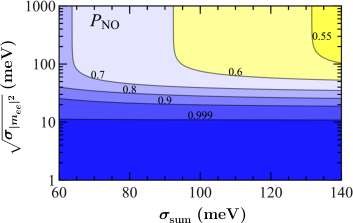
Figure 4: The relative probability of NO as a function of the cosmological sensitivity ($\sigma_{\rm sum}$) and the $0\nu 2\beta$ decay sensitivity ($\sigma_{|m_{ee}|^{2}}$).

After establishing the NO, distinguishing the solar octants takes the similar definition,

$$P_{\rm LO,HO}\equiv\frac{{\cal L}_{\rm NO-LO,HO}}{{\cal L}_{\rm NO-LO}+{\cal L}_{\rm NO-HO}}\,,$$ (10)

to quantify the probability that the lower (higher) solar octant is favored. Fig. 5 illustrates the values of $P_{\rm LO}$ with different $\sqrt{\sigma_{|m_{ee}|^{2}}}$ and $|m_{ee}|_{\rm c}$. It is possible to exclude the NO-HO solution if the $0\nu 2\beta$ decay sensitivity further improves to $\sqrt{\sigma_{|m_{ee}|^{2}}}\lesssim 4\,\mbox{meV}$. According to Fig. 2, the lowest point of the lower boundary for NO-HO is $|m_{ee}|=3.2\,\mbox{meV}$ at $m_{1}=5.3\,\mbox{meV}$ without JUNO or $|m_{ee}|=3.8\,\mbox{meV}$ at $m_{1}=4.5\,\mbox{meV}$ with JUNO, lower than $4\,\mbox{meV}$ N.:2019cot ; Deepthi:2019ljo . However, the realistic measurement has no clear cut. As long as the $0\nu 2\beta$ sensitivity $\sqrt{\sigma_{|m_{ee}|^{2}}}$ goes below $10\,\mbox{meV}$, which is within the exploration range of future experiments such as nEXO Kharusi:2018eqi and the proposed JUNO-LS detector Zhao:2016brs , the possibility for excluding the NO-HO solution can appear: If the $0\nu 2\beta$ decay is not observed, the NO-HO solution can be excluded, with external input of the Majorana nature of neutrinos nu-collider ; nc-scattering ; nu-antinu1 ; nu-antinu2 ; nu-antinu3 ; nu-antinu4 ; nu-antinu5 ; nu-antinu6 ; nu-antinu7 ; Majorana-EMD1 ; Majorana-EMD2 ; Majorana-EMD3 ; CNB . Note that there are already quite a few discussions on the prospect of the $\mathcal{O}(\mbox{meV})$ sensitivity of $|m_{ee}|$ Kharusi:2018eqi ; Agostini:2017jim ; Xing:2015zha ; Ge:2016tfx ; Cao:2019hli ; Penedo:2018kpc ; Revealing from both experimental and theoretical perspectives.

The Two Majorana CP Phases – If the $0\nu 2\beta$ decay sensitivity further improves to the sub-meV scale, it is then possible to simultaneously determine the two Majorana CP phases Xing:2015zha ; Ge:2016tfx ; Cao:2019hli . The basic logic is that the three complex vectors in Eq. (2) form a closed Majorana triangle on the complex plane if the effective mass $|m_{ee}|$ vanishes. Once the lengths $L_{i}$ of its three sides are known, its three inner angles can be uniquely determined as functions of $L_{i}$. Two of the three inner angles are actually the two Majorana CP phases as defined in Eq. (2).

Observing the $0\nu 2\beta$ decay indicates a nonzero effective mass $|m_{ee}|$, corresponding to only one degree of freedom. Then only one combination of the two Majorana CP phases can be determined or constrained. But a vanishing effective mass, $|m_{ee}|=0$, yields two independent constraints, $m_{ee}=0$ or more explicitly, $\mathbb{R}(m_{ee})=\mathbb{I}(m_{ee})=0$, where $\mathbb{R}$ and $\mathbb{I}$ extract the real and imaginary components, respectively. Two constraints can resolve two degrees of freedom, explaining why the two Majorana CP phases can be simultaneously determined. The same situation can happen for the more realistic case with some upper limit $U$, $|m_{ee}|\leq U$, which can convert to two independent upper limits, $\mathbb{R}(m_{ee})\leq U$ and $\mathbb{I}(m_{ee})\leq U$. The two Majorana CP phases are then determined/constrained within some contour. Again, the JUNO An:2015jdp and Daya Bay Cao:2017drk experiments can play an important role by significantly reducing the experimental uncertainties from the oscillation parameters.

This simultaneous determination of the two Majorana CP phases can only happen when the effective mass $|m_{ee}|$ falls into the funnel region and hence only for NO. With IO, one physical degree of freedom would become invisible forever, which is a big loss for physics search. In contrast, NO makes it possible to measure all physical variables without losing any information. No physical degrees of freedom would be missing.

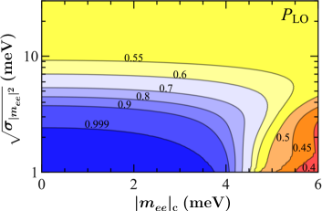
Figure 5: The relative probability of NO-LO from the $0\nu 2\beta$ decay effective mass sensitivity ($\sigma_{|m_{ee}|^{2}}$) and its central value ($|m_{ee}|^{2}_{\rm c}$).

It seems that the vanishing $|m_{ee}|$ is a disappointing future for the $0\nu 2\beta$ decay experiments, which is not necessarily true. The prospect of simultaneously determining the two Majorana CP phases provides a continuous motivation for improving the experimental sensitivity. Either we can verify the Majorana nature or measure the two Majorana CP phases. Both are physically important. To some extent, the $0\nu 2\beta$ decay has no-loss future. With other alternative measurements providing the Majorana nature nu-collider ; nc-scattering ; nu-antinu1 ; nu-antinu2 ; nu-antinu3 ; nu-antinu4 ; nu-antinu5 ; nu-antinu6 ; nu-antinu7 ; Majorana-EMD1 ; Majorana-EMD2 ; Majorana-EMD3 ; CNB , the $0\nu 2\beta$ experiment can simultaneously measure the two Majorana CP phases.

Conclusion – We envision the future prospect of neutrino mass ordering and its role in the $0\nu 2\beta$ decay by assuming the Majorana nature of neutrinos. The NO is not the seemingly boring option or “God’s Mistake”, but can lead to much more vivid landscapes. First, with $\mathcal{O}(10\,\mbox{meV})$ sensitivity on the effective mass $|m_{ee}|$, the $0\nu 2\beta$ decay measurement can distinguish NO from IO. Second, if the sensitivity further improves to $\mathcal{O}(\mbox{meV})$, the $0\nu 2\beta$ decay measurement can exclude the solar HO. Different from the NO-LO option that has a funnel region in the effective mass distribution, the effective mass of the NO-HO option is bounded from below, $|m_{ee}|\geq 3.2\,(3.8)\,\mbox{meV}$ without (with) input from JUNO. The solar angle is at the right value to separate the NO-LO region from the NO-HO one with vanishing or relatively small $m_{1}$. Finally, if the sensitivity improves even further to sub-meV, NO allows the two Majorana CP phases to be simultaneously determined in the absence of the $0\nu 2\beta$ decay signal, observing all physical degrees of freedom. During this adventure, the input of the solar angle from JUNO and the Majorana nature from independent measurements are necessary. The rich mine in the $0\nu 2\beta$ decay is just starting to appear and the global fit preference of NO is not a nightmare, but an inspiring herald of a new era.

References

- (1) B. Pontecorvo, “Mesonium and anti-mesonium,” Sov. Phys. JETP 6, 429 (1957) [Zh. Eksp. Teor. Fiz. 33, 549 (1957)].
- (2) Z. Maki, M. Nakagawa and S. Sakata, “Remarks on the unified model of elementary particles,” Prog. Theor. Phys. 28, 870 (1962).
- (3) M. Tanabashi et al. [Particle Data Group], “Review of Particle Physics,” Phys. Rev. D 98, no. 3, 030001 (2018).
- (4) S. F. Ge and S. J. Parke, “Scalar Nonstandard Interactions in Neutrino Oscillation,” Phys. Rev. Lett. 122, no. 21, 211801 (2019) [arXiv:1812.08376 [hep-ph]].
- (5) S. F. Ge and H. Murayama, “Apparent CPT Violation in Neutrino Oscillation from Dark Non-Standard Interactions,” [arXiv:1904.02518 [hep-ph]].
- (6) S. F. Ge, “Neutrino Matter Effect & (vector, scalar, dark) Non-Standard Interactions”, Workshop of Jinping Neutrino Experiment 2019, Beijing, China, July 27, 2019.
- (7) S. F. Ge, “Leptonic CP Measurement & New Physics”, The 21st International Workshop on Neutrinos from Accelerators (NUFACT2019), Daegu, Korea, August 29, 2019.
- (8) S. F. Ge, “New Physics & (vector, scalar, dark) NSI’s”, The 16th International Conference on Topics in Astroparticle and Underground Physics (TAUP 2019), Toyama, Japan, September 10, 2019.
- (9) K. Y. Choi, E. J. Chun and J. Kim, “Neutrino Oscillations in Dark Matter,” Phys. Dark Univ. 30, 100606 (2020) [arXiv:1909.10478 [hep-ph]].
- (10) P. F. De Salas, S. Gariazzo, O. Mena, C. A. Ternes and M. Tórtola, “Neutrino Mass Ordering from Oscillations and Beyond: 2018 Status and Future Prospects,” Front. Astron. Space Sci. 5, 36 (2018) [arXiv:1806.11051 [hep-ph]];
- (11) I. Esteban, M. C. Gonzalez-Garcia, A. Hernandez-Cabezudo, M. Maltoni and T. Schwetz, “Global analysis of three-flavour neutrino oscillations: synergies and tensions in the determination of , and the mass ordering,” JHEP 1901, 106 (2019) [arXiv:1811.05487 [hep-ph]]; NuFIT 4.1 (2019), www.nu-fit.org.
- (12) S. Wojcicki, Private communication with Maury Goodman.
- (13) Maury Goodman, “Neutrino mistakes: wrong tracks and hints, hopes and failures”, History of the Neutrino, September 5-7, 2018, Paris, France [arXiv:1901.07068 [hep-ex]].
- (14) L. Wolfenstein, “Neutrino Oscillations in Matter,” Phys. Rev. D 17, 2369 (1978).
- (15) S. P. Mikheyev and A. Y. Smirnov, “Resonance Amplification of Oscillations in Matter and Spectroscopy of Solar Neutrinos,” Sov. J. Nucl. Phys. 42, 913 (1985) [Yad. Fiz. 42, 1441 (1985)].
- (16) S. P. Mikheev and A. Y. Smirnov, “Resonant amplification of neutrino oscillations in matter and solar neutrino spectroscopy,” Nuovo Cim. C 9, 17 (1986).
- (17) S. P. Mikheev and A. Y. Smirnov, “Neutrino Oscillations in a Variable Density Medium and Neutrino Bursts Due to the Gravitational Collapse of Stars,” Sov. Phys. JETP 64, 4 (1986) [Zh. Eksp. Teor. Fiz. 91, 7 (1986)] [arXiv:0706.0454 [hep-ph]].
- (18) S. Roy Choudhury and S. Hannestad, “Updated results on neutrino mass and mass hierarchy from cosmology with Planck 2018 likelihoods,” JCAP 07, 037 (2020) [arXiv:1907.12598 [astro-ph.CO]].
- (19) S. F. Ge and M. Lindner, “Extracting Majorana properties from strong bounds on neutrinoless double beta decay,” Phys. Rev. D 95, no. 3, 033003 (2017) [arXiv:1608.01618 [hep-ph]].
- (20) Z. z. Xing, “Flavor structures of charged fermions and massive neutrinos,” Phys. Rept. 854, 1-147 (2020) [arXiv:1909.09610 [hep-ph]].
- (21) S. Weinberg, “Baryon and Lepton Nonconserving Processes,” Phys. Rev. Lett. 43, 1566 (1979).
- (22) T.Yanagida, “Neutrino Mass and Horizontal Symmetry”, Proceedings of INS International Symposium on Quark and Lepton Physics, edited by K. Fujikawa, H. Terazawa, and A. Ukawa (University of Tokyo, Tokyo,1981), C81-06-25, pp. 233-237.
- (23) H. Fritzsch, M. Gell-Mann and P. Minkowski, “Vector - Like Weak Currents and New Elementary Fermions,” Phys. Lett. B 59, 256 (1975).
- (24) P. Minkowski, “ at a Rate of One Out of Muon Decays?,” Phys. Lett. B 67, 421 (1977).
- (25) T. Yanagida, “Horizontal gauge symmetry and masses of neutrinos,” Conf. Proc. C 7902131, 95 (1979).
- (26) M. Gell-Mann, P. Ramond and R. Slansky, “Complex Spinors and Unified Theories,” Conf. Proc. C 790927, 315 (1979) [arXiv:1306.4669 [hep-th]].
- (27) S. L. Glashow, “The Future of Elementary Particle Physics,” NATO Sci. Ser. B 61, 687 (1980).
- (28) R. N. Mohapatra and G. Senjanovic, “Neutrino Mass and Spontaneous Parity Nonconservation,” Phys. Rev. Lett. 44 (1980) 912.
- (29) W. Konetschny and W. Kummer, “Nonconservation of Total Lepton Number with Scalar Bosons,” Phys. Lett. 70B, 433 (1977).
- (30) T. P. Cheng and L. F. Li, “Neutrino Masses, Mixings and Oscillations in SU(2) x U(1) Models of Electroweak Interactions,” Phys. Rev. D 22, 2860 (1980).
- (31) J. Schechter and J. W. F. Valle, “Neutrino Masses in SU(2) x U(1) Theories,” Phys. Rev. D 22, 2227 (1980).
- (32) G. B. Gelmini and M. Roncadelli, “Left-Handed Neutrino Mass Scale and Spontaneously Broken Lepton Number,” Phys. Lett. 99B, 411 (1981).
- (33) R. Foot, H. Lew, X. G. He and G. C. Joshi, “Seesaw Neutrino Masses Induced by a Triplet of Leptons,” Z. Phys. C 44, 441 (1989).
- (34) M. Fukugita and T. Yanagida, “Baryogenesis Without Grand Unification,” Phys. Lett. B 174, 45 (1986).
- (35) K. S. Babu and R. N. Mohapatra, “Is There a Connection Between Quantization of Electric Charge and a Majorana Neutrino?,” Phys. Rev. Lett. 63, 938 (1989).
- (36) K. S. Babu and R. N. Mohapatra, “Quantization of Electric Charge From Anomaly Constraints and a Majorana Neutrino,” Phys. Rev. D 41, 271 (1990).
- (37) P. Coloma and T. Schwetz, “Generalized mass ordering degeneracy in neutrino oscillation experiments,” Phys. Rev. D 94, no. 5, 055005 (2016) Erratum: [Phys. Rev. D 95, no. 7, 079903 (2017)] [arXiv:1604.05772 [hep-ph]].
- (38) E. K. Akhmedov, P. Huber, M. Lindner and T. Ohlsson, “T violation in neutrino oscillations in matter,” Nucl. Phys. B 608, 394 (2001) [arXiv:hep-ph/0105029].
- (39) P. Coloma, M. C. Gonzalez-Garcia, M. Maltoni and T. Schwetz, “COHERENT Enlightenment of the Neutrino Dark Side,” Phys. Rev. D 96, no. 11, 115007 (2017) [arXiv:1708.02899 [hep-ph]].
- (40) C. Giunti, “General COHERENT Constraints on Neutrino Non-Standard Interactions,” Phys. Rev. D 101, no.3, 035039 (2020) [arXiv:1909.00466 [hep-ph]].
- (41) O. G. Miranda, M. A. Tortola and J. W. F. Valle, “Are solar neutrino oscillations robust?,” JHEP 0610, 008 (2006) [hep-ph/0406280].
- (42) F. J. Escrihuela, O. G. Miranda, M. A. Tortola and J. W. F. Valle, “Constraining nonstandard neutrino-quark interactions with solar, reactor and accelerator data,” Phys. Rev. D 80, 105009 (2009) Erratum: [Phys. Rev. D 80, 129908 (2009)] [arXiv:0907.2630 [hep-ph]].
- (43) Y. Farzan, “A model for large non-standard interactions of neutrinos leading to the LMA-Dark solution,” Phys. Lett. B 748, 311 (2015) [arXiv:1505.06906 [hep-ph]].
- (44) Y. Farzan and I. M. Shoemaker, “Lepton Flavor Violating Non-Standard Interactions via Light Mediators,” JHEP 1607, 033 (2016) [arXiv:1512.09147 [hep-ph]].
- (45) D. V. Forero and W. C. Huang, “Sizable NSI from the SU(2)L scalar doublet-singlet mixing and the implications in DUNE,” JHEP 1703, 018 (2017) [arXiv:1608.04719 [hep-ph]].
- (46) K. S. Babu, A. Friedland, P. A. N. Machado and I. Mocioiu, “Flavor Gauge Models Below the Fermi Scale,” JHEP 1712, 096 (2017) [arXiv:1705.01822 [hep-ph]].
- (47) Y. Farzan and M. Tortola, “Neutrino oscillations and Non-Standard Interactions,” Front. in Phys. 6, 10 (2018) [arXiv:1710.09360 [hep-ph]].
- (48) P. B. Denton, Y. Farzan and I. M. Shoemaker, “Testing large non-standard neutrino interactions with arbitrary mediator mass after COHERENT data,” JHEP 1807, 037 (2018) [arXiv:1804.03660 [hep-ph]].
- (49) P. Coloma, P. B. Denton, M. C. Gonzalez-Garcia, M. Maltoni and T. Schwetz, “Curtailing the Dark Side in Non-Standard Neutrino Interactions,” JHEP 1704, 116 (2017) [arXiv:1701.04828 [hep-ph]].
- (50) I. Esteban, M. C. Gonzalez-Garcia, M. Maltoni, I. Martinez-Soler and J. Salvado, “Updated Constraints on Non-Standard Interactions from Global Analysis of Oscillation Data,” JHEP 1808, 180 (2018) [arXiv:1805.04530 [hep-ph]].
- (51) P. Coloma, I. Esteban, M. C. Gonzalez-Garcia and M. Maltoni, “Improved global fit to Non-Standard neutrino Interactions using COHERENT energy and timing data,” JHEP 02, 023 (2020) [arXiv:1911.09109 [hep-ph]].
- (52) Y. F. Li, Y. Wang and Z. z. Xing, “Terrestrial matter effects on reactor antineutrino oscillations at JUNO or RENO-50: how small is small?,” Chin. Phys. C 40, no. 9, 091001 (2016) [arXiv:1605.00900 [hep-ph]].
- (53) K. N. Vishnudath, S. Choubey and S. Goswami, “New sensitivity goal for neutrinoless double beta decay experiments,” Phys. Rev. D 99, no. 9, 095038 (2019) [arXiv:1901.04313 [hep-ph]].
- (54) Y. Farzan and A. Y. Smirnov, “On the effective mass of the electron neutrino in beta decay,” Phys. Lett. B 557, 224 (2003) [hep-ph/0211341].
- (55) S. A. Kharusi et al. [nEXO Collaboration], “nEXO Pre-Conceptual Design Report,” [arXiv:1805.11142 [physics.ins-det]].
- (56) C. Dvorkin et al., “Neutrino Mass from Cosmology: Probing Physics Beyond the Standard Model,” [arXiv:1903.03689 [astro-ph.CO]].
- (57) Z. z. Xing and Y. L. Zhou, “Geometry of the effective Majorana neutrino mass in the decay,” Chin. Phys. C 39, 011001 (2015) [arXiv:1404.7001 [hep-ph]].
- (58) A. Dueck, W. Rodejohann and K. Zuber, “Neutrinoless Double Beta Decay, the Inverted Hierarchy and Precision Determination of theta(12),” Phys. Rev. D 83, 113010 (2011) [arXiv:1103.4152 [hep-ph]].
- (59) S. F. Ge and W. Rodejohann, “JUNO and Neutrinoless Double Beta Decay,” Phys. Rev. D 92, no. 9, 093006 (2015) [arXiv:1507.05514 [hep-ph]].
- (60) F. An et al. [JUNO Collaboration], “Neutrino Physics with JUNO,” J. Phys. G 43, no. 3, 030401 (2016) [arXiv:1507.05613 [physics.ins-det]].
- (61) S. F. Ge, K. Hagiwara, N. Okamura and Y. Takaesu, “Determination of mass hierarchy with medium baseline reactor neutrino experiments,” JHEP 1305, 131 (2013) [arXiv:1210.8141 [hep-ph]].
- (62) L. J. W. J. Cao and Y. F. Wang, “Reactor Neutrino Experiments: Present and Future,” Ann. Rev. Nucl. Part. Sci. 67, 183 (2017) [arXiv:1803.10162 [hep-ex]].
- (63) D. Adey et al. [Daya Bay Collaboration], “Measurement of the Electron Antineutrino Oscillation with 1958 Days of Operation at Daya Bay,” Phys. Rev. Lett. 121, 241805 (2018) [arXiv:1809.02261 [hep-ex]].
- (64) K. N. Deepthi, S. Goswami, V. K. N. and T. K. Poddar, “Implications of the Dark LMA solution and Fourth Sterile Neutrino for Neutrino-less Double Beta Decay,” [arXiv:1909.09434 [hep-ph]].
- (65) J. Zhao, L. J. Wen, Y. F. Wang and J. Cao, “Physics potential of searching for decays in JUNO,” Chin. Phys. C 41, 053001 (2017) [arXiv:1610.07143 [hep-ex]].
- (66) W. Rodejohann, “Inverse Neutrino-less Double Beta Decay Revisited: Neutrinos, Higgs Triplets and a Muon Collider,” Phys. Rev. D 81, 114001 (2010) [arXiv:1005.2854 [hep-ph]].
- (67) B. Kayser and R. E. Shrock, “Distinguishing Between Dirac and Majorana Neutrinos in Neutral Current Reactions,” Phys. Lett. B 112, 137-142 (1982).
- (68) J. Schechter and J. W. F. Valle, “Neutrino Oscillation Thought Experiment,” Phys. Rev. D 23, 1666 (1981).
- (69) L. F. Li and F. Wilczek, “Physical Processes Involving Majorana Neutrinos,” Phys. Rev. D 25, 143 (1982).
- (70) J. Bernabeu and P. Pascual, “CP Properties of the Leptonic Sector for Majorana Neutrinos,” Nucl. Phys. B 228, 21 (1983).
- (71) P. Langacker and J. Wang, “Neutrino anti-neutrino transitions,” Phys. Rev. D 58, 093004 (1998) [arXiv:hep-ph/9802383].
- (72) A. de Gouvea, B. Kayser and R. N. Mohapatra, “Manifest CP violation from Majorana phases,” Phys. Rev. D 67, 053004 (2003) [arXiv:hep-ph/0211394].
- (73) Z. z. Xing, “Properties of CP Violation in Neutrino-Antineutrino Oscillations,” Phys. Rev. D 87, no. 5, 053019 (2013) [arXiv:1301.7654 [hep-ph]].
- (74) Z. z. Xing and Y. L. Zhou, “Majorana CP-violating phases in neutrino-antineutrino oscillations and other lepton-number-violating processes,” Phys. Rev. D 88, 033002 (2013) [arXiv:1305.5718 [hep-ph]].
- (75) B. Kayser, “Majorana Neutrinos and their Electromagnetic Properties,” Phys. Rev. D 26, 1662 (1982).
- (76) N. F. Bell, V. Cirigliano, M. J. Ramsey-Musolf, P. Vogel and M. B. Wise, “How magnetic is the Dirac neutrino?,” Phys. Rev. Lett. 95, 151802 (2005) [hep-ph/0504134].
- (77) N. F. Bell, M. Gorchtein, M. J. Ramsey-Musolf, P. Vogel and P. Wang, “Model independent bounds on magnetic moments of Majorana neutrinos,” Phys. Lett. B 642, 377 (2006) [hep-ph/0606248].
- (78) Cosmic neutrino background: A. J. Long, C. Lunardini and E. Sabancilar, “Detecting non-relativistic cosmic neutrinos by capture on tritium: phenomenology and physics potential,” JCAP 1408, 038 (2014) [arXiv:1405.7654 [hep-ph]].
- (79) M. Agostini, G. Benato and J. Detwiler, “Discovery probability of next-generation neutrinoless double- decay experiments,” Phys. Rev. D 96, 053001 (2017) [arXiv:1705.02996 [hep-ex]].
- (80) Z. z. Xing, Z. h. Zhao and Y. L. Zhou, “How to interpret a discovery or null result of the decay,” Eur. Phys. J. C 75, no. 9, 423 (2015) [arXiv:1504.05820 [hep-ph]].
- (81) J. Cao, G. Y. Huang, Y. F. Li, Y. Wang, L. J. Wen, Z. z. Xing, Z. H. Zhao and S. Zhou, “Towards the meV limit of the effective neutrino mass in neutrinoless double-beta decays,” Chin. Phys. C 44, no.3, 031001 (2020) [arXiv:1908.08355 [hep-ph]].
- (82) J. T. Penedo and S. T. Petcov, “The eV frontier in neutrinoless double beta decay,” Phys. Lett. B 786, 410 (2018) [arXiv:1806.03203 [hep-ph]].
- (83) Panelist discussion on “Toward 1 meV”, International Symposium on Revealing the history of the universe with underground particle and nuclear research 2019, Tohoku University, Japan, March 8, 2019.