An Algorithmic Inference Approach to Learn Copulas

Abstract

We introduce a new method for estimating the parameter $\alpha$ of the bivariate Clayton copulas within the framework of Algorithmic Inference. The method consists of a variant of the standard bootstrapping procedure for inferring random parameters, which we expressly devise to bypass the two pitfalls of this specific instance: the non independence of the Kendall statistics, customarily at the basis of this inference task, and the absence of a sufficient statistic w.r.t. $\alpha$. The variant is rooted on a numerical procedure in order to find the $\alpha$ estimate at a fixed point of an iterative routine. Although paired with the customary complexity of the program which computes them, numerical results show an outperforming accuracy of the estimates.

Keywords — Copulas’ Inference, Clayton copulas, Algorithmic Inference, Bootstrap Methods.

1 Introduction

Copulas are the atoms of the stochastic dependency between variables. For short, the Sklar Theorem (Sklar 1973) states that we may split the joint cumulative distribution function (CDF) $F_{X_{1},\ldots,X_{n}}$ of variables $X_{1},\ldots,X_{n}$ into the composition of their marginal CDF $F_{X_{i}},i=1,\ldots,n$ through their copula $C_{X_{1},\ldots,X_{n}}$. Namely :

$$F_{X_{1},\ldots,X_{n}}(x_{1},\ldots,x_{n})=C_{X_{1},\ldots,X_{n}}\left(F_{X_{1}}(x_{1}),\ldots,F_{X_{n}}(x_{n})\right)$$ (1)

While the random variable $F_{X_{i}}(X_{i})$ is a uniform variable $U$ in $[0,1]$ for whatever continuous $F_{X_{i}}$ thanks to the Probability Integral Transform Theorem (Rohatgi 1976) (with obvious extension to the discrete case), $C_{X_{1},\ldots,X_{n}}(F_{X_{1}}(X_{1}),$ $\ldots,F_{X_{n}}(X_{n}))$, hence $C_{X_{1},\ldots,X_{n}}(U_{1},\ldots,U_{n}),$ has a specific distribution law which characterizes the dependence between the variables.

For the former we rely on a statistical framework, called Algorithmic Inference (AI) (Apolloni et al. 2006), allowing to infer parameters of the $X_{i}$ distribution law with a given confidence. In principle, we may infer parameters for whatever $F_{X_{i}}$, provided that we have statistics with specific properties re questioned parameters – which qualify them as well-behaving statistics (Apolloni and Bassis 2011) and are generally owned by the sufficient statistics.

For the copulas things are more difficult, essentially because of two drawbacks:

1. The experimental data we refer to lead to a so called pseudo sample. Namely, in force of (1) our basic statistics to infer copula parameters are the vectors $(\boldsymbol{U}_{1},\ldots,\boldsymbol{U}_{m})$, where $\boldsymbol{U}_{j}=(U_{j1},\ldots,U_{jn})=(\widehat{F}_{\boldsymbol{X}_{1}}(x_{j1}),\ldots,\widehat{F}_{X_{n}}(x_{jn}))$ and $\widehat{F}_{X_{i}}(x_{ji})$ estimate of the marginals. Starting from $\boldsymbol{X}_{1},\ldots,\boldsymbol{X}_{m})$, we use the above $\boldsymbol{U}$s to compute the scalar statistics $\{T_{1},\ldots,T_{m}\}$, where $t_{i}$ reckons the number of elements of the sample $\{(x_{11},\ldots,x_{1n}),\ldots,(x_{1m},\ldots,x_{mn})\}$ whose coordinates are all less than those of $(x_{i1},\ldots,x_{in})$, namely

   $$T_{i}=\#\left\{(X_{j1},\ldots,X_{jn}):X_{j1}<X_{i1},\ldots,X_{jn}<X_{in}\right\}/(m-1),\quad 1\leq i,j\leq m$$ (2)

   where $\#\{A\}$ denotes the cardinality of the set $A$. In essence, the set $\{T_{1},\ldots,T_{m}\}$ represents the lookup table of the empirical cumulative distribution function (ECDF) of the $(F_{X_{1}}(X_{1}),\ldots,F_{X_{n}}(X_{n}))$ and of $(X_{1},\ldots,X_{n})$, as well, so that each $T_{i}$ is not independent of the others. This is why we denote this set as a pseudo sample.
   

2. We generally do not have well-behaving statistics available. Namely, the distribution law of $C$ may assume a vast variety of shapes. In view of some symmetries we may expect in the phenomena we are studying, we generally focus on Archimedean copulas (McNeil and Neslehova 2009), defined as:

   $$C_{X,Y}(u_{1},\ldots,u_{n})\equiv C_{\phi}(u_{1},\ldots,u_{n})=\phi^{-1}\left(\phi(u_{1})+\ldots+\phi(u_{n})\right)$$ (3)

   where $\phi$, the copula generator, is a decreasing convex function which is defined in $[0,1]$ such that $\phi(1)=0$. In none of these cases we have well-behaving statistics available (in the acceptation of (Apolloni et al. 2006)) on which to base our inference of the copulas’ distribution law.

In this paper we propose statistical methods and numerical strategies to bypass these drawbacks in the special case of bivariate copulas with known margins. In particular, we focus on the Clayton subfamily (Genest and Rivest 1993), which has both relatively elementary generators and corresponding distribution of $T$ s. Per se, this inference may represent a base level problem both as to the parametrization, in contrast with non parametric instances  (Bücher and Volgushev 2013; Coolen-Maturi et al. 2016) and unknown margins instances (Genest and Segers 2009), and as to the dimensionality (Hofert et al. 2012). However, on the one hand, bivariate copulas are at the basis of many multidimensional copulas modelings, such as in (Brechmann and Schepsmeier 2013). On the other hand, the computation complexity functions of the solving algorithms maintain rather the same shapes (Hofert et al. 2012).

An early idea of our method was posted on the blog (blog copulas 2011) some years ago in a followup to a NIPS poster session. Since then, the statistical framework has grown with extension to the multivariate random variables and parameters (Apolloni and Bassis 2011, 2018). Thus, we think now is the proper time to explore this idea in greater depth and to enhance its presentation with a completer numerical analysis and methodological considerations. As a result, we obtain a bootstrap population of values of the parameter under estimation that are compatible with the observed sample (Apolloni et al. 2009). From this population we compute a point estimator that is insensitive to the non-independence of the Kendall statistics and outperforming. We also compute confidence intervals that are not biased by asymptotic assumptions, whose coverages comply with the planned confidence levels. As a notational remark, ”AI” – in our case the acronym for Algorithmic Inference – coincides with the one for Artificial Intelligence. While this paper provides statistical tools with obvious applications in the latter, to avoid confusion we declare that throughout the text the AI acronym refers exclusively to Algorithmic Inference.

The paper is organized as follows. In Section 2 we introduce the bootstrap AI procedure to infer distribution parameters, describing in particular the special expedients we use to implement a proper variant which infers the unique parameter of Clayton Copulas. In Section 3 we describe the implementation of the corresponding numerical procedure. In Section 4 we discuss the numerical results and the extensibility of the procedure to other families of copulas. Conclusions and forewords are the subject of Section 5.

2 Bootstrapping the parameter of the Clayton copulas

2.1 The basic bootstrapping instance:

The standard bootstrapping procedure for estimating parameters within the AI framework is the following.

By modeling the questioned parameter of a random variable $X$ as a random variable $\Theta$ in turn (hence a random parameter for short), on the light of an observed sample $\{x_{1},\ldots,x_{m}\}$, we:

1. identify a sampling mechanism $\mathfrak{M}=(g_{\theta},Z)$ such that $X=g_{\theta}(Z)$ and $Z$, denoted as the seed, is a completely known variable. For instance the unitary uniform random variable $U$ so that $g_{\theta}=F^{-1}_{X,\theta}$ for $X$ continuous and analogous function for $X$ discrete (Apolloni et al. 2008)). Accordingly, for $X$ negative exponential variable,we have $F_{X}(x)=(1-e^{-\lambda x})I_{(0,\infty)}(x)$ and $g_{\lambda}(u)=-\frac{Log(u)}{\lambda}$.

2. compute a meaningful statistics $S=h(X_{1},\ldots,X_{m})$ w.r.t. $\mathfrak{M}$. Meaningfulness is characterized by well behaving properties in the AI framework. These properties are owned by sufficient statistic $S=\sum_{i=1}^{m}X_{i}$ for the above negative exponential instance. More in general, well behavingness represents a local variant of the sufficiency conditions, hence a relaxation of them, as detailed in (Apolloni and Bassis 2011).

3. derive the master equation by equating the leftmost and rightmost terms of the following chain:

   $$s=h(x_{1},\ldots,x_{m})=h\left(g_{\theta}(z_{1},\ldots,z_{m})\right)=\rho(\theta,z_{1},\ldots,z_{m})$$

   where $(z_{1},\ldots,z_{m})$ are the unknown seeds of $(x_{1},\ldots,x_{m})$. The chain reads $s=-\frac{\sum_{i=1}^{m}u_{i}}{\lambda}$, in the lead case.

4. draw samples $(\widetilde{z}_{1},\ldots,\widetilde{z}_{m})$ from $Z$ and solve the master equation on $\theta$. Continuing the example, we see that its solution is $\lambda=-\frac{\sum_{i=1}^{m}\widetilde{u}_{i}}{s}$ .

Referring to (Apolloni and Bassis 2011) for the theoretical proofs, by repeating the last step for a huge number $n$ of times we have data for building up the $\Theta$ ECDF. From this distribution we may compute both central values such as mean or median to obtain a point estimator and confidence intervals of $\Theta$.

2.2 Our bootstrapping instance

Coming to copulas, we must further elaborate the algorithm. For the Clayton family we may exploit the tool suite in Table 1.

Item	$Role$	Expression
parameters	parameter	$\alpha\in(0,\infty)$
	generator	$\phi_{\alpha}(u)=\frac{(u^{\alpha}-1)}{\alpha}$
copula	CDF	$C_{\alpha}(u_{1},u_{2})=(u_{1}^{-\alpha}+u_{2}^{-\alpha}-1)^{-1/\alpha}$
	PDF	$c_{\alpha}(u_{1},u_{2})=(\alpha+1)u_{1}^{-\alpha-1}u_{2}^{-\alpha-1}(u_{1}^{-\alpha}+u_{2}^{-\alpha}-1)^{-1/\alpha-2}$
	CDF$|u_{1}$	$C_{\alpha}(u_{2}|u_{1})=(v_{1}^{-\alpha}+u_{2}^{-\alpha}-1)^{-1/\alpha-1}v_{1}^{-\alpha-1}$
Kendall fun.	CDF	$K(t)=\frac{t(\alpha-t^{\alpha}+1)}{\alpha}I_{[0,1]}(t)$
	PDF	$k(t)=\frac{(\alpha+1)(t^{\alpha}-1)}{\alpha}I_{[0,1]}(t)$

Table 1: The Clayton tool suite.

The target is the parameter $\alpha$. Of the copula distribution we will exploit the conditional cumulative distribution of $U_{2}$ given a value $u_{1}$ of $U_{1}$, namely $C_{\alpha}(u2|u1)$, so that from a pair of seeds $\{v_{1},v_{2}\}$ drawn from the independent $[0,1]$-uniform seeds $\{V_{1},V_{2}\}$, we obtain a $\{U_{1},U_{2}\}$ sample by inverting the equations

$$v_{1}=u_{1}$$ (4)

$$v_{2}=(v_{1}^{-\alpha}+u_{2}^{-\alpha}-1)^{-1/\alpha-1}v_{1}^{-\alpha-1}$$ (5)

hence

$$u_{1}=v_{1}$$ (6)

$$u_{2}=\left(-v_{1}^{-\alpha}+\left(u_{2}v_{1}^{\alpha+1}\right)^{-\frac{\alpha}{\alpha+1}}+1\right)^{-1/\alpha}$$ (7)

We exploit Kendall’s function $K(t)$, i.e. the CDF of $T$, hence of $C(X_{1},X_{2})$, thanks to the one-to-one correspondence with its Archimedean copula (Genest et al. 2011)).

In Figure 1, by composing a pair of variables $\{X_{1},X_{2}\}$ – respectively following a Negative Exponential distribution with parameter $\lambda=44$ and a Gaussian distribution with parameters $\mu=0.5,\sigma=0.15$ – through a Clayton copula with parameter $\alpha=0.8$, we obtain: a) the plot of the bivariate CDF via ( 1) jointly with a sample of these variables via (6); b) the plot of Kendall distribution CDF as detailed in Table 1 and its empirical companion drawn on the basis of a subsample of size $100$ of the above sample and their mapping in $T_{i}$ through (2).

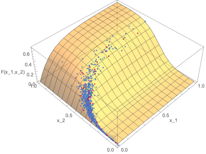
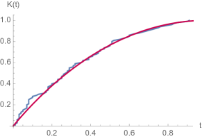
Figure 1: A bivariate distribution PDF and its corresponding Kendall statistics empirical CDF

In order to identify the sampling mechanism (step 1 of our procedure) we consider its expression (Genest and Rivest 1993):

$$u=\frac{t\left(1-t^{\alpha}+\alpha\right)}{\alpha}I_{[0,1]}(t)$$ (8)

Our strategy is to infer $\alpha$ from a sample of $T$ derived from a sample of $\{X_{1},X_{2}\}$. However, notwithstanding the simplicity of the expression (8) which depends uniquely on $\alpha$, no sufficient statistic exists for it. Hence to fulfill step 2, we decided to partition the CDF expressions so as to have two dummy distributions separately allowing a sufficient statistic whose expression is scarcely affected by the dependence between the sampled $T_{i}$s. Namely, we consider the two dummy CDFs:

$$\widetilde{K}_{1}(t)=t\frac{\alpha+1}{\alpha};\quad\quad\widetilde{K}_{2}(t)=\frac{t^{\alpha+1}}{\alpha}$$ (9)

so that $s_{1}=\sum_{i=1}^{m}t_{i}$ and $s_{2}=\sum_{i=1}^{m}\log{t_{i}}$ are respectively the sufficient statistics for $\alpha$. The instantiation of the Integral Transform Theorem to identify $g^{1}_{\alpha}$ and $g^{2}_{\alpha}$ reads as follows.

$$U=W_{1}-(W_{1}-U)=T\frac{\alpha+1}{\alpha}-\frac{T^{\alpha+1}}{\alpha}$$ (10)

where we split the seed in two with the overall aim of having the original seed $U$ facing (8) in order to accomplish step 1. From these equations we derive:

$$t=g^{1}_{\alpha}(w_{1})=w_{1}\frac{\alpha}{\alpha+1};\quad\quad t=g^{2}_{\alpha}(w_{1}-u)=\left(\alpha(w_{1}-u)\right)^{\frac{1}{\alpha+1}}$$ (11)

Equating the two right members of (11), for any sample $t_{i}$ we find the value of the second seed $w_{1}$ as a solution of the equation:

$$w_{1}\frac{\alpha}{\alpha+1}=(\alpha(w_{1}-u))^{1/(\alpha+1)}$$ (12)

as a function of $u$.

Now that the function $g_{\alpha}$ has been identified, at least in an implicit way, let us consider its seed. As previously mentioned, we are not working with independent $t_{i}$s. Thus we sample $U$ from the ECDF of $T$ CDF evaluated on the sampled $t_{i}$s. This entails a circular procedure where, starting from a tentative $\widehat{\alpha}$ – for instance its maximum likelihood estimate (MLE) – we evaluate the $w_{1i}$s so as to be able to implement steps 3 and 4 of our procedure by deriving $\widehat{\alpha}$ from the above sufficient statistics as:

$$\widehat{\alpha}_{1}=\frac{\sum_{i=1}^{m}t_{i}}{\sum_{i=1}^{m}w_{1i}-\sum_{i=1}^{m}t_{i}};\quad\widehat{\alpha}_{2}=\left\{\alpha:\sum_{i=1}^{m}\log(t_{i})=\frac{\sum_{i=1}^{m}\log(w_{1i}-u_{i})+m\log\alpha}{\alpha+1}\right\}$$ (13)

Using their mean $(\widehat{\alpha}_{1}+\widehat{\alpha}_{2})/2$ as a new instance of $\alpha$ we may recompute $w_{1i}$s until convergence.

Remark: In another paper (Apolloni and Bassis 2018) we acquainted a rather complementary inference problem on many parameters of a scalar variable distribution. In both cases we face a lack of independence on the involved statistics. The chainability property, invoked there as an antidote on the many parameters, here has a counterpart on the CDF split as in (9).

3 Implementing the bootstrap procedure

The variant of the standard procedure we discussed in the previous section presents two distinguishing features as to the identification of the seeds and to their bootstrapping. Both entail computational problems that we solved using standard tools available in a common mathematical package (Mathermatica 11.0 - Wolfram(Mathematica 2018)). We are not interested in rescaling twin CDFs in (9) to reach exactly $1$ at their right extreme, since this does not affect the sufficiency of the statistics $s_{1}$ and $s_{2}$, given the strictly monotone relationships between them and the parameter for common values of seeds and parameter. Rather, the crucial point of the procedure is the search for a fixed point for $\widehat{\alpha}$. This passes through a mean-field process consisting of iterative solutions of (12) and a rough averaging of the two separate currently estimates of $\alpha$.

To identify the problems involved, we did a set of intermediate experiments. The experimental environment is represented by the pairs $\{\alpha,m\}$ in Table 2, tossed with samples of size $50$.

$\alpha|m$	20	30	$100$
0.8	0.8 , 20	0.8 , 30	0.8 , 100
1.7	1.7 , 20	1.7 , 30	1.7 , 100
3	3 , 20	3 , 30	3 , 100
5	5 , 20	5 , 30	5 , 100

Table 2: The experimental plan. $\alpha\rightarrow$ target Clayton parameter; $m\rightarrow$ size of the sample processed by the estimators.

3.1 The parameter distribution

First, we use exactly $\alpha$ and $m$ to generate both:

1. the $50$ samples $(\{u_{1,i},u{{}_{2},i}$ with $i\in\{1,\ldots,m\})$from $CDF|u_{1}$ in Table 1 , $t_{i}$s from (2) and related statistics $(s_{1}=\sum t_{i},s_{2}=\sum\log(t_{i})$, and

2. for each sample a bootstrap population of $300$ replicas of $m$ seeds $\{w_{1},u-w_{1}\}$ from(12) .

From these exact seeds we compute on each sample the estimate $\hat{\alpha}=(\hat{\alpha}_{1}+\hat{\alpha}_{2})/2$, so as to have 50 parameter populations of $300$ estimates on each cell of Table 2. While Figure 2 reports a short excerpt of them, Table 3 reports for each experimental cell the mean and standard deviation of the distribution central values. We contrast these values with the MLEs on the same $50$ samples on each cell, where MLE is directly computed by numerically maximizing the product of the$t_{i}$ instantiations of Kendall PDF reported in Table 1. As customary in the AI approach, central values are represented by the medians of our estimators, contrasted with the single MLEs. We may see that our estimators generally outperform the MLE companion.

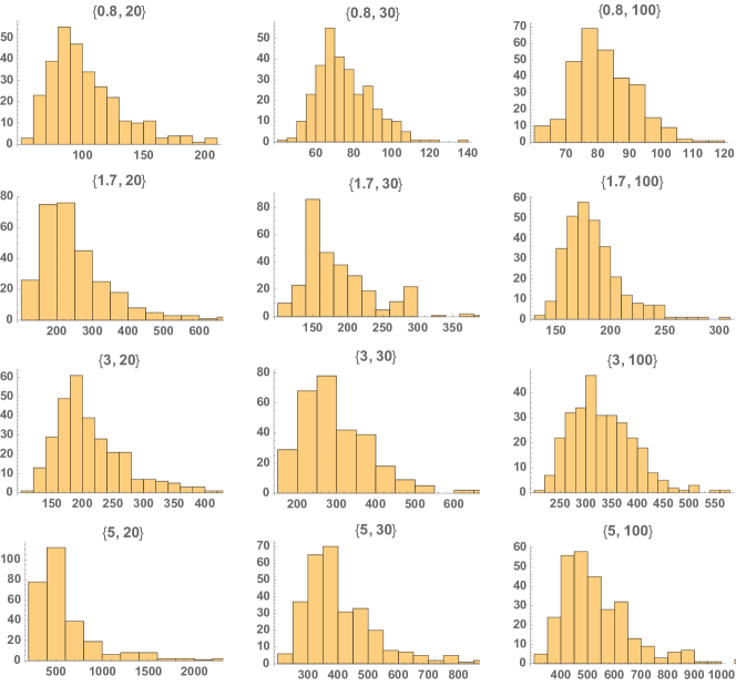
Figure 2: An excerpt of the parameter distributions. The histograms refer to the value of the parameters times 100.

$\alpha$	statistic	$\alpha_{\mathrm{AI}}$	$\alpha_{\mathrm{MLE}}$	$\alpha_{\mathrm{AI}}$	$\alpha_{\mathrm{MLE}}$	$\alpha_{\mathrm{AI}}$	$\alpha_{\mathrm{MLE}}$
		m=	20	m=	30	m=	100
0.8	mean	0.758288	1.9211	0.756991	1.30998	0.794989	0.974008
	stdv	0.0867599	1.39259	0.0426901	0.805682	0.046596	0.266865
1,7	mean	1.57008	3.2841	1.62256	2.45001	1.68961	1.99565
	stdv	0.110117	2.53951	0.109423	0.893306	0.080659	0.47425
3	mean	2.72937	6.1436	2.84787	4.80562	2.89506	3.26851
	stdv	0.247745	5.7625	0.222166	3.17289	0.185544	0.808644
5	mean	4.42341	8.91136	4.48985	9.16353	4.7606	5.74891
	stdv	0.414849	7.69919	0.4082	8.90931	0.267965	1.78936

Table 3: Comparison between a dummy version of the proposed estimator $\alpha_{\mathrm{AI}}$ and maximum likelihood companion $\alpha_{\mathrm{MLE}}$ computed on $50$ samples for each instance of the experimental plan. Cells: estimates’ mean and standard deviation.

3.2 The estimator distribution

As mentioned before, we have no true $\alpha$ to draw the seeds $\{w_{1},u-w_{1}\}$, hence we must replay it with an estimator within a circular procedure. We devote the first $300$ steps of the procedure to approach a fixed point $\alpha$ and another $300$ steps to collect a local distribution of $\hat{\alpha}$, whose median is used as the final estimator. Like the previous experiment, we compute this estimator on $50$ samples $(\{u_{1,i},u_{2,i}$ with $i\in\{1,\ldots,m\})$. On these vales we compute the same statistics as in the previous experiment, which we may see in Table 4.

$\alpha$	statistic	$\alpha_{\mathrm{AI}}$	$\alpha_{\mathrm{MLE}}$	$\alpha_{\mathrm{AI}}$	$\alpha_{\mathrm{MLE}}$	$\alpha_{\mathrm{AI}}$	$\alpha_{\mathrm{MLE}}$
		m=	20	m=	30	m=	100
0.8	mean	1.1177	1.93252	0.815224	1.30876	0.792833	0.944016
	stdv	0.694839	1.20238	0.43988	0.506298	0.196159	0.229342
1.7	mean	2.34081	2.81598	1.76855	2.32431	1.71466	1.87771
	stdv	1.87018	2.18893	0.956257	1.2762	0.358178	0.370696
3	mean	4.95876	7.15575	4.18669	5.26361	3.06338	3.28108
	stdv	2.41092	11.689	2.10042	6.02015	0.606473	0.737848
5	mean	7.01755	7.54718	6.30799	9.30124	5.66863	5.84041
	stdv	2.59534	10.8293	1.37502	8.90931	1.00474	1.7298

Table 4: Comparison between the proposed estimator $\alpha_{\mathrm{AI}}$ and maximum likelihood companion $\alpha_{\mathrm{MLE}}$. Same notation as in Table 3.

Since the initial value of $\hat{\alpha}$ coincides with the MLE on the same sample, this accounts for checking whether further computations improve the estimations or not. Though the actual estimators are less approximate than the dummy ones reported in the previous table, the edge of our procedure re MLE definitely remains as for both central values and dispersions. In the next section we will elaborate on this edge.

4 Discussion

Willing to explore the capability of our approach on the base problem of estimating the parameter $\alpha$ of the bivariate Clayton copulas, we leave to other papers (Apolloni et al. (2006, 2009); Apolloni and Bassis (2011)) the task of showing the comparative benefits and different semantics of AI approach re more assessed ones in the literature. Rather, in this section we constrain the discussion inside the AI approach itself to appreciate the gain of further elaborations on data beyond the computation of the maximum likelihood, as for point estimators. We also show our own implementation of the confidence intervals for $\alpha$ and make considerations on the generality of the proposed method.

4.1 Point Estimates

A comparison between Tables 3 and  4 highlights the drawback deriving from using an estimate of $\alpha$ in place of its true value during the generation of the pairs $\{w_{1},u-w1\}$. This, in turn, derives from the bias of $\hat{\alpha}$. Actually, there is no great spread between $\alpha_{1}$ and $\alpha_{2}$ (see Figure 3 for a typical example of joint trajectories along a cycle).

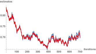
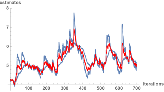
Figure 3: Two mean-field convergence instances in the cells $(\alpha=0.8,m=20)$ and $(\alpha=5,m=100)$, respectively. Red path $\rightarrow\alpha_{1}$, blue path $\rightarrow\alpha_{2}$.

Rather, the trajectories are banding, notwithstanding a low-coefficient-exponential smoothing adopted to constrain the oscillations, with the chance of being attracted by local minima, especially for high vales of $m$. Note that, MLEs too are spreading with respect to the target parameter, with the same trend re $m$. And, since these estimators are the starting point in the search for the $\hat{\alpha}$ fixed point, MLE drifts generally induce analogous $\hat{\alpha}$ drifts. Nonetheless, the mean-field trajectories generally get closer than MLE’s to the target. This is stemmed by the individual corrections induced by the mean-field process on the original MLE, as shown in Figure 4. While for $\alpha=0.8$ we see a general bias toward lower values, with $\alpha=5$ the correction is more selective, by inducing generally a positive shift in case of MLE underestimate and negative ones in the opposite case.

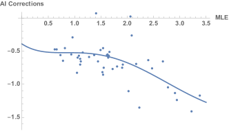
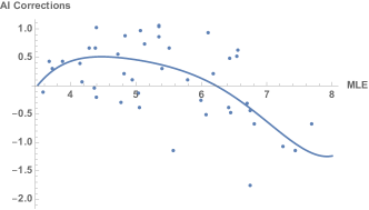
Figure 4: The mean-field corrections in the cells $(\alpha=0.8,m=20)$ and $(\alpha=5,m=100)$, respectively. Continuous curve $\rightarrow$ fifth order fit.

As a result, we have a more favorable distribution of the estimates with our method. See Figure 5 for a pair of instances. AI estimators are generally less biased and less dispersed. The biases are normally positive.

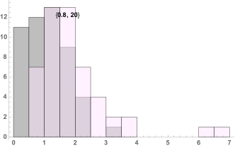
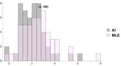
Figure 5: Comparison of the histograms of the AI and MLE estimators in two typical instances.

4.2 Interval Estimates

Looking at the distribution of the $\hat{\alpha}$ replicas of our estimators we see non trivial empirical distributions (see Figure 6-left for instance) that can be used to compute confidence intervals for $\alpha$, yet avoiding to enforce an asymptotic distribution approximation (normal, $\chi^{2}$, etc.) (Chen et al. 2009; Peng and Ruodu 2014; Hofert et al. 2012). Namely, in the Algorithmic Inference framework we draw replicas of parameter estimates from replicas of their random seeds. By transferring the probability masses from the latter to the former, we obtain an empirical distribution of the random parameter that is compatible with the observed sample (Apolloni et al. 2009), as in Figure 6-right.

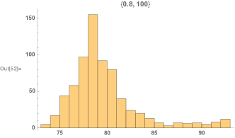
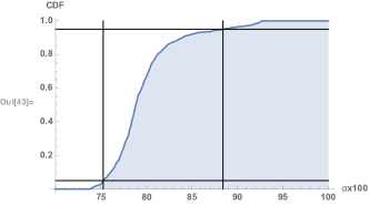
Figure 6: From the histogram of the estimators for a given sample (left picture) to the quantiles identifying the confidence interval (right picture). To gain details, the estimate values are multiplied by $100$.

Two expedients are necessary in order to get satisfactory intervals by-passing two drawbacks in the statistic, respectively.

1. Actually, assuming $\hat{\alpha}$ to be stabilized after a certain number of iterations, we could use the further tail of the mean-field process to draw $\alpha$ distribution. However, the continuous $\hat{\alpha}$ updating, and plus using the exponential smoothing, make the statistics highly correlated. Hence our strategy has been to exploit the tail to compute a reliable estimate $\tilde{\alpha}$ as the median of the tail values, to obtain a population of new estimates putting $\tilde{\alpha}$ in (6) in analogy to what we did in section 3.1.

2. Once the parameter distribution has been obtained, any confidence interval may be delimited by the proper quantiles of this distribution. However, in turn, the population of the new estimates suffers from the fact that the seeds $\{w_{1,i},u_{i}-w_{1,i}\}$ are based on $\tilde{\alpha}$ that is an approximation of the original value $\alpha$. This may entail hard shifts among the confidence intervals, which we reduce simply by computing the quantiles on the merging of three consecutive empirical distributions (within the $50$ ones available on each cell). Figure 7 shows the good coverage of the $48$ intervals that are obtained in this way for each cell, where the adopted quantiles are at levels $(0.05,0.95)$.

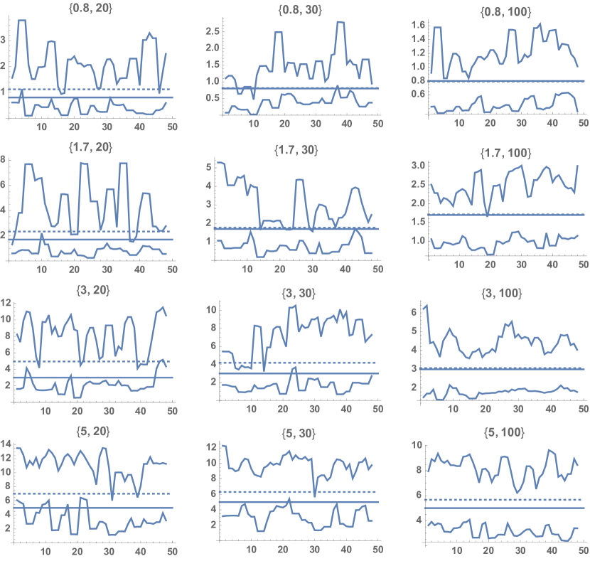
Figure 7: Trends of the upper-bounds and lower-bounds of the $0.9$ confidence intervals with the samples in the various cells. Straight lines: continuous line $\rightarrow$ original $\alpha$, dotted line estimated $\tilde{\alpha}$.

4.3 Procedure Extendability

In conclusion, we may establish a clear benefit deriving from our procedure. However, looking at the expressions of $T$ CDFs in Table 5 we realize that only the Clayton and Gumbel copulas are easily separable as in (9). Thus we expect to find some difficulties in extending this procedure to other families of copulas.

Family	$\phi(v)$	$K(v)$
Clayton	$\frac{v^{-\alpha-1}}{\alpha}$	$\frac{v(1-v^{\alpha}+\alpha)}{\alpha}$
Gumbel	$(-\log v)^{\alpha+1}$	$\frac{v(1-\log v)}{\alpha+1}$
Frank	$\log\frac{1-\mathrm{e}^{-\alpha}}{1-\mathrm{e}^{-\alpha v}}$	$v+\frac{1-\mathrm{e}^{-\alpha v}}{\alpha\mathrm{e}^{-\alpha v}}\log\frac{1-\mathrm{e}^{-\alpha}}{1-\mathrm{e}^{-\alpha v}}$
Joe	$-\log(1-(1-v)^{\alpha})$	$v-\frac{\left(1-(1-v)^{\alpha}\right)(1-v)^{1-\alpha}\log\left(1-(1-v)^{\alpha}\right)}{\alpha}$
Ali-Mikhail-Haq	$\log\left(\frac{\alpha v-\alpha+1}{v}\right)$	$v-\frac{(\alpha-1)\log\left(\frac{\alpha(v-1)+1}{v}\right)}{v(\alpha(v-1)+1)}$

Table 5: Excerpt of Archimedean copula families with generator $\phi(v)$ and Kendall’s function $K(v)$.

5 Conclusions

In this paper we use Algorithmic inference methods to solve the crucial problem of estimating the parameter $\alpha$ of the bivariate Clayton copulas. This task is relevant in two respects:

• from a functional perspective it is the gateway for dealing with many dependency estimates.

• from a statistical perspective, the solution requires the engagement of non trivial algorithms to compute the estimators.

The second aspect frequently occurs in Computational Intelligence instances. The Algorithmic Inference framework faces it by explicitly exploiting the connections between the computational and probabilistic properties of statistics. In this way, we don’t elude the computational burden of other inference methods such as MLE. Rather, we better finalize it to obtain functions that suitably transfer the statistical features of a sample to the statistical properties of an unknown parameter. This passes through the identification of an ECDF of $\alpha$ that allows for suitable both point and by interval estimators. Thanks to the numerical strategies discussed in this paper, the numerical results show that this approach provides comparative benefits that are tangible in both kinds of estimates.

References

Funding

This research did not receive any specific grant from funding agencies in the public, commercial, or not-for-profit sectors.

References

- Apolloni and Bassis (2011) Apolloni, B. and S. Bassis (2011). Confidence about possible explanations. IEEE Transactions on Systems, Man, and Cybernetics, Part B: Cybernetics 41(6), 1639–1653.
- Apolloni and Bassis (2018) Apolloni, B. and S. Bassis (2018). The randomness of the inferred parameters. a machine learning framework for computing confidence regions. Information Sciences 453, 239 – 262.
- Apolloni et al. (2009) Apolloni, B., S. Bassis, and D. Malchiodi (2009). Compatible worlds. Nonlinear Analysis: Theory, Methods & Applications 71(12), e2883–e2901.
- Apolloni et al. (2008) Apolloni, B., S. Bassis, D. Malchiodi, and W. Pedrycz (2008). The Puzzle of Granular Computing, Volume 138 of Studies in Computational Intelligence. Springer Verlag.
- Apolloni et al. (2006) Apolloni, B., D. Malchiodi, and S. Gaito (2006). Algorithmic Inference in Machine Learning, 2nd Edition. International Series on Advanced Intelligence, Vol. 5. Magill, Adelaide: Advanced Knowledge International.
- blog copulas (2011) blog copulas (2011). Algorithmic Inference approach to learn copulas. http://www.probabilistic-numerics.org/apollonietal.pdf.
- Brechmann and Schepsmeier (2013) Brechmann, E. and U. Schepsmeier (2013). Modeling dependence with c- and d-vine copulas: The r package cdvine. Journal of Statistical Software, Articles 52(3), 1–27.
- Bücher and Volgushev (2013) Bücher, A. and S. Volgushev (2013). Empirical and sequential empirical copula processes under serial dependence. Journal of Multivariate Analysis 119, 61 – 70.
- Chen et al. (2009) Chen, J., L. Peng, and Y. Zhao (2009). Empirical likelihood based confidence intervals for copulas. Journal of Multivariate Analysis 100(1), 137 – 151.
- Coolen-Maturi et al. (2016) Coolen-Maturi, T., F. P. A. Coolen, and N. Muhammad (2016). Predictive inference for bivariate data: Combining nonparametric predictive inference for marginals with an estimated copula. Journal of Statistical Theory and Practice 10(3), 515–538.
- Genest et al. (2011) Genest, C., J. Neslehova, and J. Ziegel (2011). Inference in multivariate archimedean copula models. TEST 20, 223–256.
- Genest and Rivest (1993) Genest, C. and L. Rivest (1993). Statistical inference procedures for bivariate archimedean copulas. Journal of the American Statistical Association 88, 1034–1043.
- Genest and Segers (2009) Genest, C. and J. Segers (2009). Rank-based inference for bivariate extreme-value copulas. The Annals of Statistics 37(5B), 2990–3022.
- Hofert et al. (2012) Hofert, M., M. Mächler, and A. McNeil (2012). Likelihood inference for archimedean copulas in high dimensions under known margins. Journal of Multivariate Analysis 110, 133 – 150. Special Issue on Copula Modeling and Dependence.
- Mathematica (2018) Mathematica, w. (2018). Mathematica 11. http://www.wolfram.com.
- McNeil and Neslehova (2009) McNeil, A. J. and J. Neslehova (2009). Multivariate archimedean copulas, d-monotone functions and l1-norm symmetric distributions. Annals of Statistics 37(5b), 3059–3097.
- Peng and Ruodu (2014) Peng, L. and W. Ruodu (2014). Interval estimation for bivariate t-copulas via kendall s tau. Variance 8(1), 43–54.
- Rohatgi (1976) Rohatgi, V. K. (1976). An Introduction to Probablity Theory and Mathematical Statistics. Wiley Series in Probability and Mathematical Statistics. New York: John Wiley & Sons.
- Sklar (1973) Sklar, A. (1973). Random variables, joint distribution functions, and copulas. Kybernetika 9(6), 449–460.