Effective Stabilized Self-Training on Few-Labeled Graph Data

Abstract

Graph neural networks (GNNs) are designed for semi-supervised node classification on graphs where only a subset of nodes have class labels. However, under extreme cases when very few labels are available (e.g., 1 labeled node per class), GNNs suffer from severe performance degradation. Specifically, we observe that existing GNNs suffer from unstable training process on few-labeled graphs, resulting to inferior performance on node classification. Therefore, we propose an effective framework, Stabilized Self-Training (SST), which is applicable to existing GNNs to handle the scarcity of labeled data, and consequently, boost classification accuracy. We conduct thorough empirical and theoretical analysis to support our findings and motivate the algorithmic designs in SST. We apply SST to two popular GNN models GCN and DAGNN, to get SSTGCN and SSTDA methods respectively, and evaluate the two methods against 10 competitors over 5 benchmarking datasets. Extensive experiments show that the proposed SST framework is highly effective, especially when few labeled data are available. Our methods achieve superior performance under almost all settings over all datasets. For instance, on a Cora dataset with only 1 labeled node per class, the accuracy of SSTGCN is $62.5\%$, $17.9\%$ higher than GCN, and the accuracy of SSTDA is $66.4\%$, which outperforms DAGNN by $6.6\%$.

Conduct thorough analysis on node classification over few-labeled graphs

Propose a stabilized self-training framework to improve performance

Evaluate the performance of proposed methods on real graph data

1 Introduction

A graph models the relationships between objects as the edges between nodes. Graphs are ubiquitous with a wide range of real-world applications, e.g., social network analysis [1, 2], traffic prediction [3], protein interface prediction [4], and recommendation systems [5, 6]. An important task to support these applications is node classification that aims to classify the nodes in a graph into various classes. However, effective node classification is challenging, especially due to the lack of sufficient labeled data that are expensive to obtain.

To mitigate the issue, semi-supervised node classification on graphs has attracted much attention [7, 8]. It leverages a small amount of labeled nodes as well as the unlabeled nodes in a graph to train an accurate classification model. There exists a collection of Graph Neural Networks (GNNs) for semi-supervised node classification [7, 8, 9, 10]. For instance, Graph convolution networks (GCNs) rely on a message passing scheme via graph convolution operations to aggregate the neighborhood information of a node to generate node representation, which can then be used in downstream classification tasks. Despite the great success of GCNs, under the extreme cases when very few labels are given (e.g., only 1 labeled node per class), the shallow GCN architecture, typically with two layers, cannot effectively propagate the training labels over the input graph, leading to inferior performance as shown in the experiments (Tables 3, 4 and 5). Recently, several studies try to improve classification accuracy by designing deeper GNN architectures, e.g., DAGNN [7]. However, deep GNNs are still not directly designed to tackle the scarcity of labeled data.

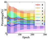
(a) GCN

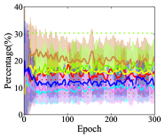
(b) DAGNN

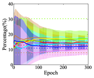
(c) SSTGCN

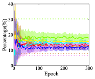
(d) SSTDA

Figure 1: The distribution of predicted labels in different classes in Cora-$1$.

After conducting an in-depth study, we have an interesting finding that existing GNNs suffer from an issue of unstable training, when labeled nodes are few. In particular, on a Cora dataset with 7 classes (see Section 5 for dataset details), for each run, we randomly select 1 labeled node per class as the training data (denoted as Cora-1). Then on Cora-1, we run GCN and DAGNN 100 times with 300 epochs per run, and get the average number of predicted labels per class with standard deviation at every epoch in percentage. The statistical results of GCN and DAGNN are shown in Figures 1(a) and 1(b) respectively, where $x$-axis is the epoch from 0 to 300, and $y$-axis is the percentage of a class in the predicted node labels. There are 7 colored curves representing the average percentage of the predicted labels of the respective classes. The dashed straight lines are the ground-truth percentage of every class in the Cora dataset. The shaded areas in color represent the standard deviation. Observe that in Figure 1(a), GCN has high variance at different runs when predicting node labels, and the variance keeps large at late epochs, e.g., 300, which indicates that GCN is quite unstable at different runs with 1 training label per class sampled randomly, leading to inferior classification accuracy as illustrated in our experiments. As shown in Figure 1(b), DAGNN also suffers from the issue of unstable training. The variance of DAGNN is relatively smaller than that of GCN, which provides a hint why DAGNN performs better than GCN. Nevertheless, both GCN and DAGNN yield unstable training process with large variance. Since there is only 1 labeled node per class for training, the randomly sampled training nodes can heavily influence the message passing process in GCN and DAGNN, depending on the connectivity of the training nodes to their neighborhoods over the graph topology, which result to the unstable training process observed above. In literature, there exists a collection of self-training techniques that enhance the training data by using predicted labels as pseudo labels for training [11, 12]. However, as identified in our empirical analysis in Section 4.1, these methods generate imbalanced pseudo labels, which could affect the performance.

To address the above issues when few labeled data are available, we propose a Stabilized Self-Training (SST) framework, which is readily applicable to existing GNNs to improve classification accuracy via stabilized training process. We first conduct thorough empirical and theoretical analysis to identify and explain the issues of existing methods when trained with few labeled nodes for classification. Motivated by the analysis, in the proposed SST framework, we select a set of nodes with predicted labels of high confidence as high-quality pseudo labels, and add such pseudo labels into training data to enhance the training of next epoch, while filtering out the low-confidence predicted labels. To tackle the unstable training issue of existing GNNs, we develop a stabilized pseudo labeling technique to balance the importance of different classes in training. We then design a negative sampling regularization technique over pseudo labels to further improve node classification accuracy. In experiments, we apply our SST framework to GCN and DAGNN to get methods SSTGCN and SSTDA respectively. Figures 1(c) and 1(d) report the average percentage and standard variance of the predicted labels per class per epoch of SSTGCN and SSTDA on Cora-1 respectively. Compared with Figure 1(a) of GCN, obviously, the variance of SSTGCN in Figure 1(c) decreases quickly and becomes stable as epoch increases. SSTDA is also more stable than DAGNN, as shown in Figures 1(d) and 1(b) respectively. We conduct extensive experiments on 5 benchmarking datasets, and compare with 10 existing solutions, to evaluate the performance of the proposed SST framework. Experimental results demonstrate that SST is able to significantly improve classification accuracy of existing GNNs when only few labels are available. For instance, with the proposed SST framework, SSTGCN achieves $62.5\%$ node classification accuracy on Cora-1, significantly improving GCN ($44.6\%$) by $17.9\%$, and SSTDA obtains $66.4\%$ accuracy on Cora-1 and outperforms DAGNN ($59.8\%$) by a substantial margin of $6.6\%$.

In summary, our main contributions are as follows:

• We conduct thorough empirical and theoretical analysis, and make important findings that existing GNNs are unstable when training with few-labeled graph data, and existing self-training techniques suffer from low-quality and imbalanced pseudo labels. Our theoretical analysis provides solid explanations for the findings.

• We present a Stabilized Self-Training (SST) framework that can significantly improve classification performance by stabilizing the training process of GNNs. Based on our analysis, SST consists of a stabilized pseudo labeling technique and a negative sampling regularization technique over pseudo labels.

• We apply SST to popular GNNs, and conduct extensive experiments on 5 datasets to compare against 10 existing methods. The experimental results demonstrate the superior performance of our proposed techniques.

The rest of the paper is organized as follows. We review the related work in Section 2. In Section 3, we present the problem formulation of semi-supervised node classification on few-labeled graph data. We present our analysis and method in Section 4. In particular, we present the empirical analysis in Section 4.1, conduct theoretical analysis in Section 4.2, and then develop the SST framework in Section 4.3. Extensive experiments are reported in Section 5. Finally, we conclude the paper in Section 6. All proofs are in A.

2 Related Work

In literature, there are two directions to address the scarcity of labeled data for semi-supervised node classification: (i) explore multi-hop graph topological features to propagate the training labels over the input graph [9, 7]; (ii) enhance the labeled data by self-training and pseudo labeling [11, 13]. Note that these two directions are not mutually exclusive, and they can be applied together on few-labeled graph data. Here we review the existing studies that are most relevant to this paper.

There exist a large collection of GNNs [7, 8, 9, 14, 15, 16, 17, 18]. We introduce the details of GCN [9] and DAGNN [7] here. GCN learns the representation of each node by iteratively aggregating the representations of its neighbors. Specifically, GCN consists of $k$ layers, each with the same propagation rule defined as follows. At the $\ell$-th layer, the hidden representations $\mathbf{H}^{(\ell-1)}$ of previous layer are aggregated to get $\mathbf{H}^{(\ell)}$,

$$\mathbf{H}^{(\ell)}=\sigma(\hat{\mathbf{A}}\mathbf{H}^{(\ell-1)}\mathbf{W}^{(\ell)}),\ell=1,2,...,k.$$ (1)

$\hat{\mathbf{A}}=\tilde{\mathbf{D}}^{-\frac{1}{2}}\tilde{\mathbf{A}}\tilde{\mathbf{D}}^{-\frac{1}{2}}$ is the graph laplacian, where $\tilde{\mathbf{A}}=\mathbf{A}+\mathbf{I}$ is the adjacency matrix of $\mathcal{G}$ after adding self-loops ($\mathbf{I}$ is the identity matrix) and $\tilde{\mathbf{D}}$ is a diagonal matrix with $\tilde{\mathbf{D}}_{ii}=\sum_{j}\tilde{\mathbf{A}}_{ij}$. $\mathbf{W}^{(\ell)}$ is a trainable weight matrix of the $\ell$-th layer, and $\sigma$ is a nonlinear activation function. Initially, $\mathbf{H}^{(0)}=\mathbf{X}$, where $\mathbf{X}$ is the input feature matrix, describing the node features of all nodes in the input graph. Note that GCN usually achieves superior performance with 1 layer or 2 layers. When applying many layers to explore large receptive fields, GCN yields degraded performance, due to the over-smoothing issue [11, 19, 20]. DAGNN addresses the over-smoothing issue by decoupling representation transformation and propagation in GNNs [7]. Then it utilizes an adaptive adjustment mechanism to balance the information from local and global neighborhoods of every node. Specifically, the mathematical expression of DAGNN is as follows. DAGNN uses a learnable parameter $\mathbf{s}\in^{c\times 1}$ to adjust the weight of embeddings at different propagation level (from $1$ to $k$).

$$\mathbf{Z}= \text{MLP}(\mathbf{X})\in^{n\times c}$$

$$\mathbf{H}_{\ell}= \hat{\mathbf{A}}^{\ell}\cdot\mathbf{Z}\in^{n\times c},\ell=1,2,...,k$$

$$\mathbf{S}_{\ell}= \mathbf{H}_{\ell}\cdot\mathbf{s}\in^{n\times 1},\ell=1,2,...,k$$

$$\hat{\mathbf{S}}_{\ell}= [\mathbf{S}_{\ell},\mathbf{S}_{\ell},...,\mathbf{S}_{\ell}]\in^{n\times c},\ell=1,2,...,k$$

$$\mathbf{X}_{out}= \text{softmax}(\sum_{\ell=1}^{k}\mathbf{H}_{\ell}\odot\hat{\mathbf{S}}_{\ell}),$$

where $\hat{\mathbf{A}}^{\ell}$ is the $\ell$-th power of matrix $\hat{\mathbf{A}}$, $\odot$ is the Hadamard product, $\cdot$ is dot product, MLP is the Multilayer Perceptron and softmax operation is on the second dimension.

Apart from GCN and DAGNN, initial GNN studies apply convolution operation in the spectral domain, where the eigenvectors of the graph Laplacian are considered as the Fourier basis [21, 22]. Then GAT [14] assigns different weights to nodes in the same neighborhood via attention mechanisms. Monti et al. [15] define convolutions directly in the spatial domain using mixture model CNNs. APPNP [8] adopts a propagation rule based on personalized PageRank [23], so as to gather both local and global information on graphs. GpLCN [18] utilizes the manifold structure information by p-Laplacian matrix to extract abundant features for classification. As evaluated in experiments, existing methods yield inferior performance [7, 8, 9, 14], since they are not directly designed to tackle the scarcity of labeled data.

As previously mentioned, another way to address the situation of limited labeled data is to add pseudo labels to training dataset by self-training [11]. Self-training is a general methodology [24] used in various applications. Zhou et al. [25] suggest that selecting informative unlabeled data using a guided search algorithm can significantly improve performance over standard self-training framework. Buchnik and Cohen [26] mainly consider self-training for diffusion-based techniques. Recently, self-training has been adopted for semi-supervised tasks on graphs. For instance, Li et al. [11] propose self-training and co-training techniques for GCN. This self-training work selects the top-$k$ confident predicted labels as pseudo labels. Co-training technique co-trains a GCN with a random walk model to handle few-labeled data [11, 27]. Sun et al. [12] utilize a DeepCluster technique to refine the selected pseudo labels. Compared with existing self-training methods, our framework is different. In particular, our framework has a different strategy to select pseudo labels and also has a stabilizer to address the deficiencies of existing GNNs. Moreover, we propose a negative sampling regularization technique to further boost accuracy. Besides, in existing work, if a node is selected as a pseudo label, it will never be moved out even if the pseudo label becomes obviously wrong in later epochs. On the other hand, in our framework, we update pseudo labels in each epoch to avoid such an issue. A recent work [28] further takes node informativeness into account for pseudo-label selection.

Further, there are extensive studies on network embedding in recent years, which aims to learn a low-dimensional embedding vector per node in an unsupervised manner [29, 30, 31, 32]. The learned embedding vectors can be then used in downstream tasks, including node classification. Perozzi et al. [29] use truncated random walks to learn latent representations, with the assumption that nodes are similar if they are close by random walks. Tang et al. [30] propose to preserve and concatenate the first-order and second-order proximity representations between nodes. G2G [31] embeds each node as a Gaussian distribution according to a ranking similarity based on the shortest path distances between nodes. DGI [32] is an embedding method based on GCNs with unsupervised objective that is to maximize mutual information between patch representations and corresponding high-level summaries of graphs. However, these unsupervised methods do not leverage labeled data, and thus are not as accurate as our methods in experiments.

3 Preliminaries

Let $\mathcal{G}=(\mathcal{V},\mathcal{E},\mathbf{X})$ be a graph consisting of a node set $\mathcal{V}$ with cardinality $n$, a set of edges $\mathcal{E}$ of size $m$, and a feature matrix $\mathbf{X}\in^{n\times d}$, where $d$ is the number of features. An edge in $\mathcal{E}$ connects two nodes in $\mathcal{V}$. Every node $v_{i}\in\mathcal{V}$ has a feature vector $\mathbf{X}_{i}$ that is the $i$-th row of $\mathbf{X}$. Let scalar $c$ be the number of classes, and $\mathcal{C}$ be the set of class labels ($c=|\mathcal{C}|$). We use $\mathcal{L}$ to denote the set of labeled nodes, and obviously $\mathcal{L}\subseteq\mathcal{V}$. Let $\mathcal{U}$ be the set of unlabeled nodes and $\mathcal{U}=\mathcal{V}\setminus\mathcal{L}$. Each labeled node $v_{i}\in\mathcal{L}$ has a one-hot vector $\mathbf{Y}_{i}\in\{0,1\}^{c}$, indicating the class label of $v_{i}$. Under the few-labeled setting, $|\mathcal{L}|\ll|\mathcal{U}|$. The definition of the semi-supervised node classification problem is as follows.

Definition 1.

Given a graph $\mathcal{G}=(\mathcal{V},\mathcal{E},\mathbf{X})$, a set of labeled nodes $\mathcal{L}\subseteq\mathcal{V}$, and a ground-truth class label $\mathbf{Y}_{i}\in\{0,1\}^{c}$ per node $v_{i}\in\mathcal{L}$, assuming that each node belongs to exactly one class, Semi-Supervised Node Classification predicts the labels of the unlabeled nodes.

In particular, the aim is to leverage a graph $\mathcal{G}$ with the labeled nodes in $\mathcal{L}$ to train a classification model/function $f(\mathcal{G},\theta)$. The model $f$ with trainable parameters $\theta$ outputs a matrix $\mathbf{F}\in^{n\times c}$. The $i$-th row $\mathbf{F}_{i}\in[0,1]^{c}$ represents the probability vector of node $v_{i}\in\mathcal{V}$. We adopt the popular cross-entropy loss to train the model. Given a node $v_{i}$, its loss $L(\mathbf{Y}_{i},\mathbf{F}_{i})$ of $\mathbf{F}_{i}$ with respect to its true class label $\mathbf{Y}_{i}$ is

$$L(\mathbf{Y}_{i},\mathbf{F}_{i})=-\sum_{j=1}^{c}\mathbf{Y}_{i,j}\ln(\mathbf{F}_{i,j}),$$

where $\mathbf{Y}_{i,j}$ is the $j$-th value in $\mathbf{Y}_{i}$ and $\mathbf{F}_{i,j}$ is the $j$-th value in $\mathbf{F}_{i}$.

During the training process, at a certain epoch, given the matrix $\mathbf{F}$, let $\tilde{\mathbf{Y}}_{i,j}$ satisfying Eq. (2) be the predicted label of node $v_{i}$ at the epoch. In particular, if $\mathbf{F}_{i,j}$ is the largest element in vector $\mathbf{F}_{i}$, $\tilde{\mathbf{Y}}_{i,j}$ is 1, otherwise, 0. We say that, with confidence $\mathbf{F}_{i,j}$, node $v_{i}$ has class label $\mathcal{C}_{j}$.

$$\tilde{\mathbf{Y}}_{i,j}=\begin{cases}1&\text{if $j=\mathop{\arg\max}_{j^{\prime}}\mathbf{F}_{i,j^{\prime}}$},\\ 0&\text{otherwise},\end{cases}$$ (2)

4 Our Method and Analysis

We first conduct empirical analysis in Section 4.1 to identify the issues of existing techniques, and then perform theoretical analysis in Section 4.2 to reveal the latent reasons of the empirical findings. Lastly, we present our technical designs of Stabilized Self-Training (SST) in Section 4.3.

4.1 Empirical Analysis

We conduct empirical analysis to reveal that existing techniques suffer from imbalanced and low-confidence pseudo labels during the training stage. We first verify that during the training process, nodes with higher confidence tend to be predicted more accurately. On the Cora dataset with 7 classes, each with 1 labeled node for training, Figure 2a exhibits the positive correlation between the confidence and the accuracy scores of GCN at the 100-th training epoch with confidence interval 0.1. In particular, for each confidence interval ($x$-axis), we report the percentage of unlabeled nodes with predicted labels matching their ground-truth labels (i.e., accuracy in $y$-axis). Obviously, as the confidence becomes higher, the accuracy increases. On the other hand, if a method generates predictions with low confidence, its performance tends to be inferior.

(a) Confidence v.s., accuracy correlation

(b) Predicted label distribution

Figure 2: Training GCN on Cora with 1 labeled node per class (Cora-1)

(a) Early epoch: 20

(b) Middle epoch:100

(c) Late epoch: 500

Figure 3: Confidence distributions of GCN Training on Cora-1.

Then in Figure 3, we provide empirical evidence that most nodes are with low confidence, especially at the early epochs of the training, which will hamper the performance. Specifically, in Figures 3a, 3b, and 3c, we illustrate the distributions of the confidence scores of all nodes in unlabeled set $\mathcal{U}$ on Cora, at early (20-th), middle (100-th), and late (500-th) epochs, respectively. Observe that at the early epoch in Figure 3a, $95.4\%$ of the unlabeled nodes are with very low confidence ($<0.2$). If pseudo labels are generated based on the low confidences at early epochs, then such pseudo labels are inaccurate as verified above. Subsequently, they will severely influence the training of later epochs, resulting to unstable training process and unexpected performance degradation. Further, low-confidence nodes are still the majority during middle epochs, e.g., 100-th epoch in Figure 3b. The number of low-confidence nodes decreases significantly at very late epochs, e.g., 500-th epoch in Figure 3c. These observations indicate that the low-confidence nodes keep exposing significant influence during the major part of the whole training process.

Further, Figure 2b shows the distribution of the predicted labels of the nodes in $\mathcal{U}$ at the 20-th epoch on Cora in a single run. Obviously, the distribution of the labels is highly imbalanced, i.e., $92.4\%$ of the nodes are with class 1 and $6.6\%$ are with class 4. The imbalanced class labels (i.e., class 1 in Figure 2b) will heavily affect the direction of gradient descent during the training process, imposing the model to learn weights resulting to imbalanced predictions, which is often not the ground-truth case. If too many low-confidence nodes are wrongly assigned to a single class at early epochs, existing GNNs, such as GCN, which rely on propagation and transformation over graph topology, will suffer from unstable performance as reported in Figure 1.

4.2 Theoretical Analysis

The semi-supervised node classification problem studied in this paper naturally fits the transductive learning setting, since all labeled and unlabeled data in the input graph $\mathcal{G}$ are known, and no more new data will be added [33]. In the following, we analyze the problem from the perspective of gradient descent, to theoretically explain the findings made in Section 4.1.

Under the ideal case where we have the labels of all nodes in $\mathcal{V}$ (the population), given a classifier $f(\mathcal{G},\theta)$ with output probability vectors $\mathbf{F}_{i}$ for all nodes $v_{i}$ in $\mathcal{V}$, the population loss $L_{pop}$ is computed as follows. Ideally, the objective is to minimize $L_{pop}$ by evaluating population gradient $\nabla_{\theta}L_{pop}$, and find optimal parameters $\theta^{*}$.

$$L_{pop}=\mathbb{E}_{v_{i}\sim\mathrm{U}(\mathcal{V})}L(\mathbf{Y}_{i},\mathbf{F}_{i}),$$

where $\mathrm{U}(\mathcal{V})$ is the uniform distribution over node set $\mathcal{V}$.

However, in practice, due to the scarcity of labeled data (i.e., $|\mathcal{L}|\ll|\mathcal{V}|$), it is impossible to directly evaluate $\nabla_{\theta}L_{pop}$. Therefore, as explained in Section 2, self-training method considers both the labeled nodes and the predicted labels of unlabeled nodes (as pseudo labels) for training. In particular, during a training epoch, the predicted labels of unlabeled nodes in Eq. (2) are regarded as the pseudo labels of the nodes. Then a pseudo loss $L_{pse}$ is used to approximate the population loss $L_{pop}$. Also, pseudo gradient $\nabla_{\theta}L_{pse}$ is used to approximate $\nabla_{\theta}L_{pop}$, in order to minimize the loss [34, 35]. Usually the self-training loss $L_{pse}$ and its gradient $\nabla_{\theta}L_{pse}$ can be written as

$$L_{pse}= \mathbb{E}_{v_{i}\sim\mathrm{U}(\mathcal{L})}L(\mathbf{Y}_{i},\mathbf{F}_{i})+\lambda\cdot\mathbb{E}_{v_{i}\sim\mathrm{U}(\mathcal{U})}L(\tilde{\mathbf{Y}}_{i},\mathbf{F}_{i}),$$ (3)

$$\nabla_{\theta}L_{pse}= \mathbb{E}_{v_{i}\sim\mathrm{U}(\mathcal{L})}\nabla_{\theta}L(\mathbf{Y}_{i},\mathbf{F}_{i})+\lambda\cdot\mathbb{E}_{v_{i}\sim\mathrm{U}(\mathcal{U})}\nabla_{\theta}L(\tilde{\mathbf{Y}}_{i},\mathbf{F}_{i}),$$ (4)

where $\mathrm{U}(\mathcal{L})$ and $\mathrm{U}(\mathcal{U})$ are the uniform distributions over labeled node set $\mathcal{L}$ and unlabeled node set $\mathcal{U}$, respectively.

We rewrite the population gradient $\nabla_{\theta}L_{pop}$ in a similar format by breaking $\mathcal{V}$ into $\mathcal{L}$ and $\mathcal{U}$,

$$\nabla_{\theta}L_{pop}= \mathbb{E}_{v_{i}\sim\mathrm{U}(\mathcal{V})}\nabla_{\theta}L(\mathbf{Y}_{i},\mathbf{F}_{i})$$

$$= \frac{|\mathcal{L}|}{|\mathcal{V}|}\mathbb{E}_{v_{i}\sim\mathrm{U}(\mathcal{L})}\nabla_{\theta}L(\mathbf{Y}_{i},\mathbf{F}_{i})+\frac{|\mathcal{U}|}{|\mathcal{V}|}\mathbb{E}_{v_{i}\sim\mathrm{U}(\mathcal{U})}\nabla_{\theta}L(\mathbf{Y}_{i},\mathbf{F}_{i}).$$

Then we derive a bound on the difference between $\nabla_{\theta}L_{pop}$ and $\nabla_{\theta}L_{pse}$ in Eq. (5) with proof in A.1. Specifically, let $\lambda=\frac{|\mathcal{U}|}{|\mathcal{L}|}$, and assume that any gradient satisfies a bounded norm (i.e., $\left\|\nabla_{\theta}L\right\|\leq\Theta$, for any loss $L$), which is a common assumption [36]. Then the difference between $\nabla_{\theta}L_{pop}$ and $\nabla_{\theta}L_{pse}$ is bounded by

$$\left\|\nabla_{\theta}L_{pse}-\frac{|\mathcal{V}|}{|\mathcal{L}|}\nabla_{\theta}L_{pop}\right\|$$ (5)

$$= \frac{|\mathcal{U}|}{|\mathcal{L}|}\cdot\left\|\mathbb{E}_{v_{i}\sim\mathrm{U}(\mathcal{U})}\left[\nabla_{\theta}L(\tilde{\mathbf{Y}}_{i},\mathbf{F}_{i})-\nabla_{\theta}L(\mathbf{Y}_{i},\mathbf{F}_{i})\right]\right\|$$

$$\leq \frac{|\mathcal{U}|\cdot\mathbf{P}_{v_{i}\sim\mathrm{U}(\mathcal{U})}(\tilde{\mathbf{Y}}_{i}\neq\mathbf{Y}_{i})}{|\mathcal{L}|}\cdot\mathbb{E}_{v_{i}\sim\mathrm{U}(\mathcal{U})}\left[\left\|\nabla_{\theta}L(\tilde{\mathbf{Y}}_{i},\mathbf{F}_{i})-\nabla_{\theta}L(\mathbf{Y}_{i},\mathbf{F}_{i})\right\|\Big{|}\tilde{\mathbf{Y}}_{i}\neq\mathbf{Y}_{i}\right]$$

$$\leq \frac{2\Theta|\mathcal{U}|}{|\mathcal{L}|}\cdot\mathbf{P}_{v_{i}\sim\mathrm{U}(\mathcal{U})}(\tilde{\mathbf{Y}}_{i}\neq\mathbf{Y}_{i}),$$

where $\mathbf{P}_{v_{i}\sim\mathrm{U}(\mathcal{U})}(\tilde{\mathbf{Y}}_{i}\neq\mathbf{Y}_{i})$ is the probability that a randomly sampled node $v_{i}\in\mathcal{U}$ has a wrongly predicted label.

Obviously, $\mathbf{P}_{v_{i}\sim\mathrm{U}(\mathcal{U})}(\tilde{\mathbf{Y}}_{i}\neq\mathbf{Y}_{i})$ is the classification error on unlabeled set $\mathcal{U}$. Observe that the bound at the last line in Eq. (5) mainly relies on the quality of pseudo labels $\tilde{\mathbf{Y}}_{i}$ of nodes $v_{i}$ in $\mathcal{U}$. In other words, if we have low-quality pseudo labels from $\mathcal{U}$, then $\mathbf{P}_{v_{i}\sim\mathrm{U}(\mathcal{U})}(\tilde{\mathbf{Y}}_{i}\neq\mathbf{Y}_{i})$ tends to be large, leading to a large difference between $\nabla_{\theta}L_{pop}$ and $\nabla_{\theta}L_{pse}$ and consequently resulting to sub-optimal performance. This situation is likely to happen at early epochs when most nodes have low confidence but are still selected as pseudo labels for training as illustrated in Figure 3a of Section 4.1.

Moreover, at the early epochs when many nodes are with low confidence, the imbalanced predicted labels (e.g., Figure 2b) may make $\mathbf{P}_{v_{i}\sim\mathrm{U}(\mathcal{U})}(\tilde{\mathbf{Y}}_{i}\neq\mathbf{Y}_{i})$ even larger. In the following, we prove that if we use imbalanced predicted labels as pseudo labels, this will lead to inferior performance. To facilitate the analysis, we define that the distribution of ground-truth labels is $\rho$-balanced as follows. Specifically, for any two distinct classes $a,b\in\mathcal{C}$, the balance ratio between them is upper bounded by $\rho$, if and only if

$$\max_{a,b\in\mathcal{C}}\frac{\mathbf{P}_{v_{i}\sim\mathrm{U}(\mathcal{U})}(\mathbf{Y}_{i}=a)}{\mathbf{P}_{v_{i}\sim\mathrm{U}(\mathcal{U})}(\mathbf{Y}_{i}=b)}\leq\rho.$$ (6)

Let $c^{\prime}=\mathop{\arg\max}_{c\in\mathcal{C}}\mathbf{P}_{v_{i}\sim\mathrm{U}(\mathcal{U})}(\tilde{\mathbf{Y}}_{i}=c)$ be the class with the max predicted probability. We define that the predicted labels are $\eta$-imbalanced if and only if

$$\max_{b\in\mathcal{C},b\neq c^{\prime}}\frac{\mathbf{P}_{v_{i}\sim\mathrm{U}(\mathcal{U})}(\tilde{\mathbf{Y}}_{i}=c^{\prime})}{\mathbf{P}_{v_{i}\sim\mathrm{U}(\mathcal{U})}(\tilde{\mathbf{Y}}_{i}=b)}\geq\eta.$$ (7)

Then we present Lemma 1 that provides a lower bound of the classification error $\mathbf{P}_{v_{i}\sim\mathrm{U}(\mathcal{U})}(\tilde{\mathbf{Y}}_{i}\neq\mathbf{Y}_{i})$.

Lemma 1.

If the ground-truth label distribution is $\rho$-balanced and the predicted label distribution is $\eta$-imbalanced, we can get the lower bound of the classification error as follows,

$$\mathbf{P}_{v_{i}\sim\mathrm{U}(\mathcal{U})}(\tilde{\mathbf{Y}}_{i}\neq\mathbf{Y}_{i})\geq\frac{\eta}{\eta+|\mathcal{C}|-1}-\frac{\rho}{\rho+|\mathcal{C}|-1}.$$ (8)

Proof.

The proof of Lemma 1 is in A.2. ∎

Lemma 1 indicates that if the predicted labels are highly imbalanced compared with ground-truth labels (i.e., $\eta$ is large while $\rho$ is small), the classification error is large. In practice, the imbalance ratio $\eta$ can be arbitrarily large, particularly at the early training epochs. For instance, as shown in Figure 2b, the imbalance ratio $\eta$ is up to $14$ when using GCN on Cora. However, the ground-truth balance ratio $\rho$ of Cora is just $4.8$. Based on Lemma 1, the large discrepancy between $\eta$ and $\rho$ indicates a large classification error $\mathbf{P}_{v_{i}\sim\mathrm{U}(\mathcal{U})}(\tilde{\mathbf{Y}}_{i}\neq\mathbf{Y}_{i})$, as demonstrated in Figure 1(a) when training with GCN. Further, considering Eq. (5), this will result in an inaccurate approximation of gradient $\nabla_{\theta}L_{pse}$ and lead to ineffective and unstable gradient descent process to train the classification model.

4.3 Stabilized Self-Training (SST) Framework

Motivated by the analysis above, in what follows, we develop the SST framework that not only augments training data with high-quality pseudo labels but also stabilizes the training process, in order to achieve superior performance.

4.3.1 Stabilized Pseudo Labeling

We first explain how to choose pseudo labels and then introduce the loss function of stabilized pseudo labeling. In particular, in a training epoch, for every unlabeled node $v_{i}\in\mathcal{U}$, we first get $N_{i}$, the number of nodes with the same predicted label as $v_{i}$,

$$N_{i}=\Big{|}\Big{\{}v_{j}\in\mathcal{U}\Big{|}\tilde{\mathbf{Y}}_{i}=\tilde{\mathbf{Y}}_{j}\Big{\}}\Big{|}$$ (9)

As shown in Figure 1, in existing GCN and DAGNN, the distribution of the predicted labels is unstable with large variance during the training process. We also observe that during the early epochs, most predicted labels are with low confidence (Figure 3), low confidence indicates low accuracy (Figure 2a), and the predicted labels are imbalanced (Figure 2b). If we select too many low-confidence predicted labels as the pseudo labels of the same class, this will hamper the training process and result to inferior performance. To reduce such unstable situation, we propose to use $N_{i}$ as a stabilizer for pseudo labeling. In particular, in our loss function, we assign weights inversely proportional to $N_{i}$, to mitigate the imbalance issue. If a class is with a larger $N_{i}$, its importance will be lower, and vice versa. For an unlabeled node $v_{i}\in\mathcal{U}$, its predicted label may have low confidence score. We do not want to add such low-confidence labels into the training of subsequent epochs. Instead, we only choose those unlabeled nodes with high-confidence predicted labels as pseudo labels to be augmented into the training data. In particular, an unlabeled node $v_{i}$ is selected to be a node with pseudo label in next epoch, if its confidence is beyond a threshold $\beta$, as shown below. We use $\mathcal{U}^{\prime}$ to denote all unlabeled nodes selected with pseudo labels,

$$\mathcal{U}^{\prime}=\Big{\{}v_{i}\in\mathcal{U}\Big{|}\max_{j}\mathbf{F}_{i,j}>\beta\Big{\}}$$ (10)

where $\beta\in[0,1]$ is a threshold controlling the extent of cautious selection for self-training. A larger threshold means stricter selection of pseudo labels.

Then we present the loss of the stabilized pseudo labeling technique in Eq. (11). Specifically, we design $\frac{1}{N_{i}+1}$ as the stabilizer of the training process, to overcome the deficiencies of existing GNNs illustrated in Figure 1. The intuition is that, if an unlabeled node $v_{i}$ is predicted to be in a class with many pseudo labels, its importance in the loss function should be reduced. In other words, our stabilized self-training loss reduces the impact of classes with many pseudo labeled nodes, which is especially useful to rectify the training process when the predictions in the early epochs are incorrect or less confident, compared with ground truth. Further, $L_{sp}$ only considers high-confident nodes in $\mathcal{U}^{\prime}$ defined in Eq. (10), and filter out low-confidence nodes in the training epochs.

$$L_{sp}= \sum_{\forall v_{i}\in\mathcal{U}^{{}^{\prime}}}\frac{1}{N_{i}+1}\cdot L(\tilde{\mathbf{Y}}_{i},\mathbf{F}_{i})$$ (11)

Compared with existing techniques [11], our stabilized pseudo labeling technique has major differences. First, we develop the stabilizer to re-weight the importance of pseudo labels in the loss function, so as to address the unstable issue of existing GNNs. Second, we select only those nodes with high-confidence pseudo labels satisfying $\beta$ threshold, and adaptively update the pseudo labels per epoch, meaning that a pseudo label in previous epoch will be removed in the next epoch if its confidence becomes low. On the other hand, existing methods keep a pseudo label once it is selected and never remove it in later epochs, which may harm the training quality if the pseudo label is wrong compared with ground truth.

4.3.2 Negative Sampling Regularization

Under extreme cases when labeled nodes are very few (e.g., 1 labeled node per class), we further design a negative sampling regularization technique to improve performance. Existing studies mainly use negative sampling to get embeddings in an unsupervised manner [32, 37, 38]. On the contrary, we customize negative sampling for the semi-supervised node classification task, and apply it over labels instead of embeddings. Intuitively, the label of a node $v$ should be distant to the label of another node $u$ if these two nodes are faraway on the input graph $\mathcal{G}$. Specifically, a positive sample is a node $v_{i}$ in $\mathcal{L}$ or $\mathcal{U}^{\prime}$. We sample a set $\mathcal{I}$ of positive samples from $\mathcal{L}\cup\mathcal{U}^{\prime}$ uniformly at random. The negative samples of a positive sample $v_{i}$ are the nodes that are not directly connected to $v_{i}$ in graph $\mathcal{G}$. For each positive sample $v_{i}$ in $\mathcal{I}$, we sample a fixed-size set $\mathcal{J}_{i}$ of negative samples uniformly at random. For a positive-negative pair $(v_{i},v_{j})$, compared with the $\tilde{\mathbf{Y}}_{i}$ of $v_{i}\in\mathcal{L}\cup\mathcal{U}^{\prime}$, the intention is to let the output vector $\mathbf{F}_{j}$ of $v_{j}$ to be as different as possible. Without ambiguity, here we use the symbol $\tilde{\mathbf{Y}}_{i}$ to represent the pseudo label for node $v_{i}$ in $\mathcal{U}^{\prime}$ or ground-truth label of node $v_{i}$ in $\mathcal{L}$. Denote $\mathbf{1}$ as the all-one vector in ^c. Then the total loss of all positive-negative pairs is

$$L_{neg}=\sum_{\forall v_{i}\in\mathcal{I}}\sum_{\forall v_{j}\in\mathcal{J}_{i}}\frac{1}{|\mathcal{I}|\cdot|\mathcal{J}_{i}|}L(\tilde{\mathbf{Y}}_{i},\mathbf{1}-\mathbf{F}_{j}).$$ (12)

4.3.3 Overall Objective Function

The overall loss $L_{total}$ combines the stabilized pseudo labeling loss and the negative sampling loss in Eq. (11) and Eq. (12) by

$$L_{total}= \frac{1}{|\mathcal{L}|}\cdot\sum_{\forall v_{i}\in\mathcal{L}}L(\mathbf{Y}_{i},\mathbf{F}_{i})+\lambda_{1}L_{sp}+\lambda_{2}L_{neg},$$ (13)

where $\lambda_{1}$ and $\lambda_{2}$ are factors controlling the impact of these two losses.

1 Input: Graph $\mathcal{G}=(\mathcal{V},\mathcal{E},\mathbf{X})$ with labeled node set $\mathcal{L}$ and unlabeled node set $\mathcal{U}$ Output: the learned classifier $f(\cdot,\theta)$. Generate initial parameter $\theta$ for model $f(\cdot,\cdot)$.

2 for each epoch $t=0,1,2,...,T$ do

3      Use GNN to compute prediction $\mathbf{F}\leftarrow f(\mathcal{G},\theta)$

4      Get high confidence set $\mathcal{U}^{\prime}$ and its stabilizing factor $\frac{1}{N_{i}+1}$ per node $v_{i}$(Section 4.3.1)

5      Get positive samples and corresponding negative samples using $\mathcal{L}\cup\mathcal{U}^{\prime}$ and $\mathcal{G}$ (Section 4.3.2)

6      Get $L_{total}$ of current epoch by Eq. (13) (Section 4.3.3)

7      Update model parameters by $\theta\leftarrow\text{Adam Optimizer}(\theta,gradient=\nabla_{\theta}L_{total})$.

8     

9     if Convergence then

10          Break

11           end if

12          

13           end for

Algorithm 1 SST Framework Over GNNs

Algorithm 1 shows the pseudo-code of the SST framework over GNNs, and it takes as input a graph $\mathcal{G}$ with labeled nodes $\mathcal{L}$ and unlabeled nodes $\mathcal{U}$. Note that SST can be instantiated over either a shallow or a deep GNN, e.g., GCN and DAGNN introduced in Section 2. The output of Algorithm 1 is the learned classification model $f$ with trainable parameters $\theta$. At Line 3, SST initializes the trainable parameters $\theta$ by Xavier [39]. Then from Lines 4 to 13, SST trains the classification model per epoch $t$ iteratively, until convergence or the max number $T$ of epochs is reached. We adopt a widely-used early-stopping technique for convergence [7, 40]. Specifically, after half of the max number of epochs (half of $T=1000$ epochs in experiments), given a tolerance duration (100 epochs), if the validation loss of the current epoch is higher than the smallest validation loss of the past 100 epochs in the tolerance duration, the model converges and terminates. The result of the model with the smallest validation loss in the tolerance duration is returned as the final result. At Line 5, SST first uses a GNN to obtain the forward prediction output $\mathbf{F}$. Then at Line 6, SST detects the pseudo-labeled set $\mathcal{U}^{\prime}$ and obtains the stabilizer $\frac{1}{N_{i}+1}$ of each node $v_{i}$ in $\mathcal{U}^{\prime}$, after which, at Line 7 we perform negative sampling to obtain positive samples $\mathcal{I}$ and negative samples $\mathcal{J}_{i}$. At Line 8, SST computes loss $L_{total}$ of current epoch according to Eq. (13). And at Line 9, SST updates model parameters $\theta$ for next epoch by Adam optimizer [41].

5 Experiments

We evaluate SST against 10 competitors for semi-supervised node classification on 5 benchmark graph datasets. All experiments are conducted on a machine powered by an Intel(R) Xeon(R) E5-2603 v4 @ 1.70GHz CPU, 131GB RAM, 16.04.1-Ubuntu, and 4 Nvidia Geforce 1080ti Cards with Cuda version 10.2. Source codes of all competitors are obtained from the respective authors. Our SST framework is implemented in Python, using libraries including PyTorch [42] and PyTorch Geometric [43].

5.1 Implementation Details

We instantiate our SST framework over a 2-layer GCN and a deep DAGNN to demonstrate the effectiveness and applicability of SST. The instantiation of SST over GCN and DAGNN are dubbed as SSTGCN and SSTDA respectively. SSTGCN and SSTDA have parameters (i) inherited from GCN and DAGNN and (ii) developed in SST. Hence, we first tune the best parameters of the base models under each classification task setting on each dataset and report this result for them for a fair comparison.

Table 1: Dataset Statistics

Dataset	Cora	Citeseer	PubMed	Cora-full	Ogbn-arxiv
# of Nodes	2708	3327	19717	19793	169343
# of Edges	5429	4732	44338	65311	1166243
# of Features	1433	3703	500	8710	128
# of Classes	7	6	3	67	40

Base models (GCN and DAGNN). In the base models, we tune parameters, including $L_{2}$ regularization rate with search space in $\{1e\text{-}2,5e\text{-}3,1e\text{-}3,$ $5e\text{-}4,1e\text{-}4,5e\text{-}5,0\}$ and dropout rate in {0.5, 0.8}. For DAGNN, the level $k$ of propagation after MLP is searched in {10, 15, 20}. The number of hidden units of GCN and MLP (in DAGNN) is 64 units without bias. The number of layers of GCN and MLP (in DAGNN) is 2 layers. The learning rate of Adam Optimizer is 0.01. The activation function is RELU. The maximum number of training epochs is 1000. Moreover, early stopping is triggered when the validation loss is smaller than the average validation loss of previous 100 epochs, and the current epoch is beyond 500 epochs.

SSTGCN and SSTDA. After finding the best hyper parameters of the base models, we then tune the parameters in SST. $\lambda_{1}$ is searched in $\{0.1,1\}$ and $\lambda_{2}$ is searched in $\{0,0.1,1\}$. Stabilizing enabler searches in {True, False}. The number of positive and negative samples ($|\mathcal{I}|,|\mathcal{J}_{i}|$) is searched in {$(1,10)$, $(2,5)$, $(5,2)$, $(10,1)$}. For instance, $(2,5)$ means that we sample 2 positive nodes and then for each positive node, we sample 5 negative nodes.

5.2 Datasets and Competitors

Datasets. Table 1 shows the statistics of the 5 real-world graphs used in our experiments. We list the number of nodes, edges, features and classes in every dataset. Specifically, the 5 datasets are Cora [44], Citeseer [44], Pubmed [44], Core-full [31], and Obgn-arxiv [45], all of which are widely used in existing studies [7, 11].

Competitors. We compare with 10 existing solutions, including LP (Label Propagation) [46], G2G [31], DGI [32], GCN [9], GAT [14], APPNP [8], DAGNN [7], STs [11], LCGCN and LCGAT in [47]. In particular, GCN, GAT, APPNP, and DAGNN are GNNs. DGI and G2G are unsupervised network embedding methods. STs represents the four variants in [11], including Self-Training, Co-Training, Union, and Intersection; we summarize the best results among them as the results of STs. We use the parameters suggested in the original papers of the competitors to tune their models, and report the best results of the competitors. Notice that for unsupervised network embedding methods, including DGI and G2G, after obtaining the embeddings, we use logistic regression to train a node classifier over the embedding [32].

Table 2: Absolute accuracy improvements (in percentage) of SST (i.e., SSTGCN and SSTDA) over base models GCN and DAGNN on 4 datasets, averaged over 100 random data splits.

# Labels	Cora					CiteSeer
per class	1	3	5	10	20	1	3	5	10	20
GCN	44.6	63.8	71.3	77.2	81.4	40.4	53.5	61.0	65.8	69.5
SSTGCN	62.5	72.8	75.8	80.7	82.5	56.2	66.4	68.0	70.2	72.1
Improvement	+17.9	+9.0	+4.5	+3.5	+1.1	+14.2	+12.9	+7.0	+4.4	+2.6
DAGNN	59.8	72.4	76.7	80.8	83.7	46.5	58.8	63.6	67.9	71.2
SSTDA	66.4	77.6	79.8	82.2	84.1	48.5	65.9	67.9	69.8	72.1
Improvement	+6.6	+5.2	+3.1	+1.4	+0.4	+2.0	+7.1	+4.3	+1.9	+0.9

# Labels	PubMed					Cora-Full
per class	1	3	5	10	20	1	3	5	10	20
GCN	55.5	66.0	70.4	74.6	78.7	24.5	41.4	48.1	55.8	60.2
SSTGCN	60.8	67.8	71.6	76.1	79.4	30.8	44.9	49.4	56.6	60.9
Improvement	+5.3	+1.8	+1.2	+1.5	+0.7	+6.3	+3.5	+1.3	+0.8	+0.7
DAGNN	59.4	69.5	72.0	76.8	80.1	27.3	43.2	49.8	55.8	60.4
SSTDA	61.0	72.1	74.9	78.2	80.6	27.6	44.4	51.1	56.8	61.2
Improvement	+1.6	+2.6	+2.9	+1.4	+0.5	+0.3	+1.2	+1.3	+1.0	+0.8

Table 3: Accuracy results (in percentage) on PubMed and Cora-full respectively, averaged over 100 random data splits. (The best accuracy is in bold.)

# Labels	PubMed					Cora-full
per class	1	3	5	10	20	1	3	5	10	20
SSTGCN	60.8	67.8	71.6	76.1	79.4	30.8	44.9	49.4	56.6	60.9
SSTDA	61.0	72.1	74.9	78.2	80.6	27.6	44.4	51.1	56.8	61.2
LP	55.7	61.9	63.5	65.2	66.4	26.3	32.4	35.1	38.0	41.0
G2G	55.2	64.5	67.4	72.0	74.3	25.8	36.4	43.3	49.3	54.3
DGI	55.1	63.4	65.3	71.8	73.9	26.2	37.9	46.5	55.3	59.8
STs	55.1	65.4	69.7	74.0	78.5	29.2	43.6	48.9	53.4	60.8
GCN	55.5	66.0	70.4	74.6	78.7	24.5	41.4	48.1	55.8	60.2
DAGNN	59.4	69.5	72.0	76.8	80.1	27.3	43.2	49.8	55.8	60.4
APPNP	54.8	66.9	70.8	76.0	79.4	24.3	41.5	48.5	55.3	60.1
GAT	52.7	64.4	69.4	73.7	73.5	24.8	41.0	47.5	54.7	59.9
LCGCN	56.6	69.2	72.6	74.6	80.0	26.7	43.9	49.2	55.9	60.5
LCGAT	49.5	59.2	62.3	70.2	65.3	27.4	43.2	48.4	55.0	60.1

Table 4: Accuracy results (in percentage) on Cora and CiteSeer respectively, averaged over 100 random data splits. (The best accuracy is in bold.)

# Labels	Cora					CiteSeer
per class	1	3	5	10	20	1	3	5	10	20
SSTGCN	62.5	72.8	75.8	80.7	82.5	56.2	66.4	68.0	70.2	72.1
SSTDA	66.4	77.6	79.8	82.2	84.1	48.5	65.9	67.9	69.8	72.1
LP	51.5	60.5	62.5	64.2	67.3	30.1	37.0	39.3	41.9	44.8
G2G	54.5	68.1	70.9	73.8	75.8	45.1	56.4	60.3	63.1	65.7
DGI	55.3	70.9	72.6	76.4	77.9	46.1	59.2	64.1	67.6	68.7
STs	53.1	67.3	72.5	76.2	79.8	37.2	51.8	60.7	67.4	70.2
GCN	44.6	63.8	71.3	77.2	81.4	40.4	53.5	61.0	65.8	69.5
DAGNN	59.8	72.4	76.7	80.8	83.7	46.5	58.8	63.6	67.9	71.2
APPNP	44.7	66.3	74.1	79.0	81.9	34.6	52.2	59.4	66.0	71.8
GAT	41.8	61.7	71.1	76.0	79.6	32.8	48.6	54.9	60.8	68.2
LCGCN	63.6	74.4	77.5	80.4	82.4	55.3	59.0	68.4	70.3	72.1
LCGAT	58.7	74.5	77.5	79.7	82.6	50.9	66.3	68.5	70.9	71.5

5.3 Experimental Settings

We evaluate our framework and the competitors on semi-supervised node classification tasks with various settings. In particular, for each graph dataset, we repeat experiments on 100 random data splits as suggested in [7, 11] and report the average performance. For each graph dataset, we vary the number of labeled nodes per class in $\{1,3,5,10,20\}$, where $1,3,5$ represent the very few-labeled settings. Following convention in existing work [7], we explain what a random data split is, as follows. For example, when the number of labeled nodes per class on Cora is 3 (denoted as Cora-3), since Cora has 7 classes, we randomly pick 3 nodes per class, combining together as a training set of size 21 (i.e., the labeled node set $\mathcal{L}$), and then, among the remaining nodes, we randomly select 500 nodes as a validation set, and 1000 nodes as a test set. Every data split consists of a training set, a validation set, and a test set. Classification accuracy is defined as the fraction of the testing nodes with class labels correctly predicted by the learned classifier.

5.4 Overall Experimental Results

In Table 2, we first report the absolute improvements of our SST applied over base models GCN and DAGNN, when varying the number of labeled nodes per class in $\{1,3,5,10,20\}$. The accuracy performance of SSTGCN (resp. GCN) and SSTDA (resp. DAGNN) on each of the 4 datasets are obtained by averaging over 100 random data splits. The overall observation is that SSTGCN and SSTDA consistently achieve superior performance compared with their respective base models GCN and DAGNN, often by a significant margin, which validates the power of the proposed SST framework, to be readily applicable to boost the performance of existing GNNs. For instance, on Cora-1, SSTGCN has accuracy $62.5\%$, while the accuracy of GCN is $44.6\%$, which indicates that SST improves GCN by $17.9\%$. Also, on Cora-1, SSTDA improves DAGNN by $6.6\%$. Moreover, observe that when labels are sufficient (e.g., Cora-20 and CiteSeer-20 in Table 2), our methods SSTGCN and SSTDA are still better than GCN and DAGNN respectively, further validating the effectiveness of the proposed SST, by stabilizing the training process as shown in Figures 1(c) and 1(d) of Section 1.

Table 3 reports the classification accuracy (in percentage) of all methods on PubMed and Cora-full when varying the number of labeled nodes per class in $\{1,3,5,10,20\}$. The first two rows are the performance of SSTGCN and SSTDA, while the remaining rows are the performance of the 10 competitors. On PubMed, SSTDA consistently achieves the highest accuracy among all methods under all settings in $\{1,3,5,10,20\}$. For instance, on PubMed-3, SSTDA has accuracy $72.1\%$, while the best competitor’s performance is $69.5\%$. Further, on Cora-full in Table 3, SSTGCN and SSTDA achieve the highest accuracy under the settings $\{1,3\}$ and $\{5,10,20\}$ respectively (in bold), compared with all competitors. The results in Table 3 demonstrate the effectiveness of our SST framework to boost classification performance over existing methods. Table 4 reports the classification results of all methods on Cora and CiteSeer under all settings in $\{1,3,5,10,20\}$. On Cora, observe that SSTDA obtains the highest accuracy under all settings. For instance, on Cora-1, SSTDA has accuracy $66.4\%$, while that of the best competitor LCGCN is $63.6\%$. On CiteSeer in Table 4, SSTGCN has the best performance on CiteSeer-1 and CiteSeer-3 and CiteSeer-20, while achieving similar performance compared with LCGCN and LCGAT on CiteSeer-5 and CiteSeer-10. Summing up, the proposed SST framework is effective to boost classification accuracy as validated in Tables 3 and 4, especially under the situation when very few labeled nodes are available.

Table 5: Accuracy results (in percentage) on Ogbn-arxiv, averaged over 100 random data splits. (The best accuracy is in bold.)

# Labels	Ogbn-arxiv
per class	1	3	5	10	20
SSTGCN	25.57	41.12	44.42	50.66	53.99
SSTDA	27.20	42.66	47.29	53.76	57.13
DGI	15.25	24.35	31.89	38.55	43.34
STs	22.49	34.44	40.57	49.14	52.23
GCN	25.11	36.32	40.90	48.42	53.76
DAGNN	25.18	40.72	46.66	52.57	56.07
APPNP	25.21	39.74	45.58	49.51	53.50
GAT	25.86	38.52	45.58	50.83	53.53
LCGCN	25.96	38.62	44.68	52.06	57.09
LCGAT	26.93	37.31	43.09	47.72	55.05

Table 6: Total training time in seconds (s) and training time per epoch in milliseconds (ms) on Ogbn-arxiv.

# Labels	Total training time (s)					Training time per epoch (ms)
per class	1	3	5	10	20	1	3	5	10	20
SSTGCN	87.4	90.8	105.7	92.8	107.3	158.7	171.6	219.7	180.8	205.7
SSTDA	144.1	218.7	134.7	119.3	159.1	257.1	256.7	234.6	156.6	187.4
DGI	95.0	95.0	96.8	94.1	94.3	190.7	189.9	190.4	190.6	190.4
STs	46.1	45.4	51.3	52.6	30.0	55.0	55.1	55.3	55.5	55.4
GCN	32.4	54.5	56.3	56.3	56.5	53.0	53.4	53.0	53.1	53.4
DAGNN	83.3	110.3	122.2	158.2	156.6	150.9	150.8	150.7	151.8	148.3
APPNP	61.1	71.3	107.8	120.0	119.6	113.6	113.1	113.3	113.5	113.2
GAT	93.8	94.1	94.0	93.7	94.5	89.9	90.3	90.1	89.7	90.5
LCGCN	83.5	84.1	84.6	84.9	85.0	80.61	80.5	80.6	80.7	80.9
LCGAT	96.7	97.2	97.3	97.3	97.4	93.1	93.5	93.6	93.5	93.1

Table 5 reports the classification accuracy (in percentage) of all methods on Ogbn-arxiv, when varying the number of labeled nodes per class in $\{1,3,5,10,20\}$. The first two rows are the performance of SSTGCN and SSTDA, while the remaining rows are the performance of the competitors. SSTDA consistently achieves the highest accuracy among all methods under all settings. For instance, on Obgn-arxiv-3, SSTDA has accuracy $42.66\%$, while the best competitor’s performance is $40.72\%$. Further, comparing with the corresponding base models, SSTGCN (resp. SSTDA) is consistently better than GCN (resp. DAGNN). The results in Table 5 demonstrate the effectiveness of our SST framework to improve classification performance.

Note that our SST framework is integrated into existing GNN models (GCN and DAGNN). Therefore, SSTGCN and SSTDA inherit the efficiency of their corresponding base models, with moderate extra overheads to perform the stabilized self-training techniques proposed in this paper. We report the total training time and training time per epoch of all methods on Obgn-arxiv in Table 6, to show that the methods are able to scale to large graphs. Since different models converge at different epochs, their total training time varies. The total training time of all models are affordable (within 4 minutes). For instance, on Ogbn-arxiv-10, SSTDA converges in 119.3 seconds, while DAGNN costs 158.2 seconds and APPNP needs 120.0 seconds. On Ogbn-arxiv-1, SSTGCN converges in 87.4 seconds, while GAT and LCGAT need 93.8 and 96.7 seconds respectively. In terms of training time per epoch, compared with base models (e.g., DAGNN), SSTDA has similar training time per epoch with moderate extra overheads. In summary, our methods consistently achieve the highest effectiveness, while having similar efficiency and scalability performance compared with existing methods.

(a) Ablation on SSTGCN with base GCN

(b) Ablation on SSTDA with base DAGNN

Figure 4: Ablation study of SST on Cora.

5.5 Ablation Study

We conduct ablation study to evaluate the contributions of the techniques of SST presented in Section 4.3. In particular, let base models be either GCN or DAGNN. Then denote base+SST as the method with the whole SST framework enabled (i.e., SSTGCN or SSTDA), base+S as the method with only stabilized pseudo labeling loss in Eq. (11) enabled, and base+N as the method with only negative sampling loss in Eq. (12) enabled. Figures 4a and 4b report the ablation results of SSTGCN and SSTDA respectively, on Cora when varying the number of labels per class in $\{1,3,5,10,20\}$. Observe that the accuracy of base+S and base+N are always better than the base models, i.e., GCN and DAGNN, indicating the effectiveness of the proposed pseudo labeling and negative sampling techniques in SST. Further, the accuracy of base+SST is always the highest under almost all settings. The ablation study demonstrates the power of our proposed techniques to improve classification accuracy.

We further vary $\beta$ from 0.1 to 0.9, and report the performance of SSTGCN in Figure 5a, for node classification on Cora-5, CiteSeer-3, PubMed-1, and Cora-full-3. The corresponding number of pseudo labels when varying $\beta$ in SSTGCN is reported in Table 7. As $\beta$ increases, the number of pseudo labels decreases (Table 7). For SSTGCN, the best result is achieved at $\beta=0.6,0.2,0.5,0.3$ for Cora-5, CiteSeer-3, PubMed-1, and Cora-full-3 respectively as shown in Figure 5a, which exhibits the trade off between the confidence and the number of pseudo labels decided by Eq. (10). Figure 5b and Table 8 report the accuracy of SSTDA and the number of pseudo labels respectively when varying $\beta$. The best result is achieved at $\beta=0.6,0.4,0.3,0.3$ for node classification on Cora-5, CiteSeer-3, PubMed-1, and Cora-full-3 respectively. In Table 8, the number of pseudo labels decreases as $\beta$ increases.

(a) Vary $\beta$ in SSTGCN

(b) Vary $\beta$ in SSTDA

Figure 5: Vary $\beta$. Results are averaged over 20 runs.

Table 7: The number of pseudo labels when varying $\beta$ in SSTGCN, averaged over 20 runs.

	0.1	0.2	0.3	0.4	0.5	0.6	0.7	0.8	0.9
Cora-5	2708	2707	2630	2368	2013	1714	1235	855	369
CiteSeer-3	3327	3327	3325	3307	3247	3118	2907	2436	1535
PubMed-1	19717	19717	19717	19250	16463	12349	9246	5307	1871
Cora-full-3	19789	19704	19366	18879	18006	17041	15553	13616	10233

Table 8: The number of pseudo labels when varying $\beta$ in SSTDA, averaged over 20 runs.

	0.1	0.2	0.3	0.4	0.5	0.6	0.7	0.8	0.9
Cora-5	2707	2707	2675	2535	2233	1994	1678	1346	817
CiteSeer-3	3326	3327	3290	3092	2721	2305	1843	1244	575
PubMed-1	19717	19717	19717	19691	19472	18674	17733	16219	13843
Cora-full-3	19741	18892	16976	14678	12235	9914	7475	5258	2914

6 Conclusion

This paper presents Stabilized Self-Training (SST), an effective framework for semi-supervised node classification on few-labeled graph data. We identify that existing GNNs are with unstable performance under few-labeled settings. We also conduct extensive empirical and theoretical analysis to provide solid explanations for the observations. SST is designed with the consideration of the analysis, and achieves superior performance on graphs with extremely few labeled nodes. SST consists of a stabilized pseudo labeling technique and a negative sampling regularizer over pseudo labels. The effectiveness of SST is evaluated via extensive experiments. In the future, we plan to enhance SST by investigating other unsupervised techniques, and also implement SST on top of more GNN architectures to further demonstrate its applicability.

Appendix A Proof

A.1 Proof of Eq. (5)

Proof.

The first inequality of Eq. (5) is from the property of conditional expectation. Specifically, for a random variable $X=\nabla_{\theta}L(\tilde{\mathbf{Y}}_{i},\mathbf{F}_{i})-\nabla_{\theta}L(\mathbf{Y}_{i},\mathbf{F}_{i})$ and a partition of sampling space into two parts:

$$A=\{v_{i}\sim\mathrm{U}(\mathcal{U})|\tilde{\mathbf{Y}}_{i}\neq\mathbf{Y}_{i}\}$$

$$B=\{v_{i}\sim\mathrm{U}(\mathcal{U})|\tilde{\mathbf{Y}}_{i}=\mathbf{Y}_{i}\}$$

Then the following holds since $\mathbb{E}[X|B]=0$:

$$\mathbb{E}[X]= \mathbb{E}[X|A]\mathbf{P}(A)+\mathbb{E}[X|B]\mathbf{P}(B)$$

$$= \mathbb{E}[X|A]\mathbf{P}(A)$$

Based on Jensen’s inequality, the first inequality of Eq. (5) holds.

$$\mathbb{E}[X]= \left\|\mathbb{E}[X|A]\mathbf{P}(A)\right\|$$

$$\leq \mathbf{P}(A)\mathbb{E}[\left\|X\right\||A].$$

The second inequality is from the bounded gradient norm assumption and the triangle property of the norm, such that

$$\left\|\nabla_{\theta}L(\tilde{\mathbf{Y}}_{i},\mathbf{F}_{i})-\nabla_{\theta}L(\mathbf{Y}_{i},\mathbf{F}_{i})\right\|\leq \left\|\nabla_{\theta}L(\tilde{\mathbf{Y}}_{i},\mathbf{F}_{i})\right\|+\left\|\nabla_{\theta}L(\mathbf{Y}_{i},\mathbf{F}_{i})\right\|$$

$$\leq 2\Theta$$

Then we have

$$\frac{|\mathcal{U}|\cdot\mathbf{P}(A)}{|\mathcal{L}|}\cdot\mathbb{E}\left[\left\|X\right\||B\right]\leq \frac{2\Theta|\mathcal{U}|}{|\mathcal{L}|}\cdot\mathbf{P}(A)$$

$$= \frac{2\Theta|\mathcal{U}|}{|\mathcal{L}|}\cdot\mathbf{P}_{v_{i}\sim\mathrm{U}(\mathcal{U})}(\tilde{\mathbf{Y}}_{i}\neq\mathbf{Y}_{i})$$

Thus Eq. (5) holds. ∎

A.2 Proof of Lemma 1

The proof of Lemma 1 needs Lemma 2 and 3 that are presented and proved as follows.

Lemma 2.

If the ground-truth distribution of labels is $\rho$-balanced, the maximal probability of a class will be bounded as

$$\max_{y\in\mathcal{C}}\mathbf{P}_{v_{i}\sim\mathrm{U}(\mathcal{U})}(\mathbf{Y}_{i}=y)\leq\frac{\rho}{\rho+|\mathcal{C}|-1}.$$

Proof of Lemma 2.

One can easily derive from Eq. (6) that for any $y\in\mathcal{C}$, we have

$$\mathbf{P}_{v_{i}\sim\mathrm{U}(\mathcal{U})}(\mathbf{Y}_{i}=y)\geq\frac{1}{\rho}\mathbf{P}_{v_{i}\sim\mathrm{U}(\mathcal{U})}(\mathbf{Y}_{i}=y^{\prime\prime}).$$

By the property of probability, denote $y^{\prime\prime}=\mathop{\arg\max}_{y\in\mathcal{C}}\mathbf{P}_{v_{i}\sim\mathrm{U}(\mathcal{U})}(\mathbf{Y}_{i}=y)$

$$1= \sum_{y\in\mathcal{C}}\mathbf{P}_{v_{i}\sim\mathrm{U}(\mathcal{U})}(\mathbf{Y}_{i}=y)$$

$$= \mathbf{P}_{v_{i}\sim\mathrm{U}(\mathcal{U})}(\mathbf{Y}_{i}=y^{\prime\prime})+\sum_{y\in\mathcal{C},y\neq y^{\prime\prime}}\mathbf{P}_{v_{i}\sim\mathrm{U}(\mathcal{U})}(\mathbf{Y}_{i}=y)$$

$$\geq \mathbf{P}_{v_{i}\sim\mathrm{U}(\mathcal{U})}(\mathbf{Y}_{i}=y^{\prime\prime})+\frac{1}{\rho}\sum_{y\in\mathcal{C},y\neq y^{\prime\prime}}\mathbf{P}_{v_{i}\sim\mathrm{U}(\mathcal{U})}(\mathbf{Y}_{i}=y^{\prime\prime})$$

$$= (1+\frac{|\mathcal{C}|-1}{\rho})\cdot\mathbf{P}_{v_{i}\sim\mathrm{U}(\mathcal{U})}(\mathbf{Y}_{i}=y^{\prime\prime}).$$

Then we have

$$\max_{y\in\mathcal{C}}\mathbf{P}_{v_{i}\sim\mathrm{U}(\mathcal{U})}(\mathbf{Y}_{i}=y)\leq\frac{\rho}{\rho+|\mathcal{C}|-1}.$$

∎

Lemma 3.

If the distribution of pseudo labels is $\eta$-imbalanced, we have the lower bound of the maximal probability of a class as

$$\max_{y\in\mathcal{C}}\mathbf{P}_{v_{i}\sim\mathrm{U}(\mathcal{U})}(\tilde{\mathbf{Y}}_{i}=y)\geq\frac{\eta}{\eta+|\mathcal{C}|-1}.$$

Proof of lemma 3.

One can easily get from Eq.(7) that for any $y\in\mathcal{C}$,

$$\mathbf{P}_{v_{i}\sim\mathrm{U}(\mathcal{U})}(\tilde{\mathbf{Y}}_{i}=y)\leq\frac{1}{\eta}\mathbf{P}_{v_{i}\sim\mathrm{U}(\mathcal{U})}(\tilde{\mathbf{Y}}_{i}=y^{\prime}).$$

Due to the property of probability,

$$1= \sum_{y\in\mathcal{C}}\mathbf{P}_{v_{i}\sim\mathrm{U}(\mathcal{U})}(\tilde{\mathbf{Y}}_{i}=y)$$

$$= \mathbf{P}_{v_{i}\sim\mathrm{U}(\mathcal{U})}(\tilde{\mathbf{Y}}_{i}=y^{\prime})+\sum_{y\in\mathcal{C},y\neq y^{\prime}}\mathbf{P}_{v_{i}\sim\mathrm{U}(\mathcal{U})}(\tilde{\mathbf{Y}}_{i}=y)$$

$$\leq \mathbf{P}_{v_{i}\sim\mathrm{U}(\mathcal{U})}(\tilde{\mathbf{Y}}_{i}=y^{\prime})+\frac{|\mathcal{C}|-1}{\eta}\mathbf{P}_{v_{i}\sim\mathrm{U}(\mathcal{U})}(\tilde{\mathbf{Y}}_{i}=y^{\prime}).$$

Thus $\mathbf{P}_{v_{i}\sim\mathrm{U}(\mathcal{U})}(\tilde{\mathbf{Y}}_{i}=y^{\prime})=\max_{y\in\mathcal{C}}\mathbf{P}_{v_{i}\sim\mathrm{U}(\mathcal{U})}(\tilde{\mathbf{Y}}_{i}=y)\geq\frac{\eta}{\eta+|\mathcal{C}|-1}.$ ∎

After getting Lemma 2 and 3, in the following, we prove Lemma 1.

Proof of lemma 1.

We expand the classification error by the pseudo labels

$$\mathbf{P}_{v_{i}\sim\mathrm{U}(\mathcal{U})}(\tilde{\mathbf{Y}}_{i}\neq\mathbf{Y}_{i})= \sum_{y\in\mathcal{C}}[\mathbf{P}_{v_{i}\sim\mathrm{U}(\mathcal{U})}(\tilde{\mathbf{Y}}_{i}\neq\mathbf{Y}_{i},\tilde{\mathbf{Y}}_{i}=y)].$$ (14)

Let $y^{\prime}=\mathop{\arg\max}_{y\in\mathcal{C}}\mathbf{P}_{v_{i}\sim\mathrm{U}(\mathcal{U})}(\tilde{\mathbf{Y}}_{i}=y)$, we have

$$\sum_{y\in\mathcal{C}}[\mathbf{P}_{v_{i}\sim\mathrm{U}(\mathcal{U})}(\tilde{\mathbf{Y}}_{i}\neq\mathbf{Y}_{i},\tilde{\mathbf{Y}}_{i}=y)] \geq\mathbf{P}_{v_{i}\sim\mathrm{U}(\mathcal{U})}(\tilde{\mathbf{Y}}_{i}\neq\mathbf{Y}_{i},\tilde{\mathbf{Y}}_{i}=y^{\prime})$$

$$=\sum_{y\in\mathcal{C},y\neq y^{\prime}}\mathbf{P}_{v_{i}\sim\mathrm{U}(\mathcal{U})}(\mathbf{Y}_{i}=y,\tilde{\mathbf{Y}}_{i}=y^{\prime})$$

$$\geq\sum_{y\in\mathcal{C},y\neq y^{\prime}}[\mathbf{P}_{v_{i}\sim\mathrm{U}(\mathcal{U})}(\mathbf{Y}_{i}=y)\cdot\mathbf{P}_{v_{i}\sim\mathrm{U}(\mathcal{U})}(\tilde{\mathbf{Y}}_{i}=y^{\prime})]$$

$$=[1-\mathbf{P}_{v_{i}\sim\mathrm{U}(\mathcal{U})}(\mathbf{Y}_{i}=y^{\prime})]\cdot\mathbf{P}_{v_{i}\sim\mathrm{U}(\mathcal{U})}(\tilde{\mathbf{Y}}_{i}=y^{\prime}).$$

We are interested in the max and min values of $\mathbf{P}_{v_{i}\sim\mathrm{U}(\mathcal{U})}(\tilde{\mathbf{Y}}_{i}=y^{\prime})$ and $\mathbf{P}_{v_{i}\sim\mathrm{U}(\mathcal{U})}(\mathbf{Y}_{i}=y^{\prime})$ respectively. From Lemma 2, we have

$$\mathbf{P}_{v_{i}\sim\mathrm{U}(\mathcal{U})}(\mathbf{Y}_{i}=y^{\prime})\leq \max_{y\in\mathcal{C}}\mathbf{P}_{v_{i}\sim\mathrm{U}(\mathcal{U})}(\mathbf{Y}_{i}=y)$$

$$\leq \frac{\rho}{\rho+|\mathcal{C}|-1}.$$

From Lemma 3, we can directly derive

$$\mathbf{P}_{v_{i}\sim\mathrm{U}(\mathcal{U})}(\tilde{\mathbf{Y}}_{i}=y^{\prime})\geq\frac{\eta}{\eta+|\mathcal{C}|-1}.$$

Thus we can get

$$\mathbf{P}_{v_{i}\sim\mathrm{U}(\mathcal{U})}(\tilde{\mathbf{Y}}_{i}=y^{\prime})-\mathbf{P}_{v_{i}\sim\mathrm{U}(\mathcal{U})}(\mathbf{Y}_{i}=y^{\prime})\geq \frac{\eta}{\eta+|\mathcal{C}|-1}(1-\frac{\rho}{\rho+|\mathcal{C}|-1})$$

$$\geq \frac{\eta}{\eta+|\mathcal{C}|-1}-\frac{\rho}{\rho+|\mathcal{C}|-1}.$$

Combining all above, we have the lower bound of classification error

$$\mathbf{P}_{v_{i}\sim\mathrm{U}(\mathcal{U})}(\tilde{\mathbf{Y}}_{i}\neq\mathbf{Y}_{i})\geq\frac{\eta}{\eta+|\mathcal{C}|-1}-\frac{\rho}{\rho+|\mathcal{C}|-1}.$$

∎

CRediT authorship contribution statement

Ziang Zhou: Conceptualization, Investigation, Validation, Formal analysis, Writing - Original Draft. Jieming Shi: Resources, Supervision, Methodology, Funding acquisition, Writing - Review & Editing. Shengzhong Zhang: Software, Data Curation. Zengfeng Huang: Conceptualization, Supervision, Resources. Qing Li: Supervision, Funding acquisition.

References

- Qiu et al. [2018] J. Qiu, J. Tang, H. Ma, Y. Dong, K. Wang, J. Tang, Deepinf: Social influence prediction with deep learning, in: ACM SIGKDD Conference on Knowledge Discovery Data Mining, 2018, pp. 2110–2119. doi:10.1145/3219819.3220077.
- Li and Goldwasser [2019] C. Li, D. Goldwasser, Encoding social information with graph convolutional networks forpolitical perspective detection in news media, in: Association for Computational Linguistics, 2019, pp. 2594–2604. doi:10.18653/v1/P19-1247.
- Liang et al. [2023] J. Liang, J. Tang, F. Gao, Z. Wang, H. Huang, On region-level travel demand forecasting using multi-task adaptive graph attention network, Information Sciences 622 (2023) 161–177. doi:https://doi.org/10.1016/j.ins.2022.11.138.
- Fout et al. [2017] A. Fout, J. Byrd, B. Shariat, A. Ben-Hur, Protein interface prediction using graph convolutional networks, in: Conference on Neural Information Processing Systems, 2017, pp. 6530–6539.
- Fan et al. [2019] W. Fan, Y. Ma, Q. Li, Y. He, Y. E. Zhao, J. Tang, D. Yin, Graph neural networks for social recommendation, in: International World Wide Web Conference, 2019, pp. 417–426. doi:10.1145/3308558.3313488.
- Liao et al. [2022] J. Liao, W. Zhou, F. Luo, J. Wen, M. Gao, X. Li, J. Zeng, Sociallgn: Light graph convolution network for social recommendation, Information Sciences 589 (2022) 595–607. doi:https://doi.org/10.1016/j.ins.2022.01.001.
- Liu et al. [2020] M. Liu, H. Gao, S. Ji, Towards deeper graph neural networks, in: ACM SIGKDD Conference on Knowledge Discovery Data Mining, 2020, pp. 338–348. doi:10.1145/3394486.3403076.
- Klicpera et al. [2019] J. Klicpera, A. Bojchevski, S. Günnemann, Predict then propagate: Graph neural networks meet personalized pagerank, in: International Conference on Learning Representations, 2019.
- Kipf and Welling [2017] T. N. Kipf, M. Welling, Semi-supervised classification with graph convolutional networks, in: International Conference on Learning Representations, 2017.
- Hamilton et al. [2017] W. L. Hamilton, Z. Ying, J. Leskovec, Inductive representation learning on large graphs, in: Conference on Neural Information Processing Systems, 2017, pp. 1024–1034.
- Li et al. [2018] Q. Li, Z. Han, X. Wu, Deeper insights into graph convolutional networks for semi-supervised learning, in: AAAI Conference on Artificial Intelligence, 2018, pp. 3538–3545.
- Sun et al. [2020] K. Sun, Z. Lin, Z. Zhu, Multi-stage self-supervised learning for graph convolutional networks on graphs with few labeled nodes, in: AAAI Conference on Artificial Intelligence, 2020, pp. 5892–5899.
- Lee [2013] D.-H. Lee, Pseudo-label: The simple and efficient semi-supervised learning method for deep neural networks, in: Workshop on Challenges in Representation Learning, International Conference on Machine Learning, 2013.
- Velickovic et al. [2018] P. Velickovic, G. Cucurull, A. Casanova, A. Romero, P. Liò, Y. Bengio, Graph attention networks, in: International Conference on Learning Representations, 2018.
- Monti et al. [2017] F. Monti, D. Boscaini, J. Masci, E. Rodolà, J. Svoboda, M. M. Bronstein, Geometric deep learning on graphs and manifolds using mixture model cnns, in: IEEE Conference on Computer Vision and Pattern Recognition, 2017, pp. 5425–5434. doi:10.1109/CVPR.2017.576.
- Chen et al. [2020] M. Chen, Z. Wei, Z. Huang, B. Ding, Y. Li, Simple and deep graph convolutional networks, in: International Conference on Machine Learning, 2020, pp. 1725–1735.
- Xu et al. [2022] X. Xu, G. Pang, D. Wu, M. Shang, Joint hyperbolic and euclidean geometry contrastive graph neural networks, Information Sciences 609 (2022) 799–815. doi:https://doi.org/10.1016/j.ins.2022.07.060.
- Fu et al. [2021] S. Fu, W. Liu, K. Zhang, Y. Zhou, D. Tao, Semi-supervised classification by graph p-laplacian convolutional networks, Information Sciences 560 (2021) 92–106. doi:https://doi.org/10.1016/j.ins.2021.01.075.
- Lee and Kim [2022] M. Lee, S. B. Kim, Hapgnn: Hop-wise attentive pagerank-based graph neural network, Information Sciences 613 (2022) 435–452. doi:https://doi.org/10.1016/j.ins.2022.09.041.
- Chen et al. [2020] D. Chen, Y. Lin, W. Li, P. Li, J. Zhou, X. Sun, Measuring and relieving the over-smoothing problem for graph neural networks from the topological view, in: AAAI Conference on Artificial Intelligence, 2020, pp. 3438–3445.
- Henaff et al. [2015] M. Henaff, J. Bruna, Y. LeCun, Deep convolutional networks on graph-structured data, arXiv preprint arXiv:1506.05163 (2015).
- Defferrard et al. [2016] M. Defferrard, X. Bresson, P. Vandergheynst, Convolutional neural networks on graphs with fast localized spectral filtering, in: Conference on Neural Information Processing Systems, 2016, pp. 3837–3845.
- Brin and Page [1998] S. Brin, L. Page, The anatomy of a large-scale hypertextual web search engine, Computer Networks (1998) 107–117. doi:10.1016/S0169-7552(98)00110-X.
- Scudder [1965] H. J. Scudder, Probability of error of some adaptive pattern-recognition machines, IEEE Transactions on Information Theory (1965) 363–371. doi:10.1109/TIT.1965.1053799.
- Zhou et al. [2012] Y. Zhou, M. Kantarcioglu, B. M. Thuraisingham, Self-training with selection-by-rejection, in: IEEE International Conference on Data Mining, 2012, pp. 795–803. doi:10.1109/ICDM.2012.56.
- Buchnik and Cohen [2018] E. Buchnik, E. Cohen, Bootstrapped graph diffusions: Exposing the power of nonlinearity, in: Abstracts of the 2018 ACM International Conference on Measurement and Modeling of Computer Systems, 2018, pp. 8–10. doi:10.1145/3179413.
- Chen et al. [2011] M. Chen, K. Q. Weinberger, J. Blitzer, Co-training for domain adaptation, in: Conference on Neural Information Processing Systems, 2011, pp. 2456–2464.
- Li et al. [2022] Y. Li, J. Yin, L. Chen, Informative pseudo-labeling for graph neural networks with few labels, Data Min Knowl Disc (2022). doi:10.1007/s10618-022-00879-4.
- Perozzi et al. [2014] B. Perozzi, R. Al-Rfou, S. Skiena, Deepwalk: online learning of social representations, in: ACM SIGKDD Conference on Knowledge Discovery Data Mining, 2014, pp. 701–710. doi:10.1145/2623330.2623732.
- Tang et al. [2015] J. Tang, M. Qu, M. Wang, M. Zhang, J. Yan, Q. Mei, LINE: large-scale information network embedding, in: International World Wide Web Conference, 2015, pp. 1067–1077. doi:10.1145/2736277.2741093.
- Bojchevski and Günnemann [2018] A. Bojchevski, S. Günnemann, Deep gaussian embedding of graphs: Unsupervised inductive learning via ranking, in: International Conference on Learning Representations, 2018.
- Velickovic et al. [2019] P. Velickovic, W. Fedus, W. L. Hamilton, P. Liò, Y. Bengio, R. D. Hjelm, Deep graph infomax, in: International Conference on Learning Representations, 2019.
- El-Yaniv and Pechyony [2007] R. El-Yaniv, D. Pechyony, Transductive rademacher complexity and its applications, in: Annual Conference on Learning Theory, 2007, pp. 157–171. doi:10.1613/jair.2587.
- Qian et al. [2019] X. Qian, P. Richtárik, R. M. Gower, A. Sailanbayev, N. Loizou, E. Shulgin, SGD with arbitrary sampling: General analysis and improved rates, in: Proceedings of the 36th International Conference on Machine Learning, volume 97, 2019, pp. 5200–5209.
- Nesterov and Spokoiny [2017] Y. E. Nesterov, V. G. Spokoiny, Random gradient-free minimization of convex functions, Foundations of Computational Mathematics (2017) 527–566. doi:10.1007/s10208-015-9296-2.
- Zinkevich et al. [2010] M. Zinkevich, M. Weimer, A. J. Smola, L. Li, Parallelized stochastic gradient descent, in: Conference on Neural Information Processing Systems, 2010, pp. 2595–2603.
- Yang et al. [2020] Z. Yang, M. Ding, C. Zhou, H. Yang, J. Zhou, J. Tang, Understanding negative sampling in graph representation learning, in: ACM SIGKDD Conference on Knowledge Discovery Data Mining, 2020, pp. 1666–1676. doi:10.1145/3394486.3403218.
- Miao et al. [2022] R. Miao, Y. Yang, Y. Ma, X. Juan, H. Xue, J. Tang, Y. Wang, X. Wang, Negative samples selecting strategy for graph contrastive learning, Information Sciences 613 (2022) 667–681. doi:https://doi.org/10.1016/j.ins.2022.09.024.
- Glorot and Bengio [2010] X. Glorot, Y. Bengio, Understanding the difficulty of training deep feedforward neural networks, in: International Conference on Artificial Intelligence and Statistics, 2010, pp. 249–256.
- Yao et al. [2007] Y. Yao, L. Rosasco, A. Caponnetto, On early stopping in gradient descent learning, Constructive Approximation 26 (2007) 289–315. doi:https://doi.org/10.1007/s00365-006-0663-2.
- Kingma and Ba [2015] D. P. Kingma, J. Ba, Adam: A method for stochastic optimization, in: International Conference on Learning Representations, 2015.
- Paszke et al. [2019] A. Paszke, S. Gross, F. Massa, A. Lerer, J. Bradbury, G. Chanan, T. Killeen, Z. Lin, N. Gimelshein, L. Antiga, A. Desmaison, A. Köpf, E. Yang, Z. DeVito, M. Raison, A. Tejani, S. Chilamkurthy, B. Steiner, L. Fang, J. Bai, S. Chintala, Pytorch: An imperative style, high-performance deep learning library, in: Conference on Neural Information Processing Systems, 2019, pp. 8024–8035.
- Fey and Lenssen [2019] M. Fey, J. E. Lenssen, Fast graph representation learning with pytorch geometric, arXiv preprint arXiv:1903.02428 (2019).
- Sen et al. [2008] P. Sen, G. Namata, M. Bilgic, L. Getoor, B. Gallagher, T. Eliassi-Rad, Collective classification in network data, AI Magazine (2008) 93–106. doi:10.1609/aimag.v29i3.2157.
- Hu et al. [2020] W. Hu, M. Fey, M. Zitnik, Y. Dong, H. Ren, B. Liu, M. Catasta, J. Leskovec, Open graph benchmark: Datasets for machine learning on graphs, in: Conference on Neural Information Processing Systems, 2020.
- Wu et al. [2012] X. Wu, Z. Li, A. M. So, J. Wright, S. Chang, Learning with partially absorbing random walks, in: Conference on Neural Information Processing Systems, 2012, pp. 3086–3094.
- Xu et al. [2020] B. Xu, J. Huang, L. Hou, H. Shen, J. Gao, X. Cheng, Label-consistency based graph neural networks for semi-supervised node classification, in: International ACM SIGIR Conference on Research and Development in Information Retrieval, 2020. doi:10.1145/3397271.3401308.