Minimal sample size in balanced ANOVA models of crossed, nested, and mixed classifications

Bernhard Spangl${}^{\text{a},*}$ , Norbert Kaiblinger${}^{\text{b}}$ , Peter Ruckdeschel${}^{\text{c}}$ , Dieter Rasch${}^{\text{a}}$

 

Abstract: We consider balanced one-, two- and three-way ANOVA models to test the hypothesis that the fixed factor $A$ has no effect. The other factors are fixed or random. We determine the noncentrality parameter for the exact $F$-test, describe its minimal value by a sharp lower bound, and thus we can guarantee the worst case power for the $F$-test. These results allow us to compute the minimal sample size, i.e., the minimal number of experiments needed. We also provide a structural result for the minimum sample size, proving a conjecture on the optimal experimental design.

Keywords: ANOVA. $F$-test. Crossed classification. Nested classification. Mixed classification. Power. Experimental size determination.

MSC 2010: 62K; 62J.

 

1 Introduction

Consider a balanced one-, two- or three-way ANOVA model with fixed factor $A$ to test the null hypothesis $H_{0}$ that $A$ has no effect, that is, all levels of $A$ have the same effect. The other factors are denoted $B,C$ (crossed with or nested in $A$) or $U,V$ (factors that $A$ is nested in). They can be fixed factors (printed in normal font) or random factors (printed in bold). As usual in ANOVA we assume identifiability, normality, independence, homogeneity, and compound symmetry (Maxwell, Delaney, and Kelley, 2017; Scheffé, 1959). In particular, the fixed effects are identifiable and the random effects and errors have a normal distribution with mean zero and they are mutually independent. By $A\times B$ we denote crossed factors with interaction, by $A\succ B$ we denote that $B$ is nested in $A$. Practical examples that are modeled by crossed, nested and mixed classifications are included, for example, in Canavos and Koutrouvelis (2009), Doncaster and Davey (2007), Jiang (2007), Montgomery (2017), Rasch (1971), Rasch, Pilz, Verdooren, and Gebhardt (2011), Rasch, Spangl, and Wang (2012), Rasch and Schott (2018), Rasch, Verdooren, and Pilz (2020). The number of levels of $A$ ($B$, $C$, $U$, $V$) is denoted by $a$ ($b$, $c$, $u$, $v$, respectively). The effects are denoted by Greek letters. For example, the effects of the fixed factor $A$ in the one-way model $A$, the two-way nested model $V\succ A$, and the three-way nested model $U\succ V\succ A$ read

$$\alpha_{i},\ \alpha_{i(j)},\ \alpha_{i(jk)},\qquad i=1,\dots,a,\quad j=1,\dots,v,\quad k=1,\dots,u~{}.$$ (1)

The numbers of levels (excluding $a$) and the number of replicates $n$ will be called parameters in this article.

This article derives the details for the noncentrality parameter and we show how to obtain the minimum sample size for a large family of ANOVA models.

• We derive the details for the noncentrality parameter (Theorem 2.1).

• We derive the worst case noncentrality parameter (Theorem 2.4), required to obtain the guaranteed power of an ANOVA experiment.

• We show how to determine the minimal experimental size for ANOVA experiments by a new structural result that we call “pivot” effect (Theorem 2.7). The “pivot” effect means one of the parameters (the “pivot” parameter) is more power-effective than the others. Considering this “pivot” effect is not only helpful for planning experiments but is indeed necessary in certain models, see Remark 2.3(ii).

Our main results are thus for the exact $F$-test noncentrality parameter, the power, and the minimum sample size determination, see Section 2. In Section 3 we include two exceptional models that do not have an exact $F$-test. In Section 4 we discuss the distinction between real and integer parameters for some of our results. The proofs are in Appendix A.

2 Main results

Consider a balanced 1-, 2- or 3-way ANOVA model, with the notation above, to test the null hypothesis $H_{0}$ that the fixed factor $A$ has no effect. For most of these models an exact $F$-test exists, under the usual assumptions mentioned above. The test statistic $\boldsymbol{F}_{A}$ is given by a ratio whose numerator is given by the mean squares (MS) of the fixed factor $A$, denoted by $\boldsymbol{M\!S}_{A}$. The denominator depends on the model. The respective test statistic has an $F$-distribution (central under $H_{0}$, noncentral in general). We denote its parameters by the numerator d.f. $\mathit{df_{1}}$, the denominator d.f. $\mathit{df_{2}}$, and the noncentrality parameter $\lambda$. The notation d.f. is short for degrees of freedom.

By $\sigma_{y}^{2}$ we denote the total variance, it is the sum of the variance components, such as $\sigma_{\beta}^{2}$ (the variance component of the factor $B$) and the error term variance $\sigma^{2}$.

2.1 The noncentrality parameter

Our first main result lists $\mathit{df_{1}}$, $\mathit{df_{2}}$ and the exact form of the noncentrality parameter $\lambda$. Our expressions for $\lambda$ show the detailed form in which the variance components occur. This exact form of $\lambda$ is the key to a reliable power analysis, which is essential for the design of experiments.

Theorem 2.1.

Consider a balanced 1-, 2- or 3-way ANOVA model, with the assumptions of identifiability, normality, independence, homogeneity, and compound symmetry. We test the null hypothesis $H_{0}$ that the fixed factor $A$ has no effect. Then, under the assumption that an exact $F$-test exists, the test statistic has an $F$-distribution (central under $H_{0}$, noncentral in general) with numerator d.f. $\mathit{df_{1}}$, denominator d.f. $\mathit{df_{2}}$, and noncentrality parameter $\lambda=RS/T$ obtained from Table 1.

The proof of Theorem 2.1 is in Appendix A.

Table 1: List of 1-, 2- and 3-way ANOVA models with fixed factor $A$, for use in Theorem 2.1 etc. The letters $a,b,\dots$ denote the numbers of levels, and $n$ is the number of replicates. To point out equivalences, the variance component notation is simplified, such as $\sigma_{\alpha,\beta}^{2}$ represents both $\sigma_{\alpha\beta}^{2}$ and $\sigma_{\beta(\alpha)}^{2}$. In the first column, bold font indicates random factors. The “pivot” parameter, also printed in bold to indicate randomness, is the most power-effective parameter, see Theorem 2.7.

Model	Pivot pa-	$\mathit{df_{1}}$	$\mathit{df_{2}}$	$\lambda=RS/T$
	rameter			$R$	$S$	$T$ [t]
$A$	$\boldsymbol{n}$	$a-1$	$a(n-1)$	$n$	$\sum_{i}\alpha_{i}^{2}$	$\sigma^{2}$ [t]
$A\times B$	$\boldsymbol{n}$	“	$ab(n-1)$	$bn$	“	“
$A\succ B$	“	“	“	“	“	“
$A\times\boldsymbol{B}$	$\boldsymbol{b}$	“	$(a-1)(b-1)$	$b$	“	$\sigma_{\alpha,\beta}^{2}+\frac{1}{n}\sigma^{2}$ [t]
$A\succ\boldsymbol{B}$	“	“	$a(b-1)$	“	“	“
$V\succ A$	$\boldsymbol{n}$	$v(a-1)$	$va(n-1)$	$n$	$\sum_{i,j}\alpha_{i(j)}^{2}$	$\sigma^{2}$ [t]
$\boldsymbol{V}\succ A$	“	“	“	“	“	“
$A\times B\times C$	$\boldsymbol{n}$	$a-1$	$abc(n-1)$	$bcn$	$\sum_{i}\alpha_{i}^{2}$	$\sigma^{2}$ [t]
$A\succ B\succ C$	“	“	“	“	“	“
$(A\times B)\succ C$	“	“	“	“	“	“
$(A\succ B)\times C$	“	“	“	“	“	“
$A\times(B\succ C)$	“	“	“	“	“	“
$A\succ B\succ\boldsymbol{C}$	$\boldsymbol{c}$	“	$ab(c-1)$	$bc$	“	$\sigma_{\alpha,\beta,\gamma}^{2}+\frac{1}{n}\sigma^{2}$ [t]
$(A\times B)\succ\boldsymbol{C}$	“	“	“	“	“	“
$A\times(B\succ\boldsymbol{C})$	“	“	$(a-1)b(c-1)$	“	“	“
$(A\succ B)\times\boldsymbol{C}$	“	“	$(a-1)(c-1)$	$c$	“	$\sigma_{\alpha,\gamma}^{2}+\frac{1}{bn}\sigma^{2}$
$A\times\boldsymbol{B}\times C$	$\boldsymbol{b}$	“	$(a-1)(b-1)$	$b$	“	$\sigma_{\alpha,\beta}^{2}+\frac{1}{cn}\sigma^{2}$ [t]
$(A\times\boldsymbol{B})\succ C$	“	“	“	“	“	“
$A\times(\boldsymbol{B}\succ C)$	“	“	“	“	“	“
$A\succ\boldsymbol{B}\succ C$	“	“	$a(b-1)$	“	“	“
$(A\succ\boldsymbol{B})\times C$	“	“	“	“	“	“
$A\succ\boldsymbol{B}\succ\boldsymbol{C}$	$\boldsymbol{b}$	“	“	“	“	$\sigma_{\alpha,\beta}^{2}+\frac{1}{c}\sigma_{\alpha,\beta,\gamma}^{2}+\frac{1}{cn}\sigma^{2}$ [t]
$(A\times\boldsymbol{B})\succ\boldsymbol{C}$	“	“	$(a-1)(b-1)$	“	“	“
$A\times(\boldsymbol{B}\succ\boldsymbol{C})$	“	“	“	“	“	“
$V\succ A\succ B$	$\boldsymbol{n}$	$v(a-1)$	$vab(n-1)$	$bn$	$\sum_{i,j}\alpha_{i(j)}^{2}$	$\sigma^{2}$ [t]
$(V\succ A)\times B$	“	“	“	“	“	“
$\boldsymbol{V}\succ A\succ B$	“	“	“	“	“	“
$(\boldsymbol{V}\succ A)\times B$	“	“	“	“	“	“
$V\succ A\succ\boldsymbol{B}$	$\boldsymbol{b}$	“	$va(b-1)$	$b$	“	$\sigma_{\nu,\alpha,\beta}^{2}+\frac{1}{n}\sigma^{2}$ [t]
$\boldsymbol{V}\succ A\succ\boldsymbol{B}$	“	“	“	“	“	“
$(V\succ A)\times\boldsymbol{B}$	“	“	$v(a-1)(b-1)$	“	“	“
$(\boldsymbol{V}\succ A)\times\boldsymbol{B}$	“	“	“	“	“	“
$U\succ V\succ A$	$\boldsymbol{n}$	$uv(a-1)$	$uva(n-1)$	$n$	$\sum_{i,j,k}\alpha_{i(jk)}^{2}$	$\sigma^{2}$ [t]
$(U\times V)\succ A$	“	“	“	“	“	“
$\boldsymbol{U}\succ V\succ A$	“	“	“	“	“	“
$U\succ\boldsymbol{V}\succ A$	“	“	“	“	“	“
$(U\times\boldsymbol{V})\succ A$	“	“	“	“	“	“
$\boldsymbol{U}\succ\boldsymbol{V}\succ A$	“	“	“	“	“	“
$(\boldsymbol{U}\times\boldsymbol{V})\succ A$	“	“	“	“	“	“

Example 2.2.

For the model $A\succ\boldsymbol{B}\succ\boldsymbol{C}$, Theorem 2.1 states that the test statistic $\boldsymbol{F}_{A}=\boldsymbol{M\!S}_{A}/\boldsymbol{M\!S}_{B\,\text{in}\,A}$ has an $F$-distribution (central under $H_{0}$, noncentral in general) with numerator d.f. $\mathit{df_{1}}=a-1$, denominator d.f. $\mathit{df_{2}}=a(b-1)$, and noncentrality parameter

$$\lambda=RS/T=b\cdot\frac{\sum_{i}\alpha_{i}^{2}}{\sigma_{\beta(\alpha)}^{2}+\frac{1}{c}\sigma_{\gamma(\alpha\beta)}^{2}+\frac{1}{cn}\sigma^{2}}~{}.$$

Remark 2.3.

1. The models $A\times\boldsymbol{B}\times\boldsymbol{C}$ and $(A\succ\boldsymbol{B})\times\boldsymbol{C}$ are excluded from Table 1, since an exact $F$-test does not exist, see Section 3. We also exclude the nesting of crossed factors into others, such as $A\succ(B\times C)$.

2. From inspecting the expression for $\lambda$ in Example 2.2 we obtain the following somewhat surprising observation. If $n$ increases, then clearly $\lambda$ increases, but in the limit $n\to\infty$ we do not obtain $\lambda\to\infty$. It implies that increasing the number of replicates $n$ increases the power but there is a limit for the power if only $n$ is increased. This observation affects each model in Table 1 with $T$ consisting of more than one term. These are exactly the models which in Table 1 do not have the parameter $n$ in the “pivot” column. In fact, the “pivot” effect (Theorem 2.7 below) shows that for these models not $n$ but a different parameter should be increased to achieve any given prespecified power.

2.2 Least favorable case noncentrality parameter

For an exact $F$-test, the computation of the power is immediate: Given the type I risk $\alpha$, obtain the type II risk $\beta$ by solving

$$F_{\mathit{df_{1}},\mathit{df_{2}};1-\alpha}=F_{\mathit{df_{1}},\mathit{df_{2}};\beta}^{\lambda}~{},$$ (2)

where $F_{\nu_{1},\nu_{2};\gamma}^{\lambda}$ denotes the $\gamma$-quantile of the $F$-distribution with degrees of freedom $\nu_{1}$ and $\nu_{2}$ and noncentrality parameter $\lambda$. Then $P=1-\beta$ is the power of the test. The next theorem is our second main result, we determine the noncentrality parameter $\lambda_{\min}$ in the least favorable case, that is, the sharp lower bound in $\lambda\geq\lambda_{\min}$. Using $\lambda_{\min}$ in (2) yields the guaranteed power $P_{\min}=(1-\beta)_{\min}$ of the test.

Let $\delta$ denote the minimum difference to be detected between the smallest and the largest treatment effects, i.e., between the minimum $\alpha_{\min}$ and the maximum $\alpha_{\max}$ of the set of the main effects of the fixed factor $A$,

$$\delta=\alpha_{\max}-\alpha_{\min}~{}.$$ (3)

We assume the standard condition to ensure identifiability of parameters, which is that $\alpha$ has zero mean in all directions (Fox, 2015, pp. 157, 169, 178), (Rasch, Pilz, Verdooren, and Gebhardt, 2011, Sec. 3.3.1.1), (Rasch and Schott, 2018, Sec. 5), (Rasch, Verdooren, and Pilz, 2020, Sec. 5), (Scheffé, 1959, Sec. 4.1, p. 92), (Searle and Gruber, 2017, p. 415, Sec. 7.2.i). That is, exemplified for three models,

$$A \quad\Rightarrow\quad\sum_{i}\alpha_{i}^{2}=0,$$ (4)

$$V\succ A \quad\Rightarrow\quad\sum_{i}\alpha_{i(j_{0})}^{2}=\sum_{j}\alpha_{i_{0}(j)}^{2}=0,\text{ for any $i_{0},j_{0}$},$$

$$U\succ V\succ A \quad\Rightarrow\quad\sum_{i}\alpha_{i(j_{0}k_{0})}^{2}=\sum_{j}\alpha_{i_{0}(jk_{0})}^{2}=\sum_{k}\alpha_{i_{0}(j_{0}k)}^{2}=0,\text{ for any $i_{0},j_{0},k_{0}$}~{}.$$

Theorem 2.4.

We have the following lower bounds for the noncentrality parameter $\lambda$.

1. With the parameter or product of parameters denoted $R$ in Table 1, we have

   $$\lambda\geq\frac{R}{2}\cdot\frac{\delta^{2}}{\sigma_{y}^{2}}.$$

   More precisely, denoting by $\sigma_{y,\mathit{active}}^{2}\leq\sigma_{y}^{2}$ the sum of those variance components that occur in $T$, we have

   $$\lambda\geq\frac{R}{2}\cdot\frac{\delta^{2}}{\sigma_{y,\mathit{active}}^{2}}.$$

2. For the models in Table 1 that involve a factor $V$ that $A$ is nested in, let $m=\max(v,a)$. Then the lower bound in (i) can be raised to

   $$\lambda\geq\frac{R}{2}\cdot\frac{\delta^{2}}{\sigma_{y,\mathit{active}}^{2}}\cdot\frac{m}{m-1}.$$

3. For the models in Table 1 that involve the factors $U,V$ that $A$ is nested in, let $m_{1}\leq m_{2}\leq m_{3}$ denote $a,u,v$ sorted from least to greatest. Then the lower bound in (i) can be raised to

   $$\lambda\geq\frac{R}{2}\cdot\frac{\delta^{2}}{\sigma_{y,\mathit{active}}^{2}}\cdot\frac{m_{2}m_{3}}{(m_{2}-1)(m_{3}-1)}.$$

The proof of Theorem 2.4 is in Appendix A.

Remark 2.5.

1. The importance of a lower bound for the noncentrality parameter $\lambda$ is its use for the power analysis, required for the design of experiments. By Theorem 2.4 we establish such a bound. The difference to the previous literature (Rasch, Pilz, Verdooren, and Gebhardt, 2011; Rasch, Spangl, and Wang, 2012) is that we use the correct, detailed form of the noncentrality parameter $\lambda$ from Theorem 2.1, and we use the new, sharp bound for the sum of squared effects from (Kaiblinger and Spangl, 2020).

2. The bounds in Theorem 2.4 are sharp. The extremal case (minimal $\lambda$) occurs if the main effects (1) of the factor $A$ are least favorable, while satisfying (3) and (4), and also the variance components are least favorable, while their sum does not exceed $\sigma_{y}^{2}$.

   For the extremal $\alpha_{i},\ \alpha_{i(j)},\ \alpha_{i(jk)}$ configurations we refer to Kaiblinger and Spangl (2020). The least favorable splitting of $\sigma_{y}^{2}$ is that the total variance is consumed entirely by the first term of $T$ in Table 1, see the worst cases in Example 2.6(i),(ii).

3. If in a model there are “inactive” variance components (i.e., some components of the model do not occur in $T$), then the most favorable splitting of $\sigma_{y}^{2}$ is that the total variance tends to be consumed entirely by inactive components. In these cases $\lambda$ goes to infinity, $\lambda\to\infty$. See the best case in Example 2.6(i).

   If in a model all variance components are “active” (i.e., all components of the model also occur in $T$), then the most favorable splitting of $\sigma_{y}^{2}$ is that the total variance is consumed entirely by the last term of $T$. See the best case in Example 2.6(ii).

Example 2.6.

1. For the model $A\times\boldsymbol{B}\times C$, from Table 1 we have

   $$T=\sigma_{\alpha\beta}^{2}+\frac{1}{cn}\sigma^{2}~{}.$$

   The “active” variance components are defined to be the variance components that occur in $T$,

   $$\sigma_{y}^{2}={\underbrace{\sigma_{\alpha\beta}^{2}+\sigma^{2}}_{\displaystyle\sigma_{y,\mathit{active}}^{2}}}+\sigma_{\beta}^{2}+\sigma_{\beta\gamma}^{2}+\sigma_{\alpha\beta\gamma}^{2}.$$

   Since $R=b$, by Theorem 2.4 we obtain for the noncentrality parameter $\lambda$,

   $$\lambda\geq\frac{b}{2}\cdot\frac{\delta^{2}}{\sigma_{y,\mathit{active}}^{2}}\geq\frac{b}{2}\cdot\frac{\delta^{2}}{\sigma_{y}^{2}}~{}.$$

   Since the first term of $T$ is $\sigma_{\alpha\beta}^{2}$ and the inactive components are $\sigma_{\beta}^{2},\sigma_{\beta\gamma}^{2},\sigma_{\alpha\beta\gamma}^{2}$, we obtain by Remark 2.5 that the extremal total variance $\sigma_{y}^{2}$ splittings are

   $$(\sigma_{\alpha\beta}^{2},\sigma^{2},\sigma_{\beta}^{2},\sigma_{\beta\gamma}^{2},\sigma_{\alpha\beta\gamma}^{2})\to\begin{dcases}(*,0,0,0,0),&\text{ worst, }\lambda=\frac{b}{2}\cdot\frac{\delta^{2}}{\sigma_{y}^{2}},\\ (0,0,*,*,*),&\text{ best, }\lambda\to\infty.\end{dcases}$$

2. For the model $A\succ\boldsymbol{B}\succ\boldsymbol{C}$, from Table 1 we have

   $$T=\sigma_{\beta(\alpha)}^{2}+\frac{1}{c}\sigma_{\gamma(\alpha\beta)}^{2}+\frac{1}{cn}\sigma^{2}.$$

   All variance components occur in $T$, thus all variance components are “active”,

   $$\sigma_{y}^{2}=\sigma_{y,\mathit{active}}^{2}=\sigma_{\beta(\alpha)}^{2}+\sigma_{\gamma(\alpha\beta)}^{2}+\sigma^{2}.$$

   Since $R=b$, by Theorem 2.4 we obtain for the noncentrality parameter $\lambda$,

   $$\lambda\geq\frac{b}{2}\cdot\frac{\delta^{2}}{\sigma_{y,\mathit{active}}^{2}}=\frac{b}{2}\cdot\frac{\delta^{2}}{\sigma_{y}^{2}}~{}.$$

   In this model there are no “inactive” variance components, and by Remark 2.5 we obtain

   $$(\sigma_{\beta(\alpha)}^{2},\sigma_{\gamma(\alpha\beta)}^{2},\sigma^{2})\to\begin{dcases}(*,0,0),&\text{ worst, }\lambda=\frac{b}{2}\cdot\frac{\delta^{2}}{\sigma_{y}^{2}},\\ (0,0,*),&\text{ best, }\lambda=\frac{bcn}{2}\cdot\frac{\delta^{2}}{\sigma_{y}^{2}}.\end{dcases}$$

2.3 Minimal sample size

The size of the $F$-test is the product of the parameters, for the factors that occur in the model, including the number $n$ of replications. For prespecified power requirements $P\geq P_{0}$, the minimal sample size can be determined by Theorem 2.4. Compute $\lambda_{\min}$ and thus obtain the guaranteed power $P_{\min}=(1-\beta)_{\min}$, for each set of parameters that belongs to a given size, increasing the size until the power $P_{0}$ is reached.

The next theorem is the main structural result of our article. We show that for given power requirements $P\geq P_{0}$, the minimal sample size can be obtained by varying only one parameter, which we call “pivot” parameter, keeping the other parameters minimal. We thus prove and generalize suggestions in Rasch, Pilz, Verdooren, and Gebhardt (2011), see Remark 2.9(ii) below. Part (i) of the next theorem describes the key property of the “pivot” parameter, part (ii) is an intermediate result, and part (iii) is the minimum sample size result.

Theorem 2.7.

Denote by “pivot” parameter the parameter in the second column of Table 1. Then the following hold.

1. If a parameter increases, then the power increases most if it is the “pivot” parameter.

2. For fixed size, if we allow the parameters to be real numbers, then the maximal power occurs if the “pivot” parameter varies and the other parameters are minimal.

3. For fixed power, if we allow the parameters to be real numbers, then the minimum size occurs if the “pivot” parameter varies and the other parameters are minimal.

The proof of Theorem 2.7 is in Appendix A.

Example 2.8.

For the model $A\succ\boldsymbol{B}\succ\boldsymbol{C}$, we have the following. For given power requirements $P\geq P_{0}$, the minimal sample size is obtained by varying the parameter $b$, keeping $c$ and $n$ minimal. For this and two other examples, see Table 2.

Remark 2.9.

1. The “pivot” parameter in Theorem 2.7, defined in the second column of Table 1, can also be identified directly from the model formula in the first column of the table. That is, the “pivot” parameter is the number of levels of the random factor nearest to $A$, if we include the number $n$ of replicates as a virtual random factor, and exclude factors that $A$ is nested in (labeled $U,V$). For example, in $A\succ\boldsymbol{B}\succ\boldsymbol{C}$ the random factor $B$ is nearer to $A$ than the random factor $C$ or the virtual random factor of replicates; and indeed the “pivot” parameter is $b$. Inspired by related comments in Doncaster and Davey (2007, p. 23) we interpret this heuristic observation as a correlation between higher power effect and higher organizatorial level.

2. In Rasch, Pilz, Verdooren, and Gebhardt (2011, p. 73) it is observed that for the two-way model $A\times\boldsymbol{B}$ only the parameter $b$ should vary, but $n$ should be chosen as small as possible, to achieve the minimum sample size. For the model $\boldsymbol{V}\succ A$, it is conjectured (Rasch, Pilz, Verdooren, and Gebhardt, 2011, p. 78) that only $n$ should vary, but $v$ should be as small as possible, to achieve the minimal sample size. These suggestions are motivated by inspecting the effect of the parameters on the denominator d.f. $\mathit{df_{2}}$. By Theorem 2.7(iii) we prove the conjecture and generalize these observations. In fact, from Table 1 the “pivot” parameter for $A\times\boldsymbol{B}$ is $b$, and the “pivot” parameter for $\boldsymbol{V}\succ A$ is $n$. Our proof works by inspecting the effect of the parameters not only on $\mathit{df_{1}}$ and $\mathit{df_{2}}$ but also on the noncentrality parameter $\lambda$. Note we assume that the parameters are real numbers, for the subtleties of the transition to integer parameters see Section 4.

Table 2: Exemplifying the “pivot” effect (Theorem 2.7) for three models. For each model, the left table illustrates Theorem 2.7(ii) and the right table illustrates Theorem 2.7(iii). In the left table for all parameter sets with prespecified product $bcn=24$ ($vn=12$, respectively), thus fixed sample size, the noncentrality parameter $\lambda$ and the power $P$ are calculated, sorted by increasing power. In the right table, for each of four power requirements ($P\geq 0.80,0.85,0.90,0.95$), the parameter set with minimal sample size is calculated. The parameters are the numbers $b,c,v$ of levels of the random factors $B$, $C$, $V$, respectively, and the number $n$ of replicates. The number of levels of the fixed factor $A$ is $a=6$, the minimum difference to be detected between the smallest and the largest treatment effects is $\delta=1$, and $\alpha=0.05$. The variance components are $(\sigma_{\beta(\alpha)}^{2},\ \sigma_{\gamma(\alpha\beta)}^{2},\ \sigma^{2})$ $=(1/18,1/9,1/6)$, $(\sigma_{\alpha\gamma}^{2},\ \sigma_{\beta(\alpha\gamma)}^{2},\ \sigma^{2},\ \sigma_{\gamma}^{2})$ $=(1/18,1/9,1/6,*)$ and $(\sigma^{2},\ \sigma_{\nu}^{2})$ $=(1/4,*)$, respectively. Here, an asterisk indicates an arbitrary value since the component is inactive, cf. Remark 2.5(iii).

$$\begin{array}[]{ll}\lx@intercol\bullet\ \text{Model $A\succ\boldsymbol{B}\succ\boldsymbol{C}$, pivot $\boldsymbol{b}$}\hfil\lx@intercol\\ \begin{array}[t]{lllll}\hline\cr(\boldsymbol{b},c,n)&df_{1}&df_{2}&\lambda&P\\ \hline\cr(\boldsymbol{2},2,6)&5&6&8.&0.271516\\ (\boldsymbol{2},3,4)&5&6&9.3913&0.314513\\ (\boldsymbol{2},4,3)&5&6&10.2857&0.342042\\ (\boldsymbol{2},6,2)&5&6&11.3684&0.375051\\ (\boldsymbol{3},2,4)&5&12&11.3684&0.527472\\ (\boldsymbol{3},4,2)&5&12&14.4&0.642402\\ (\boldsymbol{4},2,3)&5&18&14.4&0.712478\\ (\boldsymbol{4},3,2)&5&18&16.6154&0.781856\\ (\boldsymbol{6},2,2)&5&30&19.6364&0.897849\\ \hline\cr\end{array}&\begin{array}[t]{llllll}\hline\cr P_{\text{requ.}}&(\boldsymbol{b},c,n)&df_{1}&df_{2}&\lambda&P\\ \hline\cr 0.8&(\boldsymbol{5},2,2)&5&24&16.3636&0.808263\\ 0.85&(\boldsymbol{6},2,2)&5&30&19.6364&0.897849\\ 0.9&(\boldsymbol{7},2,2)&5&36&22.9091&0.948655\\ 0.95&(\boldsymbol{8},2,2)&5&42&26.1818&0.97543\\ \hline\cr\end{array}\par\\ \\ \lx@intercol\bullet\ \text{Model $(A\times\boldsymbol{C})\succ\boldsymbol{B}$, pivot $\boldsymbol{c}$}\hfil\lx@intercol\par\\ \begin{array}[t]{lllll}\hline\cr(b,\boldsymbol{c},n)&df_{1}&df_{2}&\lambda&P\\ \hline\cr(2,\boldsymbol{2},6)&5&5&8.&0.241845\\ (3,\boldsymbol{2},4)&5&5&9.3913&0.278819\\ (4,\boldsymbol{2},3)&5&5&10.2857&0.302586\\ (6,\boldsymbol{2},2)&5&5&11.3684&0.331214\\ (2,\boldsymbol{3},4)&5&10&11.3684&0.4915\\ (4,\boldsymbol{3},2)&5&10&14.4&0.602299\\ (2,\boldsymbol{4},3)&5&15&14.4&0.684104\\ (3,\boldsymbol{4},2)&5&15&16.6154&0.754655\\ (2,\boldsymbol{6},2)&5&25&19.6364&0.885509\\ \hline\cr\end{array}&\begin{array}[t]{llllll}\hline\cr P_{\text{requ.}}&(b,\boldsymbol{c},n)&df_{1}&df_{2}&\lambda&P\\ \hline\cr 0.8&(2,\boldsymbol{6},2)&5&25&19.6364&0.885509\\ 0.85&(2,\boldsymbol{6},2)&5&25&19.6364&0.885509\\ 0.9&(2,\boldsymbol{7},2)&5&30&22.9091&0.941747\\ 0.95&(2,\boldsymbol{8},2)&5&35&26.1818&0.971837\\ \hline\cr\end{array}\par\\ \\ \lx@intercol\bullet\ \text{Model $\boldsymbol{V}\succ A$, pivot $\boldsymbol{n}$}\hfil\lx@intercol\\ \begin{array}[t]{lllll}\hline\cr(v,\boldsymbol{n})&df_{1}&df_{2}&\lambda&P\\ \hline\cr(6,\boldsymbol{2})&30&36&4.8&0.109714\\ (4,\boldsymbol{3})&20&48&7.2&0.210406\\ (3,\boldsymbol{4})&15&54&9.6&0.351949\\ (2,\boldsymbol{6})&10&60&14.4&0.659852\\ \hline\cr\end{array}&\begin{array}[t]{llllll}\hline\cr P_{\text{requ.}}&(v,\boldsymbol{n})&df_{1}&df_{2}&\lambda&P\\ \hline\cr 0.8&(2,\boldsymbol{8})&10&84&19.2&0.829324\\ 0.85&(2,\boldsymbol{9})&10&96&21.6&0.884471\\ 0.9&(2,\boldsymbol{10})&10&108&24.&0.923847\\ 0.95&(2,\boldsymbol{11})&10&120&26.4&0.951\\ \hline\cr\end{array}\end{array}$$

The next example illustrates the minimal sample size computation for ANOVA models, based on our main results.

Example 2.10.

1. Consider the model $A\times\boldsymbol{B}$. Let $\alpha=0.05$, let $a=6$, let $\delta=\sigma_{y}$ and consider the power requirement $P\geq 0.9$. From Theorem 2.7 we observe that the minimal design has $n=2$ and only the “pivot” parameter $b$ is relevant. By Theorem 2.1 and Theorem 2.4 we obtain that to achieve $P\geq 0.9$, the minimal design is $(b,n)=(35,2)$, with size $abcn=420$ and power $P=0.909083$.

2. Consider the model $A\times\boldsymbol{B}\times\boldsymbol{C}$ and assume $\sigma_{\alpha\gamma}^{2}=0$. This model is equivalent to the exact $F$-test models $(A\times\boldsymbol{B})\succ\boldsymbol{C}$ and $A\times(\boldsymbol{B}\succ\boldsymbol{C})$, cf. Lemma 3.1 below. Let $\alpha=0.05$, let $a=6$, let $\delta=\sigma_{y}$ and consider the power requirement $P\geq 0.9$. By Theorem 2.7 we obtain that the minimal design has $c=n=2$ and only the “pivot” parameter $b$ is relevant. By Theorem 2.1 and Theorem 2.4 we obtain that to achieve $P\geq 0.9$, the minimal design is $(b,c,n)=(35,2,2)$, with size $abcn=840$ and power $P=0.909083$.

Remark 2.11.

In Example 2.10 the power $P=0.909083$ for $(b,c,n)=(35,2,2)$ in (ii) is the same as the power for $(b,n)=(35,2)$ in (i). This coincidence is implied by the fact that (i) and (ii) have the same d.f. and in the worst case of (i) and (ii) the total variance is consumed entirely by $\sigma_{\alpha\beta}^{2}$, cf. Remark 2.5(ii).

3 Models with approximate $\boldsymbol{F}$-test

For the two models

$$A\times\boldsymbol{B}\times\boldsymbol{C}\qquad\text{and}\qquad(A\succ\boldsymbol{B})\times\boldsymbol{C},$$ (5)

an exact $F$-test does not exist. Approximate $F$-tests can be obtained by Satterthwaite’s approximation that goes back to Behrens (1929), Welch (1938), Welch (1947) and generalized by Satterthwaite (1946), see Sahai and Ageel (2000, Appendix K). The details of the approximate $F$-tests for the models in (5) are in Rasch, Pilz, Verdooren, and Gebhardt (2011, Sec. 3.4.1.3 and Sec. 3.4.4.5). Satterthwaite’s approximation in a similar or different form also occurs, for example, in Davenport and Webster (1972), Davenport and Webster (1973), Doncaster and Davey (2007, pp. 40–41), Hudson and Krutchkoff (1968), Lorenzen and Anderson (2019), Rasch, Spangl, and Wang (2012), Wang, Rasch, and Verdooren (2005), also denoted as quasi-$F$-test (Myers, 2010).

The approximate $F$-test d.f. involve mean squares to be simulated. To approximate the power of the test, simulate data such that $H_{0}$ is false and compute the rate of rejections. The rate approximates the power of the test. In the middle plot of Figure 1 we give an example of the power behavior for the approximate $F$-test model $(A\succ\boldsymbol{B})\times\boldsymbol{C}$. The plot shows that the “pivot” effect for exact $F$-tests (Theorem 2.7) does not generalize to approximate $F$-tests.

The next lemma rephrases observations in Rasch, Pilz, Verdooren, and Gebhardt (2011); Rasch, Spangl, and Wang (2012). It allowed us to avoid approximations but use exact $F$-test computations for the left and the right plots of Figure 1.

Lemma 3.1.

The following special cases of (5) are equivalent to exact $F$-test models, in the sense of identical d.f. and noncentrality parameters.

1. If in the model $A\times\boldsymbol{B}\times\boldsymbol{C}$ we have $\sigma_{\alpha\gamma}^{2}=0$, then it is equivalent to $(A\times\boldsymbol{B})\succ\boldsymbol{C}$ and $A\times(\boldsymbol{B}\succ\boldsymbol{C})$.

2. If in the model $(A\succ\boldsymbol{B})\times\boldsymbol{C}$ we have $\sigma_{\beta(\alpha)}^{2}=0$, then it is equivalent to $(A\times\boldsymbol{C})\succ\boldsymbol{B}$ and $A\times(\boldsymbol{C}\succ\boldsymbol{B})$; while if $\sigma_{\alpha\gamma}^{2}=0$, then it is equivalent to $A\succ\boldsymbol{B}\succ\boldsymbol{C}$.

Proof.

The equivalences follow from inspecting the d.f. and the noncentrality parameter. ∎

Remark 3.2.

To look up in Table 1 the first case of Lemma 3.1(ii), swap the factor names $B\leftrightarrow C$ first.

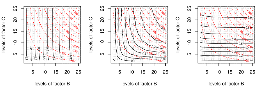
Figure 1: Power and size for the mixed model $(A\succ\boldsymbol{B})\times\boldsymbol{C}$, for $a=6$, $\alpha=0.05$, $\delta=5$, and three variance component assignments $(\sigma_{\beta(\alpha)}^{2},\ \sigma_{\gamma}^{2},\ \sigma_{\alpha\gamma}^{2},\ \sigma_{\beta\gamma(\alpha)}^{2},\ \sigma^{2})$ $=(10,5,0,5,5)$, $(5,5,5,5,5)$, $(0,5,10,5,5)$, from left to right. Each contour plots shows the guaranteed power $P_{\min}=(1-\beta)_{\min}$ (solid curves) overlaid with the size factor $b\cdot c$ (red, dashed hyperbolas) as functions of $b,c\leq 25$, for fixed $n=2$. By Lemma 3.1(ii) the left model is equivalent to $A\succ\boldsymbol{B}\succ\boldsymbol{C}$, such that by Theorem 2.7 the “pivot” parameter is $b$. The middle plot is an approximate $F$-test model (the power is approximated by 10 000 simulations), there is no “pivot” effect. The right model is equivalent to $(A\times\boldsymbol{C})\succ\boldsymbol{B}$, the “pivot” parameter is $c$.

4 Real versus integer parameters

The “pivot” effect for the minimum sample size described in Theorem 2.7(iii) is formulated with the assumption that the parameters are real numbers. The effect also occurs in most practical examples, where the parameters are integers. But we constructed the following example to point out that for integer parameters the “pivot” effect is not a granted fact.

Example 4.1.

Consider the two-way model $A\times\boldsymbol{B}$ with $a=15$, $\alpha=0.1$, $\delta=7$, $(\sigma_{\beta(\alpha)}^{2},\sigma^{2})=(0.01,8)$, and required power $P\geq 0.9$. Then for real $b,n\geq 2$, the minimum sample size obtained by Theorem 2.7(iii) occurs for $(b,n)=(4.019937,2)$, where $P=0.9$. For integers $b,n=2,3,\dots$, the minimum sample size occurs for $(b,n)=(3,3)$, where $P=0.902873$. Thus in this example the “pivot” effect is obstructed if we switch from real numbers to integers. In more realistic examples this obstruction does not occur.

Remark 4.2.

While Example 4.1 shows that the transition to integers can obstruct (if by an unrealistic example) the “pivot” effect, we remark that the obstruction is limited, that is, the real number computation has the following valid implication for the integer result. The real number minimum at $(b,n)=(4.019937,2)$, readily computed by using Theorem 2.7(iii), immediately implies that the integer minimum size occurs at $(b,n)$ with $b\cdot n$ between $4.019937\cdot 2$ and $5\cdot 2$, that is,

$$b\cdot n\in\{9,10\},$$

in fact in the example $b\cdot n=9$. A similar implication holds for all models in Table 1.

5 Conclusions

We determine the noncentrality parameter of the exact $F$-test for balanced factorial ANOVA models. From a sharp lower bound for the noncentrality parameter we obtain the power that can be guaranteed in the least favorable case. These results allow us to compute the minimal sample size, but we also provide a structural result for the minimal sample size. The structural result is formulated as a “pivot” effect, which means that one of the factors is more relevant than the others, for the power and thus for the minimum sample size.

ORCID

Bernhard Spangl https://orcid.org/0000-0001-6222-2408
Norbert Kaiblinger https://orcid.org/0000-0001-6280-5929
Peter Ruckdeschel https://orcid.org/0000-0001-7815-4809
Dieter Rasch https://orcid.org/0000-0001-9324-9910

Appendix A Proofs

We include a short proof of the formula for the noncentrality parameter in Lindman (1992, p. 151), formulated here in a more general form.

Lemma A.1.

Let a test statistic $\boldsymbol{F}$ have a noncentral $F$-distribution with numerator and denominator d.f. $df_{1}$ and $df_{2}$, respectively, written as $\boldsymbol{F}=\boldsymbol{Z}_{1}/\boldsymbol{Z}_{2}$, with $q\neq 0$,

$$\begin{aligned} \boldsymbol{Z}_{1}&=q\cdot\boldsymbol{X}_{1}/df_{1},\\ \boldsymbol{Z}_{2}&=q\cdot\boldsymbol{X}_{2}/df_{2},\end{aligned}\qquad\begin{aligned} \boldsymbol{X}_{1}&\sim\chi^{2}(df_{1},\lambda),\\ \boldsymbol{X}_{2}&\sim\chi^{2}(df_{2},0),\end{aligned}$$

and $\boldsymbol{X}_{1},\boldsymbol{X}_{2}$ stochastically independent. Then the noncentrality parameter $\lambda$ satisfies

$$\lambda=\mathit{df_{1}}\cdot\left(\frac{E(\boldsymbol{Z}_{1})}{E(\boldsymbol{Z}_{2})}-1\right).$$

Proof.

Since $E(\boldsymbol{X}_{1})=df_{1}+\lambda$ and $E(\boldsymbol{X}_{2})=df_{2}$, we obtain $E(\boldsymbol{Z}_{1})=q\cdot(1+\lambda/df_{1})$ and $E(\boldsymbol{Z}_{2})=q$. Hence,

$$E(\boldsymbol{Z}_{1})/E(\boldsymbol{Z}_{2})=1+\lambda/df_{1},$$ (A.1)

which implies the expression for $\lambda$ in the lemma. ∎

Remark A.2.

Jensen’s equality implies $E(\boldsymbol{Z}_{1})/E(\boldsymbol{Z}_{2})<E(\boldsymbol{Z}_{1}/\boldsymbol{Z}_{2})=E(\boldsymbol{F})$. For $E(\boldsymbol{F})$, see Johnson, Kotz, and Balakrishnan (1995, formula (30.3a)).

The next lemma summarizes monotonicity properties of the noncentral $F$-distribution from Ghosh (1973), listed in Hocking (2003, Sec. 16.4.2), see also Finner and Roters (1997, Theorem 4.3) with a sharper statement. Recall that for $0\leq\gamma\leq 1$, we let $F_{\mathit{df_{1}},\mathit{df_{2}};\gamma}$ denote the $\gamma$-quantile of the central $F$-distribution with $\mathit{df_{1}}$ and $\mathit{df_{2}}$ degrees of freedom.

Lemma A.3.

Let $F$ be distributed according to the noncentral $F$-distribution $F_{\mathit{df_{1}},\mathit{df_{2}}}^{\lambda}$ with noncentrality parameter $\lambda$. Then referring to the probability $\mathbb{P}(F>F_{\mathit{df_{1}},\mathit{df_{2}};\gamma})$ as power, we have if $\mathit{df_{1}}$ decreases and $\mathit{df_{2}}$, $\lambda$ increase, then the power increases. That is, we have the implication

$$\left.\begin{aligned} \mathit{df_{1}}&\geq\mathit{df_{1}^{\prime}}\\ \mathit{df_{2}}&\leq\mathit{df_{2}^{\prime}}\\ \lambda&\leq\lambda^{\prime}\end{aligned}\quad\right\}\qquad\Rightarrow\qquad\mathbb{P}(F>F_{\mathit{df_{1}},\mathit{df_{2}};\gamma})\leq\mathbb{P}(F^{\prime}>F_{\mathit{df_{1}^{\prime}},\mathit{df_{2}^{\prime}};\gamma})$$

with $F\sim F_{\mathit{df_{1}},\mathit{df_{2}}}^{\lambda}$ and $F^{\prime}\sim F_{\mathit{df_{1}^{\prime}},\mathit{df_{2}^{\prime}}}^{\lambda^{\prime}}$ .

Proof.

For varying $\mathit{df_{1}}$, see Ghosh (1973, Thm. 6). For varying $\mathit{df_{2}}$, apply Ghosh (1973, Thm. 5) with $\lambda_{0}=0$. For varying $\lambda$, see Witting (1985, p. 219, Satz 2.36(b)) or Bhattacharya and Burman (2016, p. 53, Exercise 2.9). ∎

Proof of Theorem 2.1.

We prove the result only for the model $A\succ\boldsymbol{B}\succ\boldsymbol{C}$, the proofs for the other models are analogous. In the expected mean squares table (Rasch, Pilz, Verdooren, and Gebhardt, 2011, p. 100, Table 3.15) the two expressions

$$E(\boldsymbol{M\!S}_{A}) =\sigma^{2}+n\sigma_{\gamma(\alpha\beta)}^{2}+cn\sigma_{\beta(\alpha)}^{2}+\frac{bcn}{a-1}\sum_{i}\alpha_{i}^{2}$$ (A.2)

$$E(\boldsymbol{M\!S}_{B\,\text{in}\,A}) =\sigma^{2}+n\sigma_{\gamma(\alpha\beta)}^{2}+cn\sigma_{\beta(\alpha)}^{2}$$

are equal under the null hypothesis $H_{0}$ of no $A$-effects. Hence, $H_{0}$ can be tested by the exact $F$-test

$$\boldsymbol{F}_{A}=\frac{\boldsymbol{M\!S}_{A}}{\boldsymbol{M\!S}_{B\,\text{in}\,A}}~{},$$ (A.3)

which under $H_{0}$ is central $F$-distributed, in general noncentral $F$-distributed. From the ANOVA table (Rasch, Pilz, Verdooren, and Gebhardt, 2011, p. 91, Table 3.10) the numerator and denominator d.f. are $\mathit{df_{1}}=a-1$ and $\mathit{df_{2}}=a(b-1)$, respectively. By Lemma A.1 the noncentrality parameter $\lambda$ is thus

$$\lambda =\frac{bcn\sum_{i}\alpha_{i}^{2}}{\sigma^{2}+n\sigma_{\gamma(\alpha\beta)}^{2}+cn\sigma_{\beta(\alpha)}^{2}}=b\cdot\frac{\sum_{i}\alpha_{i}^{2}}{\sigma_{\beta(\alpha)}^{2}+\frac{1}{c}\sigma_{\gamma(\alpha\beta)}^{2}+\frac{1}{cn}\sigma^{2}}~{}.$$ (A.4)

∎

Remark A.4.

1. The formula (A.4) allows us to point out the difference of our results compared to the previous literature (Rasch, Pilz, Verdooren, and Gebhardt, 2011, p.58–59). In fact, the expression $bcn$ in the numerator at the left-hand side of (A.4) coincides with the expression $C$ in Rasch, Pilz, Verdooren, and Gebhardt (2011, Table 3.2), but note that the denominator is distinct. The exact expression for $\lambda$ in (A.4) has the sum of variance components $\sigma_{y}^{2}=\sigma^{2}+\sigma_{\gamma(\alpha\beta)}^{2}+\sigma_{\beta(\alpha)}^{2}$ replaced by the linear combination $\sigma^{2}+n\sigma_{\gamma(\alpha\beta)}^{2}+cn\sigma_{\beta(\alpha)}^{2}$, see also Rasch and Verdooren (2020). The fourth author and Rob Verdooren have acknowledged our results and update their available R-programs accordingly, note in Rasch and Verdooren (2020) some citation numbers have been mixed up. To reproduce the examples of the present paper, R-code is available from the first author.

2. The transformation from the left-hand side to the right-hand side in (A.4) shifts the attention from the product of parameters $bcn$ to the single parameter $b$. This observation is the key to our general “pivot” effect result (Theorem 2.7).

3. To verify the details of Table 1 note that the expected mean squares table entries used in the proof of Theorem 2.1 depend on the factors being fixed or random.

Proof of Theorem 2.4.

1. As above we prove the result for the model $A\succ\boldsymbol{B}\succ\boldsymbol{C}$. Since

   $$\sigma_{\beta(\alpha)}^{2}+\frac{1}{c}\sigma_{\gamma(\alpha\beta)}^{2}+\frac{1}{cn}\sigma^{2}\leq\underbrace{\sigma_{\beta(\alpha)}^{2}+\sigma_{\gamma(\alpha\beta)}^{2}+\sigma^{2}}_{\displaystyle\sigma_{y,\mathit{active}}^{2}},$$ (A.5)

   we obtain

   $$\lambda=b\cdot\frac{\sum_{i}\alpha_{i}^{2}}{\sigma_{\beta(\alpha)}^{2}+\frac{1}{c}\sigma_{\gamma(\alpha\beta)}^{2}+\frac{1}{cn}\sigma^{2}}\geq b\cdot\frac{\sum_{i}\alpha_{i}^{2}}{\sigma_{y,\mathit{active}}^{2}},$$ (A.6)

   and the Szőkefalvi-Nagy inequality (Alpargu and Styan, 2000, p. 11; Brauer and Mewborn, 1959; Gutman, Das, Furtula, Milovanović, and Milovanović, 2017; Kaiblinger and Spangl, 2020; Sharma, Gupta, and Kapoor, 2010; Szőkefalvi-Nagy, 1918) states that

   $$\sum_{i}\alpha_{i}^{2}\geq\frac{(\alpha_{\max}-\alpha_{\min})^{2}}{2}=\frac{\delta^{2}}{2}~{}.$$ (A.7)

2. By Kaiblinger and Spangl (2020) we have for the $(v\times a)$ matrix $(\alpha_{i(j)})_{i,j}$ and for the $(u\times v\times a)$ array $(\alpha_{i(jk)})_{i,j,k}$,

   $$\sum_{i,j}\alpha_{i(j)}^{2}\geq\frac{\delta^{2}}{2}\cdot\frac{m}{m-1}\quad\text{ and }\quad\sum_{i,j,k}\alpha_{i(jk)}^{2}\geq\frac{\delta^{2}}{2}\cdot\frac{m_{2}m_{3}}{(m_{2}-1)(m_{3}-1)},$$ (A.8)

   respectively. ∎

Proof of Theorem 2.7.

1. We consider the parameters as competitors in

   not increasing $$\mathit{df_{1}} \mathit{df_{2}} \lambda$$   and   increasing and . (A.9)

   For each model in Table 1, we analyze the effect of the parameters on $\mathit{df_{1}}$, $\mathit{df_{2}}$ and $\lambda$, using the arguments illustrated in Example A.5 below. The inspection yields that for each model there is a sole winner, which we call the “pivot” parameter. We exemplify the scoring for four models:

   	$A\succ B\succ C$	$A\succ\boldsymbol{B}\succ\boldsymbol{C}$	$V\succ A\succ B$	$V\succ A\succ\boldsymbol{B}$
   parameters	$b,c,n$	$b,c,n$	$v,b,n$	$v,b,n$
   least increase in $\mathit{df_{1}}$	$b,c,n$	$b,c,n$	$b,n$	$b,n$
   most increase in $\mathit{df_{2}}$	$n$	$b$	$n$	$b$
   most increase in $\lambda$	$b,c,n$	$b$	$b,n$	$b$
   $\Rightarrow$ pivot	$n$	$b$	$n$	$b$

   Since by Lemma A.3 the lead in (A.9) also means the lead in power increase, we thus obtain that the “pivot” yields the maximal power increase.

2. Start with minimal parameters and apply (i).

3. is equivalent to (ii). ∎

Example A.5.

We illustrate the proof of Theorem 2.7(i) by showing the typical argument for most increase in $\mathit{df_{2}}$ and the typical argument for most increase in $\lambda$.

1. In the model $A\succ B\succ C$ the parameter $n$ is more effective than $b$ or $c$ in increasing $\mathit{df_{2}}$,

   $$\mathit{df_{2}}=abc(n-1)=abcn-abc,$$ (A.10)

   since $b,c,n$ equally increase the positive term of (A.10), but only $n$ does not increase the negative term.

2. For the model $A\succ\boldsymbol{B}\succ\boldsymbol{C}$, the parameter $b$ is more effective than $c$ or $n$ in increasing $\lambda$,

   $$\lambda=\frac{bcn\sum_{i}\alpha_{i}^{2}}{\sigma^{2}+n\sigma_{\gamma(\alpha\beta)}^{2}+cn\sigma_{\beta(\alpha)}^{2}},$$ (A.11)

   since $b,c,n$ equally increase the numerator of (A.11), but only $b$ does not increase the denominator.

References

- Alpargu and Styan (2000, p. 11) Alpargu, G., Styan, G.P.H., 2000. Some comments and a bibliography on the Frucht-Kantorovich and Wielandt inequalities, in: Innovations in Multivariate Statistical Analysis, Springer, 1–38. doi:10.1007/978-1-4615-4603-0
- Behrens (1929) Behrens, W.V., 1929. Ein Beitrag zur Fehlerberechnung bei wenigen Beobachtungen. Landw. Jahrb., 68, 807–837. (German).
- Bhattacharya and Burman (2016) Bhattacharya, P.K., Burman, P., 2016. Theory and Methods of Statistics. Elsevier. ISBN 9780128041239
- Brauer and Mewborn (1959) Brauer, A., Mewborn, A.C., 1959. The greatest distance between two characteristic roots of a matrix. Duke Math. J. 26 (4), 653–661. doi:10.1215/S0012-7094-59-02663-8
- Canavos and Koutrouvelis (2009) Canavos, G., Koutrouvelis, I., 2009. An Introduction to the Design & Analysis of Experiments. Pearson. ISBN 978-0136158639
- Davenport and Webster (1972) Davenport, J.M., Webster, J.T., 1972. Type-I Error and Power of a Test Involving a Satterthwaite’s Approximate F-Statistic. Technometrics 14 (3), 555–569.
- Davenport and Webster (1973) Davenport, J.M., Webster, J.T., 1973. A Comparison of Some Approximate F-Tests. Technometrics 15 (4), 779–789.
- Doncaster and Davey (2007) Doncaster, C.P., Davey, A.J.H., 2007. Analysis of Variance and Covariance: How to Choose and Construct Models for the Life Sciences. Cambridge Univ. Press. doi:10.1017/CBO9780511611377
- Finner and Roters (1997) Finner, H., Roters, M., 1997. Log-concavity and inequalities for chi-square, F and beta distributions with applications in multiple comparisons. Stat. Sinica 7 (3), 771–787.
- Fox (2015) Fox, J., 2015. Applied Regression Analysis and Generalized Linear Models. (3rd ed.) SAGE Publ. ISBN 9781452205663
- Ghosh (1973) Ghosh, B.K., 1973. Some monotonicity theorems for , and distributions with applications. J. R. Stat. Soc., Ser. B 35 (3), 480–492.
- Gutman, Das, Furtula, Milovanović, and Milovanović (2017) Gutman, I., Das, K.C., Furtula, B., Milovanović, E., Milovanović, I., 2017. Generalizations of Szőkefalvi Nagy and Chebyshev inequalities with applications in spectral graph theory. Appl. Math. Comput. 313, 235–244. doi:10.1016/j.amc.2017.05.064
- Hocking (2003) Hocking, R.R., 2003. Methods and Applications of Linear Models: Regression and the Analysis of Variance. Wiley. doi:10.1002/0471434159
- Hudson and Krutchkoff (1968) Hudson, J.D. Jr, Krutchkoff, R.G., 1968. A Monte Carlo investigation of the size and power of tests employing Satterthwaite’s synthetic mean squares. Biometrika 55 (2), 431–433.
- Jiang (2007) Jiang, J., 2007. Linear and Generalized Linear Mixed Models and Their Applications. Springer. doi:10.1007/978-0-387-47946-0
- Johnson, Kotz, and Balakrishnan (1995) Johnson, N.L., Kotz, S., Balakrishnan, N., 1995. Continuous Univariate Distributions, Volume 2. (2nd ed.) ISBN 9780471584940
- Kaiblinger and Spangl (2020) Kaiblinger, N., Spangl, B., 2020. An inequality for the analysis of variance. Math. Inequal. Appl. 23 (3), 961–969. doi:10.7153/mia-2020-23-74
- Lindman (1992) Lindman, H.R., 1992. Analysis of Variance in Experimental Design. Springer. doi:10.1007/978-1-4613-9722-9
- Lorenzen and Anderson (2019) Lorenzen, T., Anderson, V., 2019. Design of Experiments: A No-Name Approach. CRC Press. ISBN 9780367402327
- Maxwell, Delaney, and Kelley (2017) Maxwell, S.E., Delaney, H.D., Kelley, K., 2017. Designing Experiments and Analyzing Data. Routledge. ISBN 9781138892286
- Montgomery (2017) Montgomery, D., 2017. Design and Analysis of Experiments. Wiley. ISBN 978-1-119-32093-7
- Myers (2010) Myers, J.L., Well, A.D., 2010. Research Design and Statistical Analysis. Taylor & Francis. doi:10.4324/9780203726631
- Rasch (1971) Rasch, D., 1971. Gemischte Klassifikation der dreifachen Varianzanalyse. Biometr. Z. 13 (1), 1–20. (German). doi:10.1002/bimj.19710130102
- Rasch, Pilz, Verdooren, and Gebhardt (2011) Rasch, D., Pilz, J., Verdooren, R., Gebhardt, A., 2011. Optimal Experimental Design with R. Chapman & Hall. doi:10.1007/s00362-012-0473-y
- Rasch and Schott (2018) Rasch, D., Schott, D., 2018. Mathematical Statistics. Wiley. doi:10.1002/9781119385295
- Rasch, Spangl, and Wang (2012) Rasch, D., Spangl, B., Wang, M., 2012. Minimal experimental size in the three way ANOVA cross classification model with approximate -tests. Commun. Stat., Simulation Comput. 41 (7), 1120–1130. doi:10.1080/03610918.2012.625832
- Rasch and Verdooren (2020) Rasch, D., Verdooren, R., 2020. Determination of minimum and maximum experimental size in one-, two- and three-way ANOVA with fixed and mixed models by R. J. Stat. Theory Pract. 14 (4), #57. doi:10.1007/s42519-020-00088-6
- Rasch, Verdooren, and Pilz (2020) Rasch, D., Verdooren, R., Pilz, J., 2020. Applied Statistics. Wiley. doi:10.1002/9781119551584
- Sahai and Ageel (2000) Sahai, H., Ageel, M.I., 2000. The Analysis of Variance, Birkhäuser. doi:10.1007/978-1-4612-1344-4
- Satterthwaite (1946) Satterthwaite, F., 1946. An approximate distribution of estimates of the variance components. Biometrics Bull. 2 (6), 110–114. doi:10.2307/3002019
- Scheffé (1959) Scheffé, H., 1959. The Analysis of Variance. Wiley. ISBN 9780471345053
- Searle and Gruber (2017) Searle, S.R., Gruber, M.H.J., 2017. Linear Models. (2nd ed.) Wiley. ISBN 9781118952856
- Sharma, Gupta, and Kapoor (2010) Sharma, R., Gupta, M., Kapoor, G., Some better bounds on the variance with applications. J. Math. Inequal. 4(3), 355–363. doi:10.7153/jmi-04-32
- Szőkefalvi-Nagy (1918) Szőkefalvi-Nagy, J., 1918. Über algebraische Gleichungen mit lauter reellen Wurzeln. Jahresber. Dtsch. Math.-Ver. 27, 37–43. (German).
- Wang, Rasch, and Verdooren (2005) Wang, M., Rasch, D., Verdooren, R., 2005. Determination of the size of a balanced experiment in mixed ANOVA models using the modified approximate F-test. J. Stat. Plann. Inference 132, 183–201. doi:10.1016/j.jspi.2004.06.022
- Welch (1938) Welch, B.L., The significance of the difference between two means when the population variances are unequal. 1938. Biometrika 29 (3-4), 350–362. doi:10.1093/biomet/29.3-4.350
- Welch (1947) Welch, B.L., 1947. The generalization of ‘Student’s’ problem when several different population variances are involved. Biometrika 34 (1-2), 28–35. doi:10.1093/biomet/34.1-2.28
- Witting (1985) Witting, H., 1985. Mathematische Statistik I. Springer. (German). doi:10.1007/978-3-322-90150-7