Magnetic degeneracy points in interacting two-spin systems:
geometrical patterns, topological charge distributions, and their stability

Abstract

Spectral degeneracies of quantum magnets are often described as diabolical points or magnetic Weyl points, which carry topological charge. Here, we study a simple, yet experimentally relevant quantum magnet: two localized interacting electrons subject to spin-orbit coupling. In this setting, the degeneracies are not necessarily isolated points, but can also form a line or a surface. We identify ten different possible geometrical patterns formed by these degeneracy points, and study their stability under small perturbations of the Hamiltonian. Stable structures are found to depend on the relative sign of the determinants of the two $g$-tensors, $\cal S$. Both for ${\cal S}=+1$ and ${\cal S}=-1$, two stable configurations are found, and three out of these four configurations are formed by pairs of Weyl points. These stable regions are separated by a surface of almost stable configurations, with a structure akin to co-dimension one bifurcations.

I Introduction.

Nuclear and electron spins are ubiquitous constituents in condensed matter physics. Already a few interacting quantum spins exhibit a rich variety of phenomena in rather different settings such as molecular magnets Wernsdorfer and Sessoli (1999); Garg (2010); Bruno (2006), magnetic adatoms Wiesendanger (2009); Spinelli et al. (2015), or spin-based quantum bits Hanson et al. (2007); Zwanenburg et al. (2013), to name a few. When studied in the three-dimensional parameter space defined by an external magnetic field, all these quantum magnets possess an intrinsic geometrical and topological structure, characterized by concepts Berry (1984); Wilczek and Shapere (1989) such as the Berry phase, the Berry curvature, and the Chern number. This geometrical structure plays an important role in coherent dynamics San-Jose et al. (2008) as well as in decoherence effects San-Jose et al. (2006), providing a strong motivation for exploration.

In many cases, topological considerations entail robust phenomena, governed by some global properties, insensitive to microscopic details. The quantized Hall conductance arising in the quantum Hall effect Klitzing et al. (1980); Thouless, D. J. and Kohmoto, M. and Nightingale, M. P. and den Nijs, M. (1982) is a prime example. In this work, we address another robust phenomenonvon Neumann and Wigner ; Herring (1937) rooted in topology, which appears in interacting spin systems subject to a magnetic field, the emergence of ground state degeneracies at certain magnetic fields. In this case, a topological invariant (an appropriately defined global Chern number, to be referred here as the total topological charge) predicts the existence and global properties of ground-state magnetic degeneracy points.Bruno (2006); Gritsev and Polkovnikov (2012); Berry (1984); Garg (2010); Roushan et al. (2014); Scherübl et al. (2019) Most frequently, but not always, these degeneracy points are Weyl pointsScherübl et al. (2019), similar to linearly dispersing band touching points in the band structure of Weyl semimetalsArmitage et al. (2018), and also appearing in various physical contextsRiwar et al. (2016); Stenger and Pekker (2019); Gao et al. (2016). The precise relation of the total topological charge, the magnetic degeneracy points, and the topological charge of these points is explained in the context of molecular magnets and spin-orbit-coupled double quantum dots in Refs. Bruno, 2006 and Scherübl et al., 2019, respectively.

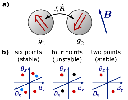
Figure 1: Magnetic degeneracy points of two interacting spin-1/2 electrons. (a) Exchange interaction between the spins is described by its strength $J$ and a rotation $\hat{\text{\boldmath{$R$}}}$. External magnetic field $B$ couples to the spins through the $g$-tensors. (b) Geometry and topological charge distribution of magnetic degeneracy points for $\text{det}\,\hat{\text{\boldmath{$g$}}}_{\text{L}},\text{det}\,\hat{\text{\boldmath{$g$}}}_{\text{R}}>0$. Colors indicate topological charge: $+1$ (red), $-1$ (blue), $0$ (black). Six-point and two-point patterns are stable, and the generic transition between these patterns is when two oppositely charged pairs meet and their charges annihilate each other (four points).

Even though a nonzero total topological charge guarantees the existence of magnetic degeneracy points, its value does not provide a definite answer to the following questions. (i) What is the geometrical pattern (isolated points, lines, surfaces, or their combinations) drawn by the magnetic degeneracy points in the three-dimensional magnetic parameter space? (ii) How is the topological charge carried by the magnetic degeneracy points distributed among the points? (iii) Are different geometrical patterns and topological charge distributions stable against small perturbations of the system’s Hamiltonian? These are nontrivial questions, and answering them probably requires extensive numerical investigations, in general.

Here, we address questions (i), (ii), and (iii) for a specific, experimentally relevant setup, a spin-orbit-coupled interacting two-spin systemKavokin (2004); Nowack et al. (2007); Nadj-Perge et al. (2010, 2012); Schroer et al. (2011); Harvey-Collard et al. (2019); Tanttu et al. (2019); Scherübl et al. (2019), and obtain exact results. We provide a full classification of geometrical patterns (and corresponding topological charge density patterns) of the ground-state magnetic degeneracy points of this setup; this ‘zoo’ of patterns is introduced in Tables 1 and 2. Finding the degeneracy points is reduced to the eigenvalue problem of a $3\times 3$ non-symmetric real matrix, and hence our analysis inherits key features of different physics subdisciplines, such as bifurcation theoryGuckenheimer and Holmes (1983) and non-Hermitian wave mechanicsBerry (2004); Heiss (2012), where similar eigenvalue problems play important roles. Beyond fundamental interest, the properties of magnetic degeneracy points are in fact practically important for control and readout of spin-based quantum bits; two-electron singlet-triplet degeneracy points, e.g., are often exploited for spin initialization, control and readoutPetta et al. (2005); Hanson et al. (2007); Reilly et al. (2008); Petta et al. (2010); Harvey-Collard et al. (2019); Tanttu et al. (2019).

We consider a system of two interacting localized electrons, subject to spin-orbit interaction, and assume that they are placed in a homogeneous magnetic (Zeeman) field (Fig. 1a). This system can be described by a $4\times 4$ Hamiltonian matrixScherübl et al. (2019)

$$H = H_{\text{Z}}+H_{\text{int}},$$ (1)

$$H_{\text{Z}} = \mu_{\text{B}}\text{\boldmath{$B$}}\left(\hat{\text{\boldmath{$g$}}}_{\text{L}}\text{\boldmath{$S$}}_{\text{L}}+\hat{\text{\boldmath{$g$}}}_{\text{R}}\text{\boldmath{$S$}}_{\text{R}}\right),$$ (2)

$$H_{\text{int}} = J\text{\boldmath{$S$}}_{\text{L}}\hat{\text{\boldmath{$R$}}}\text{\boldmath{$S$}}_{\text{R}}.$$ (3)

Here, $H_{\text{Z}}$ is the Zeeman interaction with the external homogeneous magnetic field $B$, $H_{\text{int}}$ is the spin-orbit-affected exchange interaction between the two electrons, $\mu_{\text{B}}$ is the Bohr-magneton, $\hat{\text{\boldmath{$g$}}}_{\text{L}}$ and $\hat{\text{\boldmath{$g$}}}_{\text{R}}$ are the real-valued, spin-orbit-affected $g$-tensors of the two electrons, $\text{\boldmath{$S$}}_{\text{L}}$ and $\text{\boldmath{$S$}}_{\text{R}}$ are the spin vector operators represented by $1/2$ times the spin-1/2 Pauli matrices, $J>0$ is the strength of the exchange interaction, and $\hat{\text{\boldmath{$R$}}}$ is a real, $3\times 3$ special orthogonal matrix accounting for the spin-orbit interaction in the exchange term. The exchange term $H_{\text{int}}$ was derived from a two-site Hubbard model using quasidegenerate perturbation theory in Supplementary Note 2 of Ref. Scherübl et al., 2019, see Eqs. (S2) and (S3) therein, which imply that this term is a positive prefactor times a rotation.

The $g$-tensors are arbitrary real matrices, which are not necessarily symmetric. For concreteness, let us first focus on the case when the determinants of both $g$-tensors are positive, $\text{det}(\hat{\text{\boldmath{$g$}}}_{\text{L}}),\,\text{det}(\hat{\text{\boldmath{$g$}}}_{\text{R}})>0$. The elements of the three $3\times 3$ matrices $\hat{\text{\boldmath{$g$}}}_{L}$, $\hat{\text{\boldmath{$g$}}}_{R}$, and $\hat{\text{\boldmath{$R$}}}$ are determined by microscopic details (spin-orbit interaction, confinement potential, etc.), but here we treat them as possibly independent phenomenological parameters.

In our topological considerations, we distinguish the three Cartesian magnetic-field components $B_{x}$, $B_{y}$, $B_{z}$ in the Hamiltonian as ‘primary’ parameters, and refer to further parameters as ‘secondary’ ones. In this nomenclature, secondary parameters are fixed, while primary parameters are thought of as external parameters, varied continuously. At certain points within the space of primary parameters, the ground state of $H$ becomes degenerate. We refer to these points as magnetic degeneracy points.

We have studied this two-spin system in detail in our recent work Scherübl et al. (2019). There we have shown that in the case $\text{det}(\hat{\text{\boldmath{$g$}}}_{\text{L}}),\,\text{det}(\hat{\text{\boldmath{$g$}}}_{\text{R}})>0$, (i) topological considerations guarantee the existence of ground-state magnetic degeneracy points (often, but not always, magnetic Weyl points), irrespective of microscopic details of the Hamiltonian, (ii) the degeneracy points carry topological charge, and the total topological charge carried by all degeneracy points of the three-dimensional magnetic-field parameter space sums up to +2. By numerical work and intuitive considerations, we have demonstrated four different geometrical patterns formed by the magnetic degeneracy points, and the corresponding topological charge distributions: (A) A sphere, carrying a surface topological charge of +2. This is the case without spin-orbit interaction, when the $g$-tensors are isotropic and the exchange interaction is of antiferromagnetic Heisenberg type ($J\text{\boldmath{$S$}}_{\text{L}}\cdot\text{\boldmath{$S$}}_{\text{R}}$). This case also provides an example where the magnetic degeneracy points are not Weyl points. (B) Two isolated (Weyl) points, each carrying charge +1. (C) Six isolated (Weyl) points, four of them carrying charge +1, two of them carrying charge -1. (D) Four isolated points, two of them carrying charge +1, the other two carrying no charge. (See Fig. 1b of this work or Fig. 4a of Ref. Scherübl et al., 2019.)

We note that we use the term Weyl point to label an isolated degeneracy point that possesses all of the following properties: (1) the energy splitting in its vicinity is linearly increases with small deviation in the parameter space, in all directions, (2) the degeneracy is twofold, and (3) the absolute value of its topological charge is one. Accordingly, we did not label the charge-neutral degeneracy points in case (D) above as Weyl-points, since they violate both (1) and (3). In the condensed-matter literature, band degeneracy points not showing at least one of the above three properties are sometimes called multi-Weyl pointsFang et al. (2012); Yan and Wang (2017); Ahn et al. (2017); Huang et al. (2017); we do not use this terminology here.

Going beyond our earlier numerical study, here we develop an analytical approach, which allows for a complete classification of the geometrical and topological structure of magnetic degeneracy points. For this analysis, it is important to distinguish three cases defined by the three possible values of the total topological charge $\cal Q$. This charge is the sum of the $g$-tensor determinants, i.e., ${\cal Q}=\text{sgn(det}\ \hat{\text{\boldmath{$g$}}}_{\text{L}})+\text{sgn(det}\ \hat{\text{\boldmath{$g$}}}_{\text{R}})$, and hence ${\cal Q}\in\{-2,0,2\}$ We will show that the geometrical patterns are the same in case ${\cal Q}=+2$ (Table 1) and case ${\cal Q}=-2$, although the topological charges are the opposite in the two cases. Also, we will show that the geometrical patterns are distinct in the case ${\cal Q}=0$ (Table 2). Rephrasing this in terms of the relative sign ${\cal S}=\text{sgn}[\text{det}(\hat{\text{\boldmath{$g$}}}_{\text{L}})\cdot\text{det}(\hat{\text{\boldmath{$g$}}}_{\text{R}})]$, we can say that the geometrical patterns are different for the two possible values ${\cal S}\in\{-1,+1\}$.

For ${\cal S}=+1$ we obtain a sixfold classification of geometrical patterns of magnetic degeneracy points (Table 1), corresponding to six different topological charge distributions (i.e., two more beyond the ones identified in Ref. Scherübl et al., 2019), and further four possible classes are identified for ${\cal S}=-1$. These form altogether ten geometrical classes.

Furthermore, we use our approach to characterize the stability of these patterns against small perturbations of the Hamiltonian (see Fig. 1b): we find two stable and one almost stable charge configurations both for ${\cal S}=+1$ and for ${\cal S}=-1$, the almost stable magnetic configuration forming a generic boundary between stable configurations, similar to bifurcations in the theory of dynamical systems.Guckenheimer and Holmes (1983)

The rest of the paper is structured as follows. In Sec. II, we derive a classification of the geometrical patterns and topological charge density patterns of magnetic degeneracy points for the case ${\cal S}=+1$, with the main results summarized in Table 1. In Sec. III, we analyze the stability of each of these patterns against perturbations of the Hamiltonian. In Sec. IV, we extend the results to case ${\cal S}=-1$, and provide our conclusions in Sec. V.

II Classifications of degeneracy points

II.1 Mapping the degeneracy problem to the eigenproblem of a non-symmetric matrix

Given the Hamiltonian (1), it is not obvious how to analyze the geometrical patterns formed by the magnetic degeneracy points. One could, in principle, find the eigenvalues of the $4\times 4$ Hamiltonian (1) analytically, and investigate, in a very large dimensional parameter space, the conditions under which ground-state degeneracies occur. Numerical diagonalization and numerical search for the magnetic degeneracy points is also an option, but this requires a lot of computational effort and is most likely incomplete Scherübl et al. (2019).

Fortunately, for the specific Hamiltonian, Eq. (1), a simple observation allows for a fully analytical treatment of the problem. As a first step, we introduce a local spin transformation that leaves the left spin invariant, $\text{\boldmath{$S$}}^{\prime}_{\text{L}}=\text{\boldmath{$S$}}_{\text{L}}$, but it rotates the right spin with the rotation appearing in the exchange term, $\text{\boldmath{$S$}}^{\prime}_{R}=\hat{\text{\boldmath{$R$}}}\text{\boldmath{$S$}}_{R}$. This transformation renders the exchange interaction isotropic. The transformed Hamiltonian now reads

$$H^{\prime}=\mu_{\text{B}}\left(\text{\boldmath{$B$}}_{\text{L,eff}}\text{\boldmath{$S$}}^{\prime}_{\text{L}}+\text{\boldmath{$B$}}_{\text{R,eff}}\text{\boldmath{$S$}}^{\prime}_{\text{R}}\right)+J\text{\boldmath{$S$}}^{\prime}_{\text{L}}\text{\boldmath{$S$}}^{\prime}_{\text{R}},$$ (4)

where the effective magnetic fields felt by the left and right spins read $\text{\boldmath{$B$}}_{\text{L,eff}}=\text{\boldmath{$B$}}\hat{\text{\boldmath{$g$}}}_{\text{L}}$ and $\text{\boldmath{$B$}}_{\text{R,eff}}=\text{\boldmath{$B$}}\hat{\text{\boldmath{$g$}}}_{\text{R}}\hat{\text{\boldmath{$R$}}}^{-1}$. Clearly, if these effective magnetic fields are parallel, then we can take the spin quantization axis $z$ along the direction of the effective magnetic fields. This choice implies that $S^{\prime}_{\text{L}z}+S^{\prime}_{\text{R}z}$ is conserved, and therefore, if the effective fields point in the same direction, then there must be a ground-state level crossing as $B$ is increased from zero to infinity along this direction (Appendix C).

These observations imply that for finding the magnetic degeneracy points, we do not have to solve the eigenvalue problem of the $4\times 4$ Hamiltonian, but it is instead sufficient to find the magnetic-field directions for which $\text{\boldmath{$B$}}_{\text{L,eff}}\parallel\text{\boldmath{$B$}}_{\text{R,eff}}$. An elementary proof shows that this condition is satisfied, if and only if $B$ is a (left) eigenvector of the $3\times 3$ matrix

$$\hat{\text{\boldmath{$M$}}}=\hat{\text{\boldmath{$g$}}}_{\text{L}}\hat{\text{\boldmath{$R$}}}\hat{\text{\boldmath{$g$}}}_{\text{R}}^{-1}.$$ (5)

A magnetic degeneracy point is found in this direction if the eigenvector belongs to a positive eigenvalue of $\hat{\text{\boldmath{$M$}}}$. Note that $\hat{\text{\boldmath{$M$}}}$ is real, but in general it is not symmetric.

Eigenpattern label	Multiplicities of eigenvalues	Geometric pattern	Topological charge distribution	Degeneracy points	Jordan normal form	Stability codimension
(I)	(1/1,1/1,1/1)	six points	$4\times(+1)$, $2\times(-1)$		$\begin{pmatrix}a&0&0\\ 0&b&0\\ 0&0&c\\ \end{pmatrix}$	0 (stable)
(II)	(2/2,1/1)	two points, loop	$2\times(+1)$, $0$		$\begin{pmatrix}a&0&0\\ 0&a&0\\ 0&0&b\\ \end{pmatrix}$	3
(III)	(2/1,1/1)	four points	$2\times(+1)$, $2\times 0$		$\begin{pmatrix}a&1&0\\ 0&a&0\\ 0&0&b\\ \end{pmatrix}$	1 (almost stable)
(IV)	(3/3)	closed surface	$2$ (surface charge)		$\begin{pmatrix}a&0&0\\ 0&a&0\\ 0&0&a\\ \end{pmatrix}$	8
(V)	(3/2)	loop	$2$ (line charge)		$\begin{pmatrix}a&1&0\\ 0&a&0\\ 0&0&a\\ \end{pmatrix}$	4
(VI)	(3/1)	two points	$2\times(+1)$		$\begin{pmatrix}a&1&0\\ 0&a&1\\ 0&0&a\\ \end{pmatrix}$	2
(VII)	(1/1)	two points	$2\times(+1)$		$\begin{pmatrix}a&0&0\\ 0&\text{n/c}&0/1\\ 0&0&\text{n/c}\\ \end{pmatrix}$	0 (stable)

Table 1: Zoo of geometrical patterns and topological charge density patterns of magnetic ground-state degeneracies of a spin-orbit-coupled two-spin system. Classification is based on the eigenpatterns of the $3\times 3$ real matrix $\hat{\text{\boldmath{$M$}}}$ with positive determinant, see text. In the second column, we display the algebraic and geometrical multiplicities of positive eigenvalues. Each eigenpattern implies a geometrical pattern of the magnetic degeneracy points, which in turn implies a topological charge density pattern. The fifth column schematically shows the geometrical pattern of degeneracy points, and the topological charge of each geometrical element: $+2$ (orange), $+1$ (red), $0$ (magenta), $-1$ (blue). In sixth row, the Jordan normal form may have negative or complex eigenvalues (‘n/c’), and if there is only a single negative eigenvalue, then the superdiagonal element of its Jordan block can be either 0 or 1. The last column shows the stability codimension of the eigenpatterns, i.e., the number of linearly independent constraints for a small perturbation not to break the pattern.

II.2 Eigenpattern of the matrix $\hat{\text{\boldmath{$M$}}}$ and the geometrical pattern of the magnetic degeneracy points

As we now show, the structure of the eigenvalues and eigenvectors of the matrix $\hat{\text{\boldmath{$M$}}}$ implies the geometrical pattern of the magnetic degeneracy points. For concreteness, throughout the rest of Sec. II and also in Sec. III, we focus on the case where the determinants of both $g$-tensors are positive, $\text{det}(\hat{\text{\boldmath{$g$}}}_{\text{L}}),\,\text{det}(\hat{\text{\boldmath{$g$}}}_{\text{R}})>0$, that is, ${\cal S}=+1$ and ${\cal Q}=+2$. The results obtained trivially carry over to the case $\det(\hat{\text{\boldmath{$g$}}}_{\text{L}}),\det(\hat{\text{\boldmath{$g$}}}_{\text{R}})<0$ (${\cal S}=+1$, ${\cal Q}=-2$), with the only modification that the total topological charge of the ground-state magnetic degeneracy points has opposite sign in the latter case, and correspondingly, all topological charges in the discussions below are reversed.

The case ${\cal S}=-1$ (${\cal Q}=0$) is, however, quite different. Then the total topological charge of the magnetic degeneracy points adds up to zero, implying a completely different structure of the eigenproblem of $\hat{\text{\boldmath{$M$}}}$, and thereby different geometrical patterns and topological charge distributions. This case will be discussed in Sec. IV.

For $\text{det}(\hat{\text{\boldmath{$g$}}}_{\text{L}}),\,\text{det}(\hat{\text{\boldmath{$g$}}}_{\text{R}})>0$, the $3\times 3$ matrix $\hat{\text{\boldmath{$M$}}}$ is real but non-symmetric in general, and it has a positive determinant, because the $g$-tensors have positive determinants, and $\text{det}\,\hat{\text{\boldmath{$R$}}}=1$. To see the possible geometries of the magnetic degeneracy points, we first have to identify qualitatively different solutions of the eigenproblem of $\hat{\text{\boldmath{$M$}}}$.

As we show below, for $\text{det}(\hat{\text{\boldmath{$g$}}}_{\text{L}}),\,\text{det}(\hat{\text{\boldmath{$g$}}}_{\text{R}})>0$ there are 7 different cases, labelled from (I) to (VII) in Table 1, that are classified by the number of positive eigenvalues, and their algebraic and geometric multiplicities. (For a brief summary of the relevant concepts and relations of linear algebra, see Appendix A.) We call these cases the eigenpatterns of the matrix $\hat{\text{\boldmath{$M$}}}$, and will use, e.g., $\text{ep}(\hat{\text{\boldmath{$M$}}})=\text{(IV)}$, to denote that the eigenpattern of $\hat{\text{\boldmath{$M$}}}$ is (IV).

For $\text{ep}(\hat{\text{\boldmath{$M$}}})=\text{(I)}$, the matrix $\hat{\text{\boldmath{$M$}}}$ has three different positive eigenvalues, $a$, $b$ and $c$. The algebraic and geometric multiplicities are all 1, as denoted in the second column of Table 1. Let us denote the normalized left eigenvectors with $\text{\boldmath{$v$}}_{a}$, $\text{\boldmath{$v$}}_{b}$ and $\text{\boldmath{$v$}}_{c}$. Then, there are six magnetic degeneracy points, one time-reversed pair associated to each eigenvector $\text{\boldmath{$v$}}_{\alpha}$, appearing if the magnetic field is aligned or antialigned with those eigenvectors. The locations of the degeneracy points in the original magnetic-field parameter space are

$$\text{\boldmath{$B$}}_{\alpha,\pm}=\pm B_{\alpha}\cdot\text{\boldmath{$v$}}_{\alpha},\,\,\,(\alpha\in a,b,c).$$ (6)

The expressions for the critical fields $B_{\alpha}$, and their derivations are summarized in Appendix C. Topological charges of these degeneracy points are discussed below.

Different eigenpatterns arise when $\hat{\text{\boldmath{$M$}}}$ has two different positive eigenvalues, $a$ and $b$, see Table 1, rows (II) and (III). In these cases, one of these eigenvalues, say $a$, must have an algebraic multiplicity of 2. (Otherwise, either $\hat{\text{\boldmath{$M$}}}$ would have a third, negative eigenvalue, which is forbidden by the fact the $\hat{\text{\boldmath{$M$}}}$ has positive determinant, or it would have a third, complex eigenvalue, which is forbidden by the fact that complex eigenvalues come in complex-conjugate pairs.) Then, $a$ can have a geometric multiplicity of 2, yielding case (II) in Table 1, or a geometric multiplicity of 1, yielding case (III). In case (II), the magnetic degeneracy points are arranged at two isolated points along the line of $\text{\boldmath{$v$}}_{b}$, at $\text{\boldmath{$B$}}_{b,\pm}=\pm B_{b}\cdot\text{\boldmath{$v$}}_{b}$, and along an ellipse in the plane spanned by the two remaning eigenvectors, $\text{\boldmath{$v$}}_{a_{1}}$ and $\text{\boldmath{$v$}}_{a_{2}}$. See Appendix D for details. In case (III), the magnetic degeneracy points are arranged in four isolated points, similarly at $\text{\boldmath{$B$}}_{a,\pm}=\pm B_{a}\cdot\text{\boldmath{$v$}}_{a}$ and $\text{\boldmath{$B$}}_{b,\pm}=\pm B_{b}\cdot\text{\boldmath{$v$}}_{b}$.

Further eigenpatterns appear when $\hat{\text{\boldmath{$M$}}}$ has a single positive eigenvalue, $a>0$, see rows (IV)-(VII) of Table 1. These eigenvalues can have an algebraic multiplicity of 3, and a geometric multiplicity of 3, yielding case (IV), where the magnetic degeneracy points form a closed surface, an ellipsoid. The simplest example is the case without spin-orbit interaction, where the $g$-tensors and $\hat{\text{\boldmath{$R$}}}$ are all proportional to the unit matrix, and the magnetic degeneracy points form a sphere. Alternatively, $a$ can have an algebraic multiplicity of 3, and a geometric multiplicity of 2, yielding case (V), where the magnetic degeneracy points form a closed loop, an ellipse. Yet another alternative is that $a$ has a geometric multiplicity of 1, yielding case (VI), with two isolated magnetic degeneracy points. Finally, it can also have an algebraic multiplicity of 1, and consequently a geometric multiplicity of 1, denoted as case (VII), yielding two isolated magnetic degeneracy points. This sevenfold classification of the relevant solutions of the eigenvalue problem implies a sixfold classification of the qualitatively different geometrical patterns of the magnetic degeneracy points, since the eigenpatterns (VI) and (VII) yield the same geometry.

II.3 Topological charge-density patterns

We know that the magnetic degeneracy points can also carry a topological charge Scherübl et al. (2019), and for our Hamiltonian with fixed secondary parameters, the total charge is ${\cal Q}=+2$. In principle, it could happen that two different Hamiltonians yield the same geometry of degeneracy points, but the charge is distributed differently among the elements. For example, in case (II), the ellipse-shaped loop could be neutral and the isolated points could carry charge +1 each, or the points could be neutral and the ellipse could carry charge +2. As we show in Appendix E, the topological charge density is uniquely determined by the geometrical pattern; in the example above, the points are charged and the loop is neutral. The topological charge density patterns are listed in the fourth column and sketched in the fifth column of Table 1.

III Stability analysis of eigenpatterns and corresponding geometrical patterns

In Ref. Scherübl et al., 2019, we have studied random Hamiltonians for this spin-orbit-coupled two-spin model numerically, and among those random Hamiltonians, we have identified only two of the above six different geometrical patterns. Why don’t we find representatives of the other four geometrical patterns in a random ensemble of Hamiltonians? As we argue below, each eigenpattern can be characterized by a ‘degree of stability’ or ‘codimension’, denoted by $d$, which is a non-negative integer, familiar from the codimension property of bifurcationsGuckenheimer and Holmes (1983): if $d=0$, then the eigenpattern is stable, if $d>0$, then the eigenpattern is unstable, and an increasing $d$ is interpreted as decreasing stability.

We define stability via sensitivity to small random perturbations. Consider the Hamiltonian $H$ of Eq. (1) with fixed secondary parameters, which specifies the matrix $\hat{\text{\boldmath{$M$}}}$, which in turn has a specific eigenpattern. If we slightly modify the secondary parameters, and thereby add an infinitesimal perturbation, $H\to H^{\prime}=H+\delta H$, then the eigenpattern of $H^{\prime}$ may be the same as that of $H$, or it may be different. If the eigenpattern of $H^{\prime}$ is the same as that of $H$ for any infinitesimal perturbation $\delta H$, then we call the eigenpattern of $H$ stable. Otherwise, we call it unstable.

Instead of considering $H$ directly, we address the question of eigenpattern stability by regarding the matrix $\hat{\text{\boldmath{$M$}}}$ as the element of a 9-dimensional vector space. The infinitesimal perturbations $\delta\hat{\text{\boldmath{$M$}}}$ span a 9-dimensional vector space, too; we denote this vector space by $W$. The question of eigenpattern stability can then be phrased as follows: for a given $\hat{\text{\boldmath{$M$}}}$, what is the dimension of the subspace $W_{\text{s}}\leq W$ spanned by the infinitesimal perturbations $\delta\hat{\text{\boldmath{$M$}}}$ that preserve the eigenpattern of $\hat{M}$ under $\text{\boldmath{$\hat{M}$}}\to\text{\boldmath{$\hat{M}$}}^{\prime}=\text{\boldmath{$\hat{M}$}}+\delta\text{\boldmath{$\hat{M}$}}$ ? If $\text{dim}\left(W_{\text{s}}\right)=9$, then the eigenpattern is preserved for an arbitrary infinitesimal perturbation, i.e., the eigenpattern of $\hat{M}$ is stable. Otherwise, it is unstable, and the degree of stability can be characterized by the codimension of the stable subspace $W_{\text{s}}$, which is $d\equiv 9-\text{dim}\left(W_{\text{s}}\right)$, with $d=0$ denoting the stable case and increasing $d$ signalling increasing instability.

We now outline a method to calculate $d$ for a given $\hat{\text{\boldmath{$M$}}}$. This is based on the Jordan decomposition of $\hat{\text{\boldmath{$M$}}}$ (see Appendix A),

$$\hat{\text{\boldmath{$M$}}}=\hat{\text{\boldmath{$P$}}}\hat{\text{\boldmath{$J$}}}\hat{\text{\boldmath{$P$}}}^{-1},$$ (7)

with $\hat{\text{\boldmath{$J$}}}$ being the Jordan normal form of $\hat{\text{\boldmath{$M$}}}$ and $\hat{\text{\boldmath{$P$}}}$ a similarity transformation. Let us choose $\text{ep}(\hat{\text{\boldmath{$M$}}})=$ (V) as our example, so its Jordan normal form reads

$$\hat{\text{\boldmath{$J$}}}=\left(\begin{array}[]{ccc}\lambda&1&0\\ 0&\lambda&0\\ 0&0&\lambda\end{array}\right).$$ (11)

The matrix $\hat{\text{\boldmath{$M$}}}$ has thus one eigenvalue with an algebraic multiplicity of 3 but only two linearly independent corresponding eigenvectors. Recall that this eigenpattern implies that the magnetic degeneracy points are located on an ellipse.

We first characterize those perturbations of $\hat{\text{\boldmath{$M$}}}$ which preserve this eigenpattern, that is, preserve the structure of the Jordan form. For these, the Jordan form of the deformed matrix $\hat{\text{\boldmath{$M$}}}^{\prime}$ must read

$$\hat{\text{\boldmath{$J$}}}^{\prime}=\hat{\text{\boldmath{$J$}}}+\delta\hat{\text{\boldmath{$J$}}}=\hat{\text{\boldmath{$J$}}}+\left(\begin{array}[]{ccc}\nu&0&0\\ 0&\nu&0\\ 0&0&\nu\end{array}\right),$$ (15)

with an infinitesimal $\nu$. Since the only constraint on the perturbation is that the eigenpattern (that is, the Jordan normal form) should be preserved, an arbitrary infinitesimal change is allowed in the similarity transformation $\hat{\text{\boldmath{$P$}}}$,

$$\hat{\text{\boldmath{$P$}}}^{\prime}=\hat{\text{\boldmath{$P$}}}(\mathds{1}+\delta\hat{\text{\boldmath{$B$}}})$$ (16)

with an infinitesimal term

$$\delta\hat{\text{\boldmath{$B$}}}=\left(\begin{array}[]{ccc}b_{11}&b_{12}&b_{13}\\ b_{21}&b_{22}&b_{23}\\ b_{31}&b_{32}&b_{33}\end{array}\right).$$ (20)

Now we have parametrized, using 10 infinitesimal parameters (the $b_{ij}$-s and $\nu$), all matrices that are infinitesimally close to $\hat{\text{\boldmath{$M$}}}$ and have the same eigenpattern as $\hat{\text{\boldmath{$M$}}}$; in fact, we have overparametrized $\hat{\text{\boldmath{$M$}}}$. We can express the shift of the matrix $\hat{\text{\boldmath{$M$}}}$ up to linear order in these infinitesimal parameters as

$$\delta\hat{\text{\boldmath{$M$}}} = \hat{\text{\boldmath{$M$}}}^{\prime}-\hat{\text{\boldmath{$M$}}}=\hat{\text{\boldmath{$P$}}}^{\prime}\hat{\text{\boldmath{$J$}}}^{\prime}\hat{\text{\boldmath{$P$}}}^{\prime-1}-\hat{\text{\boldmath{$P$}}}\hat{\text{\boldmath{$J$}}}\hat{\text{\boldmath{$P$}}}^{-1}$$ (21)

$$= \hat{\text{\boldmath{$P$}}}\left([\delta\hat{\text{\boldmath{$B$}}},\hat{\text{\boldmath{$J$}}}]+\delta\hat{\text{\boldmath{$J$}}}\right)\hat{\text{\boldmath{$P$}}}^{-1}\equiv\hat{\text{\boldmath{$P$}}}\,\delta\!\hat{\widetilde{\text{\boldmath{$M$}}}}\,\hat{\text{\boldmath{$P$}}}^{-1}.$$

Not all our infinitesimal parameters lead, however, to independent deformations of $\hat{M}$. To determine independent deformations, we note that $\delta\!\hat{\widetilde{\text{\boldmath{$M$}}}}=\delta\!\hat{\widetilde{\text{\boldmath{$M$}}}}(\{b_{ij}\},\nu)$ is a homogenous linear function of the infinitesimal parameters, that is,

$$\delta\!\hat{\widetilde{\text{\boldmath{$M$}}}}_{ij}=\sum_{\gamma=1}^{10}C_{ij,\gamma}\epsilon_{\gamma},\,\,\,(i,j=1,2,3),$$ (22)

where $\left(\{\epsilon_{\gamma}\}\right)=\left(\{b_{ij}\},\nu\right)$ is the 10-tuple of the infinitesimal parameters, and the coefficients of the linear relation are arranged in the $9\times 10$ matrix $C$. This linear relation Eq. (22) together with the similarity transformation (21) implies that the dimension of the image $\delta\hat{\text{\boldmath{$M$}}}$ of the 10-dimensional vector space of the infinitesimal parameters is simply $\text{rank}(C)$. The dimension of the stable subspace of perturbations is therefore $\text{dim}\left(W_{\text{s}}\right)=\text{rank}(C)$.

A straightforward calculation shows that in this specific case, $\text{dim}\left(W_{\text{s}}\right)=\text{rank}(C)=5$. Correspondingly, the stability codimension is $d=9-\text{dim}\left(W_{\text{s}}\right)=4$ for eigenpattern (V), cf. Table 1. We therefore conclude that the eigenpattern (V) has a rather high codimension $d$, and is therefore quite unstable.

The stability of each of the 7 eigenpatterns in Table 1 can be characterized by calculating the corresponding codimension $d$ in a similar way. The results are shown in the seventh column of Table 1. The most important result is that the stability codimension of eigenpatterns (I) and (VII) are zero, hence these are the stable eigenpatterns, and consequently, these provide two geometrical patterns of the magnetic degeneracy points: the ‘two points’ configuration (VII), and the ‘six points’ configuration (I). This result explains and corroborates our earlier numerical finding Scherübl et al. (2019), where only these two geometrical patterns were found by studying randomized Hamiltonians.

Note that the ‘six points’ geometrical pattern is always stable; however, the ‘two points’ configuration can also be unstable, when the eigenpattern (VI) is realized. In fact, when the Hamiltonian belonging to eigenpattern (VI) is subject to an arbitrary infinitesimal perturbation $\delta\hat{\text{\boldmath{$M$}}}$, then it might (i) preserve its eigenpattern (if $\delta\hat{\text{\boldmath{$M$}}}\in W_{\text{s}}$), or (ii) change its eigenpattern to (VII), or (iii) change its eigenpattern to (I), i.e., the two degeneracy points can split into three pairs of Weyl points, or (iv) change its eigenpattern to (III), i.e., the two degeneracy points split into a Weyl and a neutral point pair.

It is also remarkable that the textbook case of a spherical surface geometry of the magnetic degeneracy points, provided by isotropic $g$-factors and isotropic Heisenberg interaction, is the most unstable of all configurations: its stability codimension $d=8$ is maximal among the seven eigenpatterns.

A further question is, how transitions between stable eigenpatterns take place upon changing the secondary parameters of the Hamiltonian? If we consider two Hamiltonians from the two different stable eigenpattern classes (I) and (VII), and continuously interpolate between them, then there must be a critical point on the way where four of the six points disappear. The answer is given by Table 1, and also depicted in Fig. 1b: the only geometric pattern with a stability codimension 1 is the ‘four points’ pattern, hence this is the generic boundary between the two stable geometric patterns. To reach the remaining four patterns, further fine tuning is required.

Eigenpattern label	Description	Geometric pattern	Topological charge distribution	Degeneracy points	Jordan normal form	Stability codimension
(VIII)	(1/1,1/1)	four points	$2\times(+1)$, $2\times(-1)$		$\begin{pmatrix}a&0&0\\ 0&b&0\\ 0&0&\text{neg}\\ \end{pmatrix}$	0 (stable)
(IX)	(2/2)	loop	$0$		$\begin{pmatrix}a&0&0\\ 0&a&0\\ 0&0&\text{neg}\\ \end{pmatrix}$	3
(X)	(2/1)	two points	$2\times 0$		$\begin{pmatrix}a&1&0\\ 0&a&0\\ 0&0&\text{neg}\\ \end{pmatrix}$	1 (almost stable)
(XI)	(-)	no points	no charge		$\begin{pmatrix}\text{n/c}&0/1&0\\ 0&\text{n/c}&0/1\\ 0&0&\text{neg}\\ \end{pmatrix}$	0 (stable)

Table 2: Zoo of geometrical patterns and topological charge density patterns if the $g$-tensors have opposite signs. Notation and the structure of the table follows that in Table 1. The label ‘neg’ refers to a negative eigenvalue. In eleventh row, the Jordan normal form may have negative or complex eigenvalues (‘n/c’). If two or three negative eigenvalues coincide, then the superdiagonal elements of the corresponding Jordan block can be either 0 or 1.

IV Patterns of magnetic degeneracy points for ${\cal S}=-1$

Patterns of magnetic degeneracy points appearing for a negative relative sign ${\cal S}=-1$ of the $g$-tensors are different from the ones discussed in the previous two sections. In this case, the total topological charge of the ground state magnetic degeneracy points is ${\cal Q}=0$. This indicates that generic Hamiltonians could exist without any magnetic degeneracy. Also, since Weyl points must appear in $\pm\text{\boldmath{$B$}}$ pairs, and their charge must add up to 0, we expect another generic situations with four magnetic Weyl points, two with topological charge $+1$ and two with topological charge $-1$.

These expectations are indeed confirmed by the eigenpattern analysis of the matrix $\hat{\text{\boldmath{$M$}}}$. The analysis follows the steps of the previous section. The matrix $\hat{\text{\boldmath{$M$}}}$ defined in Eq. (5) has a negative determinant in this case, but still the magnetic degeneracy points are associated with the positive eigenvalues of $\hat{\text{\boldmath{$M$}}}$. The negative determinant of $\hat{\text{\boldmath{$M$}}}$ implies that the combinations of algebraic and geometric multiplicities of its eigenvalues are different from the positive-determinant case in the main text. Apart from these differences, the analysis is very similar, hence we omit the details here, and summarize the results in Table 2.

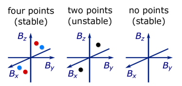
Figure 2: Magnetic degeneracy points for two interacting spin-1/2 electrons, when the relative sign of the $g$-tensors is negative, ${\cal S}=-1$. Color of each point indicates its topological charge: $+1$ (red), $-1$ (blue), 0 (black). Four points and no points patterns are stable, and the generic transition between them is that the two oppositely charged pairs meet and their charges annihilate each other (two points).

In this case, we find two stable eigenpatterns with codimension $d=0$, eigenpatterns (VIII) and (XI). Pattern (XI) corresponds to the trivial case, with no magnetic degeneracy at any field, while pattern (VIII) to the case of having two positively charged and two negatively charged Weyl points. One of the important messages of Table 2 is that there is no other stable configuration. The almost stable eigenpattern (X) of two chargeless degeneracy points is the generic pattern, separating extended regions (VIII) and (XI) of stable configurations in parameter space. These are precisely the points at which two oppositely charged Weyl points merge and annihilate each other, see Fig. 2. The remaining eigenpattern (IX) corresponds to a loop of magnetic degeneracy points and, with codimension $d=3$, is very unstable.

V Conclusions

In conclusion, we have provided a full analytical description of the geometrical patterns and topological charge distribution patterns of magnetic ground-state degeneracy points in a spin-orbit-coupled two-spin system. By recognizing the special structure of the Hamiltonian, we have mapped the problem of finding the denegeracy points to the eigenproblem of a real non-symmetric $3\times 3$ matrix. We have found three drastically different regions in parameter space, according to the total topological charge in magnetic space, ${\cal Q}=\text{sgn}(\text{det}\,\hat{\text{\boldmath{$g$}}}_{\text{L}})+\text{sgn}(\text{det}\,\hat{\text{\boldmath{$g$}}}_{\text{R}})$.

The regions ${\cal Q}=\pm 2$ are very similar, only the signs of the charge distributions are the opposite. In both regions, our stability analysis reveals the existence of two stable and extended (i.e., non-zero measure) regions in the secondary parameter space: in the first one, case (VII), two magnetic Weyl points carry the topological charge, while in the second one, case (I), six Weyl points carry the total charge, ${\cal Q}=4\times(+1)+2\times(-1)$. There is no other geometrically stable region, meaning that other charge patterns exist only in special, fine-tuned Hamiltonians, realized for secondary parameters forming a set of zero measure. Some of these configurations can, however, be observed. For ${\cal Q}=+2$, for instance, the most stable unstable structure, the one with two merged Weyl points, that is, when $\text{ep}(\hat{\text{\boldmath{$M$}}})=$ (III), emerges at the boundary between the two topologically stable phases, (I) and (VII). We naturally cross this surface in case we change some of the secondary parameters of the Hamiltonian, such that we go continuously from a region with $\text{ep}(\hat{\text{\boldmath{$M$}}})=$(I) to a region with $\text{ep}(\hat{\text{\boldmath{$M$}}})=$(VII). Approaching this surface, a positively and negatively charged pair of Weyl points must approach each other, and just merge to annihilate each other. This boundary, corresponding to $\text{ep}(\hat{\text{\boldmath{$M$}}})=$(III), includes further special patterns, corresponding to further fine-tuning of the parameters.

A similar picture emerges for the case ${\cal Q}=0$. There, two generic, extended regions are found with no degeneracy points ($\text{ep}(\hat{\text{\boldmath{$M$}}})=$(XI)), and with four Weyl points ($\text{ep}(\hat{\text{\boldmath{$M$}}})=$(VIII)), respectively. The generic surface between them corresponds to $\text{ep}(\hat{\text{\boldmath{$M$}}})=$(X), with two neutral degeneracy points, where the two pairs of Weyl points just merged. These magnetic degeneracy patterns are shown in Fig. 2.

The linear stability of regions (I), (VII), (VIII) and (XI) is corroborated by robust topological arguments: Weyl points cannot disappear upon infinitesimal smooth deformations of the secondary parameters. Starting from these configurations, removing Weyl points or creating new degeneracy points requires fine-tuning of the parameters: either positive and negative charges must move towards each other, and then annihilate at a very special point (this corresponds to the boundaries (III) and (X) discussed above), or fine-tuning leads to the formation of an ellipse or an ellipsoid of degeneracy points that are not Weyl points, as their energy dispersion is flat in at least one direction. Numbers and charges of the Weyl points in regions (I), (VII), (VIII) and (XI) are constrained by the total topological charge, whereas the relative locations of these Weyl points is constrained by the fact that they always come in time-reversed pairs.Scherübl et al. (2019)

The classification problem studied here is readily generalized to any interacting spin system, e.g., three interacting electrons subject to spin-orbit coupling, or two interacting spins with larger spin size. Studying possible geometrical patterns of the magnetic degeneracy points, the corresponding topological charge density patterns, the stability of these and their evolution upon continuous deformations of the Hamiltonian are interesting and challenging tasks.

A further direction for generalization is to analyze magnetic degeneracy points of higher-energy eigenstates instead of the ground stateBruno (2006). An interesting set of further problems is obtained if the spin-orbit effects are not completely arbitrary, but are subject to symmetry constraints. For example, if magnetic adatoms are placed on specific sites on a metallic surfaceWiesendanger (2009); Spinelli et al. (2015), then the spatial symmetry of the arrangement will restrict the form of the $g$-tensors and the exchange terms. In general, a fully numerical approach can provide insight into the questions above, but it seems difficult to efficiently generalize the analytical treatment used here to obtain exact results for a much broader set of physically motivated Hamiltonians.

Besides opening up interesting theory questions, we hope that our work will inspire experiments as well. Weyl points in interacting spin systems have been found experimentally by transportScherübl et al. (2019) and Landau-Zener spectroscopyWernsdorfer and Sessoli (1999), but their topological characterization, e.g., via measurements of the Berry curvatureGritsev and Polkovnikov (2012); Roushan et al. (2014), is yet to be done. To observe a sharp transition between different eigenpatters studied here, e.g., to observe creation and annihilation of Weyl points, the experimenter needs exquisite control over the $g$-tensors and spin-spin interaction. This is given, to some extent, in spin-orbit-coupled quantum dotsCsonka et al. (2008); Veldhorst et al. (2015), but a fruitful alternative realization could be done in superconducting qubits, where synthetic qubit-qubit interaction, including antisymmetric exchangeWang et al. (2019), can be engineered and controlled.

Appendix A Survival kit for the eigenvalue problem of non-symmetric real matrices

Quantum physicists are very familiar with the eigenvalue problem of symmetric real matrices and Hermitian complex matrices, but less familiar with the eigenproblem of real non-symmetric matrices. Therefore, here we summarize a few useful concepts and relations about the latter.

For concreteness, we consider a $3\times 3$ real non-symmetric matrix $\hat{\text{\boldmath{$M$}}}$, as in the main text. The complex number $\lambda$ is an eigenvector of $\hat{\text{\boldmath{$M$}}}$, if $\text{det}(\hat{\text{\boldmath{$M$}}}-\lambda\mathds{1})=0$. All eigenvalues of a real symmetric matrix are real, but this is not guaranteed if the matrix is non-symmetric. The quantity $\text{det}(\hat{\text{\boldmath{$M$}}}-\lambda\mathds{1})$ is called the characteristic polynomial of $\hat{\text{\boldmath{$M$}}}$. According to the fundamental theorem of algebra, the characteristic polynomial can be factored into the product of 3 terms,

$$\text{det}(\hat{\text{\boldmath{$M$}}}-\lambda\mathds{1})=(\lambda_{1}-\lambda)(\lambda_{2}-\lambda)(\lambda_{3}-\lambda),$$ (23)

where $\lambda_{i}$-s are the eigenvalues of $\hat{\text{\boldmath{$M$}}}$.

The algebraic multiplicity $\mu(\lambda_{i})$ of the eigenvalue $\lambda_{i}$ is its multiplicity as a root of the characteristic polynomial. The geometric multiplicity $\gamma(\lambda_{i})$ is the maximal number of linearly independent eigenvectors belonging to the eigenvalue $\lambda_{i}$, that is, the dimension of the eigensubspace corresponding to $\lambda_{i}$. For generic $3\times 3$ matrices, it holds that $1\leq\gamma(\lambda_{i})\leq\mu(\lambda_{i})\leq 3$, while for real symmetric and complex Hermitian matrices, it holds that $1\leq\gamma(\lambda_{i})=\mu(\lambda_{i})\leq 3$.

A real symmetric (complex Hermitian) matrix can always be diagonalized with an orthogonal (unitary) transformation, whose matrix is constructed from the eigenvectors. This is not the case for a real non-symmetric matrix. Nevertheless, there is still a canonical form $\hat{\text{\boldmath{$J$}}}$ of a real non-symmetric matrix $\hat{\text{\boldmath{$M$}}}$, called the Jordan normal form, see the examples in Table 1. The Jordan normal form is not diagonal, but it has a block-diagonal structure, and this structure is related to the algebraic and geometrical multiplicities of $\hat{\text{\boldmath{$M$}}}$. If the matrix has a size greater than 3, then the eigenvalues and their algebraic and geometric multiplicities are in general not sufficient to determine the Jordan normal form of the matrix. But in our case, when $\hat{\text{\boldmath{$M$}}}$ is a $3\times 3$ matrix, the eigenvalues and the multiplicities do determine the Jordan normal form: each eigenvalue $\lambda_{i}$ has a block in the Jordan normal form with the size of its algebraic multiplicity $\mu(\lambda_{i})$, and within each block, there are as many 1 entries on the superdiagonal as the difference $\mu(\lambda_{i})-\gamma(\lambda_{i})$ between the algebraic and geometric multiplicities. In Table 1, we list 7 examples. The claim is that for any matrix $\hat{\text{\boldmath{$M$}}}$, there is a similarity transformation (invertible matrix) $\hat{\text{\boldmath{$P$}}}$, such that

$$\hat{\text{\boldmath{$J$}}}=\hat{\text{\boldmath{$P$}}}^{-1}\hat{\text{\boldmath{$M$}}}\hat{\text{\boldmath{$P$}}}$$ (24)

is a Jordan normal form, and hence any matrix $\hat{\text{\boldmath{$M$}}}$ can be decomposed as in Eq. (7).

Appendix B The role of local spin basis transformations

Here, we collect a few facts and remarks about the role of local spin basis transformations in the spin-orbit-coupled two-spin problem studied in the main text. Some of these are used in our proofs.

Existence of a basis where the $g$-tensors are symmetric. The Hamiltonian in Eq. (1) is built on a single-particle modelScherübl et al. (2019) in which both sites support a single spinful orbital level, and the corresponding two states are Kramers degenerate at zero magnetic field. Because of this Kramers degeneracy, there is an ambiguity in choosing the basis states. The Hamiltonian in Eq. (1) is generic, i.e., this form is guaranteed no matter how we choose the basis. However, the actual secondary parameters ($g$-tensor matrix elements and the rotation matrix $\hat{\text{\boldmath{$R$}}}$) change if we change the basis.

First, we show that one can always choose a local spin basis in which the $g$-tensors are symmetric. For this, we recall that any local spin basis transformation, apart from an arbitrary complex phase, can be written as a unitary operationDiósi (2007)

$$U(\text{\boldmath{$\alpha$}})=\exp\left(-i\text{\boldmath{$\alpha$}}\text{\boldmath{$S$}}\right),$$ (25)

where $\alpha$ is a real three-component vector. Furthermore, this transformation corresponds to a rotation $\hat{\text{\boldmath{$O$}}}_{\text{\boldmath{$\alpha$}}}$ of the spin vector operator around the direction of $\alpha$ with angle $\alpha=|\text{\boldmath{$\alpha$}}|$:

$$U(\text{\boldmath{$\alpha$}})\text{\boldmath{$S$}}U(\text{\boldmath{$\alpha$}})^{\dagger}=\hat{\text{\boldmath{$O$}}}_{\text{\boldmath{$\alpha$}}}\text{\boldmath{$S$}}.$$ (26)

When we apply two different transformations on the two sites, $U_{\text{L}}$ and $U_{\text{R}}$, which are represented by the rotations $\hat{\text{\boldmath{$O$}}}_{\text{L}}$ and $\hat{\text{\boldmath{$O$}}}_{\text{R}}$, respectively, then this combined transformation results in

$$H^{\prime} = (U_{\text{L}}\otimes U_{\text{R}})H(U_{\text{L}}\otimes U_{\text{R}})^{\dagger}$$ (27)

$$= \mu_{\text{B}}\text{\boldmath{$B$}}(\hat{\text{\boldmath{$g$}}}_{\text{L}}\hat{\text{\boldmath{$O$}}}_{\text{L}}\text{\boldmath{$S$}}_{\text{L}}+\hat{\text{\boldmath{$g$}}}_{\text{R}}\hat{\text{\boldmath{$O$}}}_{\text{R}}\text{\boldmath{$S$}}_{\text{R}})+$$

$$+ J\text{\boldmath{$S$}}_{\text{L}}\hat{\text{\boldmath{$O$}}}_{\text{L}}^{-1}\hat{\text{\boldmath{$R$}}}\hat{\text{\boldmath{$O$}}}_{\text{R}}\text{\boldmath{$S$}}_{\text{R}}.$$

Recall also that any real symmetric matrix has a polar decomposition to a symmetric real matrix and a rotation matrix, therefore the $g$-tensors can also be decomposed as $\hat{\text{\boldmath{$g$}}}_{\text{L/R}}=\hat{\text{\boldmath{$G$}}}_{\text{L/R}}\hat{\text{\boldmath{$Q$}}}_{\text{L/R}}$, where $\hat{\text{\boldmath{$G$}}}_{\text{L/R}}$ are real and symmetric and $\hat{\text{\boldmath{$Q$}}}_{\text{L/R}}$ are rotations. Therefore, by using the basis transformation as $\hat{\text{\boldmath{$O$}}}_{\text{L/R}}=\hat{\text{\boldmath{$Q$}}}_{\text{L/R}}^{-1}$, the transformed Hamiltonian reads

$$H^{\prime} = \mu_{\text{B}}\text{\boldmath{$B$}}(\hat{\text{\boldmath{$G$}}}_{\text{L}}\text{\boldmath{$S$}}_{\text{L}}+\hat{\text{\boldmath{$G$}}}_{\text{R}}\text{\boldmath{$S$}}_{\text{R}})+$$ (28)

$$+ J\text{\boldmath{$S$}}_{\text{L}}\hat{\text{\boldmath{$R$}}}^{\prime}\text{\boldmath{$S$}}_{\text{R}}.$$

An interesting feature of this particular basis choice is its strong relevance to spectroscopy experiments: if a spectroscopy experiment measures the Zeeman splitting as a function of the magnetic field direction, then the principal axes and principal values of $\hat{\text{\boldmath{$G$}}}$ can be directly calculated from that data.Crippa et al. (2018) Another interesting feature of this basis is that in the limit of small exchange rotation, $\hat{\text{\boldmath{$R$}}}\rightarrow\mathds{1}$, the degeneracy points always form the ‘six-point’ pattern, due to the fact that the matrix $\hat{\text{\boldmath{$M$}}}$ converges to a real matrix that has only positive eigenvalues.

$\hat{\text{\boldmath{$M$}}}$ is invariant under any local spin transformation. In the main text, we have used the matrix $\hat{M}$ to characterize the magnetic degeneracy points. It is a natural expectation that the locations of the degeneracy points do not depend on the local spin basis choice. Can we prove this directly? Yes, and actually we can prove something stronger: the matrix $\hat{M}$ itself is invariant under local spin basis transformations. This is a straightforward consequence of the transformation rules used above. A general basis transformation results in $\hat{\text{\boldmath{$g$}}}_{\text{L/R}}\mapsto\hat{\text{\boldmath{$g$}}}_{\text{L,R}}\hat{\text{\boldmath{$O$}}}_{\text{L,R}}$ and $\hat{\text{\boldmath{$R$}}}\mapsto\hat{\text{\boldmath{$O$}}}_{\text{L}}^{-1}\hat{\text{\boldmath{$R$}}}\hat{\text{\boldmath{$O$}}}_{\text{R}}$. Substituting these into the definition of $\hat{\text{\boldmath{$M$}}}$ we can get the transformed matrix as

$$\hat{\text{\boldmath{$M$}}}\mapsto(\hat{\text{\boldmath{$g$}}}_{\text{L}}\hat{\text{\boldmath{$O$}}}_{\text{L}})(\hat{\text{\boldmath{$O$}}}_{\text{L}}^{-1}\hat{\text{\boldmath{$R$}}}\hat{\text{\boldmath{$O$}}}_{\text{R}})(\hat{\text{\boldmath{$O$}}}_{\text{R}}^{-1}\hat{\text{\boldmath{$g$}}}_{\text{R}}^{-1})=\hat{\text{\boldmath{$M$}}},$$ (29)

so $\hat{\text{\boldmath{$M$}}}$ is indeed invariant under local spin transformations as we expected.

Appendix C Locations of the magnetic degeneracy points

Here, we outline how to determine the locations of the ground-state magnetic degeneracy points studied in the main text.

First, we consider the case when the magnetic field vector $\text{\boldmath{$B$}}=B\text{\boldmath{$v$}}_{a}$ is a left eigenvector of $\hat{\text{\boldmath{$M$}}}$ with a positive eigenvalue $a$, and we assume that $\text{\boldmath{$v$}}_{a}$ is normalized. Then, the effective magnetic field vectors of Eq. (4) are parallel, $\text{\boldmath{$B$}}_{\text{L,eff}}\parallel\text{\boldmath{$B$}}_{\text{R,eff}}$, and point to the same direction. Using that direction as the spin quantization axis, the Hamiltonian defined in Eq. (4) has a special form

$$H^{\prime}=\mu_{\text{B}}B(g_{\text{L}}S^{\prime}_{\text{L}z}+g_{\text{R}}S^{\prime}_{\text{R}z})+J\text{\boldmath{$S$}}^{\prime}_{\text{L}}\cdot\text{\boldmath{$S$}}^{\prime}_{\text{R}},$$ (30)

where $g_{\text{L,R}}=|\text{\boldmath{$v$}}_{a}\hat{\text{\boldmath{$g$}}}_{\text{L,R}}|$. Later we will use the fact that

$$g_{\text{L}}/g_{\text{R}}=a,$$ (31)

which follows from $\text{\boldmath{$v$}}_{a}$ being a left eigenvector of $\hat{\text{\boldmath{$M$}}}$ with eigenvalue $a$. This Hamiltonian $H^{\prime}$ conserves the total spin projection $S_{z}^{\prime}=S_{\text{L}z}^{\prime}+S_{\text{R}z}^{\prime}$, and thus has the following block-diagonal matrix form in the product basis $\ket{\uparrow\uparrow}$, $\ket{\uparrow\downarrow}$, $\ket{\downarrow\uparrow}$, $\ket{\downarrow\downarrow}$:

$$H^{\prime}=\frac{1}{2}\begin{pmatrix}\mu_{\text{B}}g_{+}B&0&0&0\\ 0&\mu_{\text{B}}g_{-}B-J&J&0\\ 0&J&-\mu_{\text{B}}g_{-}B-J&0\\ 0&0&0&-\mu_{\text{B}}g_{+}B\\ \end{pmatrix},$$ (32)

where $g_{\pm}=g_{\text{L}}\pm g_{\text{R}}$. Energy eigenstates from different subspaces of $S_{z}^{\prime}$ can be degenerate, because there are no matrix elements mixing them.

At zero magnetic field, the ground state of $H^{\prime}$ in Eq. (32) is the singlet state $(\ket{\uparrow\downarrow}-\ket{\downarrow\uparrow})/\sqrt{2}$ from the $S_{z}^{\prime}=0$ subspace, with energy $-J$ , and the remaining three states are triplets with zero energy. If the magnetic field is much greater than the interaction strength $J$, then the energy eigenstates are the product states. The ground state is the state $\ket{\downarrow\downarrow}$ from the $S_{z}^{\prime}=-1$ subspace with energy $-\frac{1}{2}\mu_{\text{B}}g_{+}B$: this follows from that fact that $|g_{+}|>|g_{-}|$, which is implied by $g_{\text{L}},g_{\text{R}}>0$. Therefore, at a certain magnetic field strength between zero and infinity, the $S_{z}^{\prime}=0$ ground state must be degenerate with the $S_{z}^{\prime}=-1$ ground state. In fact, straightforward calculation shows that this level crossing degeneracy happens at the critical magnetic field strength

$$B_{a}=\frac{J}{2\mu_{B}}\left(\frac{1}{g_{\text{L}}}+\frac{1}{g_{\text{R}}}\right),$$ (33)

and the degenerate ground states are

$$\ket{0} = \frac{1}{\sqrt{g_{\text{L}}^{2}+g_{\text{R}}^{2}}}(g_{\text{R}}\ket{\uparrow\downarrow}-g_{\text{L}}\ket{\downarrow\uparrow})$$ (34a)

$$\ket{-1} = \ket{\downarrow\downarrow}$$ (34b)

labelled with their $S^{\prime}_{z}$ quantum number.

If, on the other hand, $B$ is a left eigenvector of $\hat{\text{\boldmath{$M$}}}$ with a negative eigenvalue, then the effective magnetic fields $\text{\boldmath{$B$}}_{\text{L,eff}}$ and $\text{\boldmath{$B$}}_{\text{R,eff}}$ are anti-aligned. Then, the Hamiltonian can be brought to the same form as in Eq. (32), with the change that now $|g_{+}|<|g_{-}|$. Therefore, the ground states in the limits of zero and large magnetic fields are both in the $S_{z}^{\prime}=0$ subspace, and there is no ground-state level crossing.

Appendix D Closed degeneracy lines are ellipses, closed degeneracy surfaces are ellipsoids

In Table 1, the eigenpattern (IV) implies that the degeneracy points form a closed surface. Here we show that this surface is an ellipsoid. A similar proof shows that the loops formed by the degeneracy points in cases (II), (V), and (X) are ellipses.

In case (IV), the matrix $\hat{\text{\boldmath{$M$}}}$ has a single eigenvalue $a$ and the normalized eigenvectors form the three-dimensional unit sphere. So, any $v$ unit vector is an eigenvector, and we can apply the results (31) and (33) to obtain the locations of the degeneracy points

$$\text{\boldmath{$B$}}_{a}(\text{\boldmath{$v$}})=\frac{J(1+a)}{2\mu_{\text{B}}}\frac{\text{\boldmath{$v$}}}{|\text{\boldmath{$v$}}\hat{\text{\boldmath{$g$}}}_{\text{L}}|}=\frac{J(1+a)}{2\mu_{\text{B}}}\frac{\text{\boldmath{$v$}}}{|\text{\boldmath{$v$}}\hat{\text{\boldmath{$G$}}}_{\text{L}}|}.$$ (35)

In the second step, we have made use of the polar decomposition of $\hat{\text{\boldmath{$g$}}}_{\text{L}}$, introduced in Appendix B, where $\hat{\text{\boldmath{$G$}}}_{\text{L}}$ denotes the real symmetric component. In the principal reference frame of $\hat{\text{\boldmath{$G$}}}_{\text{L}}$, the location of the degeneracy point associated to $v$ reads

$$\left(\begin{array}[]{c}B_{ax}\\ B_{ay}\\ B_{az}\end{array}\right)=\frac{J(1+a)}{2\mu_{\text{B}}}\frac{1}{\sqrt{G_{x}^{2}v_{x}^{2}+G_{y}^{2}v_{y}^{2}+G_{z}^{2}v_{z}^{2}}}\left(\begin{array}[]{c}v_{x}\\ v_{y}\\ v_{z}\end{array}\right),$$ (42)

where $(G_{x},G_{y},G_{z})$ are the principal values of $\hat{\text{\boldmath{$G$}}}_{\text{L}}$. Acting with $\hat{\text{\boldmath{$G$}}}_{\text{L}}$ on both sides of the equation, and taking the length-squared of the resulting vectors, we obtain the equation

$$G_{x}^{2}B_{ax}^{2}+G_{y}^{2}B_{ay}^{2}+G_{z}^{2}B_{az}^{2}=\left[\frac{J(1+a)}{2\mu_{\text{B}}}\right]^{2},$$ (43)

which implies that the degeneracy points form an ellipsoid.

For cases (II), (V), and (X), we have an additional constraint: $v$ has to be in the degenerate subspace of $\hat{\text{\boldmath{$M$}}}$. This intersects the ellipsoid with a plane passing through the origin. Since the intersection of a plane and an ellipsoid is always an ellipse, we conclude that the degeneracy points in these cases are ellipses.

Appendix E Topological charge distributions

Here, we outline the derivation of the topological charges associated to the ground-state magnetic degeneracy points. The results were summarized in Tables 1 and 2 in the main text. The first, simple step of the derivation is to approximate the Hamiltonian in the vicinity of the degeneracy point and truncate it to the two-dimensional degerate subspace of interest. A second, nontrivial step is to connect this two-dimensional Hamiltonian to the eigenvalue problem of the matrix $\hat{\text{\boldmath{$M$}}}$, which allows us to express the topological charges of the degeneracy points via the eigenvalues of $\hat{\text{\boldmath{$M$}}}$.

To exemplify the derivation, consider the case when the total topological charge is ${\cal Q}=+2$, and the eigenpattern of $\hat{\text{\boldmath{$M$}}}$ is (I) (see Table 1). Then $\hat{\text{\boldmath{$M$}}}$ has three eigenvalues $a$, $b$, $c$, three eigenvectors $\text{\boldmath{$v$}}_{a}$, $\text{\boldmath{$v$}}_{b}$, $\text{\boldmath{$v$}}_{c}$, and the set of the ground-state magnetic degeneracy points is formed by six Weyl points. To calculate the topological charge of a Weyl point, say, $\text{\boldmath{$B$}}_{a+}$, we focus on the two degenerate ground states $\ket{0}$ and $\ket{-1}$ in the degeneracy point (see Eqs. (34)), make a linear expansion of the Hamiltonian for small deviations $\delta\text{\boldmath{$B$}}=\text{\boldmath{$B$}}-\text{\boldmath{$B$}}_{a+}$ of the magnetic field from the degeneracy point, and truncate the Hamiltonian for the two-dimensional subspace spanned by $\ket{0}$ and $\ket{-1}$. This reduced Hamiltonian can be written in terms of Pauli matrices,

$$H_{\text{red}}(\delta\text{\boldmath{$B$}})=\mu_{\text{B}}\,\delta\!\text{\boldmath{$B$}}\,\hat{\text{\boldmath{$g$}}}_{a+}\text{\boldmath{$\tau$}},$$ (44)

where $\text{\boldmath{$\tau$}}=(\tau_{1},\tau_{2},\tau_{3})$ is half times the vector of Pauli matrices, e.g., $\tau_{3}=\frac{1}{2}(\ket{0}\bra{0}-\ket{-1}\bra{-1})$. Because of the similarity of $H_{\text{red}}$ and the Hamiltonian of a spin in a magnetic field with an anisotropic $g$-tensor, we call $\hat{\text{\boldmath{$g$}}}_{a+}$ the effective $g$-tensor of the degeneracy point $\text{\boldmath{$B$}}_{a+}$. The determinant of effective $g$-tensor of a Weyl point is nonzero, and its sign provides the topological charge of the Weyl point:

$$\mathcal{Q}_{a+}=\text{sgn}\,\text{det}\left(\hat{\text{\boldmath{$g$}}}_{a+}\right).$$ (45)

To obtain an analytical result for the elements of the effective $g$-tensor, we evaluate $H_{\text{red}}$ in Eq. (44) with $\delta\text{\boldmath{$B$}}=\delta B\text{\boldmath{$e$}}_{\alpha}$ ($\alpha=x,y,z$) pointing along the unit vector $\text{\boldmath{$e$}}_{\alpha}$ of direction $\alpha$, multiply both sides with $\tau_{\beta}$ ($\beta=x,y,z$), and take the trace of both sides. This procedure yields the matrix elements

$$(\hat{\text{\boldmath{$g$}}}_{a+})_{\alpha\beta}=\frac{2}{\mu_{\text{B}}\delta B}\text{Tr}[H_{\text{red}}(\delta B\,\text{\boldmath{$e$}}_{\alpha})\cdot\tau_{\beta}].$$ (46)

The matrix obtained from this relation can be identified with this expression:

$$\begin{split}\hat{\text{\boldmath{$g$}}}_{a+}=&\frac{g^{2}_{\text{R}}\hat{\text{\boldmath{$g$}}}_{\text{L}}+g^{2}_{\text{L}}\hat{\text{\boldmath{$g$}}}_{\text{R}}\hat{\text{\boldmath{$R$}}}^{-1}}{g^{2}_{\text{L}}+g^{2}_{\text{R}}}\text{\boldmath{$e$}}_{z}\otimes\text{\boldmath{$e$}}_{z}+\\ &\frac{g_{\text{R}}\hat{\text{\boldmath{$g$}}}_{\text{L}}-g_{\text{L}}\hat{\text{\boldmath{$g$}}}_{\text{R}}\hat{\text{\boldmath{$R$}}}^{-1}}{\sqrt{g^{2}_{\text{L}}+g^{2}_{\text{R}}}}(\mathds{1}-\text{\boldmath{$e$}}_{z}\otimes\text{\boldmath{$e$}}_{z}).\end{split}$$ (47)

Here, $\otimes$ denotes the dyadic product.

The determinant of (47) can expressed with the eigenvalues of the matrix $\hat{\text{\boldmath{$M$}}}$, yielding

$$\det\hat{\text{\boldmath{$g$}}}_{a+}=\frac{a(1+a)}{(1+a^{2})^{2}}(a-b)(a-c)\det\hat{\text{\boldmath{$g$}}}_{\text{R}},$$ (48)

Inserting this determinant into Eq. (46) and using $a>0$ and $\text{det}\,\hat{\text{\boldmath{$g$}}}_{\text{R}}>0$, we obtain

$${\cal Q}_{a+}=\text{sgn}[(a-b)(a-c)].$$ (49)

The same result is obtained for ${\cal Q}_{a-}$, and analogous results are obtained for the remaining four degeneracy points, e.g.,

$${\cal Q}_{b+}=\text{sgn}[(b-a)(b-c)].$$ (50)

These results imply that for the eigenpattern (I), the distribution of topological charge among the six degeneracy points is $4\times(+1),\ 2\times(-1)$, and that the negatively charged point pair belongs to the eigenvalue that is between the other two eigenvalues.

For the eigenpatterns (II) and (III), the two Weyl points belonging to the non-degenerate eigenvalue $b$ can be analyzed in an analogous fashion, with the result that their topological charge is $+1$. As a natural consequence of this and the sum rule that the total topological charge is +2, the remaining degeneracy points, that is, the ellipse in case (II) and the two remaining points in case (III), must have zero topological charge. For the remaining eigenpatterns from (III) to (VII), the distribution of the total topological charge $+2$ is obvious.

We note that the result (48) is valid not only for Weyl points but for any ground-state magnetic degeneracy point. This has interesting implications regarding the energy dispersion in the vicinity of a degeneracy point $\text{\boldmath{$B$}}_{a+}$ whenever that point is in an eigenspace of $\hat{\text{\boldmath{$M$}}}$ that belongs to a degenerate eigenvalue $a$. In that case, the degeneracy of $a$ implies that the right hand side of (48) yields zero, i.e., there is at least one direction for $\delta\text{\boldmath{$B$}}$ along which the dispersion is non-linear. In cases (II), (IV), (V) and (IX), naturally, the special non-dispersive directions are the tangents of the ellipse and the ellipsoid. However, it is remarkable that discrete degeneracy points can also have non-linear dispersion. Examples are the two points in case (VI) with non-zero charge and the neutral points in cases (III) and (X). Degeneracy points showing similar non-linear dispersion are sometimes called multi-Weyl pointsFang et al. (2012); Yan and Wang (2017); Ahn et al. (2017); Huang et al. (2017) in the literature. In general, their topological charges cannot be determined by their effective $g$-tensor: for example, in case (VI), the determinants of the effective $g$-tensors of the two degeneracy points are zero, nevertheless each point has a topological charge $+1$.

References

- Wernsdorfer and Sessoli (1999) W. Wernsdorfer and R. Sessoli, “Quantum phase interference and parity effects in magnetic molecular clusters,” Science 284, 133–135 (1999).
- Garg (2010) Anupam Garg, “Berry phases near degeneracies: Beyond the simplest case,” Am. J. Phys. 78, 661 (2010).
- Bruno (2006) Patrick Bruno, “Berry phase, topology, and degeneracies in quantum nanomagnets,” Phys. Rev. Lett. 96, 117208 (2006).
- Wiesendanger (2009) Roland Wiesendanger, “Spin mapping at the nanoscale and atomic scale,” Rev. Mod. Phys. 81, 1495–1550 (2009).
- Spinelli et al. (2015) A. Spinelli, M. Gerrits, R. Toskovic, B. Bryant, M. Ternes, and A. F. Otte, “Exploring the phase diagram of the two-impurity kondo problem,” Nature Communications 6, 10046 (2015).
- Hanson et al. (2007) R. Hanson, L. P. Kouwenhoven, J. R. Petta, S. Tarucha, and L. M. K. Vandersypen, “Spins in few-electron quantum dots,” Rev. Mod. Phys. 79, 1217–1265 (2007).
- Zwanenburg et al. (2013) Floris A. Zwanenburg, Andrew S. Dzurak, Andrea Morello, Michelle Y. Simmons, Lloyd C. L. Hollenberg, Gerhard Klimeck, Sven Rogge, Susan N. Coppersmith, and Mark A. Eriksson, “Silicon quantum electronics,” Rev. Mod. Phys. 85, 961–1019 (2013).
- Berry (1984) M. V. Berry, “Quantal phase factors accompanying adiabatic changes,” 392, 45–57 (1984).
- Wilczek and Shapere (1989) Frank Wilczek and Alfred Shapere, Geometric phases in physics, Vol. 5 (World Scientific, 1989).
- San-Jose et al. (2008) Pablo San-Jose, Burkhard Scharfenberger, Gerd Schön, Alexander Shnirman, and Gergely Zarand, “Geometric phases in semiconductor spin qubits: Manipulations and decoherence,” Phys. Rev. B 77, 045305 (2008).
- San-Jose et al. (2006) Pablo San-Jose, Gergely Zarand, Alexander Shnirman, and Gerd Schön, “Geometrical spin dephasing in quantum dots,” Phys. Rev. Lett. 97, 076803 (2006).
- Klitzing et al. (1980) K. v. Klitzing, G. Dorda, and M. Pepper, “New Method for High-Accuracy Determination of the Fine-Structure Constant Based on Quantized Hall Resistance,” Phys. Rev. Lett. 45, 494–497 (1980).
- Thouless, D. J. and Kohmoto, M. and Nightingale, M. P. and den Nijs, M. (1982) Thouless, D. J. and Kohmoto, M. and Nightingale, M. P. and den Nijs, M., “Quantized hall conductance in a two-dimensional periodic potential,” Phys. Rev. Lett. 49, 405–408 (1982).
- (14) J. von Neumann and E. P. Wigner, “Über das Verhalten von Eigenwerten bei adiabatischen Prozessen,” Physikalische Zeitschrift 30, 467.
- Herring (1937) Conyers Herring, “Accidental degeneracy in the energy bands of crystals,” Phys. Rev. 52, 365–373 (1937).
- Gritsev and Polkovnikov (2012) V. Gritsev and A. Polkovnikov, “Dynamical quantum Hall effect in the parameter space,” Proceedings of the National Academy of Sciences 109, 6457–6462 (2012).
- Roushan et al. (2014) P. Roushan, C. Neill, Yu Chen, M. Kolodrubetz, C. Quintana, N. Leung, M. Fang, R. Barends, B. Campbell, Z. Chen, B. Chiaro, A. Dunsworth, E. Jeffrey, J. Kelly, A. Megrant, J. Mutus, P. J. J. O’Malley, D. Sank, A. Vainsencher, J. Wenner, T. White, A. Polkovnikov, A. N. Cleland, and J. M. Martinis, “Observation of topological transitions in interacting quantum circuits,” Nature 515, 241 (2014).
- Scherübl et al. (2019) Zoltán Scherübl, András Pályi, György Frank, István Endre Lukács, Gergő Fülöp, Bálint Fülöp, Jesper Nygård, Kenji Watanabe, Takashi Taniguchi, Gergely Zaránd, and Szabolcs Csonka, “Observation of spin–orbit coupling induced weyl points in a two-electron double quantum dot,” Communications Physics 2, 108 (2019).
- Armitage et al. (2018) N. P. Armitage, E. J. Mele, and Ashvin Vishwanath, “Weyl and Dirac semimetals in three-dimensional solids,” Rev. Mod. Phys. 90, 015001 (2018).
- Riwar et al. (2016) Roman-Pascal Riwar, Manuel Houzet, Julia S. Meyer, and Yuli V. Nazarov, “Multi-terminal josephson junctions as topological matter,” Nature Communications 7, 11167 (2016).
- Stenger and Pekker (2019) John P. T. Stenger and David Pekker, “Weyl points in systems of multiple semiconductor-superconductor quantum dots,” Phys. Rev. B 100, 035420 (2019).
- Gao et al. (2016) Wenlong Gao, Biao Yang, Mark Lawrence, Fengzhou Fang, Benjamin Béri, and Shuang Zhang, “Photonic weyl degeneracies in magnetized plasma,” Nature Communications 7, 12435 (2016).
- Kavokin (2004) K. V. Kavokin, “Symmetry of anisotropic exchange interactions in semiconductor nanostructures,” Phys. Rev. B 69, 075302 (2004).
- Nowack et al. (2007) K. C. Nowack, F. H. L. Koppens, Yu. V. Nazarov, and L. M. K. Vandersypen, “Coherent control of a single electron spin with electric fields,” Science 318, 1430–1433 (2007).
- Nadj-Perge et al. (2010) S. Nadj-Perge, S. M. Frolov, E. P. A. M. Bakkers, and L. P. Kouwenhoven, Nature 468, 1084 (2010).
- Nadj-Perge et al. (2012) S. Nadj-Perge, V. S. Pribiag, J. W. G. van den Berg, K. Zuo, S. R. Plissard, E. P. A. M. Bakkers, S. M. Frolov, and L. P. Kouwenhoven, “Spectroscopy of spin-orbit quantum bits in indium antimonide nanowires,” Phys. Rev. Lett. 108, 166801 (2012).
- Schroer et al. (2011) M. D. Schroer, K. D. Petersson, M. Jung, and J. R. Petta, “Field tuning the factor in inas nanowire double quantum dots,” Phys. Rev. Lett. 107, 176811 (2011).
- Harvey-Collard et al. (2019) Patrick Harvey-Collard, N. Tobias Jacobson, Chloé Bureau-Oxton, Ryan M. Jock, Vanita Srinivasa, Andrew M. Mounce, Daniel R. Ward, John M. Anderson, Ronald P. Manginell, Joel R. Wendt, Tammy Pluym, Michael P. Lilly, Dwight R. Luhman, Michel Pioro-Ladrière, and Malcolm S. Carroll, “Spin-orbit interactions for singlet-triplet qubits in silicon,” Phys. Rev. Lett. 122, 217702 (2019).
- Tanttu et al. (2019) Tuomo Tanttu, Bas Hensen, Kok Wai Chan, Chih Hwan Yang, Wister Wei Huang, Michael Fogarty, Fay Hudson, Kohei Itoh, Dimitrie Culcer, Arne Laucht, Andrea Morello, and Andrew Dzurak, “Controlling spin-orbit interactions in silicon quantum dots using magnetic field direction,” Phys. Rev. X 9, 021028 (2019).
- Guckenheimer and Holmes (1983) J. Guckenheimer and P. Holmes, Nonlinear Oscillations, Dynamical Systems, and Bifurcations of Vector Fields (Springer, 1983).
- Berry (2004) M. V. Berry, “Physics of nonhermitian degeneracies,” Czechoslovak Journal of Physics 54, 1039 (2004).
- Heiss (2012) W D Heiss, “The physics of exceptional points,” Journal of Physics A: Mathematical and Theoretical 45, 444016 (2012).
- Petta et al. (2005) J. R. Petta, A. C. Johnson, J. M. Taylor, E. A. Laird, A. Yacoby, M. D. Lukin, C. M. Marcus, M. P. Hanson, and A. C. Gossard, “Coherent manipulation of coupled electron spins in semiconductor quantum dots,” Science 309, 2180–2184 (2005), https://science.sciencemag.org/content/309/5744/2180.full.pdf .
- Reilly et al. (2008) D. J. Reilly, J. M. Taylor, J. R. Petta, C. M. Marcus, M. P. Hanson, and A. C. Gossard, “Suppressing spin qubit dephasing by nuclear state preparation,” Science 321, 817–821 (2008).
- Petta et al. (2010) J. R. Petta, H. Lu, and A. C. Gossard, “A coherent beam splitter for electronic spin states,” Science 327, 669–672 (2010).
- Fang et al. (2012) Chen Fang, Matthew J. Gilbert, Xi Dai, and B. Andrei Bernevig, “Multi-weyl topological semimetals stabilized by point group symmetry,” Phys. Rev. Lett. 108, 266802 (2012).
- Yan and Wang (2017) Zhongbo Yan and Zhong Wang, “Floquet multi-weyl points in crossing-nodal-line semimetals,” Phys. Rev. B 96, 041206 (2017).
- Ahn et al. (2017) Seongjin Ahn, E. J. Mele, and Hongki Min, “Optical conductivity of multi-weyl semimetals,” Phys. Rev. B 95, 161112 (2017).
- Huang et al. (2017) Ze-Min Huang, Jianhui Zhou, and Shun-Qing Shen, “Topological responses from chiral anomaly in multi-weyl semimetals,” Phys. Rev. B 96, 085201 (2017).
- Note (1) We can modify all elements of by changing some parameters of the original Hamiltonian.
- Csonka et al. (2008) S. Csonka, L. Hofstetter, F. Freitag, S. Oberholzer, C. Schönenberger, T. S. Jespersen, M. Aagesen, and J. Nygård, “Giant fluctuations and gate control of the g-factor in inas nanowire quantum dots,” Nano Letters 8, 3932–3935 (2008).
- Veldhorst et al. (2015) M. Veldhorst, R. Ruskov, C. H. Yang, J. C. C. Hwang, F. E. Hudson, M. E. Flatté, C. Tahan, K. M. Itoh, A. Morello, and A. S. Dzurak, “Spin-orbit coupling and operation of multivalley spin qubits,” Phys. Rev. B 92, 201401 (2015).
- Wang et al. (2019) Da-Wei Wang, Chao Song, Wei Feng, Han Cai, Da Xu, Hui Deng, Hekang Li, Dongning Zheng, Xiaobo Zhu, H. Wang, Shi-Yao Zhu, and Marlan O. Scully, “Synthesis of antisymmetric spin exchange interaction and chiral spin clusters in superconducting circuits,” Nature Physics 15, 382–386 (2019).
- Diósi (2007) Lajos Diósi, A Short Course in Quantum Information Theory: An Approach From Theoretical Physics (Springer-Verlag Berlin Heidelberg, 2007).
- Crippa et al. (2018) Alessandro Crippa, Romain Maurand, Léo Bourdet, Dharmraj Kotekar-Patil, Anthony Amisse, Xavier Jehl, Marc Sanquer, Romain Laviéville, Heorhii Bohuslavskyi, Louis Hutin, Sylvain Barraud, Maud Vinet, Yann-Michel Niquet, and Silvano De Franceschi, “Electrical spin driving by -matrix modulation in spin-orbit qubits,” Phys. Rev. Lett. 120, 137702 (2018).