Approximation-Refinement Testing of
Compute-Intensive Cyber-Physical Models:
An Approach Based on System Identification

Abstract.

Black-box testing has been extensively applied to test models of Cyber-Physical systems (CPS) since these models are not often amenable to static and symbolic testing and verification. Black-box testing, however, requires to execute the model under test for a large number of candidate test inputs. This poses a challenge for a large and practically-important category of CPS models, known as compute-intensive CPS (CI-CPS) models, where a single simulation may take hours to complete. We propose a novel approach, namely ARIsTEO, to enable effective and efficient testing of CI-CPS models. Our approach embeds black-box testing into an iterative approximation-refinement loop. At the start, some sampled inputs and outputs of the CI-CPS model under test are used to generate a surrogate model that is faster to execute and can be subjected to black-box testing. Any failure-revealing test identified for the surrogate model is checked on the original model. If spurious, the test results are used to refine the surrogate model to be tested again. Otherwise, the test reveals a valid failure. We evaluated ARIsTEO by comparing it with S-Taliro, an open-source and industry-strength tool for testing CPS models. Our results, obtained based on five publicly-available CPS models, show that, on average, ARIsTEO is able to find $24\%$ more requirements violations than S-Taliro and is $31\%$ faster than S-Taliro in finding those violations. We further assessed the effectiveness and efficiency of ARIsTEO on a large industrial case study from the satellite domain. In contrast to S-Taliro, ARIsTEO successfully tested two different versions of this model and could identify three requirements violations, requiring four hours, on average, for each violation.

1. Introduction

A common practice in the development of Cyber-Physical Systems (CPS) is to specify CPS behaviors using executable and dynamic models  (Liebel et al., 2018; Chowdhury et al., 2018; mat, 2019). These models support engineers in a number of activities, most notably in automated code generation and early testing and simulation of CPS. Recent technological advancements in the areas of robotics and autonomous systems have led to increasingly more complex CPS whose models are often characterized as compute-intensive (Chaturvedi, 2009; Arrieta et al., 2016, 2018; Sagardui et al., 2017; González et al., 2018). Compute-Intensive CPS models (CI-CPS) require a lot of computational power to execute (Arrieta et al., 2019) since they include complex computations such as dynamic, non-linear and non-algebraic mathematics, and further, they have to be executed for long durations in order to thoroughly exercise interactions between the CPS and its environment. For example, non-trivial simulations of an industrial model of a satellite system, capturing the satellite behavior for $24h$, takes on average around $84$ minutes (~1.5 hours) (Lux, 2019). The sheer amount of time required for just a single execution of CI-CPS models significantly impedes testing and verification of these models since many testing and verification strategies require to execute the Model Under Test (MUT) for hundreds or thousands of test inputs.

Approaches to verification and testing of CPS models can be largely classified into exhaustive verification, and white-box and black-box testing. Exhaustive verification approaches often translate CPS models into the input language of model checkers or Satisfiability Modulo Theories (SMT) solvers. CPS models, however, may contain constructs that cannot be easily encoded into the SMT solver input languages. For example, CPS models specified in the Simulink language (mat, 2019) allow importing arbitrary C code via S-Function blocks or include other plugins (e.g., the Deep Learning Toolbox (dee, 2019)). In addition, CPS models typically capture continuous dynamic and hybrid systems (Alur, 2015). Translating such modeling constructs into low-level logic-based languages is complex, has to be handled on a case-by case basis and may lead to loss of precision which may or may not be acceptable depending on the application domain. Furthermore, it is well-known that model checking such systems is in general undecidable (Henzinger et al., 1998; Alur et al., 1995; Alur, 2011). White-box testing uses the internal structure of the model under test to specifically choose inputs that exercise different paths through the model. Most white-box testing techniques aim to generate a set of test cases that satisfy some structural coverage criteria (e.g., (Julius et al., 2007; Dang and Nahhal, 2009)). To achieve their intended coverage goals, they may rely either on SMT-solvers (e.g., (Kong et al., 2015; Gao et al., 2013)) or on randomized search algorithms (e.g., (Nejati, 2019; Matinnejad et al., 2013; Dreossi et al., 2015)). But irrespective of their underlying technique, coverage-guided testing approaches are not meant to demonstrate that CPS models satisfy their requirements.

More recently, falsification-based testing techniques have been proposed as a way to test CPS models with respect to their requirements (Yaghoubi and Fainekos, 2017, 2017; Abbas et al., 2014; Nghiem et al., 2010). These techniques are black-box and aim to find test inputs violating system requirements. They are guided by (quantitative) fitness functions that can estimate how far a candidate test is from violating some system requirement. Candidate tests are sampled from the search input space using randomized or meta-heuristic search strategies (e.g., (Ben Abdessalem et al., 2018; Matinnejad et al., 2013, 2016)). To compute fitness functions, the model under test is executed for each candidate test input. The fitness values then determine whether the goal of testing is achieved (i.e., a requirement violation is found) or further test candidates should be selected. In the latter case, the fitness values may guide selection of new test candidates. Falsification-based testing has shown to be effective in revealing requirements violations in complex CPS models that cannot be handled by alternative verification methods. However, serious scalability issues arise when testing CI-CPS models since simulating such models for every candidate test may take such a large amount time to the extent that testing becomes impractical.

In this paper, in order to enable efficient and effective testing of CI-CPS models, we propose a technique that combines falsification-based testing with an approximation-refinement loop. Our technique, shown in Figure 1, is referred to as AppRoxImation-based TEst generatiOn (ARIsTEO). As shown in the figure, provided with a CI-CPS model under test (MUT), we automatically create an approximation of the MUT that closely mimics its behavior but is significantly cheaper to execute. We refer to the approximation model as surrogate model, and generate it using System Identification (SI) (e.g., (Söderström and Stoica, 1989; Bittanti, 2019)) which is a methodology for building mathematical models of dynamic systems using measurements of the system’s inputs and outputs (Söderström and Stoica, 1989). Specifically, we use some pairs of inputs and outputs from the MUT to build an initial surrogate model. We then apply falsification testing to the surrogate model instead of the MUT until we find a test revealing some requirement violation for the surrogate model. The identified failure, however, might be spurious. Hence, we check the test on the MUT. If the test is spurious, we use the output of the test to retrain, using SI, our surrogate model into a new model that more closely mimics the behavior of the MUT, and continue with testing the retrained surrogate model. If the test is not spurious, we have found a requirement violation by running the MUT very few times.

ARIsTEO is inspired, at a high-level, by the counter-example guided abstraction-refinement (CEGAR) loop (Kurshan, 1994; Clarke et al., 1994, 2000) proposed to increase scalability of formal verification techniques. In CEGAR, boolean abstract models are generated and refined based on counter-examples produced by model checking, while in ARIsTEO, numerical approximation of CPS models are learned and retrained using test inputs and outputs generated by model testing.

Our contributions are as follows:

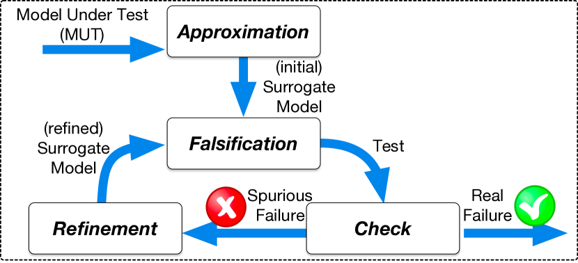
Figure 1. ARIsTEO: AppRoxImation-based TEst generatiOn.

$\bullet$ We developed ARIsTEO, an approximation-refinement testing technique, to identify requirements violations for CI-CPS models. ARIsTEO  combines falsification-based testing with surrogate models built using System Identification (SI). We have implemented ARIsTEO  as a Matlab/Simulink standalone application, relying on the existing state-of-the-art System Identification toolbox of Matlab as well as S-Taliro (Annpureddy et al., 2011), a state-of-the-art, open source falsification-based framework for Simulink models.

$\bullet$ We compared ARIsTEO and S-Taliro to assess the effectiveness and efficiency of our proposed approximation-refinement testing loop. Our experiments, performed on five publicly-available Simulink models from the literature, show that, on average, ARIsTEO  finds $23.9\%$ more requirements violations than S-Taliro and finds the violations in $31.3\%$ less time than the time S-Taliro needs to find them.

$\bullet$ We evaluated usefulness and applicability of ARIsTEO in revealing requirements violations in large and industrial CI-CPS models from the satellite domain. We analyzed three different requirements over two different versions of a CI-CPS model provided by our industrial partner. ARIsTEO successfully detected violations in each of these versions and for all the requirements, requiring four hour, on average, to find each violation. In contrast, S-Taliro was not able to find any violation on neither of the model versions and after running for four hours.

Structure. Section 2 presents our running example, formulates the problem and describes our assumptions. Section 3 describes ARIsTEO, which is then evaluated in Section 4. Section 5 presents the related work. Section 6 concludes the paper.

2. CPS Models and Falsification-Based Testing

In this section, we describe how test inputs are generated for black-box testing of CPS models. We then introduce the baseline falsification-based testing framework we use in this paper to test CPS models against their requirements.

Black-box testing of CPS models. We consider CPS models under test (MUT) specified in Simulink since it is a prevalent language used in CPS development (Liebel et al., 2018; Dajsuren et al., 2013). Our approach is not tied to the Simulink language, and can be applied to other executable languages requiring inputs and generating outputs that are signals over time (e.g., hybrid systems (Grossman et al., 1993)). Such languages are common for CPS as engineers need to describe models capturing interactions of a system with its physical environment (Alur, 2015). We use SatEx, a model of a satellite, as a running example. SatEx is a case study from our industrial partner, LuxSpace (Lux, 2019), in the satellite domain.

Let time domain $T=[0,b]$ be a non-singular bounded interval of $\mathbb{R}$. A signal is a function $f:T\rightarrow\mathbb{R}$. We indicate individual signals using lower case letters, and sets of signals using upper case letters. Let $\mathcal{M}$ be a MUT. We write $Y=\mathcal{M}(U)$ to indicate that the model $\mathcal{M}$ takes a set of signals $U=\{u_{1},u_{2}\ldots u_{m}\}$ as input and produces a set of signals $Y=\{y_{1},y_{2}\ldots y_{n}\}$ as output. Each $u_{i}$ corresponds to one model input signal, and each $y_{i}$ corresponds to one model output signal. We use the notation $u_{i}(t)$ and $y_{i}(t)$ to, respectively, indicate the values of the input signal $u_{i}$ and the output signal $y_{i}$ at time $t$. For example, the SatEx model has four input signals indicating the temperatures perceived by the Magnetometer, Gyro, Reaction wheel and Magnetorquer components, and one output signal representing the orientation (a.k.a attitude) of the satellite.

To execute a Simulink MUT $\mathcal{M}$, the simulation engine receives signal inputs defined over a time domain and computes signal outputs at successive time steps over the same time domain used for the inputs. A test input for $\mathcal{M}$ is, therefore, a set of signal functions assigned to the input signals $\{u_{1},u_{2}\ldots u_{m}\}$ of $\mathcal{M}$. To generate signal functions, we have to generate values over the time interval $T=[0,b]$. This, however, cannot be done in a purely random fashion, since input signals are expected to conform to some specific shape to ensure dynamic properties pertaining to their semantic. For examples, input signals may be constant, piecewise constant, linear, piecewise linear, sinusoidal, etc. To address this issue, we parameterize each input signal $u_{i}$ by an interpolation function, a value range $R$ and a number $n$ of control points (with $n>2$). To generate a signal function for $u_{i}$, we then randomly select $n$ control points $u_{i}(t_{1})$ to $u_{i}(t_{n})$ within $\mathbb{R}$ such that $t_{1}=0$, $t_{n}=b$ and $t_{2}$ to $t_{n-1}$ are from $T$ such that $t_{1}<t_{2}<\ldots<t_{n-1}<t_{n}$. The values of $t_{2}<t_{3}<\ldots<t_{n-1}$ can be either randomly chosen or they can be fixed with equal differences between each subsequent pairs, i.e, $(t_{i+1}-t_{i})=(t_{i}-t_{i-1})$. The interpolation function is then used to connect the $n$ control points $u_{i}(t_{1})$ to $u_{i}(t_{n})$. ARIsTEO currently supports several interpolation functions, such as piecewise constant, linear and piecewise cubic interpolation. For each input $u_{i}$ of $\mathcal{M}$, we define a triple $\langle\mathit{int}_{i},R_{i},n_{i}\rangle$, where $\mathit{int}_{i}$ is an interpolation function, $R_{i}$ is the range of signal values and $n_{i}$ is the number of control points. We refer to the set of all such triples for all inputs $u_{1}$ to $u_{m}$ of $\mathcal{M}$ as an input profile of $\mathcal{M}$ and denote it by IP. Provided with an input profile for a MUT $\mathcal{M}$, we can randomly generate test inputs for $\mathcal{M}$ as sets of signal functions for every input $u_{1}$ to $u_{m}$. For example, the input profile for SatEx provided by LuxSpace is reported in Table 1, where $[-20,50]$, $[-15,50]$, $[-20,50]$, $[-20,50]$ are real value domains.

Baseline falsification-based testing. The goal is to produce a test input $U$ that, when executed on the MUT $\mathcal{M}$, reveals a violation of some requirement of $\mathcal{M}$. Algorithm 1 represents a high-level overview of falsification-based testing. It is a black-box testing process and includes three main components: (1) a test input generation component (Generate in Algorithm 1), (2) a test objective determining whether, or not, a requirement violation is identified (TObj in Algorithm 1), and (3) a search strategy to traverse the search input space and select candidate tests (Search in Algorithm 1).

Table 1. Input Profile for the SatEx case study.

	Magnetometer	Gyro	Reaction wheel	Magnetorquer
$\mathit{int(n)}$	pchip(16)	pchip(16)	pchip(16)	pchip(16)
$R$	[-20,50]	[-15,50]	[-20,50]	[-20,50]

We describe Generate, Search and TObj. The input to the algorithm is a MUT $\mathcal{M}$ together with its input profile IP and the maximum number MAX of executions of MUT that can be performed within an allotted test budget time. Note that we choose the maximum number of executions as a loop terminating condition, but an equivalent terminating condition can be defined in term of maximum execution time.

Initial test Generation (Generate). It produces a (candidate) test input $U$ for $\mathcal{M}$ by randomly selecting control points within the ranges and applying the interpolation functions as specified in IP.

Iterative search (Search). It selects a new (candidate) test input $U$ from the search input space of $\mathcal{M}$. It uses the input profile IP to generate new test inputs. The existing candidate test input $U$ may or may not be used in the selection of the new test input. In particular, $\textsc{Search}(\mathcal{M},\texttt{IP},U)$ can be implemented using different randomized or meta-heuristic search algorithms (Nghiem et al., 2010; Matinnejad et al., 2015; Nejati et al., 2019). These algorithms can be purely explorative and generate the new test input randomly without considering the existing test input $U$ (e.g., Monte-Carlo search (Nghiem et al., 2010)), or they may be purely exploitative and generate the new test input by slightly modifying $U$ (e.g., Hill Climbing (Matinnejad et al., 2015; Nejati et al., 2019)). Alternatively, the search algorithm may combine both explorative and exploitative heuristics (e.g., Hill Climbing with random restarts (Luke, 2013)).

Algorithm 1 Baseline Falsification-based Testing.

1:function Falsification-Test($\mathcal{M}$, IP, MAX)

2:  repeat

3:   if $U$ is null then

4:    $U$ = Generate($\mathcal{M}$, IP); $\triangleright$ Generate a candidate test input

5:   else

6:    $U$ = Search($\mathcal{M}$, IP, $U$); $\triangleright$ Generate next candidate test input

7:   end if

8:   $Y=\mathcal{M}(U)$; $\triangleright$ Execute $\mathcal{M}$ for $U$

9:   if  $\textsc{TObj}(U,Y)\leq 0$ then $\triangleright$ Check if $U$ reveals a violation

10:    return $U$;

11:   end if

12:  until the number of executions of $\mathcal{M}$ reaches MAX

13:  return NULL;

14:end function

Test objective (TObj). It maps every test input $U$ and its corresponding output $Y$, i.e., $Y=\mathcal{M}(U)$, into a test objective value $\textsc{TObj}(U,Y)$ in the set $\mathbb{R}$ of real numbers. Note that computing test objective values requires simulating $\mathcal{M}$ for each candidate test input. We assume for each requirement of $\mathcal{M}$, we have a test objective TObj that satisfies the following conditions:

1. If $\textsc{TObj}(U,\mathcal{M}(U))<0$, the requirement is violated;

2. If $\textsc{TObj}(U,\mathcal{M}(U))\geq 0$, the requirement is satisfied;

3. The more positive the test objective value, the farther the system from violating its requirement; the more negative, the farther the system from satisfying its requirement.

These conditions ensure that we can infer using the value of TObj whether a test cases passes or fails, and further, TObj serves as a distance function, estimating how far a test is from violating model requirements, and hence, it can be used to guide generation of test cases. The robustness semantics of STL is an example of a semantics that satisfies those conditions (Fainekos and Pappas, 2009). An example requirement for SatEx is:

1. “the difference among the satellite attitude and the target attitude should not exceed 2 degrees”.

This requirement can be expressed in many languages including formal logics that predicate on signals, such as Signal Temporal Logics (STL) (Maler and Nickovic, 2004) and Restricted Signals First-Order Logic (RFOL) (Menghi et al., 2019). For example, this requirement can be expressed in STL as

$$\operatorname{\mathcal{G}}_{[0,\numprint{24}h]}\left(error<2\right)$$

where $error$ is the difference among the satellite attitude and the target attitude, $\operatorname{\mathcal{G}}$ is the “globally” STL temporal operator which is parametrized with the interval $[0,\numprint{24}h]$, i.e., the property $error<2$ should hold for the entire simulation time ($\numprint{24}h$).

We define a test objective TObj for this requirement as

$$\textsc{TObj}(U,M(U))=\underset{t\in[0,\numprint{24}h]}{min}\left(error(t)-2\right)$$

This is consistent with the robustness semantics of STL (Fainekos and Pappas, 2009). This value ensures the conditions $\textsc{TObj}1$, $\textsc{TObj}2$ and $\textsc{TObj}3$ since if the property is violated, i.e., there exists a time instant $t$ such that $error(t)-2<0$, a negative value is returned. In the opposite case, the property is satisfied and $\textsc{TObj}(U,\mathcal{M}(U))$ returns a non negative value. Furthermore, the more positive the test objective value, the farther the system from violating its requirement; and the more negative, the farther the system from satisfying its requirement.

In our work, we use the S-Taliro tool (Annpureddy et al., 2011) which implements the falsification-based testing shown in Algorithm 2. S-Taliro is a well-developed, open source research tool for falsification based-testing and has been recently classified as ready for industrial deployment (Kapinski et al., 2016). It has been applied to several realistic and industrial systems (Tuncali et al., 2018) and based on a recent survey on the topic (Kapinski et al., 2016) is the most mature tool for falsification of CPSs. Further, S-Taliro supports a range of standard search algorithms such as Simulated Annealing, Monte Carlo (Nghiem et al., 2010), and gradient descent methods (Abbas et al., 2014).

Test objectives can be defined manually. Alternatively, assuming that the requirements are specified in logic languages, test objectives satisfying the three conditions we described earlier can be generated automatically. In particular, we have identified two existing tools that generate quantitative test objectives from requirements encoded in logic-based languages: Taliro (Fainekos and Pappas, 2008) and Socrates (Menghi et al., 2019). In this paper, we use Taliro since it is integrated into S-Taliro. To do so, we specified our requirements into Signal Temporal logic (STL) (Maler and Nickovic, 2004) and used Taliro to automatically convert them into quantitative test objectives capturing degrees of satisfaction and refutation conforming to our conditions $\textsc{TObj}1$-$\textsc{TObj}3$ on test objectives.

3. ARIsTEO

Algorithm 2 shows the approximation-refinement loop of ARIsTEO. The algorithm relies on the following inputs: a CI-CPS model $\mathcal{M}$ (i.e., the model under test—MUT), the input profile IP of MUT, and the maximum number of iterations MAX_REF that can be executed by ARIsTEO. In the first iteration, an initial surrogate model $\hat{\mathcal{M}}$ is computed such that it approximates the MUT behavior (Line 4). Note that $\hat{\mathcal{M}}$ is built such that it has the same input profile as $\mathcal{M}$, i.e., $\hat{\mathcal{M}}$ and $\mathcal{M}$ have exactly the same inputs and outputs. At every iteration, the algorithm applies falsification-based testing to the surrogate model $\hat{\mathcal{M}}$ in order to find a test input $U$ violating the requirement captured by the test objective TObj (Line 8). The number MAX of iterations of falsification-based testing for $\hat{\mathcal{M}}$ is an internal parameter of ARIsTEO, and in general, can be set to a high value since executing $\hat{\mathcal{M}}$ is not expensive. Once $U$ is found, the algorithm checks whether $U$ leads to a violation when it is checked on the MUT (Line 9). Recall from Section 2 that test objectives TObj are defined such that a negative value indicates a requirement violation. If so, $U$ is returned as a failure-revealing test for $\mathcal{M}$ (Line 10). Otherwise, $U$ is spurious and in the next iteration it is used to refine the surrogate model $\hat{\mathcal{M}}$ (Line 6). If no failure-revealing test for $\mathcal{M}$ is found after MAX_REF iterations the algorithm stops and a null value is returned.

Algorithm 2 The ARIsTEO Main Loop.

1:function ARIsTEO($\mathcal{M},\texttt{IP},\texttt{MAX\_REF}$)

2:  repeat

3:   if $\hat{\mathcal{M}}$ is null then

4:    $\hat{\mathcal{M}}$=Approximate($\mathcal{M}$); $\triangleright$ Generate a surrogate model

5:   else

6:    $\hat{\mathcal{M}}$=Refine($\hat{\mathcal{M}}$,$U$,$\mathcal{M}$); $\triangleright$ Refine the surrogate model

7:   end if

8:   $U$=Falsification-Test($\hat{\mathcal{M}},\texttt{IP},\texttt{MAX}$);

9:   if TObj($U$, $\mathcal{M}$($U$)) $\leq 0$ then $\triangleright$ Test $U$ finds a real violation

10:    return $U$;

11:   end if

12:  until the number of executions of $\mathcal{M}$ reaches MAX_REF

13:  return NULL;

14:end function

The falsification-based testing procedure is described in Section 2 (Algorithm 1). In Section 3.1, we describe the Approximate method (line 4), and in Section 3.2, we describe the Refine method (line 6).

Table 2. Model structure and parameter choices for developing surrogate models.

Linear	Model Structure	Equation	Model Type
	arx($na,nb,nk$)	$y(t)=a_{1}\cdot y(t-1)+\ldots+a_{na}\cdot y(t-na)+b_{1}\cdot u(t-nk)+\ldots+b_{nb}\cdot u(t-nb-nk+1)+e(t)$	Discrete
	Description
	The output $y$ depends on previous input values, i.e., $u(t-nk),$…$,u(t-nb-nk+1)$, and on values assumed by the output $y$ in previous steps, i.e., $y(t-1),$…$,y(t-na)$. $na$ and $nb$ are the number of past output and input values to be used in predicting the next output. $nk$ is the delay (number of samples) from the input to the output.
	Model Structure	Equation	Model Type
	armax($na,nb,nk,nc$)	$y(t)=a_{1}\cdot y(t-1)+\ldots+a_{na}\cdot y(t-na)+b_{1}\cdot u(t-nk)+\ldots+b_{nb}\cdot u(t-nb-nk+1)+c_{1}\cdot e(t-1)+\ldots+c_{nc}\cdot e(t-nc)+e(t)$	Discrete
	Description
	Extends the arx model by considering how the values $e(t-1),$…$,e(t-nc)$ of the noise $e$ at time $t$, $t-1$, $\ldots$, $t-nc$ influence the value $y(t)$ of the output $y$.
	Model Structure	Equation	Model Type
	bj($nb,nc,nf,nd,nk$)	$y(t)=\frac{B(z)}{F(z)}\cdot u(t)+\frac{C(z)}{D(z)}\cdot e(t)$	Discrete
	Description
	Box-Jenkins models allow a more general noise description than armax models. The output $y$ depends on a finite number of previous input $u$ and output $y$ values. The values $n_{b}$, $n_{c}$, $n_{d}$, $n_{f}$, $n_{k}$ indicate the parameters of the matrix $B$, $C$, $D$, $F$ and the value of the input delay.
	Model Structure	Equation	Model Type
	tf($np,nz$)	$y(t)=\frac{b_{0}+b_{1}\cdot s+b_{2}\cdot s^{2}+\ldots+b_{n}\cdot s^{n_{z}}}{1+f_{1}\cdot s+f_{2}\cdot s^{2}+\ldots+f_{m}\cdot s^{n_{p}}}\cdot u(t)+e(t)$	Continuous
	Description
	Represents a transfer function model. The values $n_{p}$, $n_{z}$ indicate the number of poles and zeros of the transfer function.
	Model Structure	Equation	Model Type
	ss($n$)	$x(0)=x0$ $\dot{x}(t)=Fx(t)+Gu(t)+Kw(t)$ $y(t)=Hx(t)+Du(t)+w(t)$	Continuous
	Description
	Uses state variables to describe a system by a set of first-order differential or difference equations. $n$ is an integer indicating the size of the matrix $F$, $G$, $K$, $H$ and $D$.
Non Linear	Model Structure	Equation	Model Type
	nlarx($f,na,nb,nk$)	$y(t)=f(y(t-1),...,y(t-na),u(t-nk),...,u(t-nk-nb+1))$	Discrete
	Description
	Uses a non linear function $f$ to describe the input/output relation. Wavelet, sigmoid networks or neural networks in the Deep Learning Matlab Toolbox (dee, 2019) can be used to compute the function $f$. $na$ and $nb$ are the number of past output and input values used to predict the next output value. $nk$ is the delay from the input to the output.
	Model Structure	Equation	Model Type
	hw($f,h,na,nb,nk$)	$w(t)=f(u(t))$ $x(t)=(B(z)/F(z))\cdot w(t)$ $y(t)=h(x(t))$	Continuous
	Description
	Hammerstein-Wiener models describe dynamic systems two nonlinear blocks in series with a linear block. Specifically, $f$ and $h$ are non linear functions, $B(z)$, $F(z)$, $na$, $nb$, $nk$ are defined as for bj models. Different nonlinearity estimators can be used to learn $f$ and $h$ similarly to the nlarx case.

3.1. Approximation

Given an MUT $\mathcal{M}$, the goal of the approximation is to produce a surrogate model $\hat{\mathcal{M}}$ such that: (C1) $\mathcal{M}$and $\hat{\mathcal{M}}$ have the same interface, i.e., the same inputs and outputs; (C2) provided with the same input values, they generate similar output values; and (C3) $\hat{\mathcal{M}}$is less expensive to execute than $\mathcal{M}$ .

We rely on System Identification (SI) techniques to produce surrogate models (Söderström and Stoica, 1989) since their purpose is to automatically build mathematical models of dynamical systems from data when it is difficult to build the models analytically, or when engineers want to build models from data obtained based on measurements of the actual hardware. Note that the more complex SI structures (i.e., non-linear nlarx and hw) rely on machine learning and neural network algorithms (Ljung, 2008).

To build $\hat{\mathcal{M}}$ using SI, we need some input and output data from the MUT $\mathcal{M}$. Since $\mathcal{M}$ is expensive to execute, to build the initial surrogate model $\hat{\mathcal{M}}$ (line 6), we run $\mathcal{M}$ for one input $U$ only. Note that an input $U$ of $\mathcal{M}$ is a set $\{u_{1},\ldots,u_{m}\}$ of signal functions over $T=[0,b]$. So, each $u_{i}$ is a sequence $u_{i}(0),u_{i}(\delta),u_{i}(2\cdot\delta)\ldots u_{i}(l\cdot\delta)$ where $b=l\cdot\delta$ and $\delta$ is the sampling rate applied to the time domain $[0,b]$. Similarly, the output $Y=\mathcal{M}(U)$ is a set $\{y_{1},\ldots,y_{n}\}$ of signal functions where each $y_{j}$ is a sequence $y_{j}(0),y_{j}(\delta),y_{j}(2\cdot\delta)\ldots y_{j}(l\cdot\delta)$ obtained based on the same sampling rate and the same time domain as those used for the input. We refer to the data used to build $\hat{\mathcal{M}}$ as traning data and denote it by $\mathcal{D}$. Specifically, $\mathcal{D}=\langle U,Y\rangle$. For CI-CPS, the size $l$ of $\mathcal{D}$ tends to be large since we typically execute such models for a long time duration (large $b$) and use a small sampling rate (small $\delta$) for them. For example, we typically run SatEx for $b=\numprint{86400}$s ($24$h) and use the sampling rate $\delta=0.0312$s. Hence, a single execution of SatEx generates a training data set $\mathcal{D}$ with size $l=\numprint{2769200}$. Such training data size is sufficient for SI to build reasonably accurate surrogate models.

We use the System Identification Toolbox (Ljung, 2008) of Matlab to generate surrogate models. In order to effectively use SI, we need to anticipate the expected structure and parameters of surrogate models, a.k.a configuration. Table 2 shows some standard model structures and parameters supported by SI. Specifically, selecting the model structure is about deciding which mathematical equation among those shown in Table 2 is more likely to fit to our training data and is better able to capture the dynamics of the model $\mathcal{M}$. As shown in Table 2, equations specifying the model structure have some parameters that need to be specified so that we can apply SI techniques. For example, for arx($na,nb,nk$), the values of the parameters $na$, $nb$ and $nk$ are the model parameters.

Table 2 provides a short description for each model structure. We note that some of the equations in the table are simplified and refer to the case in which the MUT has a single input signal and a single output signal. The equations, however, can be generalized to models with multiple input and output signals. Briefly, model structures can be linear or non-linear in terms of the relation between the inputs and outputs, or they can be continuous and discrete in terms of their underlying training data. Specifically, the training data generated from MUT can be either discrete (i.e., sampled at a fixed rate) or continuous (i.e., sampled at a variable rate). Provided with discrete training data, we can select either continuous or discrete model structures, while for continuous training data, we can select continuous model structures only. As discussed earlier, our training data $\mathcal{D}$ is discrete since it is sampled at the fix sampling rate of $\delta$. Hence, we can choose both types of model structures to generate surrogate models. In our work we support training data sampled at a fixed sampling rate to build and refine the surrogate models. Data sampled at a variable time rate can be then handled by exploiting the resampling procedure of Matlab (Res, 2019).

The users of ARIsTEO need to choose upfront the configuration to be used by the SI, i.e., the model structure and the values of its parameters. This choice depends on domain specific knowledge that the engineers possess for the model under analysis. The values of the parameters selected by the user should be chosen such that the resulting surrogate model (i) has the same interface as the MUT to ensure C1 and (ii) has a simpler structure than the MUT to ensure C3. The System Identification Toolbox provides some generic guidance for selecting the parameters ensuring these two criteria (mod, 2019). In this work we performed an empirical evaluation over a set of benchmark models to determine the configuration to be used in our experiments (Section 4.1).

Once a configuration is selected, SI uses the training data to learn values for the coefficients of the equation from Table 2 that corresponds to the selected structure and paramters. For example, after selecting arx($na,nb,nk$) and assigning values to $na$, $nb$ and $nk$, SI generates a surrogate model by learning values for the coefficients: $a_{1},\ldots a_{na}$ and $b_{1},\ldots b_{nb}$.

Similar to standard machine learning algorithms, SI’s objective is to compute the model coefficients by minimizing the difference (error) between the outputs of $\mathcal{M}$ and $\hat{\mathcal{M}}$ for the training data (Söderström and Stoica, 1989). SI uses different standard notions of errors depending on the model structure selected. In our work, we compute the Mean Squared Error (MSE) (Söderström and Stoica, 1989) between the outputs of $\mathcal{M}$ and $\hat{\mathcal{M}}$.

SI learns a surrogate model $\hat{\mathcal{M}}$ by minimizing MSE over the training data $\mathcal{D}$ and hence, ensuring C2. The learning algorithm selected by SI depends on the chosen model structure, on the purpose of the identification process, i.e., whether the identified model will be used for prediction or simulation, and on whether the system is continuous or discrete.

3.2. Refinement

The refinement step rebuilds the surrogate model $\hat{\mathcal{M}}$ when the test input $U$ obtained by falsification-based testing of the surrogate model is spurious for MUT (i.e., it does not reveal any failure according to the test objective). Note that $\hat{\mathcal{M}}$ may not be sufficiently accurate to predict the behavior of the MUT. Hence, it is likely that we need to improve its accuracy and we do so by reusing the data obtained when checking a candidate test input $U$ on MUT (line 9 of Algorithm 2).

Let $U=\{u_{1},\ldots,u_{m}\}$ and $Y=\{y_{1},\ldots,y_{n}\}$ be the spurious test inputs and its output, respectively. Similar to the data used to build the initial $\hat{\mathcal{M}}$ by the approximate step (line 9 of Algorithm 2), the data $\mathcal{D}^{\prime}=\langle U,Y\rangle$ used to rebuild $\hat{\mathcal{M}}$ is also discretized based on the same sampling rate $\delta$. To refine the surrogate model, we do not change the considered configuration, but we combine the new $\mathcal{D}^{\prime}$ and existing training data $\mathcal{D}$, and refine $\hat{\mathcal{M}}$ using these data.

Alternative policies can be chosen to refine the surrogate model. For example, the refinement activity may also change the configuration of ARIsTEO. This is a rather drastic change in the surrogate model. When engineers have a clear understanding of the underlying model, they may be able to define a systematic methodology on how to move from less complex structures (e.g., linear) to more complex ones (e.g., non-linear). Without proper domain knowledge, such modification may be too disruptive. In this paper, our refinement strategy is focused on incrementing the training data and rebuilding the surrogate model without changing the configuration.

4. Evaluation

In this section, we empirically evaluate ARIsTEO by answering the following research questions:

$\bullet$ Configuration - RQ1. Which are the optimal (most effective and efficient) SI configurations for ARIsTEO? Which of the optimal configurations can be used in the rest of our experiments? We investigate the performance of ARIsTEO  for different SI configurations (model structures and parameters listed in Table 2) to identify the optimal ones, i.e., those that offer the best trade-offs between effectiveness (revealing the most requirements violations) and efficiency (revealing the violations in less time). We then select one configuration among the optimal ones and use that configuration for the rest of our experiments.

$\bullet$ Effectiveness - RQ2. How effective is ARIsTEO in generating tests that reveal requirements violations? We use ARIsTEO with the optimal configuration identified in RQ1 and evaluate its effectiveness (i.e., its ability in detecting requirements violations) by comparing it with falsification-based testing without surrogate models. We use S-Taliro discussed in Section 2 for the baseline of comparison.

$\bullet$ Efficiency - RQ3. How efficient is ARIsTEO  in generating tests revealing requirements violations? We use ARIsTEO with the optimal configuration identified in RQ1 and evaluate its efficiency (i.e., the time it takes to find violations) by comparing it with falsification-based testing without surrogate models (i.e., S-Taliro).

A key challenge regarding the empirical evaluation of ARIsTEO  is that, both ARIsTEO  and S-Taliro rely on randomized algorithms. Hence, we have to repeat our experiments numerous times for different models and requirements so that the results can analysed in a sound and systematic way using statistical tests (Arcuri and Briand, 2014). This is necessary to answer RQ1-RQ3 that involve selecting an optimal configuration and comparing ARIsTEO  with the baseline S-Taliro. Performing these experiments on CI-CPS models is, however, extremely expensive, to the point that the experiments become infeasible. A ballpark figure for the execution time of the experiments required to answer RQ1-RQ3 is around 50 years if the experiments are performed on our CI-CPS model case study (SatEx). Therefore, instead of using CI-CPS models, we use non-CI-CPS models to address RQ1-RQ3. The implications of this decision on the results are assessed and mitigated in Sections 4.1 and 4.2 where we discuss these three research questions in detail. In addition, to be able to still assess the performance of ARIsTEO on CI-CPS models, we consider an additional research question described below:

Table 3. Non-CI-CPS subject models. ID: model identifier; #B: number of blocks of the Simulink model; #I: number of inputs of the Simulink model; int(n): input interpolation functions and number of control points; R: input ranges; and T: time domain.

ID	#B	#I	int(n)	R	T
RHB(1)	28	1	pchip(4)	$[-2,5]^{*}$	24
RHB(2)	31	2	pchip(4),const(1)	$[-2,5]$, $[0.8,1.2]$	24
AT	63	1	pconst(7)	$[0,100]$	30
AFC	302	2	const(1),pulse(10)	$[900,1100]$, $[0,61.1]$	50
IGC	70	10	const(1),const(1), const(1),const(1), const(1),const(1), const(1),const(1), const(1),const(1)	$[40,40]$,$[30,30]$, $[200,200]$,$[40,40]$, $[150,250]$,$[0,80]$, $[20,50]$,$[100,300]$, $[20,70]$,$[-0.3,0.3]$	400

$\bullet$ Usefulness - RQ4. How applicable and useful is ARIsTEO in generating tests revealing requirements violations for industrial CI-CPS models? We apply ARIsTEO  with the optimal configuration identified in RQ1 to our CI-CPS model case study from the satellite industry (SatEx) and evaluate its effectiveness and efficiency. The focus here is to obtain representative results in terms of effectiveness and efficiency based on an industry CI-CPS model. Note that we still apply S-Taliro to SatEx to be able to compare it with ARIsTEO for an industry CI-CPS model. This comparison, however, is not meant to be subject to statistical analysis due to the large execution time of SatEx, and is only meant to complement RQ3 with a fully realistic though extremely time consuming study.

The subject models. We used five publicly available non-CI-CPS models (i.e., RHB(1), RHB(2), AT, AFC, IGC) that have been previously used in the literature on falsification-based testing of CPS models (Fehnker and Ivancic, 2004; Dang et al., 2004; Zhao et al., 2003; Jin et al., 2014; Sankaranarayanan and Fainekos, 2012b; Ernst et al., 2019). The models represent realistic and representative models of CPS systems from different domains. RHB(1) and RHB(2) (Fehnker and Ivancic, 2004) are from the IoT and smart home domain. AFC (Jin et al., 2014) is from the automotive domain and has been originally developed by Toyota. AT (Zhao et al., 2003) is another model from the automotive domain. IGC (Sankaranarayanan and Fainekos, 2012b) is from the health care domain. AT and AFC have also been recently considered as a part of the reference benchmarks in the ARCH competition (Ernst et al., 2019) – an international competition among verification and testing tools for continuous and hybrid systems (cps, 2019). In Table 3, we report the number of blocks and inputs, the input profiles, input ranges and simulation times for the five non-CI-CPS models. These models have been manually developed and may violate their requirements due to human error. Some of the violations have been identified by the existing testing tools and are reported in the literature (Fehnker and Ivancic, 2004; Jin et al., 2014; Zhao et al., 2003; Sankaranarayanan and Fainekos, 2012b; Ernst et al., 2019). As for the CI-CPS model to address RQ4, we use the SatEx case study that we introduced as a running example in Sections 2 and 3. SatEx contains $2192$ blocks and has to be simulated for $24$h for each test case to sufficiently exercise the system dynamics and interactions with the environment. Like the models in Table 3, SatEx is manually developed by engineers and is likely to be faulty. Its inputs and input profiles are shown in Table 1.

Implementation and Data Availability. We implemented ARIsTEO as a Matlab application and as an add-on of S-Taliro. Our (sanitized) models, data and tool are available online (app, 2019) and are also submitted alongside the paper.

4.1. RQ1 - Configuration

Recall that ARIsTEO requires to be provided with a configuration to build surrogate models. The universe of the possible configurations is infinite as the model structures in Table 2 can be parametrized in an infinite number of ways by associating different values to their parameters. RQ1 identifies the optimal configurations that yield the best tradeoff between effectiveness and efficiency for ARIsTEO among a reasonably large set of alternative representative configurations. It then selects one among the optimal configurations.

We do not evaluate configurations by measuring their prediction accuracy (i.e., by measuring their prediction error when applied to a set of test data as is common practice in assessing prediction models in the machine learning area (Bishop, 2006)) because our focus is not to have the most accurate configuration but the one that is able to have the most effective impact on ARIsTEO’s approximation-refinement loop by quickly finding requirements violations. However, it is likely that there exists a relationship between the two.

Experiment design. We consider five different configurations obtained by five different sets of parameter values for each model structure in Table 2. We denote the five configurations related to each model structure $S$ by $S_{1}$ to $S_{5}$. For example, the configurations related to the model structure ss are denoted by ss₁ to ss₅. The specific parameter value sets for the 35 configurations based on the seven model structures in Table 2 are available online (app, 2019).

To answer RQ1, we apply ARIsTEO  to the five non-CI-CPS models using each configuration among the 35 possible ones. That is, we execute ARIsTEO  for 175 times. We further rerun each application of ARIsTEO  for 100 times to account for the randomness in both falsification-based testing and the approximation-refinement loop of ARIsTEO (Ben Abdessalem et al., 2018). We set the value of MAX_REF, i.e, the number of iterations of the ARIsTEO’s main loop, to 10 (see Algorithm 2) and the value of MAX, i.e, the number times each iteration of ARIsTEO executes falsification-based testing (see Algorithm 1), to $100$ for RHB(1), RHB(2) and AFC, and to $1000$ for AT and IGC. These values were used in the original experiments that apply falsification-based testing to these models (ben, 2019). Running all the 17,500 experiments required 4 315 567 hours ($\approx$ 99 days).

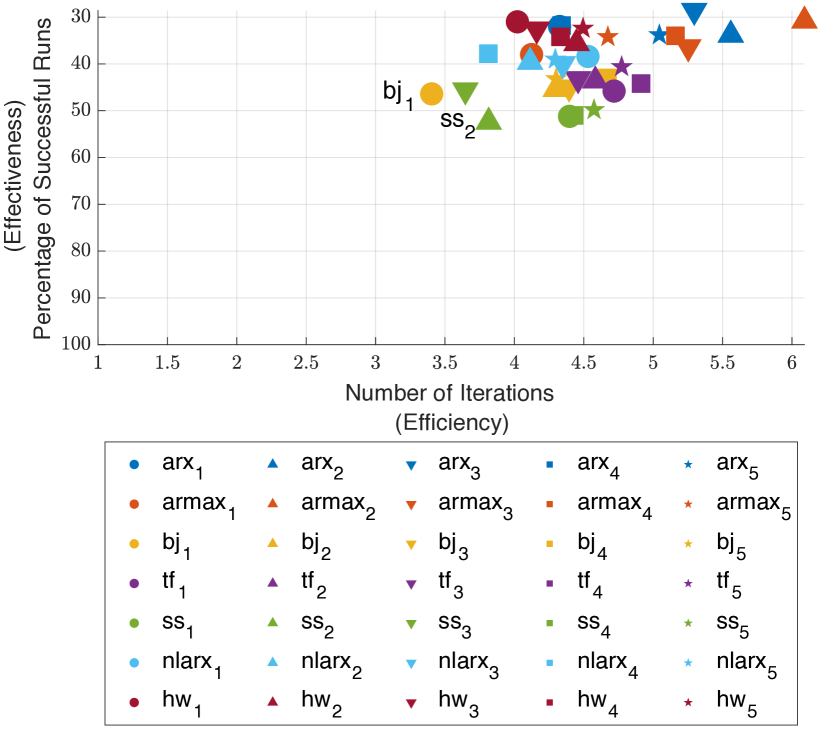
Figure 2. Effectiveness and efficiency of different configurations across our non-CI-CPS subject models.

Due the sheer size of the experiments required to answer RQ1, we used our non-CI-CPS subject models. While these models are smaller than typical CI-CPS models, the complexity of their structure (how Simulink blocks are used and connected) is similar to the one of SatEx. Specifically, the structural complexity index (Plaska et al., 2009; Olszewska, 2011), which provides an estimation of the complexity of the structure of a Simulink model, is $1.8$, $1.6$, $1.2$, $1.1$, $2.1$ for the RHB(1), RHB(2), AT, AFC and IGC benchmarks, respectively, and $1.5$ for the SatEx case study. We conjecture that given these similarities, the efficiency and effectiveness comparisons of the configurations performed on non-CI-CPS models would likely remain the same should the comparisons be performed on CI-CPS models. However, due to computational time restrictions, we are not able to check this conjecture. Finally, we note that even if we select a sub-optimal configuration, it will be a disadvantage for ARIsTEO. So, the results for RQ2-RQ4 are likely to improve if we find a way to identify a better configuration for ARIsTEO using CI-CPS models.

Results. The scatter plot in Figure 2 shows the results of our experiments. The x-axis indicates our efficiency metric which is defined as the number of iterations that ARIsTEO requires to reveal a requirement violation in a model for a given configuration. As described in the experiment design, the maximum number of iterations is 10. Given a configuration for ARIsTEO, the fewer iterations required to reveal a violation, the more efficient that configuration is. The y-axis indicates our effectiveness metric which is defined as the number of ARIsTEO  runs (out of 100) that can reveal a violation in a model. For effectiveness we are interested to know how often we are able to reveal a requirement violation. The higher the number of runs detecting violations, the more effective that configuration is. The ideal configuration is the one that finds requirements violations in 100% of the runs in just one iteration as indicated by the origin of the plot in Figure 2 with coordinates $(1,100)$.

For each configuration, there is one point in the plot in Figure 2 whose coordinates, respectively, indicate the average efficiency and effectiveness of that configuration for the non-CI-CPS subject models. As shown in the figure, bj₁ and ss₂ are on the Pareto frontier (par, 2019) and dominate other configurations in terms of efficiency and effectiveness. That is, any configuration other than bj₁ and ss₂ is strictly dominated in terms of both efficiency and effectiveness by either bj₁ or ss₂. But bj₁ does not dominate ss₂, and neither does ss₂. Specifically, bj₁ is more efficient but less effective than ss₂, and ss₂ is less efficient but more effective than bj₁. For our experiments, we select bj₁ as the optimal configuration since efficiency is paramount when dealing with CI-CPS models. In terms of effectiveness, bj₁ is only slightly less effective than ss₂ (46.4% versus 52.4%).

The answer to RQ1 is that, among all the 35 configurations we compared, the bj₁ and the ss₂ configurations are the optimal configurations offering the best trade-off between efficiency (i.e., time required to reveal requirements violations) and effectiveness (i.e., number of violations revealed) for ARIsTEO. We select bj₁ as we prioritize efficiency.

4.2. RQ2 and RQ3 - Effectiveness and Efficiency

For RQ2 and RQ3, we compare ARIsTEO (Algorithm 2) with S-Taliro (Algorithm 1). As discussed earlier, due to the large size of the experiments, we use non-CI-CPS models, but we want to obtain results that are representative for the CI-CPS case. For such comparisons, we need to execute both tools for an equivalent amount of time and then compare their effectiveness and efficiency. This is a non trivial problem, because

• That equivalent amount of time cannot simply translate into identical execution times. Non-CI-CPS models, by definition, are very quick to execute. Hence, the benefits of performing the falsification on the surrogate model, as done by ARIsTEO, would not be visible if we compared the two tools based on the execution times of non-CI-CPS models. Therefore, comparisons would be in favour of S-Taliro if we fix the execution times of the two tools for non-CI-CPS models.

• Neither can we can run the two tools for the same number of iterations, as commonly done in this domain (Ernst et al., 2019), because one iteration of ARIsTEO takes more time than one iteration of S-Taliro. Recall that ARIsTEO, in addition to performing falsification, builds and refines surrogate models in each iteration. Thus, by fixing the number of iterations for the two tools, comparisons would be in favour of ARIsTEO.

To answer RQ2 and RQ3 without favouring neither of the tools, we propose the following:

Suppose that we could perform RQ2 and RQ3 on a CI-CPS model, and that we execute ARIsTEO and S-Taliro on this model for the same time limit $TL$. Let $IA$ and $IB$ be the number of iterations of ARIsTEO and S-Taliro within $TL$, respectively. Recall that one iteration of ARIsTEO  typically takes more time than one iteration of the baseline ($IA<IB$). If we know the values of $IA$ and $IB$, we can execute ARIsTEO for $IA$ times and S-Taliro for $IB$ times on non-CI-CPS models and use the results to compare the tools as if they were executing on CI-CPS models.

To run our experiment, we need to know the relation between $IA$ and $IB$. We approximate this relation empirically using our SatEx  CI-CPS model. We execute ARIsTEO for $10$ iterations and we set the number of falsification iterations in each iteration of ARIsTEO  to $100$ as suggested by the literature on CPS falsification testing (Annpureddy et al., 2011; ben, 2019) (i.e., MAX_REF = 10 and MAX = $100$ in Algorithm 2). We repeated these runs of ARIsTEO  for five times. The first iteration of ARIsTEO  took, on average, 16 902s, and the subsequent iterations of ARIsTEO  took, on average, 9 865s. Note that the first iteration of ARIsTEO  is always more expensive than the subsequent iterations since ARIsTEO builds surrogate models in the first iteration. Similarly, we executed S-Taliro for 10 iterations on SatEx, and repeated this run for five times. Each iteration of S-Taliro took, on average, 8 336s on SatEx. This preliminary experiment took approximately 20 days. We then solve the two equations below to approximate the relation between $IA$ and $IB$:

(1) $$TL=\numprint{9865}\times(IA-1)+\numprint{16902}$$

(2) $$TL=\numprint{8336}\times IB$$

The above yields $IB=1.2\times IA+0.8$. Though we obtained this relation between $IA$ and $IB$ based on one CI-CPS case study, SatEx  is a large and industrial system representative of the CPS domain. Further, for CI-CPS models that are more compute-intensive than SatEx, executing the models takes even more time compared to the approximation and refinement time, and hence, the relation above could be further improved in favour of ARIsTEO.

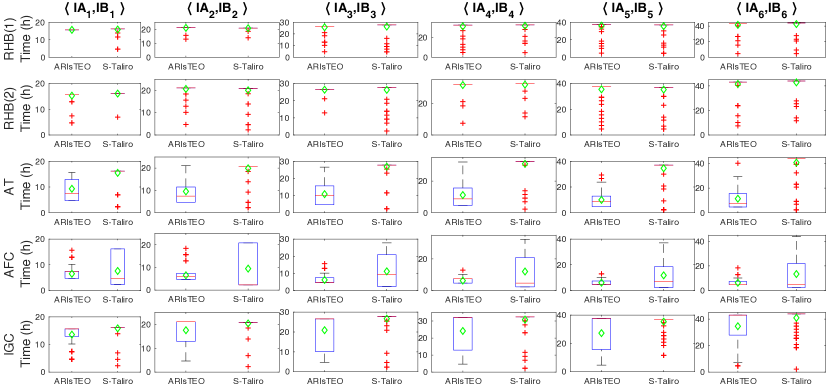
Figure 3. Comparing the efficiency of ARIsTEO and S-Taliro. The box plots show the execution time (computed using equations 1 and 2) of ARIsTEO and S-Taliro (in hours) for our non-CI-CPS subject models (labels on the left of the figure) and over different iterations (labels on the top of the figure). Diamonds depict the average.

Table 4. The effectiveness results. Percentages of cases in which ARIsTEO (IA_i labelled columns) and S-Taliro (IB_i labelled columns) were able to detect requirements violations for different iteration pairs (IA_i and IB_i) and benchmarks.

	IA1	IB1	IA2	IB2	IA3	IB3	IA4	IB4	IA5	IB5	IA6	IB6
RHB(1)	0%	5%	2%	2%	8%	8%	7%	7%	11%	6%	9%	8%
RHB(2)	5%	2%	6%	8%	4%	9%	5%	10%	13%	10%	7%	10%
AT	85%	7%	92%	7%	93%	7%	99%	4%	100%	8%	100%	13%
AFC	100%	77%	100%	73%	100%	88%	100%	86%	100%	92%	100%	95%
IGC	33%	4%	31%	6%	34%	9%	37%	15%	40%	18%	13%	21%

Experiment design. To answer RQ2 and RQ3, we applied ARIsTEO with the configuration identified by RQ1 (bj₁) and S-Taliro to the five non-CI-CPS models in Table 3. We executed ARIsTEO and S-Taliro for the following pairs of iterations: $\langle IA_{1}=5,IB_{1}=7\rangle$, $\langle IA_{2}=7,IB_{2}=9\rangle$, $\langle IA_{3}=9,IB_{3}=12\rangle$, $\langle IA_{4}=11,IB_{4}=14\rangle$, $\langle IA_{5}=13,IB_{5}=16\rangle$, and $\langle IA_{6}=15,IB_{6}=19\rangle$. Note that every pair approximately satisfies $IB_{i}=1.2\times IA_{i}+0.8$. We repeated each run 100 times to account for their randomness. For RQ2, we compute the effectiveness metric as in RQ1: the number of runs revealing requirements violations (out of 100) for each tool. For RQ3, we assess efficiency by computing the efficiency metric as in RQ1: the number of iterations that each tool requires to reveal a requirement violation. However, as discussed above, the number of iterations of ARIsTEO and S-Taliro are not comparable. Hence, for RQ3, we report efficiency in terms of the estimated time that each tool needs to perform those iterations on CI-CPS models computed using equations 1 and 2.

Results-RQ2. Table 4 shows the effectiveness values for ARIsTEO  and S-Taliro for the five iteration pairs discussed in the experiment design. For the AT, AFC and IGC models, the average effectiveness of ARIsTEO  is significantly higher than that of S-Taliro ($75.4\%$ versus $35.0\%$ on average across benchmarks), while for RHB(1) and RHB(2), ARIsTEO  and S-Taliro reveal almost the same number of violations ($6.4\%$ versus $7.0\%$ on average across benchmarks). The former difference in proportion is statistically significant as confirmed by a two-sample z-test (McDonald, 2009) with the level of significance ($\alpha$) set to 0.05.

RHB(1) and RHB(2) have more outputs than the other benchmarks and they have shorter simulation times (see Table 3). This is an increased challenge for building accurate surrogate models. In practice, CI-CPS models can have a large number of outputs but they usually involve long simulation times.

The answer to RQ2 is that ARIsTEO is significantly more effective than S-Taliro for three benchmark models while, for the other two models, they reveal almost the same number of violations. On average, over the five models, ARIsTEO  detects $23.9\%$ more requirements violations than S-Taliro (min=-8%, max=95%).

Results-RQ3. The execution times (computed using equations 1 and 2) of ARIsTEO and S-Taliro for our non-CI-CPS subject models and the iteration pairs $\langle IA_{i},IB_{i}\rangle$ are shown in Figure 3. The box plots in the same row are related to the same benchmark model, while the box plots in the same column are related to the same iteration pair. Recall that we described the iteration pairs $\langle IA_{i},IB_{i}\rangle$ considered for our experiments earlier in the experiment design subsection. As expected, the average execution times of the two tools increases with their number of iterations.

To statistically compare the results, we used the Wilcoxon rank sum test (McDonald, 2009) with the level of significance ($\alpha$) set to $0.05$. The results show that ARIsTEO  is significantly more efficient than S-Taliro for the AT and IGC models (Figure 3 – rows 3,5). The efficiency improvement that ARIsTEO  brings about over S-Taliro for AT and IGC across different iterations ranges from $14.4\%$ ($2.2$h) to $73.1\%$ ($31.2$h). Note that, for AT and IGC, ARIsTEO is significantly more effective than S-Taliro (see Table 4). This shows that, many runs of ARIsTEO for AT and IGC can reveal a requirement violation and stop before reaching the maximum ten iterations, hence yielding better efficiency results of ARIsTEO  compared to the other model.

For the RHB(1) and RHB(2) models (Figure 3 – rows 1,2), ARIsTEO and S-Taliro yield comparable efficiency results. The effectiveness results in Table 4 confirm that, for RHB(1) and RHB(2), both ARIsTEO and S-Taliro have to execute for ten iterations most of the times as they cannot reveal violations (low effectiveness). Hence, the efficiency results are worse for RHB(1) and RHB(2) than for the other models. Further, as we run the tools for more iterations, the efficiency results slightly increases as indicated by the increase in the number of outliers. For the AFC model (Figure 3 – row 4), ARIsTEO is slightly more efficient than S-Taliro. For AFC, S-Taliro is relatively effective in finding violations, and hence, is efficient. But, its average execution time is slightly worse than that of ARIsTEO. Comparing the interquartile ranges of the box plots shows that ARIsTEO is generally more efficient that S-Taliro. However, a Wilcoxon test does not reject the null hypothesis (p-value = 0.06).

The average execution time of ARIsTEO and S-Taliro across the different models is, respectively, approximately $19$h and $25$h. Though there is significant variation across the different models, ARIsTEO is, on average, $31.3\%$ more efficient than S-Taliro.

The answer to RQ3 is that ARIsTEO is on average $31.3\%$ (min=$-1.6\%$, max=$85.2\%$) more efficient than S-Taliro.

4.3. RQ4 - Practical Usefulness

We assess the usefulness of ARIsTEO  in revealing requirements violations of a representative industrial CI-CPS model.

Experiment design. We received three different requirements from our industry partner (Lux, 2019). One is the SatReq requirement presented in Section 2, and the two others (SatReq1 and SatReq2) are strengthened versions of SatReq that, if violated, indicate increasingly critical violations. We also received the input profile IP (Section 2) and a more restricted input profile IP^′, representing realistic input subranges associated with more critical violations. For each combination of the requirement (SatReq, SatReq1 and SatReq2) and the input profiles IP and IP^′, we checked whether ARIsTEO was able to detect any requirement violation, and further, we recorded the time needed by ARIsTEO  to detect a violation. In addition, for the two most critical requirements (SatReq1 and SatReq2) and the input profiles IP and IP^′, we checked whether S-Taliro is able to detect any violation within the time limit required by ARIsTEO to successfully reveal violations for SatReq1 and SatReq2. Running this experiment took approximately four days and both tools were run twice for each requirement and input profile combination.

Results. ARIsTEO found a violation for every requirement and input profile combination in our study in just one iteration, requiring approximately four hours of execution time. Given that simulating the model under test takes approximately an hour and a half, detecting errors in four hours is highly efficient as it corresponds to roughly two model simulations. In comparison, S-Taliro failed to find any violations for SatReq1 and SatReq2 after running the tool for four hours based on the input profiles IP and IP^′.

The answer to RQ4 is that ARIsTEO efficiently detected requirements violations – in practical time – that S-Taliro could not find, for three different requirements and two input profiles on an industrial CI-CPS model.

5. Related Work

Formal verification techniques such as model checking aim to exhaustively check correctness of behavioural/functional models (e.g., (Fan et al., 2017; Henzinger et al., 1997a)), but they often face scalability issues for complex CPS models. The CEGAR framework has been proposed to help model checking scale to such models (e.g., (Alur et al., 2003; Ratschan and She, 2007; Alur et al., 2006; Clarke et al., 2003b, a; Ratschan and She, 2007; Segelken, 2007; Roohi et al., 2016; Dierks et al., 2007; Jha et al., 2007; Prabhakar et al., 2015; Bogomolov et al., 2017; Sorea, 2004; Zhang et al., 2017; Nellen et al., 2016)). As discussed in Section 1, the approximation-refinement loop of ARIsTEO, at a general level, is inspired by CEGAR. Two CEGAR-based model checking approaches have been proposed for hybrid systems capturing CPS models: (a) abstracting hybrid system models into discrete finite state machines without dynamics (Alur et al., 2006; Clarke et al., 2003b, a; Ratschan and She, 2007; Segelken, 2007; Sorea, 2004) and (b) abstracting hybrid systems into hybrid systems with simpler dynamics (Roohi et al., 2016; Dierks et al., 2007; Jha et al., 2007; Prabhakar et al., 2015; Bogomolov et al., 2017). These two lines of work, although supported by various automated tools (e.g., (Ratschan and She, 2007; Henzinger et al., 1997b; Frehse, 2008; Frehse et al., 2011; Chen et al., 2013)), are difficult to be used in practice due to implicit and restrictive assumptions that they make on the structure of the hybrid systems under analysis. Further, due to their limited scalability, they are inadequate for testing CI-CPS models. For example, Ratschan (Ratschan and She, 2007) proposes an approach that took more than 10h to verify the RHB benchmark (a non-CI-CPS model also used in this paper). In contrast, our technique tests models instead of exhaustively verifying them. Being black-box, our approach is agnostic to the modeling language used for MUT, and hence, is applicable to Simulink models irrespective of their internal complexities. Further, as shown in our evaluation, our approach can effectively and efficiently test industrial CI-CPS models.

There has been earlier work to combine CEGAR with testing instead of model checking (e.g., (Ball et al., 2005; Dong Wang et al., 2001; Zutshi et al., 2014, 2015; Kroening and Weissenbacher, 2010; Cremers, 2008; Kroening and Weissenbacher, 2010; Deshmukh et al., 2015; Kapinski et al., 2016; Deshmukh et al., 2015)). However, based on a recent survey on the topic (Kapinski et al., 2016), ARIsTEO is the first approach that combines the ideas behind CEGAR with the system identification framework to develop an effective and efficient testing framework for CI-CPS models. Non-CEGAR based model testing approaches for CPS have been presented in the literature (Dreossi et al., 2015; Nghiem et al., 2010; Yaghoubi and Fainekos, 2017, 2017; Dreossi et al., 2015; Arrieta et al., 2017; Plaku et al., 2007; Sankaranarayanan and Fainekos, 2012a; Bartocci et al., 2018) and are supported by tools (Kapinski et al., 2016; Ernst et al., 2019; Annpureddy et al., 2011; Donzé, 2010; Akazaki et al., 2018; Zhang et al., 2018). Among these, we considered S-Taliro as a baseline for the reasons reported in Section 3.

Zhang et al. (Zhang et al., 2018) reduce the number of simulations of the MUT by iteratively evaluating different inputs for short simulation times and by generating at each iteration the next input based on the final state of the simulation. This approach assumes that the inputs are piecewise constants and does not support complex input profiles such as those used in our evaluation for testing our industry CI-CPS model. To reduce the simulation time of CI-CPS models, we can manually simplify the models while preserving the behaviour needed to test the requirements of interest (Alur, 2015; Popinchalk, 2012). However, such manual simplifications are error-prone and reduce maintainability (Arrieta et al., 2019). Further, finding an optimal balance between accuracy and execution time is a complex task (Siddesh et al., 2015).

6. Conclusions

We presented ARIsTEO, a technique that combines testing with an approximation-refinement loop to detect requirements violations in CI-CPS models. We implemented ARIsTEO as a Matlab/Simulink application and compared its effectiveness and efficiency with the one of S-Taliro, a state-of-the-art testing framework for Simulink models. ARIsTEO finds $23.9\%$ more violations than S-Taliro and finds those violations in $31.3\%$ less time than S-Taliro. We evaluated the practical usefulness of ARIsTEO on two versions of an industrial CI-CPS model to check three different requirements. ARIsTEO successfully triggered requirements violations in every case and required four hours on average for each violation, while S-Taliro failed to find any violations within four-hours.

References

- (1)
- app (2019) 2019. ARIsTEO. https://github.com/SNTSVV/ARIsTEO
- cps (2019) 2019. Cyber-Physical Systems and Internet-of-Things Week. http://cpslab.cs.mcgill.ca/cpsiotweek2019/
- dee (2019) 2019. Deep Learning Toolbox. https://it.mathworks.com/products/deep-learning.html
- Lux (2019) 2019. Luxspace. https://luxspace.lu/
- mat (2019) 2019. Mathworks. https://mathworks.com. Accessed: 2019-08-07.
- mod (2019) 2019. Model Structure Selection: Determining Model Order and Input Delay. https://nl.mathworks.com/help/ident/ug/model-structure-selection-determining-model-order-and-input-delay.html
- par (2019) 2019. Pareto Frontier. https://en.wikipedia.org/wiki/Pareto_efficiency
- Res (2019) 2019. Resample. https://nl.mathworks.com/help/signal/ref/resample.html
- ben (2019) 2019. Setting for the baseline (S-Taliro) for the considered benchmark models. https://sites.google.com/a/asu.edu/s-taliro/s-taliro/download
- Abbas et al. (2014) Houssam Abbas, Andrew Winn, Georgios Fainekos, and A. Agung Julius. 2014. Functional gradient descent method for metric temporal logic specifications. In 2014 American Control Conference. IEEE, 2312–2317.
- Akazaki et al. (2018) Takumi Akazaki, Shuang Liu, Yoriyuki Yamagata, Yihai Duan, and Jianye Hao. 2018. Falsification of cyber-physical systems using deep reinforcement learning. In International Symposium on Formal Methods. Springer, 456–465.
- Alur (2011) R. Alur. 2011. Formal verification of hybrid systems. In International Conference on Embedded Software (EMSOFT). ACM, 273–278.
- Alur (2015) Rajeev Alur. 2015. Principles of Cyber-Physical Systems. MIT Press.
- Alur et al. (1995) Rajeev Alur, Costas Courcoubetis, Nicolas Halbwachs, Thomas A. Henzinger, P-H Ho, Xavier Nicollin, Alfredo Olivero, Joseph Sifakis, and Sergio Yovine. 1995. The algorithmic analysis of hybrid systems. Theoretical computer science 138, 1 (1995), 3–34.
- Alur et al. (2003) Rajeev Alur, Thao Dang, and Franjo Ivančić. 2003. Counter-example guided predicate abstraction of hybrid systems. In International Conference on Tools and Algorithms for the Construction and Analysis of Systems. Springer, 208–223.
- Alur et al. (2006) Rajeev Alur, Thao Dang, and Franjo Ivančić. 2006. Predicate abstraction for reachability analysis of hybrid systems. ACM transactions on embedded computing systems (TECS) 5, 1 (2006), 152–199.
- Annpureddy et al. (2011) Yashwanth Annpureddy, Che Liu, Georgios Fainekos, and Sriram Sankaranarayanan. 2011. S-TaLiRo: A Tool for Temporal Logic Falsification for Hybrid Systems. In Tools and Algorithms for the Construction and Analysis of Systems. Springer.
- Arcuri and Briand (2014) Andrea Arcuri and Lionel C. Briand. 2014. A Hitchhiker’s guide to statistical tests for assessing randomized algorithms in software engineering. Softw. Test., Verif. Reliab. 24, 3 (2014), 219–250.
- Arrieta et al. (2017) Aitor Arrieta, Goiuria Sagardui, Leire Etxeberria, and Justyna Zander. 2017. Automatic generation of test system instances for configurable cyber-physical systems. Software Quality Journal 3 (2017), 1041–1083. https://doi.org/10.1007/s11219-016-9341-7
- Arrieta et al. (2018) Aitor Arrieta, Shuai Wang, Ainhoa Arruabarrena, Urtzi Markiegi, Goiuria Sagardui, and Leire Etxeberria. 2018. Multi-objective Black-box Test Case Selection for Cost-effectively Testing Simulation Models. In Genetic and Evolutionary Computation Conference (GECCO). ACM, 1411–1418.
- Arrieta et al. (2019) Aitor Arrieta, Shuai Wang, Urtzi Markiegi, Ainhoa Arruabarrena, Leire Etxeberria, and Goiuria Sagardui. 2019. Pareto efficient multi-objective black-box test case selection for simulation-based testing. Information and Software Technology (2019).
- Arrieta et al. (2016) Aitor Arrieta, Shuai Wang, Goiuria Sagardui, and Leire Etxeberria. 2016. Search-based test case selection of cyber-physical system product lines for simulation-based validation. In International Systems and Software Product Line Conference. ACM, 297–306.
- Ball et al. (2005) Thomas Ball, Orna Kupferman, and Greta Yorsh. 2005. Abstraction for falsification. In International Conference on Computer Aided Verification. Springer, 67–81.
- Bartocci et al. (2018) Ezio Bartocci, Jyotirmoy Deshmukh, Alexandre Donzé, Georgios Fainekos, Oded Maler, Dejan Ničković, and Sriram Sankaranarayanan. 2018. Specification-Based Monitoring of Cyber-Physical Systems: A Survey on Theory, Tools and Applications. In Lectures on Runtime Verification: Introductory and Advanced Topics. Springer, 135–175.
- Ben Abdessalem et al. (2018) R. Ben Abdessalem, S. Nejati, L. C. Briand, and T. Stifter. 2018. Testing Vision-Based Control Systems Using Learnable Evolutionary Algorithms. In International Conference on Software Engineering (ICSE). 1016–1026.
- Bishop (2006) Christopher M Bishop. 2006. Pattern recognition and machine learning. springer.
- Bittanti (2019) Sergio Bittanti. 2019. Model Identification and Data Analysis. Wiley.
- Bogomolov et al. (2017) Sergiy Bogomolov, Mirco Giacobbe, Thomas A. Henzinger, and Hui Kong. 2017. Conic Abstractions for Hybrid Systems. In Formal Modeling and Analysis of Timed Systems, Alessandro Abate and Gilles Geeraerts (Eds.). Springer, 116–132.
- Chaturvedi (2009) Devendra K Chaturvedi. 2009. Modeling and simulation of systems using MATLAB and Simulink. CRC press.
- Chen et al. (2013) Xin Chen, Erika Ábrahám, and Sriram Sankaranarayanan. 2013. Flow*: An analyzer for non-linear hybrid systems. In International Conference on Computer Aided Verification. Springer, 258–263.
- Chowdhury et al. (2018) Shafiul Azam Chowdhury, Soumik Mohian, Sidharth Mehra, Siddhant Gawsane, Taylor T Johnson, and Christoph Csallner. 2018. Automatically finding bugs in a commercial cyber-physical system development tool chain with SLforge. In International Conference on Software Engineering. ACM, 981–992.
- Clarke et al. (2003a) Edmund Clarke, Ansgar Fehnker, Zhi Han, Bruce Krogh, Joël Ouaknine, Olaf Stursberg, and Michael Theobald. 2003a. Abstraction and counterexample-guided refinement in model checking of hybrid systems. International journal of foundations of computer science 14, 04 (2003), 583–604.
- Clarke et al. (2003b) Edmund Clarke, Ansgar Fehnker, Zhi Han, Bruce Krogh, Olaf Stursberg, and Michael Theobald. 2003b. Verification of Hybrid Systems Based on Counterexample-Guided Abstraction Refinement. In Tools and Algorithms for the Construction and Analysis of Systems. Springer, 192–207.
- Clarke et al. (2000) Edmund Clarke, Orna Grumberg, Somesh Jha, Yuan Lu, and Helmut Veith. 2000. Counterexample-guided abstraction refinement. In International Conference on Computer Aided Verification. Springer, 154–169.
- Clarke et al. (1994) Edmund M Clarke, Orna Grumberg, and David E Long. 1994. Model checking and abstraction. Transactions on Programming Languages and Systems (TOPLAS) 16, 5 (1994), 1512–1542.
- Cremers (2008) Cas J. F. Cremers. 2008. The Scyther Tool: Verification, Falsification, and Analysis of Security Protocols. In International Conference on Computer Aided Verification. Springer, 414–418.
- Dajsuren et al. (2013) Yanja Dajsuren, Mark G.J. van den Brand, Alexander Serebrenik, and Serguei Roubtsov. 2013. Simulink Models Are Also Software: Modularity Assessment. In International ACM Sigsoft Conference on Quality of Software Architectures. ACM.
- Dang et al. (2004) Thao Dang, Alexandre Donzé, and Oded Maler. 2004. Verification of analog and mixed-signal circuits using hybrid system techniques. In International Conference on Formal Methods in Computer-Aided Design. Springer, 21–36.
- Dang and Nahhal (2009) Thao Dang and Tarik Nahhal. 2009. Coverage-guided test generation for continuous and hybrid systems. Formal Methods in System Design 34, 2 (2009), 183–213.
- Deshmukh et al. (2015) Jyotirmoy Deshmukh, Xiaoqing Jin, James Kapinski, and Oded Maler. 2015. Stochastic Local Search for Falsification of Hybrid Systems. In Automated Technology for Verification and Analysis, Bernd Finkbeiner, Geguang Pu, and Lijun Zhang (Eds.). Springer, 500–517.
- Dierks et al. (2007) Henning Dierks, Sebastian Kupferschmid, and Kim G Larsen. 2007. Automatic abstraction refinement for timed automata. In International Conference on Formal Modeling and Analysis of Timed Systems. Springer, 114–129.
- Dong Wang et al. (2001) Dong Wang, Pei-Hsin Ho, Jiang Long, J. Kukula, Yunshan Zhu, T. Ma, and R. Damiano. 2001. Formal property verification by abstraction refinement with formal, simulation and hybrid engines. In Design Automation Conference. IEEE, 35–40.
- Donzé (2010) Alexandre Donzé. 2010. Breach, a toolbox for verification and parameter synthesis of hybrid systems. In International Conference on Computer Aided Verification. Springer, 167–170.
- Dreossi et al. (2015) Tommaso Dreossi, Thao Dang, Alexandre Donzé, James Kapinski, Xiaoqing Jin, and Jyotirmoy V Deshmukh. 2015. Efficient guiding strategies for testing of temporal properties of hybrid systems. In NASA Formal Methods Symposium. Springer, 127–142.
- Ernst et al. (2019) Gidon Ernst, Paolo Arcaini, Alexandre Donze, Georgios Fainekos, Logan Mathesen, Giulia Pedrielli, Shakiba Yaghoubi, Yoriyuki Yamagata, and Zhenya Zhang. 2019. ARCH-COMP 2019 Category Report: Falsification. EPiC Series in Computing 61 (2019), 129–140.
- Fainekos and Pappas (2008) Georgios E Fainekos and George J Pappas. 2008. A user guide for TaLiRo. Technical Report. Technical report, Dept. of CIS, Univ. of Pennsylvania.
- Fainekos and Pappas (2009) Georgios E Fainekos and George J Pappas. 2009. Robustness of temporal logic specifications for continuous-time signals. Theoretical Computer Science 410, 42 (2009), 4262–4291.
- Fan et al. (2017) Chuchu Fan, Bolun Qi, Sayan Mitra, and Mahesh Viswanathan. 2017. DryVR: Data-Driven Verification and Compositional Reasoning for Automotive Systems. In International Conference on Computer Aided Verification. Springer, 441–461.
- Fehnker and Ivancic (2004) Ansgar Fehnker and Franjo Ivancic. 2004. Benchmarks for hybrid systems verification. In International Workshop on Hybrid Systems: Computation and Control. Springer, 326–341.
- Frehse (2008) Goran Frehse. 2008. PHAVer: algorithmic verification of hybrid systems past HyTech. International Journal on Software Tools for Technology Transfer 10, 3 (2008), 263–279.
- Frehse et al. (2011) Goran Frehse, Colas Le Guernic, Alexandre Donzé, Scott Cotton, Rajarshi Ray, Olivier Lebeltel, Rodolfo Ripado, Antoine Girard, Thao Dang, and Oded Maler. 2011. SpaceEx: Scalable verification of hybrid systems. In International Conference on Computer Aided Verification. Springer, 379–395.
- Gao et al. (2013) Sicun Gao, Soonho Kong, and Edmund M Clarke. 2013. dReal: An SMT solver for nonlinear theories over the reals. In International conference on automated deduction. Springer, 208–214.
- González et al. (2018) Carlos A González, Mojtaba Varmazyar, Shiva Nejati, Lionel C Briand, and Yago Isasi. 2018. Enabling model testing of cyber-physical systems. In International Conference on Model Driven Engineering Languages and Systems. ACM, 176–186.
- Grossman et al. (1993) Robert L Grossman, Anil Nerode, Anders P Ravn, and Hans Rischel. 1993. Hybrid systems. Vol. 736. Springer.
- Henzinger et al. (1997a) Thomas A Henzinger, Pei-Hsin Ho, and Howard Wong-Toi. 1997a. HyTech: A model checker for hybrid systems. In International Conference on Computer Aided Verification. Springer, 460–463.
- Henzinger et al. (1997b) Thomas A. Henzinger, Pei-Hsin Ho, and Howard Wong-Toi. 1997b. HYTECH: a model checker for hybrid systems. International Journal on Software Tools for Technology Transfer 1, 1 (1997), 110–122.
- Henzinger et al. (1998) Thomas A. Henzinger, Peter W. Kopke, Anuj Puri, and Pravin Varaiya. 1998. What’s decidable about hybrid automata? Journal of computer and system sciences 57, 1 (1998), 94–124.
- Jha et al. (2007) Sumit K Jha, Bruce H Krogh, James E Weimer, and Edmund M Clarke. 2007. Reachability for linear hybrid automata using iterative relaxation abstraction. In International Workshop on Hybrid Systems: Computation and Control. Springer, 287–300.
- Jin et al. (2014) Xiaoqing Jin, Jyotirmoy V Deshmukh, James Kapinski, Koichi Ueda, and Ken Butts. 2014. Powertrain control verification benchmark. In International conference on Hybrid systems: computation and control. ACM, 253–262.
- Julius et al. (2007) A. Agung Julius, Georgios E. Fainekos, Madhukar Anand, Insup Lee, and George J. Pappas. 2007. Robust Test Generation and Coverage for Hybrid Systems. In Hybrid Systems: Computation and Control. Springer, 329–342.
- Kapinski et al. (2016) J. Kapinski, J. V. Deshmukh, X. Jin, H. Ito, and K. Butts. 2016. Simulation-Based Approaches for Verification of Embedded Control Systems: An Overview of Traditional and Advanced Modeling, Testing, and Verification Techniques. IEEE Control Systems Magazine 36, 6 (2016), 45–64.
- Kong et al. (2015) Soonho Kong, Sicun Gao, Wei Chen, and Edmund Clarke. 2015. dReach: -reachability analysis for hybrid systems. In International Conference on TOOLS and Algorithms for the Construction and Analysis of Systems. Springer, 200–205.
- Kroening and Weissenbacher (2010) Daniel Kroening and Georg Weissenbacher. 2010. Verification and falsification of programs with loops using predicate abstraction. Formal Aspects of Computing 22, 2 (2010), 105–128. https://doi.org/10.1007/s00165-009-0110-2
- Kurshan (1994) RP Kurshan. 1994. Computer-Aided Verification of Coordinating Processes: The Automata.
- Liebel et al. (2018) Grischa Liebel, Nadja Marko, Matthias Tichy, Andrea Leitner, and Jörgen Hansson. 2018. Model-based engineering in the embedded systems domain: an industrial survey on the state-of-practice. Software & Systems Modeling 17, 1 (2018), 91–113.
- Ljung (2008) Lennart Ljung. 2008. System identification toolbox 7: Getting started guide. The MathWorks.
- Luke (2013) Sean Luke. 2013. Essentials of Metaheuristics . Lulu, Fairfax, Virginie, USA.
- Maler and Nickovic (2004) Oded Maler and Dejan Nickovic. 2004. Monitoring temporal properties of continuous signals. In Formal Techniques, Modelling and Analysis of Timed and Fault-Tolerant Systems. Springer, 152–166.
- Matinnejad et al. (2013) Reza Matinnejad, Shiva Nejati, Lionel Briand, Thomas Bruckmann, and Claude Poull. 2013. Automated model-in-the-loop testing of continuous controllers using search. In International Symposium on Search Based Software Engineering. Springer, 141–157.
- Matinnejad et al. (2015) Reza Matinnejad, Shiva Nejati, Lionel Briand, Thomas Bruckmann, and Claude Poull. 2015. Search-based automated testing of continuous controllers: Framework, tool support, and case studies. Information and Software Technology 57 (2015), 705–722.
- Matinnejad et al. (2016) Reza Matinnejad, Shiva Nejati, Lionel C. Briand, and Thomas Bruckmann. 2016. Automated Test Suite Generation for Time-continuous Simulink Models. In International Conference on Software Engineering (ICSE). ACM, 595–606.
- McDonald (2009) John H McDonald. 2009. Handbook of biological statistics. Vol. 2.
- Menghi et al. (2019) Claudio Menghi, Shiva Nejati, Khouloud Gaaloul, and Lionel C. Briand. 2019. Generating Automated and Online Test Oracles for Simulink Models with Continuous and Uncertain Behaviors. In Foundations of Software Engineering (FSE). ACM.
- Nejati (2019) Shiva Nejati. 2019. Testing Cyber-physical Systems via Evolutionary Algorithms and Machine Learning. In International Workshop on Search-Based Software Testing (SBST). IEEE.
- Nejati et al. (2019) Shiva Nejati, Khouloud Gaaloul, Claudio Menghi, Lionel C. Briand, Stephen Foster, and David Wolfe. 2019. Evaluating Model Testing and Model Checking for Finding Requirements Violations in Simulink Models. In Foundations of Software Engineering (FSE).
- Nellen et al. (2016) Johanna Nellen, Kai Driessen, Martin Neuhäußer, Erika Ábrahám, and Benedikt Wolters. 2016. Two CEGAR-based approaches for the safety verification of PLC-controlled plants. Information Systems Frontiers 18, 5 (2016), 927–952. https://doi.org/10.1007/s10796-016-9671-9
- Nghiem et al. (2010) Truong Nghiem, Sriram Sankaranarayanan, Georgios Fainekos, Franjo Ivancić, Aarti Gupta, and George J. Pappas. 2010. Monte-carlo Techniques for Falsification of Temporal Properties of Non-linear Hybrid Systems. In International Conference on Hybrid Systems: Computation and Control. ACM.
- Olszewska (2011) Marta Olszewska. 2011. Simulink-specific design quality metrics. Turku Centre for Computer Science (2011).
- Plaku et al. (2007) Erion Plaku, Lydia E Kavraki, and Moshe Y Vardi. 2007. Hybrid systems: From verification to falsification. In International Conference on Computer Aided Verification. Springer, 463–476.
- Pl\kaska et al. (2009) Marta Pl\kaska, Mikko Huova, Marina Waldén, Kaisa Sere, and Matti Linjama. 2009. Quality analysis of simulink models. In International Conference on Quality Engineering in Software Technology. Verlag.
- Popinchalk (2012) Seth Popinchalk. 2012. Improving Simulation Performance in Simulink. The MathWorks, Inc (2012), 1–10.
- Prabhakar et al. (2015) Pavithra Prabhakar, Parasara Sridhar Duggirala, Sayan Mitra, and Mahesh Viswanathan. 2015. Hybrid automata-based cegar for rectangular hybrid systems. Formal Methods in System Design 46, 2 (2015), 105–134.
- Ratschan and She (2007) Stefan Ratschan and Zhikun She. 2007. Safety verification of hybrid systems by constraint propagation-based abstraction refinement. Transactions on Embedded Computing Systems (TECS) 6, 1 (2007), 8.
- Roohi et al. (2016) Nima Roohi, Pavithra Prabhakar, and Mahesh Viswanathan. 2016. Hybridization Based CEGAR for Hybrid Automata with Affine Dynamics. In Tools and Algorithms for the Construction and Analysis of Systems. Springer, 752–769.
- Sagardui et al. (2017) Goiuria Sagardui, Joseba Agirre, Urtzi Markiegi, Aitor Arrieta, Carlos Fernando Nicolás, and Jose María Martín. 2017. Multiplex: A co-simulation architecture for elevators validation. In International Workshop of Electronics, Control, Measurement, Signals and their application to Mechatronics (ECMSM). IEEE, 1–6.
- Sankaranarayanan and Fainekos (2012a) Sriram Sankaranarayanan and Georgios Fainekos. 2012a. Falsification of temporal properties of hybrid systems using the cross-entropy method. In International conference on Hybrid Systems: Computation and Control. ACM, 125–134.
- Sankaranarayanan and Fainekos (2012b) Sriram Sankaranarayanan and Georgios Fainekos. 2012b. Simulating insulin infusion pump risks by in-silico modeling of the insulin-glucose regulatory system. In International Conference on Computational Methods in Systems Biology. Springer, 322–341.
- Segelken (2007) Marc Segelken. 2007. Abstraction and counterexample-guided construction of -automata for model checking of step-discrete linear hybrid models. In International Conference on Computer Aided Verification. Springer, 433–448.
- Siddesh et al. (2015) Gaddadevara Matt Siddesh, Ganesh Chandra Deka, Krishnarajanagar GopalaIyengar Srinivasa, and Lalit Mohan Patnaik. 2015. Cyber-Physical Systems: A Computational Perspective. Chapman & Hall/CRC.
- Söderström and Stoica (1989) Torsten Söderström and Petre Stoica. 1989. System identification. (1989).
- Sorea (2004) Maria Sorea. 2004. Lazy approximation for dense real-time systems. In Formal Techniques, Modelling and Analysis of Timed and Fault-Tolerant Systems. Springer, 363–378.
- Tuncali et al. (2018) Cumhur Erkan Tuncali, Bardh Hoxha, Guohui Ding, Georgios Fainekos, and Sriram Sankaranarayanan. 2018. Experience Report: Application of Falsification Methods on the UxAS System. In NASA Formal Methods. Springer, 452–459.
- Yaghoubi and Fainekos (2017) S. Yaghoubi and G. Fainekos. 2017. Hybrid approximate gradient and stochastic descent for falsification of nonlinear systems. In 2017 American Control Conference (ACC). 529–534. https://doi.org/10.23919/ACC.2017.7963007
- Yaghoubi and Fainekos (2017) Shakiba Yaghoubi and Georgios Fainekos. 2017. Local descent for temporal logic falsification of cyber-physical systems. In Workshop on Design, Modeling and Evaluation of Cyber Physical Systems.
- Zhang et al. (2017) Wenji Zhang, Pavithra Prabhakar, and Balasubramaniam Natarajan. 2017. Abstraction based reachability analysis for finite branching stochastic hybrid systems. In International Conference on Cyber-Physical Systems (ICCPS). IEEE, 121–130.
- Zhang et al. (2018) Zhenya Zhang, Gidon Ernst, Sean Sedwards, Paolo Arcaini, and Ichiro Hasuo. 2018. Two-layered falsification of hybrid systems guided by monte carlo tree search. Transactions on Computer-Aided Design of Integrated Circuits and Systems 37, 11 (2018), 2894–2905.
- Zhao et al. (2003) Qianchuan Zhao, Bruce H Krogh, and Paul Hubbard. 2003. Generating test inputs for embedded control systems. Control Systems Magazine 23, 4 (2003), 49–57.
- Zutshi et al. (2014) Aditya Zutshi, Jyotirmoy V. Deshmukh, Sriram Sankaranarayanan, and James Kapinski. 2014. Multiple Shooting, CEGAR-based Falsification for Hybrid Systems. In International Conference on Embedded Software (EMSOFT). ACM, 5:1–5:10.
- Zutshi et al. (2015) Aditya Zutshi, Sriram Sankaranarayanan, Jyotirmoy V. Deshmukh, James Kapinski, and Xiaoqing Jin. 2015. Falsification of Safety Properties for Closed Loop Control Systems. In International Conference on Hybrid Systems: Computation and Control (HSCC). ACM, 299–300.