Geometrical Nonlinearity of Circular Plates and Membranes:
an Alternative Method

Abstract

We apply the well-established theoretical method developed for geometrical nonlinearities of micro/nano-mechanical clamped beams to circular drums. The calculation is performed under the same hypotheses, the extra difficulty being to analytically describe the (coordinate-dependent) additional stress generated in the structure by the motion. Specifically, the model applies to non-axisymmetric mode shapes. An analytic expression is produced for the Duffing (hardening) nonlinear coefficient, which requires only the knowledge of the mode shape functions to be evaluated. This formulation is simple to handle, and does not rely on complex numerical methods. Moreover, no hypotheses are made on the drive scheme and the nature of the in-plane stress: it is not required to be of electrostatic origin. We confront our predictions with both typical experimental devices and relevant theoretical results from the literature. Generalization of the presented method to Duffing-type mode-coupling should be a straightforward extension of this work. We believe that the presented modeling will contribute to the development of nonlinear physics implemented in 2D micro/nano-mechanical structures.

I Introduction

The field of micro- and nano- electro-mechanics (MEMS and NEMS) roukescleland ; clelandbook ; schmidbook has been continuously expanding over the last decades. These devices, which transduce motion into electrical signals, have been both developed into sensors (e.g. pressure gauge ekinci ) and components (e.g. r.f. signal mixer purcell ). Beyond the notorious accelerometer acceleroNature and mass spectroscopy roukesmass applications, it even becomes possible today to embed nanomechanical elements into quantum electronic circuits cleland2010 ; quantelecsimmonds ; quantelec2 .

Within the field, nonlinearities can be both a limitation or a resource. For all systems that build on linear response, nonlinearities of all kinds limit the dynamic range of the device roukesdynrange . On the other hand, one can devise efficient schemes that rely on nonlinearities to work: this very rich area includes applications such that e.g. amplification of small signals buksgain , bit storage yamaguchi ; warner , and synchronization of oscillators crosssync ; Matheny among others.

In both cases, understanding and mastering the sources of nonlinearities is required, in order to tailor them on demand: maximizing, or minimizing them kozinsky ; kacem ; turner ; defoort . The main feature that impacts the dynamics of MEMS/NEMS is a Duffing-type nonlinear behavior bush ; crosslifshitzbook . The basic modeling capturing the physics is a $\tilde{k}\,x^{3}$ restoring force inserted in the dynamics equation of the mechanical mode; in practice, other terms may also contribute and be taken into account crosslifshitzbook ; PRBEddy .

Even if the materials are perfectly Hookean, all devices experience nonlinear behavior at large deformations: these arise from purely geometrical considerations. For flexural doubly-clamped beams, it consists of the extra stress stored in the beam under motion because of stretching crosslifshitzbook . This effect has been widely studied experimentally, even beyond the nonlinear features of a single mode: the same effect indeed couples all the flexural modes of the structure kunalNJP ; NanoRoukes ; venstra ; Olive . The measurements are in very good agreement with the simple stretching theory, that can be found e.g. in Ref. crosslifshitzbook .

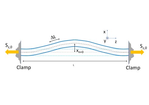
Figure 1: (Color online) Schematic of a doubly-clamped device, in its fundamental flexure ($n=0$ mode). The axial force load $S_{z,0}$ is here tensile.

For these reasons, we propose to extend this modeling to the 2D case of a drum. Our aim is to produce an analytic, robust and simple expression for the geometric nonlinear Duffing coefficient, similar to the 1D solution. The modeling remains at a generic level, not introducing any specific drive fields, and applies to non-axisymmetric modes as well as to axisymmetric ones. We shall start in Section II by reviewing the beam nonlinear mathematics, and discuss the concepts and limitations of this approach. In Section III, we present the adaptation of it to a 2D axisymmetric geometry; the stress field is discussed in Section IV and the solution is given in Section V. Our results are discussed in Section VI, with a comparison to both experiments and theory from the literature.

II Beam theory basis

Let us start by recalling the basics of the geometrical nonlinear modeling of clamped beams. We first write the Euler-Bernoulli equation that applies to thin-and-long structures bernouille ; timo :

$$E_{z}I_{z}\frac{\partial^{4}f(z,t)}{\partial z^{4}}+S_{z}\frac{\partial^{2}f(z,t)}{\partial z^{2}}=-\rho A_{z}\frac{\partial^{2}f(z,t)}{\partial t^{2}},$$ (1)

with $E_{z}$ the Young’s modulus, $I_{z}$ the second moment of area, $S_{z}$ the axial force load, $\rho$ the mass density and $A_{z}$ the section area. The $z$ index refers to the axis pointing along the beam, see Fig. 1. The beam is assumed homogeneous with a constant cross section over its length $L$. The function $f(z,t)$ describes the transverse motion of the structure (in the $x$ direction), with the proper boundary conditions. This equation essentially neglects rotational inertia of beam elementary elements $\delta z$, and all shearing forces.

When dealing with small displacements, Eq. (1) is solved by a linear superposition of eigenmodes $f_{n}(z,t)$:

$$f_{n}(z,t)=x_{n}(t)\psi_{n}(z),$$ (2)

with $\psi_{n}(z)$ the mode shape of mode $n$ (no units), and corresponding mode resonance frequency $\omega_{n}$. $x_{n}(t)$ is the time-dependent motion associated with the mode; by means of a Rotating-Frame Transform, it writes $a_{n}(t)\cos(\omega t+\phi)$ with $a_{n}(t)$ a slow varying amplitude variable, nonzero only for $\omega\approx\omega_{n}$ (resonance condition). Here, $S_{z}=S_{z,0}=\sigma_{0}A_{z}$ the initially stored axial load in the structure (from uniaxial stress $\sigma_{0}$). With this convention, $S_{z}$ is negative for a tensile stored stress. Note that the quantitative value of $x_{n}(t)$ depends on the normalization choice of $\psi_{n}(z)$; in this paper we will always normalize modal functions to the maximum displacement amplitude, such that at this abscissa $z_{n}$ one gets $\psi_{n}(z_{n})=1$.

The stretching of the beam writes $S_{z}=S_{z,0}+\Delta S$ with $\left|\Delta S\right|=E_{z}A_{z}\,\Delta L/L$ and $\Delta L$ the extension crosslifshitzbook :

$$\Delta L=\frac{1}{2}\int_{0}^{L}\!\!\left(\frac{\partial f(z,t)}{\partial z}\right)^{\!2}dz,$$ (3)

expanded at lowest order in $f$. Note that from Eq. (2) for a single mode, this expression is quadratic in motion amplitude $x_{n}(t)$, thus a simple Rotating-Wave Approximation leads to an extension $\Delta L\propto a_{n}^{2}$ (the slow variable): the nonlinear stretching is essentially a static effect, which is why there is no time-delay in the relationship between $\Delta S$ and $\Delta L$. For a superposition of modes, a similar quadratic nonlinear coupling between them is obtained (see e.g. Ref. kunalNJP ).

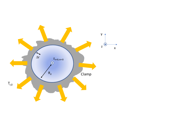
Figure 2: (Color online) Schematic of a drum device, in its fundamental flexure ($\left\{n=0,m=0\right\}$ mode). The biaxial force $2\pi R_{d}\,T_{r,0}$ is here tensile.

The basic nonlinear modeling consists then in re-injecting Eq. (3) into Eq. (1), and neglecting any other alterations due to the large motion amplitude (see discussion below). For a single mode $f\rightarrow f_{n}$, the projection of Eq. (1) onto it (i.e. multiplying the equation by $\psi_{n}$ and integrating over the beam length) leads to the definition of modal parameters:

$$\!\!m_{n} \!\!\!= \!\!\!\rho A_{z}\!\!\int_{0}^{L}\!\!\left[\psi_{n}(z)\right]^{2}dz,$$ (4)

$$\!\!k_{n} \!\!\!= \!\!\!E_{z}I_{z}\!\!\int_{0}^{L}\!\!\left[\frac{d^{2}\psi_{n}(z)}{dz^{2}}\right]^{2}\!\!\!dz-S_{z,0}\!\!\int_{0}^{L}\!\!\left[\frac{d\psi_{n}(z)}{dz}\right]^{2}\!\!\!dz,$$ (5)

$$\tilde{k}_{n} \!\!\!= \!\!\!\frac{E_{z}A_{z}}{2\,L}\!\left(\int_{0}^{L}\!\!\left[\frac{d\psi_{n}(z)}{dz}\right]^{2}\!\!\!dz\right)^{\!\!2}\!,$$ (6)

with $m_{n}$ the mode mass, $k_{n}$ the mode spring constant and $\tilde{k}_{n}$ the Duffing nonlinear parameter. The resonance frequency verifies $\omega_{n}=\sqrt{k_{n}/m_{n}}$. Including in Eq. (1) a damping and a drive term is straightforward crosslifshitzbook . The obtained equation of motion for $x_{n}$ is then the one of a harmonic oscillator plus a purely cubic nonlinear restoring term $+\tilde{k}_{n}\,x_{n}(t)^{3}$. $\tilde{k}_{n}$ is always positive, because of stretching (the mode “hardens”); in the steady-state ($a_{n}=$ constant), the resonant response measured while sweeping the drive frequency upwards will be pulled up, with the frequency at maximum amplitude $a_{n}^{max}$ given by $\omega_{n}^{res}=\omega_{n}+\beta_{n}\,(a_{n}^{max})^{2}$ with $\beta_{n}=\frac{3}{8}\omega_{n}\frac{\tilde{k}_{n}}{k_{n}}$ LLMeca ; crosslifshitzbook ; PRBEddy . The free-decay solution can also be analytically produced PRBEddy .

Beyond the agreement with experiments already mentioned, a discussion on the genesis and validity of this theory is in order. A thorough discussion of the historical developments can be found in e.g. Ref. mohammad ; nayfehbook . The first attempt to model the stretching is due to Woinowsky-Krieger Woinowsky . He considered hinged-hinged bars, and restricted his analysis to the simple approximation $\psi_{n}(z)=\sin(n\pi\,z/L)$, $n>0$ for the mode shapes. Burgreen Burgreen considered the same situation for $n=1$ only, but extended it to the case where a compressive axial load is imposed ($S_{z,0}>0$ here). Eisley Eisley proposed also a solution for the first mode of clamped-clamped beams, assuming $\psi_{1}(z)=1-\cos(2\pi z/L)$. In all of these studies, nonlinear effects stemming from inertia and curvature were neglected; their main achievement was to produce an analytic solution for the Duffing equation (written for $x_{n}[t]$) in terms of Jacobi Elliptic functions Woinowsky ; Burgreen ; Eisley . The modeling has then been adapted by Yurke et al. bush , defining modal parameters as a function of linear mode shapes $\psi_{n}(z)$ without a sinewave ansatz. This is the procedure we reproduced above; solving the Duffing equation for $x_{n}(t)$ is an extra step that we do not discuss and can be found in e.g. Refs. crosslifshitzbook ; PRBEddy ; LLMeca ; nayfehbook .

Inertia and curvature nonlinearities at large deflections have been studied by Crespo da Silva and Glynn, first for a clamped-free configuration crespo1 ; crespo2 and then for a clamped-sliding one crespo3 . It turns out that the obtained dynamics equation are of same order as the ones obtained for pure stretching (these Refs. extend the problem up to order 3 in $x_{n}$): the result is thus a similar Duffing-like behavior, and there is no a priori reason to neglect these terms in the stretching theory. Indeed, in a later series of articles, Crespo da Silva considered both extensional and curvature-inertia nonlinearities crespo4 ; crespo5 . The trial functions used for the mode shapes were here the linear solutions $\psi_{n}(z)$, the approach re-used later on since Ref. bush . His analysis demonstrated that extensional coefficients in the dynamics equation are dominant compared to the others crespo5 ; this then justifies not to take the latter into account in Eq. (6).

However, the accuracy of the Euler-Bernoulli nonlinear modeling itself remains questionable. Considering inextensional beams, only inertia and curvature nonlinear terms exist. For macroscopic cantilevers, Anderson et al. anderson showed that the first mode displays a hardening nonlinearity, while the second mode displays softening. But more recent experiments using nano-mechanical devices demonstrated that for the first mode, experiments do not match theory: the measured Duffing coefficient is very small, with even a sign change depending on aspect ratio betaRoukes . To date, this has not been explained to our knowledge. Finally, one approximation which we did not question so far is the use of the linear mode shape as trial function. While this is obviously more accurate than a simple sinewave (valid only in specific cases), it is not the exact solution of the nonlinear equation. Beyond approximate models obtained e.g. from the method of multiple scales nayfehbook , an expansion of it can be written as $f_{n}(z,t)=x_{n}(t)\psi_{n}(z)+\sum_{k>1}x_{n}(t)^{k}\delta\psi_{n}^{(k)}(z)$ with $\delta\psi_{n}^{(k)}(z)$ corrective functions matching the boundary conditions, and verifying $\delta\psi_{n}^{(k)}(z_{n})=0$ (such that $x_{n}$ remains defined as maximum amplitude deflection). It is obvious that injecting this expression in Eq. (1), the $\delta\psi_{n}^{(k)}(z)$ do generate terms that impact the nonlinear coefficients weighting $x_{n}^{2},x_{n}^{3}$ in the dynamics equation. Considering the success of the basic modeling for doubly-clamped beams, we have to assume that at least in this configuration the $\delta\psi_{n}^{(k)}(z)$ contributions remain numerically small; but to our knowledge this has not been demonstrated analytically.

The pragmatic point of the present paper is thus to adapt the very same reasoning applied to doubly-clamped beams to the case of circular drum resonators. We shall not question the theoretical limits mentioned above, but will compare our result to both theory and experiments from the literature.

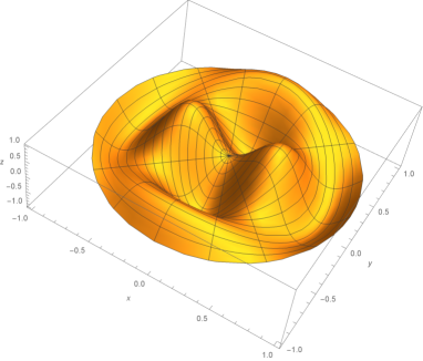
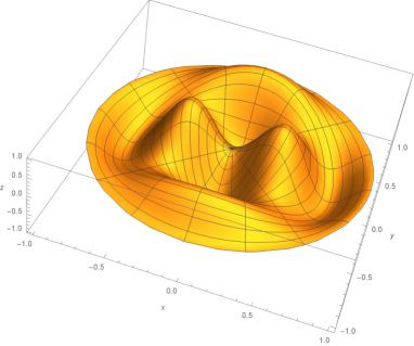
Figure 3: (Color online) Calculated mode shape $\psi_{n,m}(r,\theta)$ for mode $\left\{n=2,m=1\right\}$ (radius $R_{d}=1$). Top: high-stress limit. Bottom: low-stress limit. Both are very similar in topography.

III Formulation of the problem

We now develop the same ideas for the case of a 2D circular structure, see Fig. 2. We first remind the reader about the conventional linear theory schmidbook . The generic formalism applying to thin drums [obtained within the same reasoning as Eq. (1)] is the Kirchhoff-Love equation:

$$D_{r}\,\Delta^{2}f(r,\theta,t)+T_{r,0}\,\Delta f(r,\theta,t)=-\rho h\frac{\partial^{2}f(r,\theta,t)}{\partial t^{2}},$$ (7)

with $\Delta\cdots=\frac{1}{r}\frac{\partial}{\partial r}(r\frac{\partial\cdots}{\partial r})+\frac{1}{r^{2}}\frac{\partial^{2}\cdots}{\partial\theta^{2}}$ the Laplacian operator (here in polar coordinates), $D_{r}=\frac{1}{12}E_{r}h^{3}/(1-\nu_{r}^{2})$ the flexural rigidity in the plane of the drum ($\nu_{r}$ being Poisson’s ratio), $2\pi R_{d}\,T_{r,0}=2\pi R_{d}h\,\sigma_{0}$ the tension within the drum, $h$ its thickness and $R_{d}$ its radius. We assume materials properties $E_{r},\nu_{r},\rho,\sigma_{0}$ and thickness $h$ to be homogeneous and isotropic over the device; in Eq. (7), the $T_{r,0}$ term resulting from the biaxial stress $\sigma_{0}$ is taken negative for tensile load.

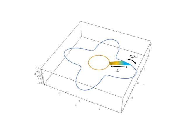
Figure 4: (Color online) Normalized stretching function $\epsilon$ plotted for mode $\left\{n=2,m=1\right\}$ in high-stress limit (with $z_{n,m}/R_{d}=1$). The stretched surface area $R_{d}\delta\theta\Delta r$ is indicated on the graph (central circle represents the drum).

In the limit of small displacements, we write:

$$f_{n,m}(r,\theta,t)=z_{n,m}(t)\psi_{n,m}(r,\theta),$$ (8)

with $\psi_{n,m}(r,\theta)=\phi_{n,m}(r)\,\cos\left(n\,\theta\right)$ the mode shapes and $z_{n,m}(t)$ the motion amplitude; now two indexes are necessary to label all 2D flexural modes of the structure. Two simple limits are considered in this paper: the high-stress case (membranes, $D_{r}=0$ with $T_{r,0}<0$ here), and the low-stress one (plates, $T_{r,0}=0$). Using the boundary conditions, the solutions write:

$$\phi_{n,m}(r)=$$ (9)

$$\!\!\!\!\!\!\!\!\!\!\frac{\mbox{BesselJ}_{n}\!\left(\frac{\lambda_{n,m}r}{R_{d}}\right)}{\mbox{BesselJ}_{n}\!\left(\frac{\lambda_{n,m}r_{n,m}}{R_{d}}\right)},$$

or

$$\!\!\!\!\!\!\!\!\!\!\frac{\mbox{BesselI}_{n}\!\left(\frac{\lambda_{n,m}r}{R_{d}}\right)-\frac{\mbox{BesselI}_{n}\!\left(\lambda_{n,m}\right)}{\mbox{BesselJ}_{n}\!\left(\lambda_{n,m}\right)}\mbox{BesselJ}_{n}\!\left(\frac{\lambda_{n,m}r}{R_{d}}\right)}{\mbox{BesselI}_{n}\!\left(\frac{\lambda_{n,m}r_{n,m}}{R_{d}}\right)-\frac{\mbox{BesselI}_{n}\!\left(\lambda_{n,m}\right)}{\mbox{BesselJ}_{n}\!\left(\lambda_{n,m}\right)}\mbox{BesselJ}_{n}\!\left(\frac{\lambda_{n,m}r_{n,m}}{R_{d}}\right)},$$

for high-stress and low-stress respectively. $\lambda_{n,m}$ is the mode parameter and $r_{n,m}$ the radial position of the maximum amplitude (occurring for given angles $\theta$ when $n\neq 0$). We give the first modes $\lambda_{n,m}$ and $r_{n,m}$ in Tab. 1 (Appendix A); the mode $\left\{n=2,m=1\right\}$ is displayed as an example in Fig. 3 for the two limits (top: high-stress, bottom: low-stress).

The stretching in 2D is a change of surface area per unit angle. This writes mathematically:

$$\frac{\delta S}{\delta\theta}=$$ (10)

$$\frac{1}{2}\int_{0}^{R_{d}}\!\!\left[\left(\frac{\partial f(r,\theta,t)}{\partial r}\right)^{\!2}+\frac{1}{r^{2}}\left(\frac{\partial f(r,\theta,t)}{\partial\theta}\right)^{\!2}\right]rdr,$$

at lowest order in $f$. Geometrically, this quantity is directly linked to the radial strain $\epsilon=\Delta r/R_{d}$ experienced by the drum at its edge: $\delta S=R_{d}\delta\theta\,\Delta r$, i.e. $\frac{\delta S(\theta,t)}{\delta\theta}=R_{d}^{2}\,\epsilon(\theta,t)$ [see Fig. 4]. Injecting the mode shape Eq. (8) into Eq. (10), one obtains:

$$\epsilon(\theta,t)=\left(\frac{z_{n,m}(t)}{R_{d}}\right)^{2}\times$$ (11)

$$\left[\frac{C_{n,m}^{(1)}+C_{n,m}^{(2)}}{2}+\frac{C_{n,m}^{(1)}-C_{n,m}^{(2)}}{2}\cos(2n\,\theta)\right],$$

where we have defined (constants with no dimensions):

$$C_{n,m}^{(1)} = \frac{1}{2}\int_{0}^{R_{d}}\!\!\left(\frac{d\phi_{n,m}(r)}{dr}\right)^{2}rdr,$$ (12)

$$C_{0,m}^{(2)} = C_{0,m}^{(1)},$$ (13)

$$C_{n,m}^{(2)} = \frac{1}{2}\int_{0}^{R_{d}}\!\frac{n^{2}}{r^{2}}\,\phi_{n,m}(r)^{2}\,rdr\,\,\,\mbox{for n$\neq 0$}.$$

The $C_{n,m}^{(1,2)}$ constants of the first modes are given in Tab. 4, Appendix C. We omit indexes $n,m$ in the labeling of $\epsilon$ for simplicity. The function Eq. (11) is plotted in Fig. 4 for mode $\left\{n=2,m=1\right\}$ in the high-stress limit.

For $n=0$, the problem is isotropic and the solution rather straightforward. However for $n\neq 0$, the stress within the drum has an extra angle-dependent component $\cos(2n\,\theta)$. Eq. (7) has thus to be modified to:

$$\!\!\!\!\!\!\!\!\!\!\!\!D_{r}\,\Delta^{2}f$$

$$+ \int_{-h/2}^{+h/2}\frac{1}{r}\frac{\partial}{\partial r}\left(\!\sigma_{r}\,r\frac{\partial f}{\partial r}\right)+\frac{1}{r^{2}}\frac{\partial}{\partial\theta}\left(\!\sigma_{\theta}\frac{\partial f}{\partial\theta}\right)dz$$

$$= -\rho h\frac{\partial^{2}f}{\partial t^{2}},$$

with $\sigma_{r}(r,\theta,z,t),\sigma_{\theta}(r,\theta,z,t)$ the superposition of the initial biaxial stress $\sigma_{0}$ plus the elastic response of the drum to the strain $\epsilon$, Eq. (11). These stress components are defined below. As for beams, we neglect any other nonlinear contribution arising from the large motion amplitude; shear stresses (e.g. $\sigma_{r,\theta}$ component) are not taken into account in Kirchhoff-Love theory (as in Euler-Bernoulli).

IV Stress field

The next step is thus to compute the stress field within the device; this is indeed the extra difficulty that arises in 2D. As for beams, we assume that the stretching is adiabatic, i.e. the stress/strain relation can be treated in a time-independent manner. The total stress field is the sum of a homogeneous contribution, plus the response to the angle-dependent stretching. The former is straightforward (e.g. Appendix B):

$$\sigma_{r}^{hom.} = \sigma_{0}-E_{r}\frac{1}{1-\nu_{r}}\epsilon^{hom.},$$ (15)

$$\sigma_{\theta}^{hom.} = \sigma_{0}-E_{r}\frac{1}{1-\nu_{r}}\epsilon^{hom.},$$ (16)

$$\sigma_{z}^{hom.} = 0,$$ (17)

with all shears equal to zero $\sigma_{r,z}=\sigma_{r,\theta}=\sigma_{\theta,z}=0$. The $-$ sign above comes from our stress convention. In the problem at stake, from Eq. (11) we have $\epsilon^{hom.}=\left(\frac{z_{n,m}}{R_{d}}\right)^{2}\left[\frac{C_{n,m}^{(1)}+C_{n,m}^{(2)}}{2}\right]$. This stress field component remains biaxial.

To compute the angle-dependent term, we start with an ansatz for the associated displacement field $\left\{u_{r},u_{\theta},u_{z}\right\}$:

$$u_{r} = R_{d}\,f_{r}(r,z)\,\epsilon^{angl.}(\theta),$$ (18)

$$u_{\theta} = R_{d}\,f_{\theta}(r,z)\,\frac{d\epsilon^{angl.}(\theta)}{d\theta},$$ (19)

$$u_{z} = h\,f_{z}(r,z)\,\epsilon^{angl.}(\theta),$$ (20)

with $\epsilon^{angl.}=\left(\frac{z_{n,m}}{R_{d}}\right)^{2}\left[\frac{C_{n,m}^{(1)}-C_{n,m}^{(2)}}{2}\cos(2n\,\theta)\right]$. These expressions are then injected in the well-known equilibrium equations of elasticity theory (see e.g. clelandbook ), neglecting inertial terms; these are given for the interested reader in Appendix B.

Introducing reduced variables $\tilde{r}=r/R_{d}$ and $\tilde{z}=z/h$, one can show that the displacement functions have to be written, at lowest order in $h/R_{d}\ll 1$ (thin structure):

$$f_{r}(\tilde{r},\tilde{z}) = c_{r}(\tilde{r})\,\left|\tilde{z}\right|+b_{r}(\tilde{r})+a_{r}(\tilde{r})\,\left(\tilde{z}\right)^{2}\left[\frac{h}{R_{d}}\right]^{2}\!\!\!,$$ (21)

$$f_{\theta}(\tilde{r},\tilde{z}) = c_{\theta}(\tilde{r})\,\left|\tilde{z}\right|+b_{\theta}(\tilde{r})+a_{\theta}(\tilde{r})\,\left(\tilde{z}\right)^{2}\left[\frac{h}{R_{d}}\right]^{2}\!\!\!,$$ (22)

$$f_{z}(\tilde{r},\tilde{z}) = c_{z}(\tilde{r})\,\left|\tilde{z}\right|+b_{z}(\tilde{r})+a_{z}(\tilde{r})\,\left(\tilde{z}\right)^{2}\left[\frac{h}{R_{d}}\right]^{2}$$ (23)

$$\!\!\!\!\!\!\!\!\!\!\!\!\!\!\!\!\!\!\!\!\!\!\!\!\!\!\!\!\!\!\!\!\!\!\!\!\!-\frac{1}{4(1-\nu_{r})}\left(\frac{c_{r}(\tilde{r})-(2n)^{2}\,c_{\theta}(\tilde{r})+\tilde{r}\,\frac{dc_{r}(\tilde{r})}{d\tilde{r}}}{\tilde{r}}\right)\!\left(\tilde{z}\right)^{2}\!\!.$$

For the nine (adimensional) functions $a_{X},b_{X},c_{X}$ ($X=r,\theta,z$) of the $\tilde{r}$-variable, we then chose the following ansatz:

$$b_{r}(\tilde{r}) = b_{r,0}\,\tilde{r}^{\alpha},$$ (24)

$$b_{\theta}(\tilde{r}) = b_{\theta,0}\,\tilde{r}^{\alpha},$$ (25)

$$c_{r}(\tilde{r}) = c_{r,0}\,\tilde{r}^{\alpha},$$ (26)

$$c_{\theta}(\tilde{r}) = c_{\theta,0}\,\tilde{r}^{\alpha},$$ (27)

$$b_{z}(\tilde{r}) = b_{z,0}\,\tilde{r}^{\alpha-1},$$ (28)

$$c_{z}(\tilde{r}) = c_{z,0}\,\tilde{r}^{\alpha-1},$$ (29)

$$a_{r}(\tilde{r}) = a_{r,0}\,\tilde{r}^{\alpha-2},$$ (30)

$$a_{\theta}(\tilde{r}) = a_{\theta,0}\,\tilde{r}^{\alpha-2},$$ (31)

and:

$$a_{z}(\tilde{r})=a_{z,0}\,\tilde{r}^{\alpha-3},$$ (32)

which leads to seven equations linking the above introduced constants. Obviously, $\alpha\geq 3$ to guarantee a physical solution.

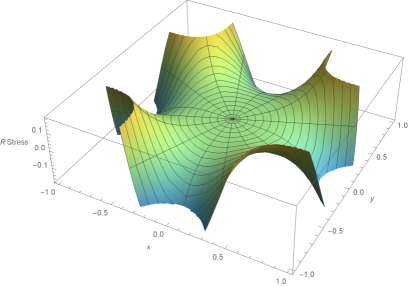
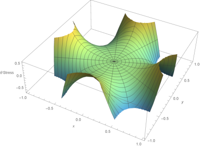
Figure 5: (Color online) Stress components $\sigma_{r}^{angl.}$ (top) and $\sigma_{\theta}^{angl.}$ (bottom) computed for mode $\left\{n=2,m=1\right\}$ in the high-stress limit. The graph has been normalized to $E_{r}=1$, $R_{d}=1$, and $z_{n,m}/R_{d}=1$ (using $\nu_{r}=+0.3$).

Three more equations are obtained from the stress boundary conditions on the surface of the drum: $\sigma_{z}(r,\theta,z=\pm h/2)=0$, $\sigma_{r,z}(r,\theta,z=\pm h/2)=0$ and $\sigma_{\theta,z}(r,\theta,z=\pm h/2)=0$. The last relation is obtained from the stretching on the periphery, equating the radial strain $\partial u_{r}/\partial r$ to $\epsilon^{angl.}$ at $r=R_{d}$ (see Fig. 4). Solving the problem under Mathematica^®, we list the constants appearing in Eqs. (25-32) in Tab. 2, Appendix B (as a function of $n$ and $\nu_{r}$). The exponent $\alpha$ is found to be $2n+1$, reminding $n\neq 0$.

The $\theta$-dependent stress field can finally be calculated. The normal components write, in the limit $h/R_{d}\approx 0$:

$$\sigma_{r}^{angl.} = -E_{r}\,\eta_{r}^{(n)}(\nu_{r})\left(\frac{r}{R_{d}}\right)^{\alpha-1}\!\!\epsilon^{angl.},$$ (33)

$$\sigma_{\theta}^{angl.} = -E_{r}\,\eta_{\theta}^{(n)}(\nu_{r})\left(\frac{r}{R_{d}}\right)^{\alpha-1}\!\!\epsilon^{angl.},$$ (34)

$$\sigma_{z}^{angl.} = 0.$$ (35)

The functions $\eta_{r}^{(n)}(\nu_{r})$ and $\eta_{\theta}^{(n)}(\nu_{r})$ with $n\neq 0$ are defined by:

$$\eta_{r}^{(n\neq 0)}(\nu_{r}) = \frac{1+2n-2(1+n)\nu_{r}}{(1+2n)(1+\nu_{r})},$$ (36)

$$\eta_{\theta}^{(n\neq 0)}(\nu_{r}) = -\frac{3+4n}{(1+2n)(1+\nu_{r})}.$$ (37)

The only nonzero shear stress is $\sigma_{r,\theta}$ (see Appendix B). It shall be neglected in this modified Kirchhoff-Love theory, as already stated. As an example, the computed (normalized) stress components are displayed in Fig. 5 for mode $\left\{n=2,m=1\right\}$, in the high-stress limit.

Angle-dependent terms Eqs. (33-35) and homogeneous terms Eqs. (15 -17) can be rewritten in a compact form:

$$\!\!\!\!\!\!\!\!\!\!\!\!\!\!\!\sigma_{r} \!\!\!= \!\!\!\sigma_{0}-E_{r}\!\!\left[\eta_{r}^{(0)}(\nu_{r})\,\epsilon^{hom.}+\eta_{r}^{(n)}(\nu_{r})\left(\frac{r}{R_{d}}\right)^{2n}\!\!\!\!\epsilon^{angl.}\right]\!,$$ (38)

$$\!\!\!\!\!\!\!\!\!\!\!\!\!\!\!\sigma_{\theta} \!\!\!= \!\!\!\sigma_{0}-E_{r}\!\!\left[\eta_{\theta}^{(0)}(\nu_{r})\,\epsilon^{hom.}+\eta_{\theta}^{(n)}(\nu_{r})\left(\frac{r}{R_{d}}\right)^{2n}\!\!\!\!\epsilon^{angl.}\right]\!,$$ (39)

$$\!\!\!\!\!\!\!\!\!\!\!\!\!\!\!\sigma_{z} \!\!\!= \!\!\!0,$$ (40)

provided we define $\eta_{r}^{(0)}(\nu_{r})=\eta_{\theta}^{(0)}(\nu_{r})=\eta^{(0)}(\nu_{r})=1/(1-\nu_{r})$. The stress is still planar, and independent of $z$, but $\sigma_{r}\neq\sigma_{\theta}$ and is neither homogeneous nor isotropic. Injecting these in Eq. (III), we can now solve the problem at hand.

V Mode parameters

Having found the stress field, we can now project Eq. (III) on a given mode $\left\{n,m\right\}$. We thus define modal parameters:

$${\cal M}_{n,m} = \rho h\int_{0}^{2\pi}\!\!\int_{0}^{R_{d}}\!\left[\psi_{n,m}(r,\theta)\right]^{2}rdrd\theta,$$ (41)

$${\cal K}_{m,n} = D_{r}\int_{0}^{2\pi}\!\!\int_{0}^{R_{d}}\!\left[\psi_{n,m}(r,\theta)\Delta^{2}\psi_{n,m}(r,\theta)\right]\,rdrd\theta$$ (42)

$$\!\!\!\!\!\!\!\!\!\!\!\!\!\!\!\!\!\!\!\!\!\!\!\!\!\!\!\!\!\!\!\!+ \!\!\!\!\!\!\!\!\!\!\!\!\!\!\!T_{r,0}\int_{0}^{2\pi}\!\!\int_{0}^{R_{d}}\left[\psi_{n,m}(r,\theta)\Delta\psi_{n,m}(r,\theta)\right]\,rdrd\theta,$$

in a similar fashion to Eqs. (4 - 5). The resonance frequencies $\omega_{n,m}=\sqrt{{\cal K}_{m,n}/{\cal M}_{n,m}}$ reduce to:

$$\omega_{n,m}=$$ (43)

$$\sqrt{\frac{\left|T_{r,0}\right|}{\rho\,h}}\left(\frac{\lambda_{n,m}}{R_{d}}\right)$$

or

$$\sqrt{\frac{D_{r}}{\rho\,h}}\left(\frac{\lambda_{n,m}}{R_{d}}\right)^{\!2},$$

in the limit of high-stress and low-stress devices, respectively. We give mass and spring values for the first modes in Tab. 3, Appendix C.

Beyond the usual linear coefficients, the Duffing term analogous to Eq. (6) finally writes:

$$\!\!\!\!\tilde{{\cal K}}_{n,m} = -\frac{E_{r}h}{R_{d}^{2}}\times$$

$$\!\!\!\!\!\!\!\!\!\!\!\!\!\!\!\!\!\!\!\!\!\!\!\!\!\!\!\left[\frac{C_{n,m}^{(1)}+C_{n,m}^{(2)}}{2}\,\eta^{(0)}(\nu_{r})\int_{0}^{2\pi}\!\!\!\int_{0}^{1}\left[\psi_{n,m}(\tilde{r},\theta)\Delta\psi_{n,m}(\tilde{r},\theta)\right]\,\tilde{r}d\tilde{r}d\theta\right.$$

$$\!\!\!\!\!\!\!+ \!\!\!\!\!\!\!\left.\frac{C_{n,m}^{(1)}-C_{n,m}^{(2)}}{2}\times\right.$$

$$\left.\left(\eta_{r}^{(n)}(\nu_{r})\frac{\pi}{2}\int_{0}^{1}\frac{\phi_{n,m}(\tilde{r})}{\tilde{r}}\frac{d}{d\tilde{r}}\left(\tilde{r}^{2n+1}\,\frac{d\phi_{n,m}(\tilde{r})}{d\tilde{r}}\right)\tilde{r}d\tilde{r}\right.\right.$$

$$+ \left.\left.\eta_{\theta}^{(n)}(\nu_{r})\frac{n^{2}\pi}{2}\int_{0}^{1}\frac{\tilde{r}^{2n+1}\,\phi_{n,m}(\tilde{r})^{2}}{\tilde{r}^{3}}\tilde{r}d\tilde{r}\right)\right],$$

with the integrals written in normalized units $\tilde{r}=r/R_{d}$ (no dimensions).

Numerical values for the integrals defining the coefficients $\tilde{{\cal K}}_{n,m}$ are listed and discussed for the first modes in Appendix C, Tabs. 5 and 6. For beams, Eq. (6) leads to a scaling of the Duffing parameter $\tilde{k}_{n}\propto E_{z}A_{z}/L^{3}$. Similarly here, Eq. (V) leads to $\tilde{{\cal K}}_{n,m}\propto E_{r}(h\,2\pi R_{d})/R_{d}^{3}$; in both cases, the Duffing effect is a stiffening.

VI Discussion

As for beams, there is a tremendous literature on nonlinear plates and membranes. In Section II, we reviewed the beam-based modeling in order to clarify the basis of the theory that we adapt here in 2D; for a detailed account of historical developments in the modeling of drums, we direct the interested reader to Refs. Amabili_book ; Pai_book ; nayfehbook .

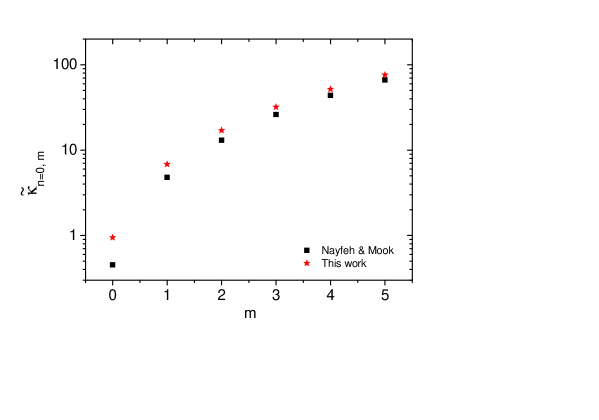
Figure 6: (Color online) Comparison between our theory (stars) and Ref. nayfehbook (squares) in units of $E_{r}h/R_{d}^{2}$, computed for $\nu=1/3$; see text.

Let us however illustrate the theoretical state-of-art with typical results from the field of MEMS and NEMS. In the last decades, the fast development of micro and nano-mechanics has been an impetus to new theoretical support, especially using modern numerical computation capabilities. Especially, the use of electrostatic actuation has been directly incorporated in the modeling (e.g. Ref. kozinsky for beam-based structures). For clamped circular plates, the conventional approach is to reduce the problem to a system of coupled ordinary differential equations, and ultimately rely on numerical methods for predictions Vogl1 ; Vogl2 . Indeed, numerical integration of nonlinear equations including electrostatic drives has proven to be an extremely efficient tool for fitting experimental data; this is the procedure followed in Ref. Sajadi to access values of the Young’s moduli in graphene membranes.

In contrast, our modeling remains at a generic level, not introducing any specific drive fields: we model only the stretching effect with no hypothesis on the origin of in-built stress. The aim is to produce an analytic expression for the Duffing coefficient. Besides, all these works deal with axisymmetric modes; Eq. (V) applies to any $\left\{n,m\right\}$.

From Ref. nayfehbook , we reproduce here the analytical modeling of axisymmetric modes. The nonlinear coefficient $\tilde{{\cal K}}_{n=0,m}^{norm}$ normalized to $E_{r}h/R_{d}^{2}$ is written as:

$$\!\!\!\!\!\tilde{{\cal K}}_{0,m}^{norm}=\!\sum_{k=1}^{\infty}\frac{\left[\int_{0}^{1}\left(d\phi_{0,m}[\tilde{r}]/d\tilde{r}\right)^{2}\mbox{BesselJ}_{1}\!\left(\zeta_{k}\tilde{r}\right)d\tilde{r}\right]^{2}}{\left(\zeta_{k}^{2}-1+\nu^{2}\right)\left[\mbox{BesselJ}_{1}\!\left(\zeta_{k}\right)\right]^{2}},$$ (45)

with the $\zeta_{k}$ parameters tabulated for $\nu=1/3$ therein ($k>0$ integer) nayfehcorr . Comparison with our expression is given in Fig. 6, summing up to $k=12$. In the displayed range, this leads to a numerical accuracy better than the size of the symbols. The two models converge towards each other for large $m$, with our numerical value above the one of Ref. nayfehbook ; for $m>1$ the difference is less than about $30~{}\%$.

Beyond comparison to existing theory, we shall assess the validity of our modeling by comparing it to benchmark measured devices from the literature in their $\left\{n=0,m=0\right\}$ resonance: a MEMS type silicon-nitride membrane in the high-stress limit, a top-down graphene NEMS device (low stress) and finally an aluminum drumhead NEMS that is typically used in quantum electronics experiments.

In Ref. DuffWeig the nonlinear behavior of a square-like silicon nitride drum has been studied. From Fig. 1 (b) of this article, we infer a Duffing parameter normalized to the mode mass of about $\tilde{{\cal K}}_{0,0}/{\cal M}_{0,0}\approx+1.5\,10^{23}~{}$m^-2s^-2. This fits the data for weak enough excitations; with larger drives, other nonlinear features kick in DuffWeig . Even though the initial stress $\sigma_{0}$ stored in the structure is not very high (110 MPa), the device is well within the membrane limit. Looking at Fig. 2 (a) from Ref. DuffWeig which displays the optically measured pattern of the first mode, it appears that it can be accurately approximated by a circular shape of radius $R_{d}\approx 210~{}\mu$m. From the parameters given in the publication (supplementary material, $E_{r}=240~{}$GPa, $\rho=3200~{}$kg/m³, thickness $h=480~{}$nm), taking a standard Poisson ratio of $\nu_{r}=+0.3$, we obtain $\tilde{{\cal K}}_{0,0}/{\cal M}_{0,0}\approx+1.2\,10^{23}~{}$m^-2s^-2. The corresponding mode resonance frequency calculated is 338 kHz, matching also consistently the measured 321 kHz.

In Ref. DuffVdZ the nonlinear behavior of a (multilayer) graphene drum has been studied. The reported stored stress is very low (about 5 MPa), and the device is better described in the plate limit. From parameters quoted in the publication ($E_{r}\approx 700~{}$GPa, $\rho=600~{}$kg/m³, $R_{d}=2.5~{}\mu$m, $h=5~{}$nm, neglecting the Poisson ratio) we compute $\tilde{{\cal K}}_{0,0}/{\cal M}_{0,0}\approx+3.3\,10^{31}~{}$m^-2s^-2 for a resonance frequency of 12.8 MHz. Again, this is in close agreement with measured values of $+2.\,10^{31}~{}$m^-2s^-2 and 14.5 MHz respectively, given in the publication for the zero DC voltage bias limit.

In Ref. DylanPRX , the nonlinear dynamics of an opto-mechanical system consisting of an aluminum drumhead device coupled to a microwave cavity has been studied. The device is about 8.5$~{}\mu$m in radius and 170 nm in thickness (Appendix of Ref. DylanPRX ), and displays a resonance frequency for the fundamental out-of-plane flexure of 6.8 MHz. The in-built stress $\sigma_{0}$ is not accurately known, but should be in the range $0-60~{}$MPa. We take for aluminum the bulk values $E_{r}=70~{}$GPa, $\rho=2700~{}$kg/m³ and $\nu_{r}=+0.35$. The Duffing parameter that is fit onto the mechanical frequency shift (Fig. 4 of Ref. DylanPRX ) is about $\tilde{{\cal K}}_{0,0}/{\cal M}_{0,0}\approx+7.\,10^{27}~{}$m^-2s^-2. This matches within $\pm 50~{}\%$ the theoretical estimate based on our modeling, for high-stress and low-stress limits, with a calculated frequency matching 6.7 MHz.

VII Conclusion

Following the same methodology as for beams, we present a theory describing the geometrical (stretching) nonlinearity of drum devices. The basic hypotheses are to neglect any other nonlinear features apart from the extra tensile stress, to neglect shearing forces, and to treat the stretching as a static effect. Two limits are considered for numerical estimates: high-stress (membranes) and low-stress (plates), but the mathematical description is written in a generic fashion. The difficulty lies in the calculation of the stress profile induced in the stretched drum for non-axisymmetric modes; the analytic solution however exists in the limit of a thin structure.

We thus present a simple and fully analytic modeling of the Duffing nonlinear coefficient $\tilde{{\cal K}}_{n,m}$ of circular plates and membranes. Only the knowledge of the mode shapes is necessary for the calculation of $\tilde{{\cal K}}_{n,m}$, through simple integrals evaluation; the first numerical values are given in Appendix. No hypotheses are made on the drive schemes, neither on the nature of the in-built biaxial stress. The theory is compared to existing analytics from Ref. nayfehbook , and to benchmark experimental data DuffWeig ; DuffVdZ ; DylanPRX . In both cases, the agreement is good.

Further comparison with experiments should be done with higher modes, especially non-axisymmetric ones ($n\neq 0$). Besides, the presented theory can be in principle extended to mode-coupling kunalNJP ; NanoRoukes ; an experimental and theoretical study of this regime would definitely assess the validity of the presented mathematical methods.

VIII Data availability

Data sharing is not applicable to this article as no new data were created or analyzed in this study.

Appendix A Mode parameters

In the Table below we give the first modes $\lambda_{n,m}$ and $r_{n,m}$ parameters for both high-stress (H.S.) and low-stress (L.S.) limits. Inserting these in Eqs. (9) one can easily compute the corresponding mode shapes (see Fig. 3 for an example).

mode $\left\{n,m\right\}$	H.S. $\lambda_{n,m}$	H.S. $r_{n,m}$		L.S. $\lambda_{n,m}$	L.S. $r_{n,m}$
$\left\{0,0\right\}$	2.40483	0.		3.19622	0.
$\left\{0,1\right\}$	5.52008	0.		6.30644	0.
$\left\{1,0\right\}$	3.83171	0.4805123		4.61090	0.4102482
$\left\{1,1\right\}$	7.01559	0.2624418		7.79927	0.2358243
$\left\{0,2\right\}$	8.65373	0.		9.43950	0.
$\left\{2,0\right\}$	5.13562	0.5947163		5.90568	0.5258299
$\left\{1,2\right\}$	10.1735	0.1809784		10.9581	0.1680282
$\left\{2,1\right\}$	8.41724	0.3628549		9.19688	0.3319174
$\cdots$	$\cdots$	$\cdots$		$\cdots$	$\cdots$

Table 1: First mode parameters. Left: high-stress (H.S.), right: low-stress (L.S.). For $n=0$ modes, the maximum amplitude is at the center ($r_{0,m}=0$).

Appendix B Stress field solution

We remind the reader basics of elasticity theory expressed in cylindrical coordinates. The strain fields can be written in terms of the displacement fields:

$$\epsilon_{r} = \frac{\partial u_{r}}{\partial r},$$

$$\epsilon_{\theta} = \frac{u_{r}}{r}+\frac{1}{r}\frac{\partial u_{\theta}}{\partial\theta},$$

$$\epsilon_{z} = \frac{\partial u_{z}}{\partial z},$$

for the normal components, and:

$$2\epsilon_{r,\theta} = \frac{\partial u_{\theta}}{\partial r}-\frac{u_{\theta}}{r}+\frac{1}{r}\frac{\partial u_{r}}{\partial\theta},$$

$$2\epsilon_{r,z} = \frac{\partial u_{r}}{\partial z}+\frac{\partial u_{z}}{\partial r},$$

$$2\epsilon_{\theta,z} = \frac{1}{r}\frac{\partial u_{z}}{\partial\theta}+\frac{\partial u_{\theta}}{\partial z},$$

for the shear strains.

For an isotropic homogeneous Hookean material, we have:

$$\bordermatrix{&\cr&\sigma_{r}\cr&\sigma_{\theta}\cr&\sigma_{z}\cr&\sigma_{r,\theta}\cr&\sigma_{r,z}\cr&\sigma_{\theta,z}\cr}=\frac{E_{r}}{(1+\nu_{r})(1-2\nu_{r})}\bordermatrix{&\cr&{\cal H}\cr}\bordermatrix{&\cr&\epsilon_{r}\cr&\epsilon_{\theta}\cr&\epsilon_{z}\cr&2\epsilon_{r,\theta}\cr&2\epsilon_{r,z}\cr&2\epsilon_{\theta,z}\cr}$$

with $({\cal H})=$

$$\bordermatrix{&&&&&&\cr&1-\nu_{r}&\nu_{r}&\nu_{r}&0&0&0\cr&\nu_{r}&1-\nu_{r}&\nu_{r}&0&0&0\cr&\nu_{r}&\nu_{r}&1-\nu_{r}&0&0&0\cr&0&0&0&\frac{1-2\nu_{r}}{2}&0&0\cr&0&0&0&0&\frac{1-2\nu_{r}}{2}&0\cr&0&0&0&0&0&\frac{1-2\nu_{r}}{2}\cr}$$

for the relationship between stresses $(\sigma)$ and strains $(\epsilon)$.

The equilibrium equations then write:

$$\frac{\partial\sigma_{r}}{\partial r}+\frac{1}{r}\frac{\partial\sigma_{r,\theta}}{\partial\theta}+\frac{1}{r}\left(\sigma_{r}-\sigma_{\theta}\right)+\frac{\partial\sigma_{r,z}}{\partial z} = 0,$$

$$\frac{\partial\sigma_{r,\theta}}{\partial r}+\frac{1}{r}\frac{\partial\sigma_{\theta}}{\partial\theta}+2\frac{\sigma_{r,\theta}}{r}+\frac{\partial\sigma_{\theta,z}}{\partial z} = 0,$$

$$\frac{\partial\sigma_{r,z}}{\partial r}+\frac{1}{r}\frac{\partial\sigma_{\theta,z}}{\partial\theta}+\frac{\sigma_{r,z}}{r}+\frac{\partial\sigma_{z}}{\partial z} = 0,$$

when neglecting the inertial terms.

The solution for the homogeneous stretching component is straightforward. The well-known displacement field simply writes:

$$f_{r}(r,z) = r,$$

$$f_{\theta}(r,z) = 0,$$

$$f_{z}(r,z) = -\frac{2\nu_{r}}{1-\nu_{r}}z,$$

with $u_{r}=f_{r}\,\epsilon^{hom.},u_{\theta}=0,u_{z}=f_{z}\,\epsilon^{hom.}$ by definition. Then $\epsilon_{r}=\epsilon_{\theta}=\epsilon^{hom.}$ and $\epsilon_{z}=-2\nu_{r}\epsilon^{hom.}/(1-\nu_{r})$; all other components of the strain field are zero. Clearly, imposing a radial stretching also causes nonzero tangential and vertical strains. The resulting stresses are Eqs. (15-17).

The case of the angular-dependent component is much more complex. Injecting in the above the ansatz Eqs. (18-20) for the displacement fields, and writing the problem in reduced coordinates, we realize that the solution should be of the type Eqs. (21-23) at lowest order in $h/R_{d}$. The symmetry of the drum with respect to $z\rightarrow-z$ has been used. To further reduce the problem, another ansatz is needed for the $\tilde{r}$-dependent functions introduced in the writing of the solution: we assume them to be power laws, Eqs. (25-32). Taking into account the boundary conditions (no $z$-component stress on the surface of the drum, and fixed radial strain at the periphery), we end up with the constants listed in Tab. 2.

The $\epsilon_{0}$ term is simply the prefactor of the angular-dependent strain, $\epsilon^{angl.}=\epsilon_{0}\cos(2n\,\theta)$. The stresses do depend on $\tilde{z}^{2}$. However, in the limit $h/R_{d}\rightarrow 0$ these terms vanish and the stress components are homogeneous within the thickness of the drum. Also $\sigma_{z}=0$: the stress state is planar. The two normal components $\sigma_{r}^{angl.},\sigma_{\theta}^{angl.}$ Eqs. (33-34) are displayed in Fig. 5 for mode $\left\{n=2,m=1\right\}$ in the high-stress limit.

Furthermore, the only nonzero shear stress component is $\sigma_{r,\theta}^{angl.}$. It then writes:

$$\sigma_{r,\theta}^{angl.}=-E_{r}\frac{n(-3+\nu_{r})+(-2+\nu_{r})}{(1+2n)(1+\nu_{r})}\left(\frac{r}{R_{d}}\right)^{2n}\epsilon_{0}\sin(2n\,\theta),$$

with the $-$ sign matching our stress convention (tensile). It is neglected in the presented modeling.

Parameter	Expression
$b_{r,0}$	$\epsilon_{0}/(1+2n)$
$b_{\theta,0}$	$b_{r,0}\,2(1+n)(2-\nu_{r})/(2n)^{2}$
$c_{r,0}$	$0$
$c_{\theta,0}$	$0$
$b_{z,0}$	$0$
$c_{z,0}$	$b_{r,0}\,2(1+n)\nu_{r}$
$a_{r,0}$	$-b_{r,0}\,2[(1+n)(2-\nu_{r})-n^{2}]$
$a_{\theta,0}$	$b_{r,0}\,n[1-4(1+n)(2-\nu_{r})/(2n)^{2}]$
$a_{z,0}$	$0$
$\alpha$	$2n+1$
$\epsilon_{0}$	$\left(\frac{z_{n,m}}{R_{d}}\right)^{2}\frac{C_{n,m}^{(1)}-C_{n,m}^{(2)}}{2}$

Table 2: Strain coefficients of the angular-dependent contribution, as a function of $n,\nu_{r}$. $\epsilon_{0}$ is the amplitude of the $\cos(2n\,\theta)$ stretching term.

Appendix C Mass, spring and Duffing parameters

In this Appendix we give numerical estimates for mass, spring constant and nonlinear parameters calculated for the first modes, in the two simple limits of high-stress and low-stress.

mode $\left\{n,m\right\}$	H.S. $M_{n,m}$	H.S. $K_{n,m}$		L.S. $M_{n,m}$	L.S. $K_{n,m}$
$\left\{0,0\right\}$	0.269513	0.779325		0.182834	9.54057
$\left\{0,1\right\}$	0.115780	1.763983		0.101896	80.5872
$\left\{1,0\right\}$	0.239561	1.758616		0.184581	41.7156
$\left\{1,1\right\}$	0.133016	3.273413		0.119933	221.883
$\left\{0,2\right\}$	0.073686	2.759075		0.067543	268.132
$\left\{2,0\right\}$	0.243735	3.214208		0.200046	121.669
$\left\{1,2\right\}$	0.092082	4.765268		0.085466	616.168
$\left\{2,1\right\}$	0.155586	5.511635		0.142446	509.546
$\cdots$	$\cdots$	$\cdots$		$\cdots$	$\cdots$

Table 3: Mass and spring constant for the first modes (norm. integrals, see text). Left: high-stress (H.S.) and right: low-stress (L.S.).

For this purpose, we re-write the relevant integrals in an adimensional form such that:

$${\cal M}_{n,m}=\rho h\pi R_{d}^{2}\,M_{n,m},$$

and:

$${\cal K}_{m,n}=$$

$$\frac{2\pi R_{d}\left|T_{r,0}\right|}{R_{d}}\,K_{n,m}$$

or

$$\frac{D_{r}\,2\pi R_{d}}{R_{d}^{3}}\,K_{n,m},$$

in the high-stress and low-stress limits, respectively. $\rho h\pi R_{d}^{2}$ is the mass of the drum (in kg), and $2\pi R_{d}\left|T_{r,0}\right|$ the force tensioning the device at the periphery (in N, equivalent to $S_{z}$ for the beam case, see Figs. 1 and 2). Similarly, the flexural rigidity times perimeter $D_{r}\,2\pi R_{d}$ replaces the product $E_{z}I_{z}$ of the Euler-Bernoulli modeling. Numerical values for $M_{n,m}$ and $K_{n,m}$ are listed in Tab. 3. Note that the mass parameters $M_{n,m}$ obtained in both high-stress and low-stress limits are very close. Resonance frequencies are then given by Eq. (43).

mode $\left\{n,m\right\}$	H.S. $C_{n,m}^{(1)}$	H.S. $C_{n,m}^{(2)}$		L.S. $C_{n,m}^{(1)}$	L.S. $C_{n,m}^{(2)}$
$\left\{0,0\right\}$	0.389664	0.389664		0.316669	0.316669
$\left\{0,1\right\}$	0.881992	0.881992		0.851698	0.851698
$\left\{1,0\right\}$	1.139994	0.618625		0.920002	0.630386
$\left\{1,1\right\}$	2.60152	0.671898		2.50136	0.682519
$\left\{0,2\right\}$	1.37954	1.37954		1.34492	1.34492
$\left\{2,0\right\}$	1.62609	1.58811		1.31374	1.62645
$\left\{1,2\right\}$	4.07293	0.692365		3.96830	0.696559
$\left\{2,1\right\}$	3.71904	1.79259		3.55652	1.83054
$\cdots$	$\cdots$	$\cdots$		$\cdots$	$\cdots$

Table 4: Nonlinear coefficients $C_{n,m}^{(1,2)}$ computed for the first modes. Left: high-stress (H.S.) and right: low-stress (L.S.). Note the specificity of $n=0$ modes (by definition $C_{0,m}^{(1)}=C_{0,m}^{(2)}$, no angular dependence of strain/stress).

In Tab. 4 we give the stretching $C_{n,m}^{(1,2)}$ constants (no units) calculated for the first modes. High-stress and low-stress cases are again presented; the obtained numerical values in the two limits are very similar. As an illustrative example, the stretching function $\epsilon$ calculated for mode $\left\{n=2,m=1\right\}$ in the high-stress limit is presented in Fig. 4 (in normalized units).

mode $\left\{n,m\right\}$	H.S. $\tilde{K}_{n,m}^{(1)}$	H.S. $\tilde{K}_{n,m}^{(2)}$	H.S. $\tilde{K}_{n,m}^{(3)}$
$\left\{0,0\right\}$	0.779325	X	X
$\left\{0,1\right\}$	1.76398	X	X
$\left\{1,0\right\}$	1.75862	0.352992	-0.0598902
$\left\{1,1\right\}$	3.27341	0.578822	-0.0332539
$\left\{0,2\right\}$	2.75908	X	X
$\left\{2,0\right\}$	3.21421	0.421149	-0.0997277
$\left\{1,2\right\}$	4.76527	0.817227	-0.0230206
$\left\{2,1\right\}$	5.51164	0.607419	-0.0562541
$\cdots$	$\cdots$	$\cdots$	$\cdots$

Table 5: Nonlinear Duffing coefficients $\tilde{K}_{n,m}^{(1,2,3)}$ (no units) computed for the first modes, high-stress (H.S.) limit. Note that $\tilde{K}_{n,m}^{(1)}=K_{n,m}$ (H.S.), Tab. 3. For $n=0$ modes, $\tilde{K}_{0,m}^{(2,3)}$ are irrelevant (X above).

We finally propose numerical estimates for the nonlinear coefficients written as:

$$\tilde{{\cal K}}_{n,m} = +\frac{E_{r}\,h2\pi R_{d}}{R_{d}^{3}}\times$$

$$\!\!\!\!\!\!\!\!\!\!\!\!\!\!\!\!\!\!\!\!\!\!\left[\frac{C_{n,m}^{(1)}+C_{n,m}^{(2)}}{2}\,\eta^{(0)}(\nu_{r})\tilde{K}_{n,m}^{(1)}\,+\right.$$

$$\!\!\!\!\!\!\!\!\!\!\!\!\!\!\!\!\!\!\!\!\left.\frac{C_{n,m}^{(1)}-C_{n,m}^{(2)}}{2}\times\left(\eta_{r}^{(n)}(\nu_{r})\tilde{K}_{n,m}^{(2)}+\eta_{\theta}^{(n)}(\nu_{r})\tilde{K}_{n,m}^{(3)}\right)\right],$$

where the adimensional $\tilde{K}_{n,m}^{(1,2,3)}$ are given in Tabs. 5 and 6 (high-stress and low-stress limits respectively). Note the chosen normalization, that matches the Euler-Bernoulli formalism with $h2\pi R_{d}$ the cross-section area of the device at the clamp; in the high-stress limit, $\tilde{K}_{n,m}^{(1)}=K_{n,m}$.

From Tabs. 5 and 6, the $C_{n,m}^{(1,2)}$ values of Tab. 4 and the expressions of the functions $\eta_{r,\theta}^{(n)}(\nu_{r})$ [Eqs. (36,37) and subsequent text], one realizes that the geometrical Duffing nonlinear parameter is dominated by the homogeneous contribution. As a result, $\tilde{K}_{n,m}$ is always positive, as in the beam case. Finally, one can see that the numerical evaluations of $\tilde{K}_{n,m}^{(1,2,3)}$ are about twice larger in the high-stress limit than in the low-stress case. As such, for identical material parameters ($E_{r},\nu_{r},\rho$) except the biaxial stress $\sigma_{0}$ and identical geometry ($R_{d},h$), a membrane Duffing nonlinearity $\tilde{K}_{n,m}$ (H.S.) is approximately twice larger than for a plate (L.S.).

mode $\left\{n,m\right\}$	L.S. $\tilde{K}_{n,m}^{(1)}$	L.S. $\tilde{K}_{n,m}^{(2)}$	L.S. $\tilde{K}_{n,m}^{(3)}$
$\left\{0,0\right\}$	0.316669	X	X
$\left\{0,1\right\}$	0.851698	X	X
$\left\{1,0\right\}$	0.775194	0.205519	-0.0461452
$\left\{1,1\right\}$	1.59194	0.433603	-0.0299831
$\left\{0,2\right\}$	1.34492	X	X
$\left\{2,0\right\}$	1.47010	0.209512	-0.066682
$\left\{1,2\right\}$	2.33243	0.663581	-0.0213665
$\left\{2,1\right\}$	2.69353	0.388931	-0.0474821
$\cdots$	$\cdots$	$\cdots$	$\cdots$

Table 6: Nonlinear Duffing coefficients $\tilde{K}_{n,m}^{(1,2,3)}$ (no units) computed for the first modes, low stress (L.S.) limit. For $n=0$ modes, $\tilde{K}_{0,m}^{(2,3)}$ are irrelevant (X above).

References

- (1) A. N. Cleland and M. L. Roukes, Fabrication of high frequency nanometer scale mechanical resonators from bulk Si crystals, Appl. Phys. Lett. 69, 2653 (1996).
- (2) A. N. Cleland, Foundations of nanomechanics, Springer (2003).
- (3) Silvan Schmid, Luis Guillermo Villanueva, Michael Lee Roukes, Fundamentals of Nanomechanical Resonators, Springer (2016).
- (4) V. Kara, Y.-I. Sohn, H. Atikian, V. Yakhot, M. Loncar, K. L. Ekinci, Nanofluidics of Single-Crystal Diamond Nanomechanical Resonators, Nano Letters 15, 12, 8070-8076 (2015).
- (5) K. Jensen, J. Weldon, H. Garcia, A. Zettl, Nano Lett. 7, 11, 3508-3511 (2007).
- (6) Aneesh Koka and Henry A. Sodano, High-sensitivity accelerometer composed of ultra-long vertically aligned barium titanate nanowire arrays, Nature Communications 4, 2682 (2013).
- (7) Eric Sage, Marc Sansa, Shawn Fostner, Martial Defoort, Marc Gély, Akshay K. Naik, Robert Morel, Laurent Duraffourg, Michael L. Roukes, Thomas Alava, Guillaume Jourdan, Eric Colinet, Christophe Masselon, Ariel Brenac and Sébastien Hentz, Single-particle mass spectrometry with arrays of frequency-addressed nanomechanical resonators, Nature Communications 9, 3283 (2018).
- (8) A. D. O’Connell, M. Hofheinz, M. Ansmann, Radoslaw C. Bialczak, M. Lenander, Erik Lucero, M. Neeley, D. Sank, H. Wang, M. Weides, J. Wenner, John M. Martinis and A. N. Cleland, Quantum ground state and single-phonon control of a mechanical resonator, Nature 464, 697-703 (2010).
- (9) T. A. Palomaki, J. W. Harlow, J. D. Teufel, R. W. Simmonds, K. W. Lehnert, Coherent state transfer between itinerant microwave fields and a mechanical oscillator, Nature 495, 210 (2013).
- (10) J.-M. Pirkkalainen, S. U. Cho, Jian Li, G. S. Paraoanu, P. J. Hakonen and M. A. Sillanpää, Hybrid circuit cavity quantum electrodynamics with a micromechanical resonator, Nature 494, 211 (2013).
- (11) H. W. Ch. Postma, I. Kozinsky, A. Husain, and M. L. Roukes, Dynamic range of nanotube- and nanowire-based electromechanical systems, Appl. Phys. Lett. 86, 223105 (2005).
- (12) R. Almog, S. Zaitsev, O. Shtempluck, and E. Buks, High intermodulation gain in a micromechanical Duffing resonator, Appl. Phys. Lett. 88, 213509 (2006).
- (13) I. Mahboob and H. Yamaguchi, Bit storage and bit flip operations in an electromechanical oscillator, Nature Nanotechnology 3, 275 (2008).
- (14) Warner J. Venstra, Hidde J. R. Westra, and Herre S. J. van der Zant, Mechanical stiffening, bistability, and bit operations in a microcantilever, Appl. Phys. Lett. 97, 193107 (2010).
- (15) M. C. Cross, A. Zumdieck, Ron Lifshitz, and J. L. Rogers, Synchronization by Nonlinear Frequency Pulling, Phys. Rev. Lett. 93, 224101 (2004).
- (16) Matthew H. Matheny, Matt Grau, Luis G. Villanueva, Rassul B. Karabalin, M. C. Cross, and Michael L. Roukes, Phase Synchronization of Two Anharmonic Nanomechanical Oscillators, Phys. Rev. Lett. 112, 014101 (2014).
- (17) I. Kozinsky, H. W. Ch. Postma, I. Bargatin, and M. L. Roukes, Tuning nonlinearity, dynamic range, and frequency of nanomechanical resonators, Appl. Phys. Lett. 88, 253101 (2006).
- (18) N. Kacem, J. Arcamone, F. Perez-Murano and S. Hentz, Dynamic range enhancement of nonlinear nanomechanical resonant cantilevers for highly sensitive NEMS gas/mass sensor applications, J. Micromech. Microeng. 20, 045023 (2010).
- (19) Lily L. Li, Pavel M. Polunin, Suguang Dou, Oriel Shoshani, B. Scott Strachan, Jakob S. Jensen, Steven W. Shaw, and Kimberly L. Turner, Tailoring the nonlinear response of MEMS resonators using shape optimization, Appl. Phys. Lett. 110, 081902 (2017).
- (20) M. Defoort, Non-linear dynamics in nano-electromechanical systems at low temperatures, PhD thesis, Université de Grenoble (16/12/2014).
- (21) B. Yurke, D.S. Greywall, A.N. Pargellis, P.A. Bush, Theory of amplifier-noise evasion in an oscillator employing a nonlinear resonator, Phys. Rev. A 51, 4211 (1995).
- (22) R. Lifshitz and M.C. Cross, in Reviews of Nonlinear Dynamics and Complexity, Ed. by H. G. Schuster, Wiley-VCH (2008).
- (23) E. Collin, Yu. M. Bunkov, and H. Godfrin, Addressing geometric nonlinearities with cantilever microelectromechanical systems: Beyond the Duffing model, Phys. Rev. B 82, 235416 (2010).
- (24) K. J. Lulla, R. B. Cousins, A. Venkatesan, M. J. Patton, A. D. Armour, C. J. Mellor and J. R. Owers-Bradley, Nonlinear modal coupling in a high-stress doubly-clamped nanomechanical resonator, New Journal of Physics 14, 113040 (2012).
- (25) M. H. Matheny, L. G. Villanueva, R. B. Karabalin, J. E. Sader, and M. L. Roukes, Nonlinear Mode-Coupling in Nanomechanical Systems, Nano Lett. 13, 1622 (2013).
- (26) H. J. R. Westra, M. Poot, H. S. J. van der Zant, and W. J. Venstra, Nonlinear Modal Interactions in Clamped-Clamped Mechanical Resonators, Phys. Rev. Lett. 105, 117205 (2010).
- (27) Olivier Maillet, Xin Zhou, Rasul Gazizulin, Ana Maldonado Cid, Martial Defoort, Olivier Bourgeois, Eddy Collin, Non-linear Frequency Transduction of Nano-mechanical Brownian Motion, Phys. Rev. B 96, 165434 (2017).
- (28) L.D. Landau and E.M. Lifshitz, Theory of elasticity, Butterworth-Heinemann, Oxford 3rd Ed. (1986).
- (29) S. Timoshenko, D.H. Young, and W.H. Weaver Jr., Vibrations problems in engineering, John Wiley and Sons, fourth edition (1974).
- (30) L.D. Landau and E.M. Lifshitz, Mechanics, Elsevier Science Ltd. Third Ed. (1976).
- (31) Ali H. Nayfeh and Dean T. Mook, Nonlinear oscillations, Wiley-VCH Second Ed. (2004).
- (32) Note the misprint in Ref. nayfehbook , p. 512.
- (33) Mohammad Amin Rashidifar, Nonlinear Vibrations of Cantilever Beams and Plates, Hamburg, Anchor Academic Publishing (2015).
- (34) S. Woinowsky-Krieger, The effect of an axial force on the vibration of hinged bars, J. of Appl. Mechanics 17, 35 (1950).
- (35) D. Burgreen, Free virbrations of a pin-ended column with constant distance between pin ends, J. of Appl. Mechanics 18, 135 (1951).
- (36) J.G. Eisley, Nonlinear vibration of beams and rectangular plates, ZAMP 15, 167 (1964).
- (37) M. R. M. Crespo da Silva and C. C. Glynn, Nonlinear flexural-flexural-torsional dynamics of inextensional beams-I. Equations of motion, J. Struct. Mech. 6(4), 437 (1978).
- (38) M. R. M. Crespo da Silva and C. C. Glynn, Nonlinear flexural-flexural-torsional dynamics of inextensional beams-II. Forced motions, J. Struct. Mech. 6(4), 449 (1978).
- (39) M.R.M. Crespo da Silva and C.C. Glynn, Out-of-plane vibrations of a beam including non-linear inertia and non-linear curvature effects, Int. J. Non-Linear Mechanics 13, 261 (1979).
- (40) M.R.M. Crespo da Silva, Non-linear flexural-flexural-torsional-extensional dynamics of beams-I. Formulation, Int. J. Solids Structures 24(12), 1225 (1988).
- (41) M.R.M. Crespo da Silva, Non-linear flexural-flexural-torsional-extensional dynamics of beams-II. Response analysis, Int. J. Solids Structures 24(12), 1235 (1988).
- (42) T.J. Anderson, A.H. Nayfeh, B. Balachandran, Experimental verification of the importance of the nonlinear curvature in the response of a cantilever beam, J. of Vibration and Acoustics 118, 21 (1996).
- (43) L. G. Villanueva, R. B. Karabalin, M. H. Matheny, D. Chi, J. E. Sader, and M. L. Roukes, Nonlinearity in nanomechanical cantilevers, Phys. Rev. B 87, 024304 (2013).
- (44) M. Amabili, Nonlinear Vibrations and Stability of Shells and Plates, Cambridge University Press (2008).
- (45) A. H. Nayfeh, P. F. Pai, Linear and Nonlinear Structural Mechanics, Wiley-VCH (2004).
- (46) G. W. Vogl, A. H. Nayfeh, A reduced model for electrically actuated clamped circular plates, Journal of Micromechanics and Microengineering 315, 684-690, (2005).
- (47) G. W. Vogl, A. H. Nayfeh, Primary resonance excitation of electrically actuated clamped circular plates, Nonlinear Dynamics 47. 181-192, (2007).
- (48) B. Sajadi, F. Alijani, D. Davidovikj, J. Goosen, P. G. Steeneken, F. V. Keulen, Experimental characterization of graphene by electrostatic resonance frequency tuning, Journal of Applied Physics 122, 234302, (2017).
- (49) Fan Yang, Felix Rochau, Jana S. Huber, Alexandre Brieussel, Gianluca Rastelli, Eva M. Weig, and Elke Scheer, Spatial Modulation of Nonlinear Flexural Vibrations of Membrane Resonators, Phys. Rev. Lett. 122, 154301 (2019).
- (50) D. Davidovikj, F. Alijani, S.J. Cartamil-Bueno, H.S.J. van der Zant, M. Amabili P.G. Steeneken, Nonlinear dynamic characterization of twodimensional materials, Nature Comm. 8, 1253 (2017).
- (51) D. Cattiaux, X. Zhou, S. Kumar, I. Golokolenov, R. R. Gazizulin, A. Luck, L. Mercier de Lépinay, M. Sillanpää, A. D. Armour, A. Fefferman and E. Collin, Beyond linear coupling in microwave optomechanics, arXiv:2003.03176 (2020).