Nonparametric principal subspace regression

Abstract

In scientific applications, multivariate observations often come in tandem with temporal or spatial covariates, with which the underlying signals vary smoothly. The standard approaches such as principal component analysis and factor analysis neglect the smoothness of the data, while multivariate linear or nonparametric regression fail to leverage the correlation information among multivariate response variables. We propose a novel approach named nonparametric principal subspace regression to overcome these issues. By decoupling the model discrepancy, a simple and general two-step framework is introduced, which leaves much flexibility in choice of model fitting. We establish theoretical property of the general framework, and offer implementation procedures that fulfill requirements and enjoy the theoretical guarantee. We demonstrate the favorable finite-sample performance of the proposed method through simulations and a real data application from an electroencephalogram study.

Keywords: Factor model, nonparametric principal subspace, singular value decomposition, smoothness.

1 Introduction

In scientific applications, one is often interested in predicting a multivariate response using one or a few predictor variables. The multivariate response linear regression is a conventional way to model this type of data. The usual procedure is the ordinary least squares, equivalent to performing individual linear regression of each response variable on predictor variables, which fails to utilize the correlation information among the response variables. To incorporate the correlation information, Breiman and Friedman, (1997) proposed a multivariate shrinkage method to leverage information from the correlation structure, which helps to improve the predictive accuracy compared to the ordinary least squares.

Although multivariate response linear regression is a useful tool, it may not work properly in some applications. For example, in the electroencephalogram application presented in Section 3.2, we are interested in modelling the dynamic changes of the electroencephalogram signals detected from 64 electrodes of the scalp. For each electrode, the signal is sampled at 256 Hz per second. We plot the electroencephalogram signals from one randomly selected participant in Figure 2(a), where the curves show nonlinear patterns. This indicates that the multivariate response linear regression model may not be adequate to characterize the relationship between the common predictor time and the multivariate signals from the 64 electrodes. A natural rescue is to utilize nonparametric regression of the multivariate response variables on the common predictors. However this solution is unsatisfactory as performing individual nonparametric regressions does not capture correlations among the response variables.

Motivated by the application, we propose a new nonparametric principal subspace regression model, which allows more flexible nonlinear structures of the regression functions while takes into account the correlation among response variables of the same time. Our proposal is related to the factor models, which characterize the correlation structure in multivariate data. In factor models, the signal of interest is expressed as a linear combination of a few latent variables, and does not concern additional covariate information that may play a role in estimation or prediction. For instance, factor models are often employed in contexts such as multiple time series or correlated functional data (Engle and Watson,, 1981; Huang et al.,, 2009), where useful information may be hidden in the form of smoothness with respect to some additional covariates, e.g. temporal or spatial variable. Neglecting such information in recovery and prediction potentially hinders the quality and performance of resulting estimators. This has been noticed by Durante et al., (2014), which further proposed a locally adaptive factor process under the Bayesian framework for characterizing multivariate mean-covariance changes in continuous time, allowing locally varying smoothness in both the mean and covariance matrix of multivariate time series. However, theoretical guarantees are lacking for the approach, which may leave practitioners uncertain about the quality of resulting estimates.

In this work, we approach the problem from a different perspective that is intuitive and broadly applicable. The contributions are summarized as follows. First, we propose a new nonparametric principal subspace regression model. This not only incorporates the correlation structure among multivariate responses, but also accounts for nonlinear trend and smoothness of the data. Second, we introduce a simple two-step estimation framework, where the first step is to obtain the orthogonal left singular vectors and the second step is to estimate the nonparametric loading functions. This procedure is general and leaves flexibility in choice of model fitting. Third, we provide theoretical guarantees for the general proposal, and then present some examples of standard linear smoothers and the rates they attain when used in the general proposal. Lastly, we show that our method outperforms its counterpart, the conventional nonparametric regression, in simulations as well as an electroencephalogram study. This is not surprising because our approach significantly reduces the model complexity and risk of overfitting compared to individual nonparametric regressions.

The rest of the paper is organized as follows. In Section 2, we propose the nonparametric principal subspace regression methodology, state the main results and three important examples. We further give a specific fitting procedure for our approach. Section 3 evaluates the favorable finite-sample performance of the proposed method through simulations and a real data application from an electroencephalogram study. Proofs of main propositions and theorems as well as the statements for relevant lemmas are contained in Sections 4 and 5. Statements of auxiliary lemmas and theorems for examples are given in Section 6, whereas some additional simulation results and proofs of all lemmas and theorems for examples are deferred to the supplementary file.

2 Proposed Methodology and Theoretical Guarantees

2.1 Notation

Denote the inner product of $a,b\in\mathbb{R}^{m}$ by $\langle a,b\rangle=a^{\mathrm{\scriptscriptstyle T}}b=\sum_{i=1}^{m}a_{i}b_{i}$, where $a_{i}$ and $b_{i}$ are the $i$th components of $a$ and $b$ respectively. Let $\|\cdot\|$ be the corresponding norm induced by the inner product. Define the rescaled inner product $\langle a,b\rangle_{m}=\frac{1}{m}\langle a,b\rangle$ and the induced norm $\|\cdot\|_{m}$. For two functions $f,g\in L^{2}$, the inner product and corresponding norm bear the subscript $L^{2}$, i.e. $\langle f,g\rangle_{L^{2}}=\int_{T}f(x)g(x)dx$ and $\|f\|^{2}_{L_{2}}=\int_{T}\{f(x)\}^{2}dx$, where $T$ is the domain of $x$. Let $\|a\|_{\infty}=\max_{1\leq i\leq m}|a_{i}|$ and $\|f\|_{\infty}$ denote the sup norm of function $f\in L^{2}$. Suppose we have a matrix $M\in\mathbb{R}^{p\times n}$ with rank $r$, and its singular values satisfy $\sigma_{1}(M)\geq\sigma_{2}(M)\geq\ldots\geq\sigma_{r}(M)>\sigma_{r+1}(M)=\ldots=0$. Consider the singular value decomposition $M=U\Sigma V^{\mathrm{\scriptscriptstyle T}}$, where $U$ and $V$ are $p\times r$ and $n\times r$ matrices respectively with orthonormal columns, and $\Sigma=\textrm{diag}(\{\sigma_{j}(M)\}_{1\leq j\leq r})$. The spectral norm of $M$, denoted by $\|M\|$, is defined by $\|M\|=\sigma_{1}(M)$ and the Frobenius norm $\|M\|_{F}$ is defined as $\|M\|^{2}_{F}=\sum_{1\leq j\leq r}\sigma_{j}^{2}(M)=\sum_{1\leq k\leq p,1\leq i\leq n}M_{ki}^{2}$. Suppose we have two $p\times q$ orthonormal collections $U$ and $V$ with $p\geq q$, and $\sigma_{1}\geq\sigma_{2}\geq\dots\geq\sigma_{q}\geq 0$ are singular values of $U^{\mathrm{\scriptscriptstyle T}}V$. Define the principal angles between two matrices $U$ and $V$ as $\Theta(U,V)=\textrm{diag}(\cos^{-1}(\sigma_{1}),\dots,\cos^{-1}(\sigma_{q}))$. Applying sinusoid elementwise and taking the spectral norm gives the $\sin\Theta$ distance between $U$ and $V$, denoted by $\|\sin\Theta(U,V)\|$.

2.2 Nonparametric principal subspace regression

Let $\{(x_{i},y_{i}),i=1,\ldots,n\}$ be independent and identically distributed observations, where $x_{i}\in[0,1]^{d}$ and $y_{i}\in\mathbb{R}^{p}$. We consider the following nonparametric model

$$y_{i}=F(x_{i})+z_{i},$$ (1)

with $z_{i}=(z_{i1},\ldots,z_{ip})^{\mathrm{\scriptscriptstyle T}}\in\mathbb{R}^{p}$ is independent and identically distributed with mean $0$ and covariance $\Sigma$, and $F:[0,1]^{d}\mapsto\mathbb{R}^{p}$ so that $E(y_{i}|x_{i})=F(x_{i})$. Our goal is to estimate the function $F(\cdot)$, which characterizes the relationship between $x_{i}$ and $y_{i}$, under smoothness assumptions on the components of $F(\cdot)$.

Motivated by factor analysis and the singular value decomposition as methods of accounting for correlation among variables in the $y_{i}$, we assume that $F(\cdot)$ lies in a low dimensional subspace of $\mathbb{R}^{p}$ and can be written as

$$F(x)=\sum_{k=1}^{q}f_{k}(x)u_{k},$$ (2)

where $q\leq p$, $u_{k}\in\mathbb{R}^{p}$ ($1\leq k\leq q$) are orthonormal vectors and $\{f_{k}(\cdot),1\leq k\leq p\}$ are smooth functions which are orthogonal in $L^{2}[0,1]^{d}$. As we show in Proposition 2.1, if one takes $q=p$, every function $F:[0,1]^{d}\mapsto\mathbb{R}^{p}$ with components in $L^{2}[0,1]^{d}$ has such a representation; hence the model has the simple interpretation of reducing dimension with smoothness dependence on covariates. Thus, in addition to capturing correlations via factor type analysis, this model also nonparametrically incorporates smoothness information into the covariates. We refer to our model as “nonparametric principal subspace regression”.

With the model in place, we aim to find an estimator $G(\cdot)$ of $F(\cdot)$ so that the sample discrepancy

$$R_{n}(G)\equiv\frac{1}{n}\sum_{i=1}^{n}||F(x_{i})-G(x_{i})||^{2}$$

is small at a proper nonparametric rate. As the regression functions and estimates are assumed to be smooth, under the assumption that the $x_{i}$’s grow dense in $[0,1]^{d}$, $R_{n}(G)$ is a reasonable approximation to

$$R(G)\equiv\int_{[0,1]^{d}}||F(x)-G(x)||^{2}dx.$$

Since we do not observe $F(\cdot)$ directly, a natural surrogate for $R_{n}(G)$ is the empirical discrepancy, $R^{\mathcal{D}}_{n}(G)\equiv\frac{1}{n}\sum_{i=1}^{n}\|y_{i}-G(x_{i})\|^{2}$, which we aim to minimize in place of $R_{n}(G)$.

Given the model (2), assume $G$ takes the form

$$G(x)=\sum_{k=1}^{q}g_{k}(x)v_{k},$$

where $V=(v_{1}\ldots v_{q})\in\mathbb{R}^{p\times q}$ is a set of orthonormal vectors and $\{g_{k}(\cdot),1\leq k\leq p\}$ are smooth functions. Then we form the projection matrix $P_{V}=VV^{\mathrm{\scriptscriptstyle T}}$ and note that $I_{p}-P_{V}$ and $P_{V}$ project onto orthogonal subspaces. Thus for any $x,y\in\mathbb{R}^{p}$ we have $(I_{p}-P_{V})x\perp P_{V}y$ as $\langle(I_{p}-P_{V})x,P_{V}y\rangle=x^{\mathrm{\scriptscriptstyle T}}(I_{p}-P_{V})P_{V}y=x^{\mathrm{\scriptscriptstyle T}}(P_{V}-P_{V})y=0$, since $P_{V}P_{V}=VV^{\mathrm{\scriptscriptstyle T}}VV^{\mathrm{\scriptscriptstyle T}}=VI_{q}V^{\mathrm{\scriptscriptstyle T}}=VV^{\mathrm{\scriptscriptstyle T}}=P_{V}$. Then for a given $i$, we write

$$||y_{i}-Vg(x_{i})||^{2} = ||(I_{p}-P_{V})y_{i}+P_{V}\{y_{i}-Vg(x_{i})\}||^{2}$$

$$= ||(I_{p}-P_{V})y_{i}||^{2}+||P_{V}\{y_{i}-Vg(x_{i})\}||^{2}.$$

Setting $c(Y,V)\equiv\frac{1}{n}\sum_{i=1}^{n}||(I_{p}-P_{V})y_{i}||^{2}$, which is independent of $G$, and observing that

$$||P_{V}(y_{i}-Vg(x_{i}))||^{2}=||V^{\mathrm{\scriptscriptstyle T}}y_{i}-g(x_{i}))||^{2}=\sum_{k=1}^{q}\{v_{k}^{\mathrm{\scriptscriptstyle T}}y_{i}-g_{k}(x_{i}))\}^{2},$$

we may decompose the objective $R^{\mathcal{D}}_{n}(G)$ as

$$R^{\mathcal{D}}_{n}(G)=c(Y,V)+\sum_{k=1}^{q}R^{\mathcal{D}}_{n}(v_{k},g_{k})\hskip 5.0pt\text{ where }\hskip 5.0ptR^{\mathcal{D}}_{n}(v_{k},g_{k})\equiv\frac{1}{n}\sum_{i=1}^{n}\{v_{k}^{\mathrm{\scriptscriptstyle T}}y_{i}-g_{k}(x_{i})\}^{2}.$$

This decouples the optimization problem of minimizing $R_{n}^{\mathcal{D}}(G)$ over functions of the assumed form into two separate problems of finding a sufficiently accurate estimate $\hat{U}$ of $U$, and finding individual optimizations of the $R^{\mathcal{D}}_{n}(\hat{u}_{k},g_{k})$ along the directions $\hat{u}_{k}$. We may also consider adding a penalty, $\mathcal{P}(G)$, to $R^{\mathcal{D}}_{n}(G)$. A natural option is to impose smoothness assumptions on $g_{k}$, which one could do with a decomposable penalty of the form $\mathcal{P}(G)=\sum_{k=1}^{q}\mathcal{P}_{k}(g_{k})$ where $\mathcal{P}_{k}(\cdot)$ are semi-norms penalizing smoothness. This results in minimization of $R^{\mathcal{D}}_{n}(v_{k},g_{k})+\mathcal{P}_{k}(g_{k})$ along the directions $v_{k}$. This observation suggests a two step fitting procedure:

• General Estimation Procedure: Given data $y_{1},\dots,y_{n}\in\mathbb{R}^{p}$ from model (1), one obtains an estimate of $F(\cdot)$ as follows:

  Step 1. Find an estimate $\hat{U}=(\hat{u}_{1}\ldots\hat{u}_{q})$ of $U=(u_{1}\ldots u_{q})$.

  Step 2. Plug in the estimate $\hat{U}$ into $R_{n}^{\mathcal{D}}(G)$ and find the corresponding minimizers of the $R_{n}^{\mathcal{D}}(\hat{u}_{k},g_{k})$, or penalized versions thereof, denoted by $\hat{f}_{1},\dots,\hat{f}_{k}$.

Then the estimate $\hat{F}$ is given by

$$\hat{F}=\sum_{k=1}^{q}\hat{u}_{k}\hat{f}_{k}.$$

If, for any vectors $\{v_{1},\dots,v_{q}\}$, minimizing the $R^{\mathcal{D}}_{n}(v_{k},g_{k})+\mathcal{P}_{k}(g_{k})$ along the directions $v_{k}$ results in an identical smoothing procedure applied to the data $v_{k}^{\mathrm{\scriptscriptstyle T}}y_{i}$ for $k=1,\dots,q$, we call the General Estimation Procedure direction invariant. This procedure is general, and leaves flexibility in model fitting while provides an easy route to develop theory. In next subsection, we present the salient theoretical features of the general estimation procedure.

2.3 Theoretical guarantees

We first present a proposition which ensures that a reasonable $F:[0,1]\rightarrow\mathbb{R}^{p}$ has a singular value decomposition type representation and supports the form of function proposed in the paper, while its proof is deferred to the Section 4.

Proposition 2.1.

Suppose that $F:[0,1]^{d}\rightarrow\mathbb{R}^{p}$, which can be written as $F(\cdot)=(F_{1}(\cdot),\dots,F_{p}(\cdot))^{\mathrm{\scriptscriptstyle T}}$, satisfies $F_{k}\in L^{2}[0,1]^{d}$ for $1\leq k\leq p$. Then $F(\cdot)$ has a singular value type decomposition

$$F=\sum_{k=1}^{p}\sigma_{k}u_{k}\otimes v_{k}=\sum_{k=1}^{p}u_{k}\otimes f_{k},$$

where $f_{k}=\sigma_{k}v_{k}$, $v_{k}$’s are orthonormal in $L^{2}[0,1]^{d}$, $u_{k}$’s are orthonormal in $\mathbb{R}^{p}$ and $\sigma_{1}\geq\sigma_{2}\geq\ldots\geq\sigma_{p}\geq 0$.

Remark 2.1.

By this proposition, if we further impose additional low rank assumptions, i.e. $\sigma_{k}=0$ for all $q+1\leq k\leq p$, and smooth assumptions on $f_{k}$’s, one can obtain the form of function (2).

Next, we propose the general theorems for the estimation procedure outlined above. The proofs of the theorems are deferred to the Section 4.

We assume the design points $x_{i}$’s are independent and identically distributed with $x_{i}$ following uniform distribution on $[0,1]^{d}$, i.e. $x_{i}\sim\mathcal{U}[0,1]^{d}$. We also assume $z_{i}=(z_{i1},\ldots,z_{ip})^{\mathrm{\scriptscriptstyle T}}\in\mathbb{R}^{p}$ are independent and identically distributed as $\mathcal{N}(0,\sigma^{2}I_{p})$, which puts us in the domain of $p$ repeated nonparametric experiments. The assumption of uncorrelated Gaussian noise is commonly used to facilitate model exploration and theoretical development (Cai,, 2012; Donoho and Johnstone,, 1994; Tsybakov,, 2008; Johnstone,, 2017) in the study of nonparametric experiments. In Section 7 in the supplementary file, we have shown through simulations that our method works well without the Gaussian noise assumption, even without the independence assumption of $z_{i}$ across $1\leq i\leq n$.

We first assume we have obtained a good estimate $\hat{U}$ of $U$ so that $\|\sin\Theta(\hat{U},U)\|$ is small, postponing discussion of how to obtain such an estimate $\hat{U}$ to Theorem 2.2. We then define the estimated rotated response as $\hat{Y}^{*}_{ik}=\hat{u}_{k}^{\mathrm{\scriptscriptstyle T}}y_{i}$ for $1\leq k\leq q$ and $\hat{Y}^{*}_{\cdot k}=(\hat{Y}^{*}_{1k},\dots,\hat{Y}^{*}_{1k})^{\mathrm{\scriptscriptstyle T}}$. Further, we define the oracle rotated data $\{(Y^{o}_{ik},x_{i}):1\leq i\leq n\}$ as

$$Y^{o}_{ik}\equiv u_{k}^{\mathrm{\scriptscriptstyle T}}y_{i}=f_{k}(x_{i})+\epsilon_{ik},\hskip 5.0pt\text{ where }\hskip 5.0pt\epsilon_{ik}\equiv u_{k}^{\mathrm{\scriptscriptstyle T}}z_{i}.$$

Note that the model assumptions guarantee that the $\epsilon_{ik}$’s are independent and identically distributed $\mathcal{N}(0,\sigma^{2})$ for $1\leq i\leq n$ and $1\leq k\leq q$. Now assume $L$ is a linear smoother and note that we may apply $L$ to the oracle rotated data $\{(Y^{o}_{ik},x_{i}):1\leq i\leq n\}$ to obtain nonparametric estimates $\hat{f}^{o}_{k}$ for $1\leq k\leq q$. If $L$ satisfies $\max_{1\leq k\leq q}E\|\hat{f}^{o}_{k}-f_{k}\|_{n}^{2}\leq Cn^{-r}$ from the estimates $\hat{f}^{o}_{k}=LY^{o}_{\cdot k}$, where $Y^{o}_{\cdot k}=(Y^{o}_{1k},\dots,Y^{o}_{nk})^{\mathrm{\scriptscriptstyle T}}$, then we say $L$ attains the rate $r$. With these definitions in place, we have the following theorem.

Theorem 2.1.

Suppose we have an estimate $\hat{U}$ of $U$ satisfying

$$E\left\{\|\sin\Theta(\hat{U},U)\|^{4}\right\}\leq C(p/n)^{2}$$

and that the General Estimation Procedure is direction invariant, resulting in a bounded linear smoother $L$, $||L||\leq C$, attaining the rate $r$. Then if $p=O(n)$ and $\max_{k}\|f_{k}\|_{\infty}\leq B$, the corresponding estimator $\hat{F}=\sum_{k=1}^{q}\hat{u}_{k}\hat{f}_{k}$ formed from the General Procedure admits an error

$$E\left\{R_{n}(\hat{F})\right\}\lesssim qn^{-r}\max\left\{1,pn^{-(1-r)}\right\}.$$

Consequently, as long as $p=O(n^{1-r})$ we have $E\left\{R_{n}(\hat{F})\right\}\lesssim qn^{-r}$.

Remark 2.2.

A main appeal of this theorem is that it is agnostic about the choices of $\hat{U}$ and $L$. In fact, given standard smoothness assumptions, there is a vast range of literature on designing linear smoothers that attain the needed nonparametric rate. Examples of linear smoothing include regression in truncated basis function expansions, spline expansions, ridge penalized variants of these, and reproducing kernel Hilbert space regression, see Buja et al., (1989) for a summary. Thus the crux of applying this theorem, in most cases, will lie in choosing estimates $\hat{U}$ of $U$ and establishing rates for $E\left\{\|\sin\Theta(\hat{U},U)\|^{4}\right\}$, which satisfy the assumptions of the theorem.

The next step is to find estimates $\hat{U}$ of $U$ such that $E\left\{\|\sin\Theta(\hat{U},U)\|^{4}\right\}\leq C(p/n)^{2}$ holds, allowing to take a step toward applying Theorem 2.1. Let $Y=(y_{1}\ldots y_{n})\in\mathbb{R}^{p\times n}$ be the response data matrix, $\tilde{F}=(F(x_{1})\ldots F(x_{n}))\in\mathbb{R}^{p\times n}$ and $Z=(z_{1}\ldots z_{n})\in\mathbb{R}^{p\times n}$, one can write $Y\equiv\tilde{F}+Z$.

Theorem 2.2.

Suppose that the components $f_{k}$’s of $f$ satisfy $f_{k}\in L^{2}[0,1]^{d}$ and are bounded so that $\max_{k}\|f_{k}\|_{\infty}\leq B$. Then the top $q$ left singular vectors $\hat{U}$ of $Y\equiv\tilde{F}+Z$ satisfy $E\left\{\|\sin\Theta(\hat{U},U)\|^{4}\right\}\leq C(p/n)^{2}.$ Consequently, if the rest conditions of Theorem 2.1 are satisfied, we may conclude that the General Estimation Procedure results in an estimate of $F$ with rate $E\left\{R_{n}(\hat{F})\right\}\lesssim qn^{-r}$.

Remark 2.3.

Under the constraint $p\lesssim n^{1-r}$, this reduces to the standard rate of recovery for $q$ functions by $L$. In addition, when $p=o(n)$, the risk remains $o(1)$. Theorem 2.1 is proven by a natural decomposition of the estimation error together with an appeal to linearity.

Remark 2.4.

The constraint that $p\lesssim n^{1-r}$ arises primarily because the bound $E\left\{\|\sin\Theta(\hat{U},U)\|^{4}\right\}\leq C(p/n)^{2}$ is the best that we can achieve based on Cai and Zhang, (2018). Although beyond the scope of this paper, we note that there are techniques available for sparsity constrained estimation of the singular value decomposition of a matrix (Witten et al.,, 2009; Kuleshov,, 2013; Ma et al.,, 2013; Yang et al.,, 2014; Lei et al.,, 2015); as in the case of $\ell_{1}$ penalized estimation of regression parameter, one might expect that these allow improvement to $E\left\{\|\sin\Theta(\hat{U},U)\|^{4}\right\}\leq C(p^{\gamma}/n)^{2}$ for some $\gamma\in(0,1)$, or even possibly powers of $E\left\{\|\sin\Theta(\hat{U},U)\|^{4}\right\}\leq C(\log p/n)^{2}$. Indeed, we feel that this would be an interesting avenue for future research.

Remark 2.5.

Theorem 2.2 states that under the uniform sampling mechanism of the design points $x_{i}$’s, we have $E\left\{\|\sin\Theta(\hat{U},U)\|^{4}\right\}\leq C(p/n)^{2}$. This is proven by taking advantage of the fact that under reasonable smoothness assumptions, the inner product $\langle\cdot,\cdot\rangle_{n}$ and corresponding norm provide a good approximation to $\langle\cdot,\cdot\rangle_{L^{2}}$ and its corresponding norm. This allows to conclude that the span of $\tilde{F}\equiv(F(x_{1})\ldots F(x_{n}))$ is the same as the span of $U$, then one can apply the results of Cai and Zhang, (2018) to derive the desired bound on $E\left\{\|\sin\Theta(\hat{U},U)\|^{4}\right\}$.

We now provide some examples of standard linear smoothers and the rates they attain when used in the general estimation procedure. The details of these examples and the rates they attain are deferred to the Section 6.

Example 1 (Local Polynomial Smoothing) Suppose that the $f_{k}$’s lie in the Hölder class, $\Sigma(\beta,L)$ and we perform a variant of local polynomial smoothing described in equation (4) to arrive at estimates $\hat{f}_{k}$. Thus the $f_{k}$’s are $l=\lfloor\beta\rfloor$ times differentiable, where $\lfloor\beta\rfloor$ represents the largest integer strictly less than $\beta$, with the $l$th derivative $f^{(l)}$ satisfying

$$|f^{(l)}(x)-f^{(l)}(y)|\leq C|x-y|^{\beta-l},$$

for all $x,y$ in the domain of interest. With fixed parameters used in all directions, the procedure is direction invariant resulting in estimates at the data points $x_{i}$ that are linear in the data $\hat{f}_{k}=L\hat{Y}^{*}_{\cdot k}$. As we show in Section 6, $\|L\|\leq C$ and $L$ attains rate $r=2\beta/(1+2\beta)$. If we further assume the $f_{k}$’s are bounded, $l\geq 1$, we may apply Theorem 2.2 to find that the corresponding General Estimation Procedure yields an estimate $\hat{F}$ which satisfies $E\left\{R_{n}(\hat{F})\right\}\lesssim qn^{-2\beta/(1+2\beta)}$.

Example 2 (Truncated Series Expansions) Suppose that the $f_{k}$’s lie in the Sobolev class of periodic functions of integer smoothness $\beta\geq 1$, denoted by $W^{p}(\beta,L)$. To define this class of functions, we start with the Sobolev class $W(\beta,L)$ defined by

$$W(\beta,L)=\left\{f\in L^{2}[0,1]:f^{(\beta-1)}\in\mathcal{C}[0,1]\text{ and }\int_{0}^{1}(f^{(\beta)})^{2}\leq L\right\},$$

where $\mathcal{C}[0,1]$ is the collection of absolutely continuous functions on $[0,1]$. The function class of interest, $W^{p}(\beta,L)$, is then defined by

$$W^{p}(\beta,L)=\left\{f\in W(\beta,L):f^{(j)}(0)=f^{(j)}(1)\text{ for }j=0,1,\dots,\beta-1\right\}.$$

Fix the Fourier basis, where $\varphi_{1}=1$ and $\varphi_{2k}(x)={2}^{1/2}\cos(2\pi x)$, $\varphi_{2k+1}(x)={2}^{1/2}\sin(2\pi x)$ for $k\geq 1$. If we estimate the $f_{k}$ by regressing the observations on the first $N\sim n^{1/(1+2\beta)}$ basis elements the resulting procedure is direction invariant, resulting in estimates at the data points $x_{i}$ that are linear in the data $\hat{f}_{k}=L\hat{Y}^{*}_{\cdot k}$. Further, we find that $\max_{k}E\|\hat{f}^{o}_{k}-f_{k}\|_{n}^{2}\lesssim n^{-2\beta/(1+2\beta)}$ and $\|L\|\leq 1$. If we further assume that $f_{k}$’s are bounded, we may apply Theorem 2.2 to arrive at an estimate $\hat{F}$ which satisfying $E\left\{R_{n}(\hat{F})\right\}\lesssim qn^{-2\beta/(1+2\beta)}$.

Example 3 (Reproducing Kernel Hilbert space regression) Let $K(\cdot,\cdot)$ be a bounded, positive semidefinite kernel function $[0,1]^{2}$, and $\mathcal{H}=\mathcal{H}(K)$ the associated reproducing kernel Hilbert space on $[0,1]$ with norm $\|\cdot\|_{\mathcal{H}}$. Suppose that the $f_{k}$’s lie in $\mathcal{H}$ with bounded norm $\|f_{k}\|_{\mathcal{H}}$, and we recover the $f_{k}$ by estimates $\hat{f}_{k}$ formed by the reproducing kernel Hilbert space penalized estimation

$$\hat{f}_{k}=\arg\min_{g\in\mathcal{H}}\left\{\frac{1}{2}\|\hat{Y}^{*}_{\cdot k}-g\|_{n}^{2}+\kappa_{n}\|g\|_{\mathcal{H}}^{2}\right\},$$

which, by the representer theorem, take the form of linear smoothers. If we define the kernel matrix $K=(K(x_{i},x_{j})/n)_{i,j=1}^{n}$, we may write

$$\hat{f}_{k}=n^{-1/2}\sum_{i=1}^{n}\hat{\alpha}_{i,k}K(\cdot,x_{i})\hskip 5.0pt\text{ where }\hskip 5.0pt\hat{\alpha}_{k}=n^{-1/2}(K+\kappa_{n}I_{n})^{-1}\hat{Y}^{*}_{\cdot k}$$

so that $(\hat{f}_{k}(x_{1}),\dots,\hat{f}_{k}(x_{n}))^{\mathrm{\scriptscriptstyle T}}=K(K+\kappa_{n}I_{n})^{-1}\hat{Y}^{*}_{\cdot k}=L\hat{Y}^{*}_{\cdot k}$ is linear in the data, with $L=K(K+\kappa_{n}I_{n})^{-1}$ and $\|L\|\leq 1$ and the procedure is direction invariant. Suppose that the eigenvalues $\lambda_{i}$ in the eigendecomposition of $K$ scale as $\lambda_{i}\sim i^{-\alpha}$, $\alpha>1$. Then with properly chosen $\kappa_{n}$, we have $\max_{k}E\left(\|\hat{f}_{k}-f_{k}\|_{n}^{2}\right)\lesssim n^{-\alpha/(1+\alpha)}$ and consequently an estimate $\hat{F}$ which satisfies $E\left\{R_{n}(\hat{F})\right\}\lesssim qn^{-\alpha/(1+\alpha)}$.

2.4 Implementation and parameter tuning

To be specific, we adopt the reproducing kernel Hilbert space procedure in Example 3. The reproducing kernel Hilbert space method has been applied to various nonparametric/functional regression models (Lin et al.,, 2006; Yuan and Cai,, 2010; Zhang et al.,, 2011; Du and Wang,, 2014; Sang et al.,, 2018) with straightforward implementation available in software such as R.

For convenience, we use the Gaussian radial basis kernel function defined as $K(x_{1},x_{2})$ $=\exp(-\|x_{1}-x_{2}\|^{2}/\rho)$. There are three tuning parameters involved in our estimation procedure: the number of retained dimension $q$ in the first-step estimation, the scale parameter $\rho$ in Gaussian radial basis function and the regularized parameter $\kappa_{n}$ in the second-step estimation. To select these parameters, we first fix the dimension at $q$, and tune both $\rho$ and $\kappa_{n}$. In an ideal scenario, we want to tune both $\rho$ and $\kappa_{n}$ on a two dimensional fine grid, say using cross validation, however, this substantially increases the computation cost. Our preliminary studies show that the estimator is quite robust to the choice of $\rho$. Therefore, to reduce the computational effort, we set $\rho$ as the median of $\{1\leq i<j\leq n:\|x_{i}-x_{j}\|^{2}\}$, denoted it by $\rho^{M}$, previously suggested by Gretton et al., (2012); Kong et al., (2016). For the regularization parameter $\kappa_{n}$, we adopt the 10-fold cross validation procedure proposed in Pahikkala et al., (2006), and denote the selected parameter by $\kappa_{n}^{(q)}$ when the dimension is fixed at $q$. Let $\hat{F}^{(q)}$ be the corresponding estimator of $F$ using the retained dimension $q$ with tuning parameters $\rho^{M}$ and $\kappa_{n}^{(q)}$, and $q$ can be chosen by minimizing

$$\textsc{aic}(q)=\log\left\{V(q,\hat{F}^{(q)})\right\}+2\left(\frac{q}{n}\right),$$ (3)

where $V(q,\hat{F}^{(q)})=\frac{1}{2n}\sum_{i=1}^{n}\|y_{i}-\hat{F}^{(q)}(x_{i})\|_{2}^{2}$.

3 Numerical Examples

3.1 Simulation study

In this subsection, we perform simulation study to evaluate the performance of the proposed method. The $U=(u_{1}\ldots u_{q})$ is generated by orthonormalizing a $p\times q$ matrix with all elements being independent and identically distributed standard normal. The $x_{i}$’s are independently generated from uniform distribution on $[0,1]$. The $f_{k}$’s are independently generated from a zero mean Gaussian process with compactly supported covariance function $C$,

$$C_{\alpha,\beta}(s,t)=\beta\max\{0,(1-r)^{5}\}(8r^{2}+5r+1),$$

where $r\equiv r_{\alpha}(s,t)=|s-t|/\alpha$, see Williams and Rasmussen, (2006) for details. We set $\alpha=0.5$ and $\beta=15$. The error $z_{ij}$ are generated independent and identically distributed from standard normal for $1\leq i\leq n$ and $1\leq j\leq p$. The response $y_{i}$ is obtained by $y_{i}=\sum_{k=1}^{q}f_{k}(x_{i})u_{k}+z_{i}$. A suitable comparison would be conducted against individual nonparametric regression of $Y$ on $x$ in a curve-by-curve manner. In particular, we compare with the method that fits the $j$th component of $Y$ on $x$ nonparametrically for each $1\leq j\leq p$. For fair comparison, we also use the reproducing kernel Hilbert space regression with radial basis function kernel for curve-by-curve nonparametric recovery as well. For the tuning parameters, we use the selection method described in Section 2.4. Specifically, for each curve nonparametric regression, we set the scale parameter $\rho$ in radial basis function kernel as the median of $\{1\leq i<j\leq n:\|x_{i}-x_{j}\|^{2}\}$, and select the regularization parameter $\kappa_{n}$ using the 10-fold cross validation. For nonparametric principal subspace regression, we report the estimation error $\|F-\hat{F}\|_{n}^{2}=\frac{1}{n}\sum_{i=1}^{n}\|F(x_{i})-\hat{F}(x_{i})\|^{2}$ and the estimated dimension $\hat{q}$ selected by the aic. For curve-by-curve nonparametric recovery, we only report the estimation error since the procedure fits each curve individually. We consider different combinations of $(n,p,q)$, and for each combination, we perform 100 Monte Carlo studies.

Table 1: Simulation results: the average estimation errors for our nonparametric principal subspace regression method (“NPSR error”) and the curve-by-curve nonparametric regression (“Nonparametric error”), and their associated standard errors in the parentheses are reported. The selected $q^{*}$ by aic is also reported. The results are based on 100 Monte Carlo repetitions.

$n$ $q$ $p$ NPSR error Nonparametric error $q^{*}$ 10 0.535 (0.038) 0.902 (0.039) 2.000 (0.000) 2 20 0.708 (0.046) 1.537 (0.038) 2.000 (0.000) 40 1.069 (0.051) 2.538 (0.040) 1.980 (0.014) 128 10 1.208 (0.088) 1.293 (0.066) 3.830 (0.038) 4 20 1.430 (0.078) 1.821 (0.039) 3.850 (0.038) 40 2.147 (0.059) 3.237 (0.062) 3.600 (0.049) 20 0.451 (0.034) 0.890 (0.024) 2.000 (0.000) 2 40 0.685 (0.059) 1.464 (0.028) 1.990 (0.010) 60 0.784 (0.024) 2.021 (0.036) 2.000 (0.000) 256 20 0.856 (0.045) 1.158 (0.046) 3.920 (0.031) 4 40 1.344 (0.074) 1.783 (0.034) 3.810 (0.039) 60 1.575 (0.047) 2.429 (0.033) 3.740 (0.044) 40 0.376 (0.032) 0.867 (0.017) 2.000 (0.000) 2 60 0.478 (0.025) 1.172 (0.020) 2.000 (0.000) 80 0.512 (0.011) 1.436 (0.022) 2.000 (0.000) 512 40 0.876 (0.057) 1.189 (0.033) 3.910 (0.029) 4 60 1.073 (0.054) 1.563 (0.031) 3.850 (0.036) 80 1.165 (0.031) 1.857 (0.028) 3.870 (0.034)

From Table 1, one can see that our method outperforms the curve-by-curve nonparametric regression for all cases. For fixed $n$ and $q$, the recovery results from nonparametric principal subspace regression tend to improve at a faster rate as $p$ increases. Besides, one sees that the aic is capable of choosing $q^{*}$ close to the true value $q$. We plot the estimates of the first four components $f_{1}$, $f_{2}$, $f_{3}$ and $f_{4}$ from a randomly selected Monte Carlo run in the case of $(n,p,q)=(256,40,4)$ in Figure 1, showing good recovery of each nonparametric component.

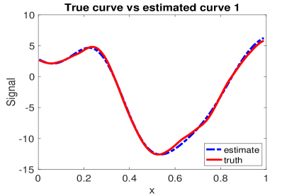
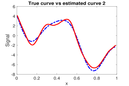
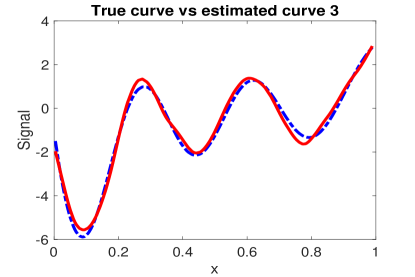
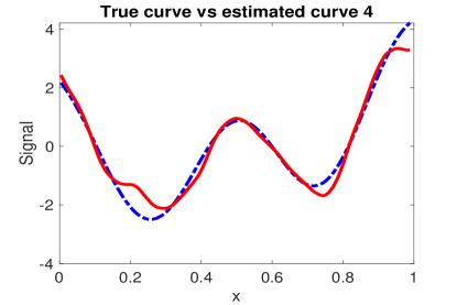
Figure 1: Simulation results: Panels (a)–(d) plot the estimated $\hat{f}_{1}$, $\hat{f}_{2}$, $\hat{f}_{3}$, $\hat{f}_{4}$ from our nonparametric principal subspace regression and their corresponding true functions $f_{1}$, $f_{2}$, $f_{3}$ and $f_{4}$ from a randomly selected Monte Carlo run in the case $(n,p,q)=(256,40,4)$.

We have performed additional simulation studies, where the error $z_{i}$’s are correlated across $1\leq i\leq n$ and the components within each $z_{i}$ are also correlated, reflecting more realistic settings in real applications. The additional simulation results are included in Section 7 of the supplementary file, and indicate that our method still outperforms curve-by-curve nonparametric regression.

3.2 Application to an electroencephalogram study

We apply the proposed method to an electroencephalogram dataset, which is available at https://archive.ics.uci.edu/ml/datasets/EEG+Database. The data were collected by the Neurodynamics Laboratory and contain 122 subjects. Researchers measured the voltage values from 64 electrodes placed on each subject’s scalps sampled at 256 Hz for 1 second. As electroencephalogram data are notoriously noisy while there are known to be strong correlations between different electrodes, the data from each subject may be considered as a sample from model (1). In particular, for each subject, we obtain a data matrix $Y=(y_{1}\ldots y_{n})\in\mathbb{R}^{p\times n}$ with $p=64$ and $n=256$. We fit the nonparametric principal subspace regression to the data matrix obtained from each subject. The average retained dimension selected by the proposed aic among these 122 subjects is $6.959$ with standard error $0.113$. We have plotted the estimates of the first three functional components $f_{1}$, $f_{2}$ and $f_{3}$ from a randomly selected subject in Figure 2 (b)-(d). The curves show clear nonlinear patterns along the covariate time, which can not be captured by either classical factor model, singular value decomposition or multivariate response linear regression.

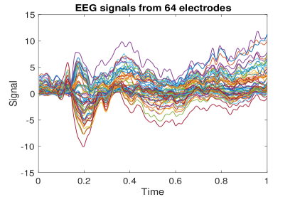
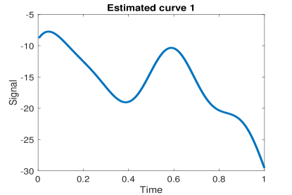
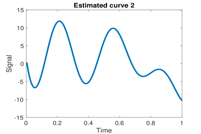
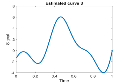
Figure 2: Real data results: Panel (a) plots the electroencephalogram signals detected from 64 electrodes of the scalp of one randomly selected subject. Panels (b)-(d) plot the estimates of the first three functional components $\hat{f}_{1}$, $\hat{f}_{2}$ and $\hat{f}_{3}$ from a randomly selected subject.

To compare the prediction performance, we also fit curve-by-curve nonparametric regression to the signals obtained from each of the $64$ electrodes. For each subject, we randomly reserve $10\%$ of data as the test set: $\mathcal{S}_{\rm{test}}\subseteq\{1,\ldots,256\}$ such that $\left|\mathcal{S}_{\rm{test}}\right|/256\approx 10\%$, while using the rest as the training set, and report the prediction errors $\left|\mathcal{S}_{\rm{test}}\right|^{-1}\left\{\sum_{i\in\mathcal{S}_{\rm{test}}}(\|Y_{i}-\hat{F}(x_{i})\|^{2}/64)\right\}$ for both approaches. The average prediction error for nonparametric principal subspace regression over the 122 subjects is $1.984$ with standard error $0.156$, while that obtained by the curve-by-curve nonparametric regression is $2.344$ with standard error $0.153$.

4 Proofs of Main Theorems

We first introduce the notations used in the rest of this paper, some of the notations have been introduced before. Recall we have proposed a nonparametric model $y_{i}=\sum_{k=1}^{q}f_{k}(x_{i})u_{k}+z_{i}\in\mathbb{R}^{p}$, where $z_{i}=(z_{i1},\ldots,z_{ip})^{\mathrm{\scriptscriptstyle T}}$ follows independent and identically distributed $\mathcal{N}(0,\sigma^{2}I_{p})$. Without loss of generality, in the proof we assume $\sigma^{2}=1$.

Let $Y=(y_{1}\ldots y_{n})\in\mathbb{R}^{p\times n}$ be the response data matrix, $\tilde{F}=(F(x_{1})\ldots F(x_{n}))$ $\in\mathbb{R}^{p\times n}$ and $Z=(z_{1}\ldots z_{n})\in\mathbb{R}^{p\times n}$, one can write $Y\equiv\tilde{F}+Z$. Let $U=(u_{1}\ldots u_{q})\in\mathbb{R}^{p\times q}$, and $\hat{U}=(\hat{u}_{1}\ldots\hat{u}_{q})\in\mathbb{R}^{p\times q}$ the estimate of $U$. Define $\tilde{f}_{k}=(f_{k}(x_{1}),\ldots,f_{k}(x_{n}))^{\mathrm{\scriptscriptstyle T}}\in\mathbb{R}^{n}$ for $1\leq k\leq q$ and $\tilde{f}=(\tilde{f}_{1}\ldots\tilde{f}_{q})^{\mathrm{\scriptscriptstyle T}}\in\mathbb{R}^{q\times n}$ so that $\tilde{F}=U\tilde{f}$. We further define $\tilde{\hat{f}}_{k}=(\hat{f}_{k}(x_{1}),\ldots,\hat{f}_{k}(x_{n}))^{\mathrm{\scriptscriptstyle T}}\in\mathbb{R}^{n}$ for $1\leq k\leq q$ and define $\tilde{\hat{f}}=(\tilde{\hat{f}}_{1}\ldots\tilde{\hat{f}}_{q})^{\mathrm{\scriptscriptstyle T}}\in\mathbb{R}^{q\times n}$ so that we may write $\tilde{\hat{F}}\equiv(\hat{F}(x_{1})\ldots\hat{F}(x_{n}))\in\mathbb{R}^{p\times n}$ as $\tilde{\hat{F}}=\hat{U}\tilde{\hat{f}}$.

Proof of Proposition 2.1.

We may consider $F$ as an operator $F:L^{2}[0,1]^{d}\rightarrow\mathbb{R}^{p}$ mapping $g\in L^{2}[0,1]^{d}$ to

$$Fg=(\langle F_{1},g\rangle_{L^{2}},\dots,\langle F_{p},g\rangle_{L^{2}})\in\mathbb{R}^{p}.$$

In this case we note that under appropriate inner products

$$F=\sum_{k=1}^{p}e_{k}\otimes F_{k}\hskip 5.0pt\text{ and }\hskip 5.0ptF^{*}Fg=\sum_{k=1}^{p}\langle F_{k},g\rangle F_{k}.$$

Thus $F^{*}F$ is of finite rank and hence compact. As it is also symmetric, it has an eigendecomposition

$$F^{*}F=\sum_{k=1}^{\infty}\lambda_{k}^{2}v_{k}\otimes v_{k}$$

with at most $p$ of the $\lambda_{k}\neq 0$ and $v_{k}$ forming an orthonormal basis of $L^{2}[0,1]^{d}$. We order so that the nonzero $\lambda_{k}$ lie in the first $p$ indices and are increasing. Now note that we may write

$$g=\sum_{k=1}^{\infty}\langle g,v_{k}\rangle_{L^{2}}v_{k}.$$

Now, setting $r_{k}=Fv_{k}$ we have that $\langle r_{m},r_{n}\rangle_{L^{2}}=\langle v_{m},F^{*}Fv_{n}\rangle_{L^{2}}=\lambda_{n}^{2}\langle v_{m},v_{n}\rangle_{L^{2}}=\lambda_{n}^{2}\delta_{mn}$. Hence, the $r_{k}$ are orthogonal and at most $p$ of them are nonzero. Setting $\sigma_{k}=1/\lambda_{k}$ for $\lambda_{k}>0$ and $\sigma_{k}=0$ otherwise, we set $u_{k}=\sigma_{k}r_{k}$ and note that since $\sigma_{k}=0$ for the nonzero $r_{k}$, we may write

$$Fg=\sum_{k=1}^{\infty}\langle g,v_{k}\rangle_{L^{2}}Fv_{k}=\sum_{k=1}^{p}\sigma_{k}\langle g,v_{k}\rangle_{L^{2}}u_{k}=\left(\sum_{k=1}^{p}\sigma_{k}u_{k}\otimes v_{k}\right)g.$$

Hence under the appropriate inner products $F$ has the claimed representation. ∎

Proof of Theorem 2.1.

Given the definitions in the paper and at the outset of the supplement, we see that we may write $Y^{o}_{\cdot k}=Y^{\mathrm{\scriptscriptstyle T}}u_{k}$ and $\hat{Y}^{*}_{\cdot k}=Y^{\mathrm{\scriptscriptstyle T}}\hat{u}_{k}$ (both in $\mathbb{R}^{n}$). Direction invariance combined with the assumptions of the theorem guarantee there is a linear smoother $L$, $||L||\leq C$ such that $\tilde{\hat{f}}_{k}=L\hat{Y}^{*}_{\cdot k}$. Consequently $\tilde{\hat{f}}=\hat{U}^{\mathrm{\scriptscriptstyle T}}YL^{\mathrm{\scriptscriptstyle T}}$ and $\tilde{\hat{F}}=\hat{U}\hat{U}^{\mathrm{\scriptscriptstyle T}}YL^{\mathrm{\scriptscriptstyle T}}$ so that, using $\tilde{F}=U\tilde{f}$, we may decompose $\tilde{F}-\tilde{\hat{F}}$ as

$$\tilde{F}-\tilde{\hat{F}}=\underbrace{U\tilde{f}-UU^{\mathrm{\scriptscriptstyle T}}YL^{\mathrm{\scriptscriptstyle T}}}_{\text{I}}+\underbrace{(UU^{\mathrm{\scriptscriptstyle T}}-\hat{U}\hat{U}^{\mathrm{\scriptscriptstyle T}})YL^{\mathrm{\scriptscriptstyle T}}}_{\text{II}}$$

As $U^{\mathrm{\scriptscriptstyle T}}U=I_{q}$, one has

$$\|U\tilde{f}-UU^{\mathrm{\scriptscriptstyle T}}YL^{\mathrm{\scriptscriptstyle T}}\|_{F}^{2} = \mathrm{tr}\{(U\tilde{f}-UU^{\mathrm{\scriptscriptstyle T}}YL^{\mathrm{\scriptscriptstyle T}})^{\mathrm{\scriptscriptstyle T}}(U\tilde{f}-UU^{\mathrm{\scriptscriptstyle T}}YL^{\mathrm{\scriptscriptstyle T}})\}$$

$$= \mathrm{tr}\{(\tilde{f}-U^{\mathrm{\scriptscriptstyle T}}YL^{\mathrm{\scriptscriptstyle T}})^{\mathrm{\scriptscriptstyle T}}(\tilde{f}-U^{\mathrm{\scriptscriptstyle T}}YL^{\mathrm{\scriptscriptstyle T}})\}=\|\tilde{f}-U^{\mathrm{\scriptscriptstyle T}}YL^{\mathrm{\scriptscriptstyle T}}\|_{F}^{2}.$$

Furthermore, the rows of $U^{\mathrm{\scriptscriptstyle T}}YL^{\mathrm{\scriptscriptstyle T}}$ are $\tilde{\hat{f^{o}}}_{k}=LY^{o}_{\cdot k}$. Thus, given the assumptions in Theorem 2.1, we have

$$\frac{1}{n}E(\|\text{I}\|_{F}^{2}) = \frac{1}{n}E(\|\tilde{f}-U^{\mathrm{\scriptscriptstyle T}}YL^{\mathrm{\scriptscriptstyle T}}\|_{F}^{2})=\sum_{k=1}^{q}E(\|f_{k}-\hat{f}^{o}_{k}\|_{n}^{2})$$

$$\leq q\max_{k}E(\|f_{k}-\hat{f}^{o}_{k}\|_{n}^{2})\leq Cqn^{-r}.$$

On the other hand, as $\|L\|\leq C$, one has

$$\|\text{II}\|_{F}^{2} = \|(UU^{\mathrm{\scriptscriptstyle T}}-\hat{U}\hat{U}^{\mathrm{\scriptscriptstyle T}})YL^{\mathrm{\scriptscriptstyle T}}\|_{F}^{2}\leq C\|UU^{\mathrm{\scriptscriptstyle T}}-\hat{U}\hat{U}^{\mathrm{\scriptscriptstyle T}}\|_{F}^{2}\|Y\|^{2}$$

$$\leq qC\|UU^{\mathrm{\scriptscriptstyle T}}-\hat{U}\hat{U}^{\mathrm{\scriptscriptstyle T}}\|^{2}\|Y\|^{2}.$$

Then taking expectations and using that $\|UU^{\mathrm{\scriptscriptstyle T}}-\hat{U}\hat{U}^{\mathrm{\scriptscriptstyle T}}\|\leq 2\|\sin\{\Theta(\hat{U},U)\}\|$ together with an application of Cauchy-Schwarz and lemma 5.1 gives that

$$E(\|\text{II}\|_{F}^{2})\leq Cq\left\{\left(\frac{p}{n}\right)^{2}\wedge 1\right\}^{1/2}\left\{\max(p^{2},n^{2})\right\}^{1/2}\leq Cqp\max\left(1,\frac{p}{n}\right).$$

As $p=o(n)$, applying the triangle inequality to the decomposition of $\|\tilde{F}-\tilde{\hat{F}}\|_{F}^{2}$, taking expectations and combining what has been shown together with the fact that $R_{n}(\hat{F})=E\|\tilde{F}-\tilde{\hat{F}}\|_{F}^{2}/n$ concludes the proof of the theorem. ∎

To prove Theorem 2.2, we need to first bound $E\|\sin\{\Theta(\hat{U},U)\}\|^{4}$. Then one can apply Theorem 2.1 to reach the final conclusion of Theorem 2.2.

Proof of Theorem 2.2.

As noted above it is enough to show that with $\tilde{F}=U\tilde{f}$ and $Y=\tilde{F}+Z$, the left singular vectors of the singular value decomposition of $Y$, $Y=\hat{U}\hat{\Sigma}\hat{V}^{\mathrm{\scriptscriptstyle T}}$, satisfy the bound

$$E[\|\sin\{\Theta(\hat{U},U)\}\|^{4}]\leq C\left(\frac{p}{n}\right)^{2}\wedge 1.$$

As the $\tilde{f}_{k}$’s are not necessarily orthogonal in $\mathbb{R}^{n}$, we need to consider that the singular value decomposition of $\tilde{F}$ is of the form $\tilde{F}=P\Gamma Q^{\mathrm{\scriptscriptstyle T}}$, with $P$ possibly spanning a different subspace from $U$. Let $\mathcal{A}$ be the event given by

$$\mathcal{A}=\Big{\{}\mathrm{span}(P)=\mathrm{span}(U)\Big{\}}.$$

Then Lemma 5.4 shows that $\mathrm{pr}(\mathcal{A})\geq 1-B/n^{2}$. Then given that $\|\sin\{\Theta(P,U)\}\|\leq 1$ for any pair of subspaces and on the event $\mathcal{A}$, $\sin\{\Theta(P,U)\}=0$, it holds that

$$E[\|\sin\{\Theta(P,U)\}\|^{4}] = E[\|\sin\{\Theta(P,U)\}\|^{4}1_{\mathcal{A}}]+E[\|\sin\{\Theta(P,U)\}\|^{4}1_{\mathcal{A}^{c}}]$$

$$\leq \mathrm{pr}(\mathcal{A}^{c})\leq B/n^{2}.$$

Thus we may conclude that

$$E[\|\sin\{\Theta(P,U)\}\|^{4}]\leq C\left(\frac{p}{n}\right)^{2}\wedge 1.$$

By the triangle inequality,

$$\|\sin\{\Theta(\hat{U},U)\}\|^{4} \leq \left[\|\sin\{\Theta(P,U)\}\|+\|\sin\{\Theta(P,\hat{U})\}\|\right]^{4}$$

$$\leq C\left[\|\sin\{\Theta(P,U)\}\|^{4}+\|\sin\{\Theta(P,\hat{U})\}\|^{4}\right].$$

To complete the proof, it suffices to show that $E[\|\sin\{\Theta(P,\hat{U})\}\|^{4}]$ satisfies the bound of the theorem. Now we consider the event $\mathcal{E}$ that the singular values of $\tilde{F}$ scale like $n^{1/2}$,

$$\mathcal{E}=\Big{\{}n^{1/2}c\leq\Gamma_{qq}\leq n^{1/2}C\Big{\}},$$

where $c,C>0$ satisfy $c\leq\min_{k}\|f_{k}\|_{L^{2}}\leq\max_{k}\|f_{k}\|_{L^{2}}\leq C$ and $\Gamma_{qq}$ is the $q$-th element of $\Gamma$. Then Lemma 5.5 implies that $\mathrm{pr}(\mathcal{E})\geq 1-D/n^{2}$. Denote $E\left(\cdot|\mathcal{D}\right)$ the expectation conditioned on design. As $\|\sin\{\Theta(P,\hat{U})\}\|\leq 1$, we may decompose $E\|\sin\{\Theta(P,\hat{U})\}\|^{4}$ as

$$E[\|\sin\{\Theta(P,\hat{U})\}\|^{4}] = E\left(E\left[\left.\|\sin\{\Theta(P,\hat{U})\}\|^{4}\right|\mathcal{D}\right]\right)$$

$$\leq \mathrm{pr}(\mathcal{E}^{c})+E\left(E\left[\left.\|\sin\{\Theta(P,\hat{U})\}\|^{4}\right|\mathcal{D}\right]1_{\mathcal{E}}\right).$$

We extend the proof of theorem 3 in Cai and Zhang, (2018) to bounds for fourth moment of $\|\sin\{\Theta(P,\hat{U})\}\|$ such that

$$E\left[\left.\|\sin\{\Theta(P,\hat{U})\}\|^{4}\right|\mathcal{D}\right]\leq C\left[\frac{p\{\sigma_{q}^{2}(\tilde{F})+n\}}{\sigma_{q}^{4}(\tilde{F})}\right]^{2}\wedge 1.$$

On the event $\mathcal{E}$. By construction, on the event $\mathcal{E}$ we also have that $n^{1/2}c\leq\Gamma_{qq}=\sigma_{q}(F)\leq n^{1/2}C$ and so

$$\frac{p\{\sigma_{q}^{2}(\tilde{F})+n\}}{\sigma_{q}^{4}(\tilde{F})}\leq\frac{p(C+1)n}{c^{2}n^{2}}\leq C\frac{p}{n}.$$

Using the bound on $\mathrm{pr}(\mathcal{E}^{c})$ and piecing together what has been shown concludes the proof of the theorem. ∎

Here we carefully go through the arguments of Theorem 3 in Cai and Zhang, (2018) to guarantee that they hold in our case, using the notation of that paper. As noted in that proof, by symmetry it is enough to extend the method of proof for the right singular vectors and we employ the same concentration results outlined at the outset of the proof. This is because the left singular vectors of $Y$ are just the right singular vectors of $Y^{\mathrm{\scriptscriptstyle T}}$. Thus we can apply the results for the right singular vectors of $Y$ to $Y^{\mathrm{\scriptscriptstyle T}}$ to get bounds for estimation of the left singular vectors of $Y$. Based on the proof we just need to extend the inequality to the case that $\sigma^{2}_{r}(X)\geq C_{\text{gap}}\{(p_{1}p_{2})^{1/2}+p_{2}\}$. Now, under the event $\mathcal{Q}$ given there, the inequality given there implies that

$$\|\sin\Theta(\hat{V},V)\|^{4}\leq C\left\{\frac{\sigma^{2}_{r}(X)+p_{1}}{\sigma^{4}_{r}(X)}\right\}^{2}\|\mathbb{P}_{YV}YV_{\perp}\|^{4},$$

which, in turn, gives that

$$E\left\{\|\sin\Theta(\hat{V},V)\|^{4}\right\}\leq\mathrm{pr}(\mathcal{Q}^{c})+C\left\{\frac{\sigma^{2}_{r}(X)+p_{1}}{\sigma^{4}_{r}(X)}\right\}^{2}E(\|\mathbb{P}_{YU}YU_{\perp}\|^{4}1_{\mathcal{Q}}).$$

In this regime (where $\sigma^{2}_{r}(X)\geq C_{\text{gap}}\{(p_{1}p_{2})^{1/2}+p_{2}\}$) a bound is given for $\mathrm{pr}(\mathcal{Q}^{c})$ of

$$\mathrm{pr}(\mathcal{Q}^{c})\leq\exp\left\{-c\frac{\sigma^{4}_{r}(X)}{\sigma^{2}_{r}(X)+p_{1}}\right\}.$$

When the fraction in the exponent diverges, the exponent tends to zero faster than any polynomial and so we have

$$\mathrm{pr}(\mathcal{Q}^{c})\leq C\left\{\frac{\sigma^{2}_{r}(X)+p_{1}}{\sigma^{4}_{r}(X)}\right\}^{2}\leq C\left\{\frac{p_{2}(\sigma^{2}_{r}(X)+p_{1})}{\sigma^{4}_{r}(X)}\right\}^{2}.$$

Considering what happens if the exponent is not diverging, we see that this holds in either case. Thus for the desired extension, it remains to show that $E(\|\mathbb{P}_{YU}YU_{\perp}\|^{4}1_{\mathcal{Q}})$ $\leq Cp_{2}^{2}$. As in the proof, we let $T=\|\mathbb{P}_{YU}YU_{\perp}\|$ and note that (using the concentration bounds employed in the theorem)

$$E(T^{4}1_{\mathcal{Q}}) \leq E\{T^{4}1_{(T^{2}\leq\sigma_{r}^{2}(x)+p_{1})}\}=\int_{0}^{\infty}\mathrm{pr}\left\{T^{4}1_{(T^{2}\leq\sigma_{r}^{2}(x)+p_{1})}>t\right\}dt$$

$$\leq \delta p_{2}^{2}+\int_{\delta p_{2}^{2}}^{\{\sigma_{r}^{2}(x)+p_{1}\}^{2}}\mathrm{pr}\left(T>t^{1/4}\right)dt$$

$$\leq \delta p_{2}^{2}+C\int_{\delta p_{2}^{2}}^{\{\sigma_{r}^{2}(x)+p_{1}\}^{2}}\left(\exp(Cp_{2}-ct)+\exp[-c\{\sigma_{r}^{2}(X)+p_{1}\}]\right)dt$$

$$\leq \delta p_{2}^{2}+C\{\sigma_{r}^{2}(x)+p_{1}\}^{2}\exp[-c\{\sigma_{r}^{2}(X)+p_{1}\}]+$$

$$+C\exp(Cp_{2})\cdot\exp(-c\delta p_{2})/c.$$

From this, we see that choosing $\delta$ large enough we may guarantee that $E(T^{4}1_{\mathcal{Q}})\leq Cp_{2}^{2}$, which is what we wanted. This is the final piece needed in showing that the form of the bound we wanted holds for the fourth moment.

5 Relevant Lemmas for Main Theorems

We introduce the auxiliary lemmas for main theorems in Section 4, the proofs of which are deferred to the Section 9 of the supplementary file.

The next two results bound fourth moments of $\|Y\|$ and $\sin\{\Theta(\tilde{U},U)\}$. In the results that follow, $Z\in\mathbb{R}^{p\times n}$ is composed of independent and identically distributed $\mathcal{N}(0,1)$ entries. The first main lemma is as follows

Lemma 5.1.

With $Y=\tilde{F}+Z\in\mathbb{R}^{p\times n}$ denoting the data matrix and $\|Y\|=\max_{i}\sigma_{i}(Y)$ the operator norm, or maximum singular value, of $Y$ we have that

$$E(\|Y\|^{4})\leq C\max(p^{2},n^{2})$$

holds when $\max_{k}\|f_{k}\|_{\infty}\leq B$.

Next, we show the lemma needed in the proof of Lemma 5.1.

Lemma 5.2.

If $X\geq 0$ is a positive random variable and for $a,b>0$ we have $\mathrm{pr}(X>a+bt)\leq 2\exp(-t^{2})$ for all $t\geq 0$ then it follows that $E(X^{4})\leq C\max(a^{4},b^{4})$.

The next lemma quantifies the discrepancy between $\langle\cdot,\cdot\rangle_{n}$ and $\langle\cdot,\cdot\rangle_{L^{2}}$. These are crucial to the proofs of Lemmas 5.4 and 5.5 which, in turn are crucial to the proofs of the main theorems of the paper.

Lemma 5.3.

Suppose that $x_{i}\sim\mathcal{U}[0,1]^{d}$ are independently drawn from the uniform distribution on the unit cube in $\mathbb{R}^{d}$ and $f_{1},\dots,f_{q}$ are bounded and orthogonal in $L^{2}[0,1]^{d}$, satisfying $\max_{i\leq q}\|f_{i}\|_{\infty}\leq B$. Then,

$$\mathrm{pr}(\max_{i,j}|\langle f_{i},f_{j}\rangle_{n}-\langle f_{i},f_{j}\rangle|>2\delta B^{2})\leq q(q+1)\exp\left(-\frac{n\delta^{2}}{2}\right)$$

and so, with probability $\geq 1-q(q+1)/n^{2}$,

$$\max_{i,j}|\langle f_{i},f_{j}\rangle_{n}-\langle f_{i},f_{j}\rangle|\leq 4B^{2}\left(\frac{\log n}{n}\right)^{1/2}.$$

Let $\tilde{F}=U\tilde{f}\in\mathbb{R}^{p\times n}$, as defined above, represent the sampled version of the singular value decomposition representation of the target

$$F=\sum_{k=1}^{q}u_{k}\otimes f_{k}=\sum_{k=1}^{q}\sigma_{k}u_{k}\otimes v_{k},$$

where we have set $\sigma_{k}=\|f_{k}\|_{L^{2}}$ and $v_{k}=f_{k}/\|f_{k}\|_{L^{2}}$. Further, we let $\tilde{F}=P\Gamma Q^{\mathrm{\scriptscriptstyle T}}$ denote the singular value decomposition of $\tilde{F}$. Recall that the matrix $\tilde{f}\in\mathbb{R}^{q\times n}$ collects the sampled values of the $f_{k}$ in its rows.

Due to sampling, it is not clear whether $\tilde{F}$ is a close approximation to $F$ in either of the following senses:

1, The matrix $\tilde{F}$ provides a close approximation to the singular vectors we wish to estimate in that the span’s are the same, i.e. $\mathrm{span}(\tilde{F})=\mathrm{span}(P)=\mathrm{span}(U)$. This in turn guarantees that $\sin\Theta(P,U)=0$.

2, The matrix $\tilde{F}$ is “large” enough to separate signal from noise in estimating the $U$.

The following lemmas resolve these issues and are central to the proof of Theorem 2.2.

Lemma 5.4.

We eventually have $\mathrm{span}(\tilde{F})=\mathrm{span}(U)$ with probability greater than or equal to $1-B/n^{2}$ for some fixed $B\geq 0$. As $\mathrm{span}(\tilde{F})=\mathrm{span}(P)$, with $P$ from the singular value decomposition of $\tilde{F}=P\Gamma Q^{\mathrm{\scriptscriptstyle T}}$, this guarantees $\mathrm{span}(P)=\mathrm{span}(U)$ and hence $\sin\Theta(P,U)=0$.

Lemma 5.5.

Let $\tilde{F}$ represent the sampled version of the singular value decomposition representation of the target

$$F=\sum_{k=1}^{q}u_{k}\otimes f_{k}=\sum_{k=1}^{q}\sigma_{k}u_{k}\otimes v_{k},$$

where $\otimes$ is the Kronecker product. Under the conditions of Theorem 2.2, where we have set $\sigma_{k}=\|f_{k}\|_{L^{2}}$ and $v_{k}=f_{k}/\|f_{k}\|_{L^{2}}$, if $\gamma$ is one of the top $q$ singular value of $\tilde{F}$, $\gamma$ satisfies

$$\min_{i\leq q}|\gamma-n^{1/2}\sigma_{i}|\leq Cq^{1/2}\left(n\log n\right)^{1/4}$$

with probability at least $1-B/n^{2}$ for some $B\geq 0$. In particular, it follows that if $c\leq\min_{k}\sigma_{k}\leq\max_{k}\sigma_{k}\leq C$ then, with possibly adjusted constants, $\gamma$ satisfies

$$n^{1/2}c\leq\gamma\leq n^{1/2}C$$

with probability at least $1-B/n^{2}$, for some $B\geq 0$ and large enough $n$.

For the proof of Lemma 5.5, we need a well known perturbation result for matrices (Weyl,, 1912), which will ease the proof of this result considerably.

Lemma 5.6.

(Weyl) Let the eigenvalues of real symmetric matrices $A$ and $A+E$ be $\lambda_{1}\geq\lambda_{2}\geq\dots\geq\lambda_{n}\geq 0$ and $\tilde{\lambda}_{1}\geq\tilde{\lambda}_{2}\geq\dots\geq\tilde{\lambda}_{n}\geq 0$ respectively. Then $\max_{i}|\lambda_{i}-\tilde{\lambda}_{i}|\leq\|E\|_{2}$.

6 Details on Examples and Attained Rates

We introduce the lemmas and theorems for examples in the Section 2.3, the proofs of which are deferred to the Section 9 of the supplementary file.

6.1 Local Polynomial Regression

For this section, the smoothness class of primary concern is the Hölder class, $\Sigma(\beta,L)$. For any real number $x$, let $\lfloor x\rfloor$ represent the largest integer strictly less than $x$. Then $\Sigma(\beta,L)$ consists of all functions $f$ which are $l=\lfloor\beta\rfloor$ times differentiable and whose $l$th derivative $f^{(l)}$ satisfies

$$|f^{(l)}(x)-f^{(l)}(y)|\leq L|x-y|^{\beta-l},$$

for all $x,y$ in the domain of interest.

It is well known that in the fixed design case, where we roughly have $x_{i}=i/n$, if the kernel and bandwidth are properly chosen, then local polynomial smoothing gives an estimator $\hat{f}$ of $f$ from the data

$$y_{i}=f(x_{i})+z_{i},$$

which satisfies

$$E_{f}\|\hat{f}_{n}-f\|_{n}^{2}\leq Cn^{-2\beta/(1+2\beta)}.$$

Furthermore, this rate is minimax optimal. For proof and in depth setup, see proposition 1.13 and theorem 1.6 in Tsybakov, (2008). In the random design case, there don’t seem to be any results on convergence in the metric we want, namely $E_{f}\|\cdot\|_{n}^{2}$.

One remedy to this is to adopt a similar approach to that in Cai and Brown, (1999), and slightly modify the local polynomial regression strategy. To this end, let $0\leq x_{(1)}\leq\dots\leq x_{(n)}\leq 1$ represent the order statistics of the uniform design and relabel the $y_{i}$’s and $z_{i}^{\prime}s$ according to these so that $y_{i}=f(x_{(i)})+z_{i}$ generate the observations. In the recovery procedure, we pretend that $x_{(i)}$ is $\delta_{i}=Ex_{(i)}=i/(n+1)$ so that we perform local polynomial regression as if the observations were $\left(\delta_{i},y_{i}\right)$ for $i=1,\dots,n$. That is, with $K$ being a kernel satisfying the right conditions and

$$U(u)=\left(1,u,\frac{u^{2}}{2},\dots,\frac{u^{l}}{l!}\right)^{\mathrm{\scriptscriptstyle T}},$$

we form the estimate

$$\hat{\theta}(x)=\arg\min_{\theta}\sum_{i=1}^{n}\left\{y_{i}-\theta^{\mathrm{\scriptscriptstyle T}}U\left(\frac{\delta_{i}-x}{h}\right)\right\}^{2}K\left(\frac{\delta_{i}-x}{h}\right)$$

and we estimate $f$ by

$$\hat{f}(x)=U(0)^{\mathrm{\scriptscriptstyle T}}\hat{\theta}(x).$$ (4)

Then for a given $x$, $\hat{f}(x)$ is linear in the $y_{i}$ in that one may show

$$\hat{f}(x)=\sum_{i=1}^{n}W_{n,i}(x)y_{i},$$

as for a standard local polynomial estimator. Further, the $W_{n,i}(x)$ are now completely deterministic, satisfying all of the properties derived in Tsybakov, (2008). We can then show that this estimator achieves the rate we want in the metric we need it to, as the following theorem guarantees.

Theorem 6.1.

(Local Polynomial Smoothing) Suppose that $f$ belongs to the Hölder class $\Sigma(\beta,L)$, the design is uniform random and the kernel $K$ satisfies the properties outlined in Tsybakov, (2008). Then we may be assured that $\hat{f}$ outlined above satisfies

$$E_{f}\|\hat{f}-f\|_{n}^{2}\leq Cn^{-2\beta/(1+2\beta)}.$$

For local polynomial smoothing, we have $\|L\|\leq C$. This follows from a result for bounds of eigenvalues of matrices. Let $A=(a_{kl})_{k,l=1}^{n}$ be an $n\times n$ matrix and set

$$R_{k}=\sum_{l}|a_{kl}|\hskip 5.0pt\text{ and }\hskip 5.0ptC_{l}=\sum_{k}|a_{kl}|.$$

Then one can show that the eigenvalues of $A$, $\mu(A)$, are bounded by

$$\mu(A)\leq\min\left(\max_{k}R_{k},\max_{l}C_{l}\right)\leq\max_{k}R_{k}.$$

In the case of local polynomial smoothing, the $L$ satisfies $L_{ij}=W_{n,j}(x_{i})$ and from Tsybakov, (2008) we know that

$$R_{i}=\sum_{j}|L_{ij}|=\sum_{j}|W_{n,j}(x_{i})|\leq C.$$

Thus we have that $\mu(L)\leq C$ and thus $\|L\|\leq C$.

6.2 Truncated Series Estimation

For extensive setup and analysis of fixed design for Fourier basis and Sobolev smoothness, see Tsybakov, (2008). Here the smoothness class of interest is the Sobolev class of periodic functions of integer smoothness $\beta$, denoted by $W^{p}(\beta,L)$. To define this class of functions, we start with the Sobolev class $W(\beta,L)$ defined by

$$W(\beta,L)=\left\{f\in L^{2}[0,1]:f^{(\beta-1)}\in\mathcal{C}[0,1]\text{ and }\int_{0}^{1}(f^{(\beta)})^{2}\leq L\right\},$$

where $\mathcal{C}[0,1]$ is the collection of absolutely continuous functions on $[0,1]$. The function class of interest, $W^{p}(\beta,L)$, is then defined by

$$W^{p}(\beta,L)=\left\{f\in W(\beta,L):f^{(j)}(0)=f^{(j)}(1)\text{ for }j=0,1,\dots,\beta-1\right\}.$$

Fix the Fourier basis, where $\varphi_{1}=1$ and $\varphi_{2k}=2^{1/2}\cos(2\pi x)$, $\varphi_{2k+1}={2}^{1/2}\sin(2\pi x)$ for $k\geq 1$. It is known that every $f\in W^{p}(\beta,L)$ has a Fourier expansion of the form

$$f=\sum_{k=1}^{\infty}f_{k}\varphi_{k}$$

and that the coefficients of all $f\in W^{p}(\beta,L)$ lie in an ellipsoid of the form

$$Q(\beta,C)=\left\{(c_{k})\in\ell_{2}:\sum_{k\geq 1}a_{k}^{2}c_{k}^{2}\leq C\right\},$$

where the $a_{k}\sim k^{\beta}$.

Now let $\{\varphi_{k}\}_{k\geq 1}$ be an orthonormal basis of $L^{2}[0,1]$, $x_{i}\stackrel{{\scriptstyle i.i.d.}}{{\sim}}U[0,1]$ represent a uniform random design on $[0,1]$ and set

$$\hat{c}_{k}=\frac{1}{n}\sum_{i=1}^{n}y_{i}\varphi_{k}(x_{i})\hskip 5.0pt\text{ and }\hskip 5.0pt\hat{f}_{n,K}=\sum_{k=1}^{K}\hat{c}_{k}\varphi_{k}.$$

For analysis of the estimator $\hat{f}_{n,K}$, we set

$$\overline{c}_{k}=\frac{1}{n}\sum_{i=1}^{n}f(x_{i})\varphi_{k}(x_{i})$$

and notice that we have $E_{f,\mathbb{X}}(\hat{c}_{k})=\overline{c}_{k}$ and $E_{f}(\overline{c}_{k})=E_{f}(\hat{c}_{k})=c_{k}.$ Setting $f_{K}=\sum_{k>K}c_{k}\varphi_{k}$, we may establish the following theorem

Theorem 6.2.

(Oracle inequality for truncated series estimation) The estimator $\hat{f}_{n,K}$ defined above satisfies the risk bound

$$E_{f}(\|f-\hat{f}_{n,K}\|_{n}^{2})\leq 2\frac{(1+K/n)(1+\|f\|_{L^{2}}^{2})K}{n}+2E_{f}(\|f_{K}\|_{n}^{2}).$$

Now assumptions on the decay of the $c_{k}$ will provide bounds on the error of the estimator. For instance, assuming that $f\in W^{p}(\beta,L)$ implies that $(c_{k})\in Q(\beta,C)$, as above. This implies that

$$E_{f}(\|f_{K}\|_{n}^{2}) = \|f_{K}\|_{L^{2}}^{2}=\sum_{k>K}c_{k}^{2}$$

$$= \sum_{k>K}a_{k}^{-2}a_{k}^{2}c_{k}^{2}\leq a_{K}^{-2}\sum_{k>K}a_{k}^{2}c_{k}^{2}\leq Ca_{K}^{-2}\leq CK^{-2\beta}.$$

Employing the Theorem 6.2, this gives that

$$E_{f}(\|f-\hat{f}_{n,K}\|_{n}^{2})\lesssim\frac{K}{n}+K^{-2\beta}.$$

Choosing $K\sim n^{1/(1+2\beta)}$ gives $E_{f}(\|f-\hat{f}_{n,K}\|_{n}^{2})\lesssim n^{-2\beta/(1+2\beta)}$ which is the known minimax rate for these classes.

For projection estimation, we have $\|L\|\leq C$. This follows since the least squares estimator is a projection estimator and hence all eigenvalues are less or equal to $1$.

6.3 Reproducing Kernel Hilbert space Regression

Let $K$ be a positive semidefinite kernel function $[0,1]^{2}$ and $\mathcal{H}=\mathcal{H}(K)$ the associated reproducing kernel Hilbert space on $[0,1]$ with norm $\|\cdot\|_{\mathcal{H}}$. We are interested in the performance of penalized estimation strategies

$$\hat{f}_{n,K}=\arg\min_{g\in\mathcal{H}}\left\{\frac{1}{2}\|y-g\|_{n}^{2}+\lambda_{n}\|g\|_{\mathcal{H}}^{2}\right\},$$

which, by the representer theorem, takes the form of linear smoothers. In particular, if we set $K=(K(x_{i},x_{j})/n)_{i,j=1}^{n}$ then we find that

$$\hat{f}_{n,K}=n^{-1/2}\sum_{i=1}^{n}\hat{\alpha}_{i}K(\cdot,x_{i})\hskip 5.0pt\text{ where }\hskip 5.0pt\hat{\alpha}=n^{-1/2}(K+\lambda I)^{-1}y$$

so that

$$(\hat{f}_{n,K}(x_{1}),\dots,\hat{f}_{n,K}(x_{1}))^{\mathrm{\scriptscriptstyle T}}=K(K+\lambda I)^{-1}y=Ly$$

is linear in the data, with $L=K(K+\lambda I)^{-1}$; here we naturally have $\|L\|\leq 1$, as can be seen expanding $L$ in the eigendecomposition of $K$. See chapter 12 of Wainwright, (2019) for details and more extensive development.

In analyzing the estimator $\hat{f}_{n,K}$, the difference symmetrized space, $\partial\mathcal{H}$, defined by

$$\partial\mathcal{H}=\mathcal{H}-\mathcal{H}=\left\{\left.g-h\right|g,h\in\mathcal{H}\right\},$$

turns out to be an important quantity. For $\delta>0$ we define the localized sets

$$\partial\mathcal{H}_{n}(\delta)=\left.\left\{g\in\partial\mathcal{H}\right|\|g\|_{\mathcal{H}}\leq 3,\|g\|_{n}\leq\delta\right\},$$

consisting of functions in $\mathcal{H}$ with small empirical norm. The localized gaussian complexity, $\mathcal{G}_{n}(\delta)$, associated with $\mathcal{H}$ and a given set of sampling points $\mathbb{X}_{n}=\{x_{1},\dots,x_{n}\}$, is defined by

$$\mathcal{G}_{n}(\delta)=E_{w}\left\{\left.\sup_{g\in\partial\mathcal{H}_{n}(\delta)}\left|\langle w,g\rangle_{n}\right|\right|\mathbb{X}_{n}\right\},$$

where $w\sim N_{n}(0,I_{n})$, and can be used to control the error of the estimation procedure $\hat{f}_{n,K}$. For this setup, the gaussian complexity is known to satisfy the bound

$$\mathcal{G}_{n}(\delta)\leq\mathcal{G}^{K}_{n}(\delta)=\left\{\frac{2}{n}\sum_{k=1}^{n}\min(\delta^{2},\hat{\mu}_{j})\right\}^{1/2},$$

with $\hat{\mu}_{j}$ being the eigenvalues of the empirical kernel matrix $K$. Now with $\delta_{n}>0$ being a positive solution of $2\mathcal{G}_{n}(\delta)\leq R\delta^{2}$, and $\lambda$ chosen from the range $[2\delta_{n}^{2},C\delta_{n}^{2}]$, $C>2$, as shown in chapter 13 of Wainwright, (2019), the estimator $\hat{f}_{n,K}$ satisfies the the oracle inequality

$$E(\|f-\hat{f}_{n,K}\|_{n}^{2}\left|\mathbb{X}_{n}\right.)\leq C\left\{\inf_{\|g\|_{\mathcal{H}}\leq R}\|f-g\|_{n}^{2}+R^{2}\delta_{n}^{2}\right\}.$$

Thus if we choose $\delta_{n}>0$ being the smallest number satisfying $2\mathcal{G}^{K}_{n}(\delta)\leq R\delta^{2}$ and $f\in\mathcal{H}$ with $\|f\|_{\mathcal{H}}\leq R$, then we have that $E(\|f-\hat{f}_{n,K}\|_{n}^{2}\left|\mathbb{X}_{n}\right.)\leq C\delta_{n}^{2}$ and so $E(\|f-\hat{f}_{n,K}\|_{n}^{2})\leq CE_{\mathbb{X}_{n}}\delta_{n}^{2}$, which we will proceed to bound for some concrete examples, using known eigenvalue decay of some common operators.

6.3.1 Oracle inequality applied to random design

As per the program outlined above, the goal is to bound the estimation error $E(\|f-\hat{f}_{n,K}\|_{n}^{2})$ by bounding $E_{\mathbb{X}_{n}}\delta_{n}^{2}$ for various $\mathcal{H}=\mathcal{H}(K)$. This is done by relating the eigenvalues $\hat{\mu}_{j}$ of the empirical kernel matrix $K$ to those $\mu_{j}$ of the underlying kernel $K$, viewed as an integral operator; the order of these eigenvalues are known for various important $\mathcal{H}=\mathcal{H}(K)$, which allows us to bound the rate of estimation. In particular, if we know the order of the $\mu_{j}$, we can calculate the minimum positive solution to the population complexity equation $2\overline{\mathcal{G}}_{n}^{K}(\delta)\leq R\delta^{2}$, say $\gamma_{n}$, where

$$\overline{\mathcal{G}}_{n}^{K}(\delta)=\left\{\frac{2}{n}\sum_{j=1}^{\infty}\min(\mu_{j},\delta^{2})\right\}^{1/2}.$$

If the $\hat{\mu}_{j}$ are not overly different from the $\mu_{j}$, the hope is that $\delta_{n}$ and $\gamma_{n}$ are not overly different.

First we need a couple of new definitions. We need the notion of local Rademacher complexity, $\mathcal{R}_{n}(\delta)$, of a function class defined by

$$\mathcal{R}_{n}(\delta)=E_{b}\left\{\left.\sup_{g\in\partial\mathcal{H}_{n}(\delta)}\left|\langle b,g\rangle_{n}\right|\right|\mathbb{X}_{n}\right\},$$

where $b\in\{-1,1\}^{n}$ is a collection of independent Bernoulli variables. As with the local Gaussian complexity, $\mathcal{G}_{n}(\delta)$, this quantity is random, depending on the design $\mathbb{X}_{n}$. Similarly, we may define the corresponding population quantities $\overline{\mathcal{R}}_{n}(\delta)$ and $\overline{\mathcal{G}}_{n}(\delta)$

$$\overline{\mathcal{R}}_{n}(\delta)=E_{b,\mathbb{X}_{n}}\left\{\sup_{g\in\partial\mathcal{H}(\delta)}\langle b,g\rangle_{n}\right\}\hskip 5.0pt\text{ and }\hskip 5.0pt\overline{\mathcal{G}}_{n}(\delta)=E_{w,\mathbb{X}_{n}}\left\{\sup_{g\in\partial\mathcal{H}(\delta)}\langle w,g\rangle_{n}\right\},$$

which average over design and take $\sup$’s over $\mathcal{H}(\delta)$. It is known that $\overline{\mathcal{G}}_{n}^{K}(\eta)$ is an upper bound for the corresponding population quantities so that $\overline{\mathcal{G}}_{n}(\delta),\overline{\mathcal{R}}_{n}(\delta)\leq\overline{\mathcal{G}}_{n}^{K}(\delta)$, which will be crucial to what follows. As above, we let $\gamma_{n}$ be the smallest positive solution of $\mathcal{G}_{n}^{K}(\delta)\leq\delta^{2}$ and notice that by the bound above, we know that $\xi_{n}$ dominates the smallest positive solutions to $\overline{\mathcal{G}}_{n}(\delta),\overline{\mathcal{R}}_{n}(\delta)\leq\delta^{2}$. As $g\in\mathcal{H}(\delta),\mathcal{H}_{n}(\delta)$ implies $-g\in\mathcal{H}(\delta),\mathcal{H}_{n}(\delta)$, it follows that the absolute value in the definition of $\mathcal{G}_{n}(\delta)$ is redundant so that

$$\mathcal{G}_{n}(\delta)=E_{w}\left\{\left.\sup_{g\in\partial\mathcal{H}_{n}(\delta)}\langle w,g\rangle_{n}\right|\mathbb{X}_{n}\right\}.$$

The same observation can be made about the local Rademacher complexity. This eases the development of concentration inequalities for these quantities in the development that follows.

Our aim is to relate the solution of the empirical gaussian complexity to the solution to the population gaussian complexity, $\overline{\mathcal{G}}_{n}(\delta)$, which we can calculate a bound for (via $\mathcal{G}_{n}^{K}(\delta)$),

$$\overline{\mathcal{G}}_{n}(\delta)=E_{x,g}\sup_{f\in\partial\mathcal{H}(\delta)}\langle g,f\rangle_{n}.$$

The proof can be divided into two steps. We begin by introducing another version of the empirical complexity

$$\widehat{\mathcal{G}}_{n}(\delta)=E_{g}\left\{\sup_{f\in\partial\mathcal{H}(\delta)}\langle g,f\rangle_{n}\right\}\hskip 5.0pt\text{ where }\hskip 5.0pt\partial\mathcal{H}(\delta)=\left.\left\{g\in\partial\mathcal{H}\right|\|g\|_{\mathcal{H}}\leq 3,\|g\|_{2}\leq\delta\right\},$$

which is random in the design. We show that this is a self-bounding function and that it concentrates swiftly at its expectation, $\overline{\mathcal{G}}_{n}(\delta)=E_{x}\left\{\widehat{\mathcal{G}}_{n}(\delta)\right\}$. At the same time, we show that on sets of high probability $\mathcal{G}_{n}(\delta)\approx\widehat{\mathcal{G}}_{n}(\delta)$. This allows us to show that the empirical $\delta_{n}$ is close to the population $\overline{\delta}_{n}$, for which we can calculate a bound, in probability and expectation.

In this direction, we develop a crucial lemma. First, with $\gamma_{n}$ as above and for $\lambda\geq 1$, we define two sets $\mathcal{E}_{0}(\lambda)$ and $\mathcal{E}_{1}(\lambda)$ by:

$$\mathcal{E}_{0}(\lambda) = \left\{{x}\left|\sup_{f\in\mathcal{F}}\frac{\left|\|f\|_{n}^{2}-\|f\|_{2}^{2}\right|}{\|f\|_{2}^{2}+\lambda^{2}\gamma_{n}^{2}}\leq\frac{1}{2}\right.\right\}$$

$$\hskip 5.0pt\text{ and }\hskip 5.0pt\mathcal{E}_{1}(\lambda) = \left\{{x}\left||\widehat{\mathcal{G}}_{n}(\lambda\gamma_{n})-\overline{\mathcal{G}}_{n}(\lambda\gamma_{n})|\leq\lambda\gamma_{n}^{2}\right.\right\}.$$

Controlling these sets allows us to quantify how close $\mathcal{G}_{n}(\delta)$ is to $\widehat{\mathcal{G}}_{n}(\delta)$ and how close $\widehat{\mathcal{G}}_{n}(\delta)$ is to $\overline{\mathcal{G}}_{n}(\delta)$. For this purpose, we have the following lemma.

Lemma 6.1.

Assume that $K$ is a bounded kernel, so that point evaluations are bounded. Then with $C$ representing possibly different constants at each occurrence, we have that

$$\mathrm{pr}\left\{\mathcal{E}_{0}(\lambda)\right\}\geq 1-C\exp(-Cn\gamma_{n}^{2}\lambda^{2})\hskip 5.0pt,\quad\hskip 5.0pt\mathrm{pr}\left\{\mathcal{E}_{1}(\lambda)\right\}\geq 1-C\exp(-Cn\gamma_{n}^{2}\lambda).$$

Note that on $\mathcal{E}_{0}(\lambda)\cup\mathcal{E}_{1}(\lambda)$, inclusion in $\mathcal{E}_{0}(\lambda)$ guarantees that $\|f\|_{n}\leq 2\|f\|_{2}+\lambda\gamma_{n}$ and $\|f\|_{2}\leq 2\|f\|_{n}+\lambda\gamma_{n}.$ This in turn ensures that

$$\mathcal{G}_{n}(\delta)\leq\widehat{\mathcal{G}}_{n}(2\delta+\lambda\gamma_{n})\hskip 5.0pt\text{ and }\hskip 5.0pt\widehat{\mathcal{G}}_{n}(\delta)\leq\mathcal{G}_{n}(2\delta+\lambda\gamma_{n}).$$

In particular, taking $\delta=\lambda\gamma_{n}$ gives $\mathcal{G}_{n}(\lambda\gamma_{n})\leq\widehat{\mathcal{G}}_{n}(3\lambda\gamma_{n})$. At the same time, inclusion in $\mathcal{E}_{1}(\lambda)$ guarantees that

$$\widehat{\mathcal{G}}_{n}(\lambda\gamma_{n})\leq\overline{\mathcal{G}}_{n}(\lambda\gamma_{n})+\lambda\gamma_{n}^{2},$$

while the fact that $\gamma_{n}$ dominates the smallest positive solution of $\overline{\mathcal{G}}_{n}(\delta)\leq\delta^{2}$ together with the non-increasing property of $\overline{\mathcal{G}}_{n}(\delta)/\delta$ guarantee that for $\lambda\geq 1$, $\gamma_{n}\geq\overline{\mathcal{G}}_{n}(\gamma_{n})/\gamma_{n}\geq\overline{\mathcal{G}}_{n}(\lambda\gamma_{n})/\lambda\gamma_{n}$ and so $\overline{\mathcal{G}}_{n}(\lambda\gamma_{n})\leq\lambda\gamma_{n}^{2}$. Piecing things together, this guarantees that on $\mathcal{E}_{0}(\lambda)\cup\mathcal{E}_{1}(\lambda)$ we have that $6\lambda\gamma_{n}^{2}=3\lambda\gamma_{n}^{2}+3\lambda\gamma_{n}^{2}\geq\overline{\mathcal{G}}_{n}(3\lambda\gamma_{n})+3\lambda\gamma_{n}^{2}\geq\widehat{\mathcal{G}}_{n}(3\lambda\gamma_{n})\geq\mathcal{G}(\lambda\gamma_{n})$ Thus for $\lambda\geq 6$, on $\mathcal{E}_{0}(\lambda)\cup\mathcal{E}_{1}(\lambda)$ we have that $\mathcal{G}_{n}(\lambda\gamma_{n})\leq 6\lambda\gamma_{n}^{2}\leq(\lambda\gamma_{n})^{2}$ so that, with $\delta_{n}$ being the smallest positive solution of $\mathcal{G}_{n}(\delta)\leq\delta^{2}$ we have $\delta_{n}\leq\lambda\gamma_{n}$ and hence $\mathcal{E}_{0}(\lambda)\cup\mathcal{E}_{1}(\lambda)\subseteq\{\delta_{n}\leq\lambda\gamma_{n}\}.$ In particular, applying Lemma 6.1, we have that for $\lambda\geq 6$,

$$\mathrm{pr}(\delta_{n}>\lambda\gamma_{n}) \leq \mathrm{pr}\{\mathcal{E}^{c}_{0}(\lambda)\}+\mathrm{pr}\{\mathcal{E}^{c}_{1}(\lambda)\}$$

$$\leq C\exp(-Cn\gamma_{n}^{2}\lambda^{2})+C\exp(-Cn\gamma_{n}^{2}\lambda)$$

$$\leq C\exp(-Cn\gamma_{n}^{2}\lambda).$$

This provides the concentration of measure result we need to bound the expectation $E_{\mathbb{X}_{n}}(\delta_{n}^{2})$ and cap the rate of the kernel estimation method. Thus we prove the following lemma.

Lemma 6.2.

Let $K$ be a bounded kernel, $\delta_{n}$ be the smallest positive solution to the empirical Gaussian complexity $2\mathcal{G}_{n}(\delta)\leq\delta^{2}$ and $\gamma_{n}$ the smallest solution to $2\overline{\mathcal{G}}^{K}_{n}(\delta)\leq\delta^{2}$. Then, for $C$ possibly changing at each occurrence and $\lambda\geq 6$, we have that

$$\mathrm{pr}(\delta_{n}>\lambda\gamma_{n})\leq C\exp(-Cn\gamma_{n}^{2}\lambda).$$

Consequently, provided $n\gamma_{n}^{2}=O(1)$, it follows that $E_{\mathbb{X}_{n}}\left(\delta_{n}^{2}\right)\leq C\gamma_{n}^{2}$.

Combining what has been shown gives the following theorem characterizing rate for convergence of reproducing kernel Hilbert space based methods in the case of random design.

Theorem 6.3.

Suppose that $K$ is a bounded kernel and $\gamma_{n}$ is the smallest solution to $2\overline{\mathcal{G}}^{K}_{n}(\delta)\leq\delta^{2}$. Then it follows from the work done above that the reproducing kernel Hilbert space based procedure outlined in the intro to this section satisfies the oracle inequality

$$E\left(\|f-\hat{f}_{n,K}\|_{n}^{2}\right)\leq C\left(\gamma_{n}^{2}+E_{\mathbb{X}_{n}}\inf_{\|g\|_{\mathcal{H}}\leq R}\|f-g\|_{n}^{2}\right).$$

Consequently, if $f\in\mathcal{H}$ and satisfies $\|f\|_{\mathcal{H}}\leq R$ we have $E(\|f-\hat{f}_{n,K}\|_{n}^{2})\leq C\gamma_{n}^{2}.$ If the eigenvalues of $K$ decay like $\lambda_{i}\sim i^{-\alpha}$, this means that $E(\|f-\hat{f}_{n,K}\|_{n}^{2})\leq Cn^{-\alpha/(\alpha+1)}$.

Supplement to “Nonparametric principal subspace regression”

This supplementary file includes additional simulation results, proofs of lemmas and convergence rates for the examples in Section 2.3.

7 Additional Simulation Results

In this section, we perform additional simulation studies, where the error $z_{i}$’s are assumed to be correlated across $1\leq i\leq n$ and the components within each $z_{i}$ are also correlated. Let $Z=(z_{1}\ldots z_{n})$ denote a $p\times n$ random error matrix with entries $z_{ji}$, $1\leq j\leq p$ and $1\leq i\leq n$, and $\mathrm{vec}$ denote the vectorization operator that stacks the columns of a matrix into a vector. We set $\mathrm{vec}(Z)\sim\mathcal{N}(0,\Sigma)$, where $\Sigma=\Sigma_{1}\otimes\Sigma_{2}\in\mathbb{R}^{pn\times pn}$. Here $\Sigma_{1}$ is a $n\times n$ matrix representing the correlation within different subjects $1\leq i\leq n$, $\Sigma_{2}$ is a $p\times p$ matrix representing the correlation among different components of $z_{i}$, and $\otimes$ is the Kronecker product. This decomposition of $\Sigma$ is often named as the separability of the covariance matrix, which was studied in various literatures such as De Munck et al., (2002); Dawid, (1981). For $\Sigma_{1}$ and $\Sigma_{2}$, we assume they have autoregressive structures. In particular, we set the $(i_{1},i_{2})$-th element of $\Sigma_{1}$ as $0.5^{|i_{1}-i_{2}|}$ for $1\leq i_{1},i_{2}\leq n$ and the $(j_{1},j_{2})$-th element of $\Sigma_{2}$ as $0.5^{|j_{1}-j_{2}|}$ for $1\leq j_{1},j_{2}\leq p$. For the other settings, they are the same as the ones in Section 3.1 of the main paper. We still compare with curve-by-curve nonparametric recovery and consider same combinations of $(n,p,q)$’s used in the main paper. The results are summarized in Table 2.

Table 2: Additional simulation results: the average estimation errors for our nonparametric principal subspace regression method (“NPSR error”) and the curve-by-curve nonparametric regression (“Nonparametric error”), and their associated standard errors in the parentheses are reported. The selected $q^{*}$ by aic is also reported. The results are based on 100 Monte Carlo repetitions.

$n$ $q$ $p$ NPSR error Nonparametric error $q^{*}$ 10 1.362 (0.062) 1.963 (0.050) 2.840 (0.099) 2 20 2.052 (0.067) 3.250 (0.058) 2.770 (0.097) 40 3.123 (0.084) 5.657 (0.077) 2.520 (0.095) 128 10 2.282 (0.097) 2.376 (0.082) 4.400 (0.102) 4 20 3.553 (0.101) 4.028 (0.072) 4.150 (0.095) 40 5.416 (0.095) 7.195 (0.104) 3.830 (0.079) 20 1.170 (0.047) 2.002 (0.045) 2.730 (0.116) 2 40 1.838 (0.073) 3.349 (0.042) 2.330 (0.074) 60 2.378 (0.059) 4.540 (0.059) 2.260 (0.058) 256 20 2.121 (0.079) 2.407 (0.055) 4.760 (0.152) 4 40 3.349 (0.074) 4.129 (0.059) 3.960 (0.082) 60 4.344 (0.064) 5.590 (0.055) 3.700 (0.078) 40 1.118 (0.040) 1.975 (0.035) 2.460 (0.113) 2 60 1.362 (0.046) 2.658 (0.038) 2.190 (0.061) 80 1.635 (0.036) 3.306 (0.041) 2.080 (0.042) 512 40 2.254 (0.055) 2.494 (0.043) 4.570 (0.138) 4 60 2.843 (0.067) 3.383 (0.044) 3.980 (0.081) 80 3.299 (0.054) 4.270 (0.052) 3.750 (0.074)

From Table 2, one can see that our method still outperforms the curve-by-curve nonparametric regression for all cases.

8 Notation

We first introduce the notations used in the supplementary file, some of the notations have been introduced in the main paper. Recall we have proposed a nonparametric model $y_{i}=\sum_{k=1}^{q}f_{k}(x_{i})u_{k}+z_{i}\in\mathbb{R}^{p}$, where $z_{i}=(z_{i1},\ldots,z_{ip})^{\mathrm{\scriptscriptstyle T}}$ follows independent and identically distributed $\mathcal{N}(0,\sigma^{2}I_{p})$. Without loss of generality, in the proof we assume $\sigma^{2}=1$.

Let $Y=(y_{1}\ldots y_{n})\in\mathbb{R}^{p\times n}$ be the response data matrix, $\tilde{F}=(F(x_{1})\ldots F(x_{n}))$ $\in\mathbb{R}^{p\times n}$ and $Z=(z_{1}\ldots z_{n})\in\mathbb{R}^{p\times n}$, one can write $Y\equiv\tilde{F}+Z$. Let $U=(u_{1}\ldots u_{q})\in\mathbb{R}^{p\times q}$, and $\hat{U}=(\hat{u}_{1}\ldots\hat{u}_{q})\in\mathbb{R}^{p\times q}$ the estimate of $U$. Define $\tilde{f}_{k}=(f_{k}(x_{1}),\ldots,f_{k}(x_{n}))^{\mathrm{\scriptscriptstyle T}}\in\mathbb{R}^{n}$ for $1\leq k\leq q$ and $\tilde{f}=(\tilde{f}_{1}\ldots\tilde{f}_{q})^{\mathrm{\scriptscriptstyle T}}\in\mathbb{R}^{q\times n}$ so that $\tilde{F}=U\tilde{f}$. We further define $\tilde{\hat{f}}_{k}=(\hat{f}_{k}(x_{1}),\ldots,\hat{f}_{k}(x_{n}))^{\mathrm{\scriptscriptstyle T}}\in\mathbb{R}^{n}$ for $1\leq k\leq q$ and define $\tilde{\hat{f}}=(\tilde{\hat{f}}_{1}\ldots\tilde{\hat{f}}_{q})^{\mathrm{\scriptscriptstyle T}}\in\mathbb{R}^{q\times n}$ so that we may write $\tilde{\hat{F}}\equiv(\hat{F}(x_{1})\ldots\hat{F}(x_{n}))\in\mathbb{R}^{p\times n}$ as $\tilde{\hat{F}}=\hat{U}\tilde{\hat{f}}$.

9 Proofs of Auxiliary Lemmas and Theorems for Examples

Proof of Lemma 5.1.

First notice that $\|Y\|\leq\|\tilde{F}\|+\|Z\|$ implies $\|Y\|^{4}\leq C(\|\tilde{F}\|^{4}+\|Z\|^{4})$. As

$$(\tilde{f}^{\mathrm{\scriptscriptstyle T}}\tilde{f})_{ij}=\sum_{k=1}^{q}f_{k}(x_{i})f_{k}(x_{j})\hskip 5.0pt\Rightarrow\hskip 5.0pt\mathrm{tr}(\tilde{f}^{\mathrm{\scriptscriptstyle T}}\tilde{f})=\sum_{i=1}^{n}\sum_{k=1}^{q}f_{k}^{2}(x_{i})=n\sum_{k=1}^{q}\|f_{k}\|_{n}^{2},$$

one has

$$\|\tilde{F}\| = \max_{i}\sigma_{i}(\tilde{F})\leq\|\tilde{F}\|_{F}=\left[\mathrm{tr}\{(U\tilde{f})^{\mathrm{\scriptscriptstyle T}}U\tilde{f}\}\right]^{1/2}=\left\{\mathrm{tr}(\tilde{f}^{\mathrm{\scriptscriptstyle T}}\tilde{f})\right\}^{1/2}$$

$$\leq \left(qn\max_{k}\|f_{k}\|_{n}^{2}\right)^{1/2}.$$

Given the assumption that $\max_{k}\|f_{k}\|_{\infty}\leq B$, we have that

$$\|f_{k}\|_{n}^{2}=\frac{1}{n}\sum_{i=1}^{n}f^{2}_{k}(x_{i})\leq nB^{2}/n=B^{2}.$$

Thus $\max_{k}\|f_{k}\|_{n}^{2}\leq B^{2}$ and so $E\|\tilde{F}\|^{4}\leq C(qn)^{2}$. Now, if $Z\in\mathbb{R}^{p\times n}$ is composed of independent and identically distributed $\mathcal{N}(0,1)$ entries, then it is well known (Vershynin,, 2010) that there is a constant $C$ so that for all $t>0$,

$$\mathrm{pr}\{\|Z\|>C(p^{1/2}+n^{1/2}+t)\}\leq 2\exp(-t^{2}).$$

As shown below in Lemma 5.2, this implies that for some constant $C$, $E\|Z\|^{4}\leq C\max(p^{2},n^{2})$ and combining what has been shown gives the desired bound on $E\|Y\|^{4}$. ∎

Proof of Lemma 5.2.

Separating on the value of $a$ we find that

$$E(X^{4})=E\{X^{4}1_{(X\leq a)}\}+E\{X^{4}1_{(X>a)}\}\leq a^{4}+E\{X^{4}1_{(X>a)}\}.$$

Now notice that

$$E\{X^{4}1_{(X>a)}\} = \int_{\Omega}X^{4}(\omega)1_{\{X(\omega)>a\}}d\mathrm{pr}(\omega)$$

$$= \int_{\Omega}\left(a^{4}+4\int_{a}^{X(\omega)}s^{3}ds\right)d\mathrm{pr}(\omega)$$

$$= \int_{\Omega}\left(a^{4}+4\int_{a}^{\infty}s^{3}1_{\{s<X(\omega)\}}ds\right)d\mathrm{pr}(\omega)$$

$$= a^{4}+4\int_{a}^{\infty}s^{3}\mathrm{pr}(X>s)ds$$

$$= a^{4}+4b\int_{0}^{\infty}(a+bt)^{3}\mathrm{pr}(X>a+bt)dt$$

$$\leq a^{4}+8b\max(a^{3},b^{3})\int_{0}^{\infty}(1+t)^{3}\exp(-t^{2})dt$$

$$\leq C\cdot\max(a^{4},b^{4}),$$

which concludes the proof of the lemma. ∎

Proof of Lemma 5.3.

Noting that for fixed $i,j$ we have

$$\langle f_{i},f_{j}\rangle_{n}-\langle f_{i},f_{j}\rangle=\frac{1}{n}\sum_{l=1}^{n}\{f_{i}(x_{l})f_{j}(x_{l})-\langle f_{i},f_{j}\rangle\}$$

guarantees that $\langle f_{i},f_{j}\rangle_{n}-\langle f_{i},f_{j}\rangle$ is expressible as the sum of $n$ independent and identically distributed mean 0 random variables, each bounded by $2B^{2}/n$. Hoeffding then gives that

$$\mathrm{pr}(|\langle f_{i},f_{j}\rangle_{n}-\langle f_{i},f_{j}\rangle|>2\delta B^{2})\leq 2\exp\left(-\frac{n\delta^{2}}{2}\right).$$

Symmetry of inner product guarantees that there are $q(q+1)/2$ distinct sums $|\langle f_{i},f_{j}\rangle_{n}-\langle f_{i},f_{j}\rangle|$ as we vary $i,j$ over $1,\dots,q$ and so the first inequality of the theorem follows from a union bound.

∎

Proof of Lemma 5.4.

First consider the matrix $\tilde{f}\tilde{f}^{\mathrm{\scriptscriptstyle T}}$ which, by construction, has elements $(\tilde{f}\tilde{f}^{\mathrm{\scriptscriptstyle T}})_{ij}=n\langle f_{i},f_{j}\rangle_{n}$. Hence $\tilde{f}\tilde{f}^{\mathrm{\scriptscriptstyle T}}$ is real and symmetric and thus has an eigendecomposition $\tilde{f}\tilde{f}^{\mathrm{\scriptscriptstyle T}}=VDV^{\mathrm{\scriptscriptstyle T}}$, with the columns of $V\in\mathbb{R}^{q\times q}$ forming an orthonormal basis and $D$ diagonal with nonnegative elements. If the elements of $D$ are strictly positive, and hence $\tilde{f}\tilde{f}^{\mathrm{\scriptscriptstyle T}}$ is invertible, then we find that for each $\alpha\in\mathbb{R}^{q}$ there is an $\beta=\beta(\alpha)\in\mathbb{R}^{q}$ so that $\alpha=\tilde{f}\tilde{f}^{\mathrm{\scriptscriptstyle T}}\beta=\tilde{f}\gamma$, with $\gamma=\tilde{f}^{\mathrm{\scriptscriptstyle T}}\beta\in\mathbb{R}^{n}$. Thus there is at least one $\gamma\in\mathbb{R}^{n}$ so that $U\alpha=U\tilde{f}\gamma=\tilde{F}\gamma$ and hence $\mathrm{span}(U)=\mathrm{span}(\tilde{F})=\mathrm{span}(P)$. Thus to prove the claim of the theorem, it is enough to show that the elements of $D$ are positive under the assumptions of the theorem.

By the Gershgorin disk theorem and using the form of $\tilde{f}\tilde{f}^{\mathrm{\scriptscriptstyle T}}$, if $d$ is an eigenvalue of $\tilde{f}\tilde{f}^{\mathrm{\scriptscriptstyle T}}$, then

$$d/n\geq\min_{i}\left\{\langle f_{i},f_{i}\rangle_{n}-\sum_{j\neq i}|\langle f_{i},f_{j}\rangle_{n}|\right\}.$$

As the $f_{k}\in L^{2}$ are nonzero and orthogonal, there is a $c>0$ so that $c\leq\min_{k}\|f_{k}\|^{2}_{L^{2}}$ and $\langle f_{i},f_{j}\rangle_{L^{2}}=0$ whenever $i\neq j$. Consider the event $\mathcal{D}$ given by

$$\mathcal{D}=\left\{\max_{i,j}|\langle f_{i},f_{j}\rangle_{n}-\langle f_{i},f_{j}\rangle|\leq B\left(\frac{\log n}{n}\right)^{1/2}\right\},$$

which Lemma 5.3 implies for properly chosen $B$ has probability (with possibly different constant $B$) $\geq 1-B/n^{2}$. Now, on this event the above bound for $d/n$ has a lower bound of

$$d/n\geq c-qB\left(\frac{\log n}{n}\right)^{1/2},$$

which is positive for $n$ large enough, since $\log n=o(n)$. This shows that, with the quoted probability, we eventually have that $\tilde{f}\tilde{f}^{\mathrm{\scriptscriptstyle T}}$ is invertible and hence may reach the conclusion of the theorem.

∎

Proof of Lemma 5.5.

The eigenvalues of $A=\tilde{F}\tilde{F}^{\mathrm{\scriptscriptstyle T}}$ are the same as the squared singular values of $\tilde{F}$. Further, we notice that we may write the matrix $\tilde{f}\tilde{f}^{\mathrm{\scriptscriptstyle T}}$ as

$$\tilde{f}\tilde{f}^{\mathrm{\scriptscriptstyle T}}=n\sum_{i=1}^{q}\langle f_{i},f_{i}\rangle_{L^{2}}e_{i}e_{i}^{\mathrm{\scriptscriptstyle T}}+\Delta=\tilde{f}\tilde{f}^{\mathrm{\scriptscriptstyle T}}=n\sum_{i=1}^{q}\sigma_{i}^{2}e_{i}e_{i}^{\mathrm{\scriptscriptstyle T}}+\Delta,$$

where the matrix $\Delta$ is composed of elements $\Delta_{ij}=n(\langle f_{i},f_{i}\rangle_{n}-\langle f_{i},f_{i}\rangle_{L^{2}})$. Thus we have that

$$A=U\tilde{f}\tilde{f}^{\mathrm{\scriptscriptstyle T}}U^{\mathrm{\scriptscriptstyle T}}=n\sum_{i=1}^{q}\sigma_{i}^{2}u_{i}u_{i}^{\mathrm{\scriptscriptstyle T}}+U\Delta U^{\mathrm{\scriptscriptstyle T}},$$

and $A$, $\Delta$, and thus $U\Delta U^{\mathrm{\scriptscriptstyle T}}$, are both real and symmetric. Therefore Lemma 5.6 implies that if $\mu$ is one of the $q$ largest eigenvalues of $A$, then

$$\min_{i\leq q}|\mu-n\sigma_{i}^{2}|\leq\|U\Delta U^{\mathrm{\scriptscriptstyle T}}\|_{2}.$$

As the nullspace of $U\Delta U^{\mathrm{\scriptscriptstyle T}}$ consists of all vectors orthogonal to $\mathrm{span}(U)$, in bounding

$$\|U\Delta U^{\mathrm{\scriptscriptstyle T}}\|_{2}=\sup_{x\neq 0,\|x\|\leq 1}\|U\Delta U^{\mathrm{\scriptscriptstyle T}}x\|_{2},$$

we may restrict to considering $x\in\mathrm{span}(U)$. Thus we may write $x=U\alpha$ for some $\alpha$ satisfying $0<\|\alpha\|\leq 1$ and note that for such $x$,

$$\|U\Delta U^{\mathrm{\scriptscriptstyle T}}x\|_{2}^{2}=\|\Delta\alpha\|_{2}^{2}\leq\sum_{i,j=1}^{q}\Delta_{ij}^{2}\leq(qB)^{2},$$

where $B$ is any bound for $\Delta_{ij}$ satisfying $\max_{ij}|\Delta_{ij}|\leq B$. Thus we have that $\|U\Delta U^{\mathrm{\scriptscriptstyle T}}\|_{2}\leq qB$ and using the bound of Lemma 5.3 with the probability given there, we have that, for appropriate $C$, if $\mu$ is one of the $q$ largest eigenvalues of $A$, then

$$\min_{i\leq q}|\mu-n\sigma_{i}^{2}|\leq Cq\left(n\log n\right)^{1/2},$$

with the quoted probability. As noted at the outset, the eigenvalues of $A$ are squared singular values of $\tilde{F}$ and so this implies that if $\gamma$ is one of the top $q$ singular values of $\tilde{F}$ then

$$\min_{i\leq q}|\gamma-n^{1/2}\sigma_{i}|\leq Cq^{1/2}\left(n\log n\right)^{1/4}$$

with probability $\geq 1-B/n^{2}$ for some $B>0$. This concludes the proof of the theorem as it entails that each of the top $q$ singular values of $\tilde{F}$ looks like $(1+o(1))n^{1/2}\sigma_{i}$ for some $i=1,\dots,q$. ∎

Proof of Theorem 6.1.

Let $b(x)=E_{f,\mathbb{X}}\hat{f}(x)-f(x)$ denote the bias, conditioned on design, of the estimator $\hat{f}(x)$ at $x$. Then we find that

$$b(x) = \sum_{i=1}^{n}f(x_{(i)})W_{n,i}(x)-f(x)=\sum_{i=1}^{n}\left\{f(x_{(i)})-f(x)\right\}W_{n,i}(x)$$

$$= \sum_{i=1}^{n}\left\{f(x_{(i)})-f(\delta_{i})\right\}W_{n,i}(x)+\sum_{i=1}^{n}\left\{f(\delta_{i})-f(x)\right\}W_{n,i}(x)$$

and hence

$$|b(x)|\leq\underbrace{\left|\sum_{i=1}^{n}\left\{f(x_{(i)})-f(\delta_{i})\right\}W_{n,i}(x)\right|}_{\text{I}}+\underbrace{\left|\sum_{i=1}^{n}\left\{f(\delta_{i})-f(x)\right\}W_{n,i}(x)\right|}_{\text{II}}.$$

Now II is a deterministic quantity and is bounded in Tsybakov, (2008) to the order of $h^{\beta}$ for the Hölder class $\Sigma(\beta,L)$. So starting from the fact that for $x_{i}$ we have

$$E_{f}\{\hat{f}(x_{i})-f(x_{i})\}^{2} = E_{f}E_{f,\mathbb{X}}\{\hat{f}(x_{i})-f(x_{i})\}^{2}$$

$$= E_{f}E_{f,\mathbb{X}}\{\hat{f}(x_{i})-E_{f,\mathbb{X}}\hat{f}(x_{i})+E_{f,\mathbb{X}}\hat{f}(x_{i})-f(x_{i})\}^{2}$$

$$= E_{f}\left[\mathrm{var}_{f,\mathbb{X}}\{\hat{f}(x_{i})\}+b^{2}(x_{i})\right]$$

From above (using the results from Tsybakov, (2008)), we know that

$$b^{2}(x)\leq 2(\text{I}^{2}+\text{II}^{2})\leq 2(\text{I}^{2}+Ch^{2\beta})$$

and that

$$\mathrm{var}_{f,\mathbb{X}}\{\hat{f}(x)\}\leq\frac{C}{nh},$$

which together give that

$$E_{f}\{\hat{f}(x_{i})-f(x_{i})\}^{2}\leq C\left(h^{2\beta}+\frac{1}{nh}\right)+2E_{f}\text{I}^{2}.$$

Now $f$ is differentiable and so $|f(x)-f(y)|\leq C|x-y|$, so we find that

$$\text{I}\leq\sum_{i=1}^{n}\left|f(x_{(i)})-f(\delta_{i})\right|\left|W_{n,i}(x)\right|\leq C\sum_{i=1}^{n}\left|x_{(i)}-\delta_{i}\right|\left|W_{n,i}(x)\right|.$$

Applying Cauchy-Schwarz to the right hand side and using the properties of $W_{n,i}(x)$ from Tsybakov, (2008) gives

$$\text{I}^{2}\leq C\sum_{i=1}^{n}\left|x_{(i)}-\delta_{i}\right|^{2}\sum_{i=1}^{n}\left|W_{n,i}(x)\right|^{2}\leq\frac{C}{nh}\sum_{i=1}^{n}\left|x_{(i)}-\delta_{i}\right|^{2}.$$

Thus

$$E_{f}\text{I}^{2}\leq\frac{C}{nh}\sum_{i=1}^{n}\mathrm{var}\{x_{(i)}\}\leq\frac{C}{nh}\sum_{i=1}^{n}\frac{i}{n^{2}}\leq\frac{C}{nh}.$$

This shows that

$$E_{f}\{\hat{f}(x_{i})-f(x_{i})\}^{2}\leq C\left(h^{2\beta}+\frac{1}{nh}\right),$$

and hence

$$E_{f}(\|\hat{f}-f\|_{n}^{2})\leq C\left(h^{2\beta}+\frac{1}{nh}\right).$$

Choosing $h\sim n^{-1/(2\beta+1)}$ gives that $E_{f}(\|\hat{f}-f\|_{n}^{2})\leq Cn^{-2\beta/(1+2\beta)}$, which finishes the proof. ∎

Proof of Theorem 6.2.

Using the quantities defined above, notice that we may bound $(f-\hat{f}_{n,K})^{2}$ as

$$(f-\hat{f}_{n,K})^{2} = \left\{\sum_{k=1}^{K}(c_{k}-\hat{c}_{k})\varphi_{k}+f_{K}\right\}^{2}$$

$$\leq 2\left\{\sum_{k=1}^{K}(c_{k}-\hat{c}_{k})\varphi_{k}\right\}^{2}+2f_{K}^{2}.$$

Expanding the first term, this gives that

$$\|f-\hat{f}_{n,K}\|_{n}^{2} \leq \frac{2}{n}\sum_{i=1}^{n}\left\{\sum_{u,v=1}^{K}(c_{u}-\hat{c}_{u})(c_{v}-\hat{c}_{v})\varphi_{u}(x_{i})\varphi_{v}(x_{i})+f_{K}^{2}(x_{i})\right\}.$$

Now notice that

$$E_{f,\mathbb{X}}\{(c_{u}-\hat{c}_{u})(c_{v}-\hat{c}_{v})\} = E_{f,\mathbb{X}}\{(c_{u}-\overline{c}_{u}+\overline{c}_{u}-\hat{c}_{u})(c_{v}-\overline{c}_{v}+\overline{c}_{v}-\hat{c}_{v})\}$$

$$= (c_{u}-\overline{c}_{u})(c_{v}-\overline{c}_{v})+E_{f,\mathbb{X}}\{(\overline{c}_{u}-\hat{c}_{u})(\overline{c}_{v}-\hat{c}_{v})\}.$$

Then because

$$E_{f,\mathbb{X}}\{(\overline{c}_{u}-\hat{c}_{u})(\overline{c}_{v}-\hat{c}_{v})\} = E_{f,\mathbb{X}}\{\frac{1}{n^{2}}\sum_{i,j=1}^{n}z_{i}z_{j}\varphi_{u}(x_{i})\varphi_{v}(X_{j})\}$$

$$= \frac{1}{n^{2}}\sum_{i=1}^{n}\varphi_{u}(x_{i})\varphi_{v}(x_{i})=\langle\varphi_{u},\varphi_{v}\rangle_{n}/n$$

we arrive at

$$E_{f,\mathbb{X}}\{(c_{u}-\hat{c}_{u})(c_{v}-\hat{c}_{v})\}=(c_{u}-\overline{c}_{u})(c_{v}-\overline{c}_{v})+\langle\varphi_{u},\varphi_{v}\rangle_{n}/n,$$

and this gives that

$$E_{f,\mathbb{X}}\{\|f-\hat{f}_{n,K}\|_{n}^{2}\}$$

$$\leq 2\sum_{u,v=1}^{K}\left\{(c_{u}-\overline{c}_{u})(c_{v}-\overline{c}_{v})+\frac{\langle\varphi_{u},\varphi_{v}\rangle_{n}}{n}\right\}\langle\varphi_{u},\varphi_{v}\rangle_{n}+2\|f_{K}\|_{n}^{2}.$$

Expanding, we find that

$$E_{f}\{\langle\varphi_{u},\varphi_{v}\rangle_{n}^{2}\} = E_{f}\left\{\frac{1}{n^{2}}\sum_{i,j=1}^{n}\varphi_{u}(x_{i})\varphi_{v}(x_{i})\varphi_{u}(X_{j})\varphi_{v}(X_{j})\right\}$$

$$= \frac{1}{n^{2}}\sum_{i,j=1}^{n}\left\{(1-\delta_{ij})\langle\varphi_{u},\varphi_{v}\rangle^{2}+\delta_{ij}\langle\varphi_{u}^{2},\varphi_{v}^{2}\rangle\right\}$$

$$= \frac{(n-1)\delta_{uv}+\langle\varphi_{u}^{2},\varphi_{v}^{2}\rangle}{n}\leq\frac{(n-1)\delta_{uv}+1}{n}$$

Now we need to look at the other term. First notice that we may write

$$E_{f}\{(c_{u}-\overline{c}_{u})(c_{v}-\overline{c}_{v})\langle\varphi_{u},\varphi_{v}\rangle_{n}\} = \frac{1}{n^{3}}\sum_{i,j,k=1}^{n}A_{ijk}$$

Where

$$A_{ijk} = E_{f}\left[\{f(x_{i})\varphi_{u}(x_{i})-c_{u}\}\{f(X_{j})\varphi_{v}(X_{j})-c_{v}\}\varphi_{u}(X_{k})\varphi_{v}(X_{k})\right]$$

$$= \delta_{ij}\left[(1-\delta_{kj})\delta_{uv}\mathrm{var}\{(f\varphi_{v})(X)\}+\delta_{kj}D_{uv}\right]$$

and

$$D_{uv} = E_{f}\left[\{f(X)\varphi_{u}(X)-c_{u}\}\{f(X)\varphi_{v}(X)-c_{v}\}\varphi_{u}(X)\varphi_{v}(X)\right]$$

$$\hskip 200.0pt\text{ with }\hskip 5.0ptX\sim U[0,1].$$

As $|\varphi_{u}|\leq 1$, we have $\mathrm{var}\{(f\varphi_{v})(X)\}\leq\|f\|^{2}_{L^{2}}$. Thus we get that

$$A_{ijk}\leq\delta_{ij}\left\{(1-\delta_{kj})\delta_{uv}\|f\|^{2}_{L^{2}}+\delta_{kj}D_{uv}\right\}.$$

When $u=v$, one has

$$E_{f}\{f(X)\varphi_{u}(X)-c_{u}\}\{f(X)\varphi_{v}(X)-c_{v}\}\varphi_{u}(X)\varphi_{v}(X)$$

$$\leq \mathrm{var}((f\varphi_{v})(X))\leq\|f\|^{2}_{L^{2}}.$$

Similarly, when $u\neq v$ we may apply Cauchy-Schwarz inequality

$$E_{f}\left[(f(X)\varphi_{u}(X)-c_{u})(f(X)\varphi_{v}(X)-c_{v})\varphi_{u}(X)\varphi_{v}(X)\right]$$

$$\leq \left[\mathrm{var}\{(f\varphi_{u})(X)\}\right]^{1/2}\left[\mathrm{var}\{(f\varphi_{v})(X)\}\right]^{1/2}\leq\|f\|_{L^{2}}^{2}.$$

Piecing things together then gives that

$$A_{ijk}\leq\delta_{ij}\left\{(1-\delta_{kj})\delta_{uv}+\delta_{kj}\right\}\|f\|_{L^{2}}^{2},$$

and so

$$E_{f}\{(c_{u}-\overline{c}_{u})(c_{v}-\overline{c}_{v})\langle\varphi_{u},\varphi_{v}\rangle_{n}\}\leq\frac{(n(n-1)\delta_{uv}+n)\|f\|_{L^{2}}^{2}}{n^{3}}.$$

Then putting everything together gives that

$$E_{f}\left[\sum_{u,v=1}^{K}\left\{(c_{u}-\overline{c}_{u})(c_{v}-\overline{c}_{v})+\frac{\langle\varphi_{u},\varphi_{v}\rangle_{n}}{n}\right\}\langle\varphi_{u},\varphi_{v}\rangle_{n}\right]$$

$$\leq\frac{n^{2}K+nK^{2}}{n^{3}}\|f\|_{L^{2}}^{2}+\frac{nK+K^{2}}{n^{2}}\leq\frac{(1+K/n)(1+\|f\|_{L^{2}}^{2})K}{n}.$$

This, in turn, gives that

$$E_{f}(\|f-\hat{f}_{n,K}\|_{n}^{2})\leq 2\frac{(1+K/n)(1+\|f\|_{L^{2}}^{2})K}{n}+2E_{f}(\|f_{K}\|_{n}^{2}).$$

∎

Proof of Lemma 6.1.

The first inequality follows from the fact that $\overline{\mathcal{R}}_{n}(\delta)\leq\overline{\mathcal{G}}_{n}^{K}(\delta)$ together with an application of theorem 14.1 from Wainwright, (2019). The second will follow from the fact hat $\widehat{\mathcal{G}}_{n}(\delta)$ is self-bounding Boucheron et al., (2009), together with corresponding concentration results for this class of functions. To see this, let $Z=h(x_{1},\dots,x_{n})=n\widehat{\mathcal{G}}_{n}(\delta)$ and

$$Z_{i}=h(x_{1},\dots,x_{i-1},x_{i+1},\dots,x_{n})=E_{g}\left\{\sup_{f\in\partial\mathcal{H}(\delta)}\sum_{j\neq i}g_{j}f(x_{j})\right\}.$$

Suppose further that for each $g$ the $\sup$ is attained at $f^{*}=f^{*}(g)\in\partial\mathcal{H}(\delta)$ (otherwise use limits and Fatou’s lemma) so that we have

$$Z-Z_{i} = E_{g}\left\{n\sup_{f\in\partial\mathcal{H}(\delta)}\langle g,f\rangle_{n}-\sup_{f\in\partial\mathcal{H}(\delta)}\sum_{j\neq i}g_{j}f(x_{j})\right\}$$

$$= E_{g}\left\{n\langle g,f^{*}(g)\rangle_{n}-\sup_{f\in\partial\mathcal{H}(\delta)}\sum_{j\neq i}g_{j}f(x_{j})\right\}$$

$$\leq E_{g}\left\{n\langle g,f^{*}(g)\rangle_{n}-\sum_{j\neq i}g_{j}f^{*}(g)(x_{j})\right\}$$

$$= E_{g}\left\{g_{i}f^{*}(g)(x_{i})\right\}\leq C,$$

since we have assumed the kernel is bounded, and thus point evaluations are bounded for all $f\in\partial\mathcal{H}(\delta)$. Thus, by re-scaling we may assume that $0\leq Z-Z_{i}\leq 1$. Similarly, adding the upper bound gives that

$$\sum_{i=1}^{n}(Z-Z_{i})\leq n\widehat{\mathcal{G}}_{n}(\delta)=Z,$$

and this has shown that $Z=n\widehat{\mathcal{G}}_{n}(\delta)/C$ is self-bounding for some C, and so by the results of Boucheron et al., (2009) this immediately implies that for all $u>0$

$$\mathrm{pr}\left\{|n\widehat{\mathcal{G}}_{n}(\delta)-n\overline{\mathcal{G}}_{n}(\delta)|>Cu\right\}\leq 2\exp\left[-\frac{u^{2}}{2\{n\overline{\mathcal{G}}_{n}(\delta)/C+u\}}\right],$$

which on making the transformation $u\rightarrow nu/C$ gives that for $u>0$

$$\mathrm{pr}\left\{|\widehat{\mathcal{G}}_{n}(\delta)-\overline{\mathcal{G}}_{n}(\delta)|>u\right\}\leq 2\exp\left[-\frac{nu^{2}/C}{2\{\overline{\mathcal{G}}_{n}(\delta)+u\}}\right].$$

Now let $\gamma_{n}$ be the smallest positive solution to $\overline{\mathcal{G}}^{K}_{n}(\delta)=\delta^{2}$ and take $u=\lambda\gamma_{n}^{2}$ to see that with $C$ possibly different,

$$\mathrm{pr}\left\{|\widehat{\mathcal{G}}_{n}(\lambda\gamma_{n})-\overline{\mathcal{G}}_{n}(\lambda\gamma_{n})|>\lambda\gamma_{n}^{2}\right\}\leq 2\exp\left\{-C\frac{n\gamma_{n}^{4}\lambda^{2}}{\overline{\mathcal{G}}_{n}(\lambda\gamma_{n})+\lambda\gamma_{n}^{2}}\right\}.$$

Using the fact that the function $\overline{\mathcal{G}}_{n}(\delta)/\delta$ is non-increasing then gives that for $\lambda\geq 1$,

$$\overline{\mathcal{G}}_{n}(\lambda\gamma_{n})/(\lambda\gamma_{n})\leq\overline{\mathcal{G}}_{n}(\gamma_{n})/\gamma_{n}\leq\gamma_{n},$$

so that $\overline{\mathcal{G}}_{n}(\lambda\gamma_{n})\leq\lambda\gamma_{n}^{2}$. Substituting this bound shows that for $\lambda\geq 1$, with $C$ representing possibly different constants

$$\mathrm{pr}\left\{\mathcal{E}^{C}_{1}(\lambda)\right\}=\mathrm{pr}\left\{|\widehat{\mathcal{G}}_{n}(\lambda\gamma_{n})-\overline{\mathcal{G}}_{n}(\lambda\gamma_{n})|>\lambda\gamma_{n}^{2}\right\}\leq C\exp\left(-Cn\gamma_{n}^{2}\lambda\right).$$

∎

Proof of Lemma 6.2.

The concentration inequality has been established in the discourse above, so we shall focus on proving the assertion that $E_{\mathbb{X}_{n}}\left(\delta_{n}^{2}\right)\leq C\gamma_{n}^{2}$. To see this, notice that the concentration result above guarantees that

$$E_{\mathbb{X}_{n}}\left(\delta_{n}^{2}\right) = \int_{0}^{\infty}2s\mathrm{pr}(\delta_{n}>s)ds$$

$$= 2\left\{\int_{0}^{6\gamma_{n}}s\mathrm{pr}(\delta_{n}>s)ds+\int_{6\gamma_{n}}^{\infty}s\mathrm{pr}(\delta_{n}>s)ds\right\}$$

$$\leq 2\left\{\int_{0}^{6\gamma_{n}}sds+\int_{6}^{\infty}\lambda\gamma_{n}\mathrm{pr}(\delta_{n}>\lambda\gamma_{n})\gamma_{n}d\lambda\right\}$$

$$\leq C\gamma_{n}^{2}\left\{1+\int_{6}^{\infty}\lambda\mathrm{pr}(\delta_{n}>\lambda\gamma_{n})d\lambda\right\}$$

$$\leq C\gamma_{n}^{2}\left\{1+\int_{6}^{\infty}\lambda\exp(-Cn\gamma_{n}^{2}\lambda)d\lambda\right\}\leq C\gamma_{n}^{2}.$$

∎

References

• Boucheron et al., (2009) Boucheron, S., Lugosi, G., and Massart, P. (2009). On concentration of self-bounding functions. Electron. J. Probab., 14:1884–1899.
• Breiman and Friedman, (1997) Breiman, L. and Friedman, J. H. (1997). Predicting multivariate responses in multiple linear regression. J. Royal Stat. Soc. B, 59(1):3–54.
• Buja et al., (1989) Buja, A., Hastie, T., Tibshirani, R., et al. (1989). Linear smoothers and additive models. Ann. Statist., 17(2):453–510.
• Cai, (2012) Cai, T. T. (2012). Minimax and adaptive inference in nonparametric function estimation. Statist. Sci., 27(1):31–50.
• Cai and Brown, (1999) Cai, T. T. and Brown, L. D. (1999). Wavelet estimation for samples with random uniform design. Statist. Probab. Lett., 42(3):313–321.
• Cai and Zhang, (2018) Cai, T. T. and Zhang, A. (2018). Rate-optimal perturbation bounds for singular subspaces with applications to high-dimensional statistics. Ann. Statist., 46(1):60–89.
• Dawid, (1981) Dawid, A. P. (1981). Some matrix-variate distribution theory: notational considerations and a Bayesian application. Biometrika, 68(1):265–274.
• De Munck et al., (2002) De Munck, J. C., Huizenga, H. M., Waldorp, L. J., and Heethaar, R. (2002). Estimating stationary dipoles from MEG/EEG data contaminated with spatially and temporally correlated background noise. IEEE Trans. Signal Process., 50(7):1565–1572.
• Donoho and Johnstone, (1994) Donoho, D. L. and Johnstone, J. M. (1994). Ideal spatial adaptation by wavelet shrinkage. Biometrika, 81(3):425–455.
• Du and Wang, (2014) Du, P. and Wang, X. (2014). Penalized likelihood functional regression. Stat. Sin., pages 1017–1041.
• Durante et al., (2014) Durante, D., Scarpa, B., and Dunson, D. B. (2014). Locally adaptive factor processes for multivariate time series. J. Mach. Learn. Res., 15(1):1493–1522.
• Engle and Watson, (1981) Engle, R. and Watson, M. (1981). A one-factor multivariate time series model of metropolitan wage rates. J. Am. Statist. Assoc., 76(376):774–781.
• Gretton et al., (2012) Gretton, A., Borgwardt, K. M., Rasch, M. J., Schölkopf, B., and Smola, A. (2012). A kernel two-sample test. J. Mach. Learn. Res., 13(Mar):723–773.
• Huang et al., (2009) Huang, J. Z., Shen, H., and Buja, A. (2009). The analysis of two-way functional data using two-way regularized singular value decompositions. J. Am. Statist. Assoc., 104(488):1609–1620.
• Johnstone, (2017) Johnstone, I. M. (2017). Gaussian estimation: Sequence and wavelet models. Unpublished manuscript.
• Kong et al., (2016) Kong, D., Maity, A., Hsu, F.-C., and Tzeng, J.-Y. (2016). Testing and estimation in marker-set association study using semiparametric quantile regression kernel machine. Biometrics, 72(2):364–371.
• Kuleshov, (2013) Kuleshov, V. (2013). Fast algorithms for sparse principal component analysis based on rayleigh quotient iteration. In Int. Conf. Mach. Learn., pages 1418–1425.
• Lei et al., (2015) Lei, J., Vu, V. Q., et al. (2015). Sparsistency and agnostic inference in sparse PCA. Ann. Statist., 43(1):299–322.
• Lin et al., (2006) Lin, Y., Zhang, H. H., et al. (2006). Component selection and smoothing in multivariate nonparametric regression. Ann. Statist., 34(5):2272–2297.
• Ma et al., (2013) Ma, Z. et al. (2013). Sparse principal component analysis and iterative thresholding. Ann. Statist., 41(2):772–801.
• Pahikkala et al., (2006) Pahikkala, T., Boberg, J., and Salakoski, T. (2006). Fast n-fold cross-validation for regularized least-squares. In Proc. 9th Scandinavian Conf. Artif. Intell. (SCAI 2006), pages 83–90. Espoo.
• Sang et al., (2018) Sang, P., Lockhart, R. A., and Cao, J. (2018). Sparse estimation for functional semiparametric additive models. J. Multivar., 168:105–118.
• Tsybakov, (2008) Tsybakov, A. B. (2008). Introduction to Nonparametric Estimation. Springer publ. Co., Inc., 1st edition.
• Vershynin, (2010) Vershynin, R. (2010). Introduction to the non-asymptotic analysis of random matrices. arXiv preprint arXiv:1011.3027.
• Wainwright, (2019) Wainwright, M. J. (2019). High-dimensional statistics: A non-asymptotic viewpoint. Camb. Univ. Press., 1st edition.
• Weyl, (1912) Weyl, H. (1912). Das asymptotische verteilungsgesetz der eigenwerte linearer partieller differentialgleichungen (mit einer anwendung auf die theorie der hohlraumstrahlung). Math. Ann., 71(4):441–479.
• Williams and Rasmussen, (2006) Williams, C. K. and Rasmussen, C. E. (2006). Gaussian processes for machine learning, volume 2. MIT Press. Camb., MA.
• Witten et al., (2009) Witten, D. M., Tibshirani, R., and Hastie, T. (2009). A penalized matrix decomposition, with applications to sparse principal components and canonical correlation analysis. Biostatistics, 10(3):515–534.
• Yang et al., (2014) Yang, D., Ma, Z., and Buja, A. (2014). A sparse singular value decomposition method for high-dimensional data. J. Comput. Graph. Statist., 23(4):923–942.
• Yuan and Cai, (2010) Yuan, M. and Cai, T. T. (2010). A reproducing kernel hilbert space approach to functional linear regression. Ann. Statist., 38(6):3412–3444.
• Zhang et al., (2011) Zhang, H. H., Cheng, G., and Liu, Y. (2011). Linear or nonlinear? automatic structure discovery for partially linear models. J. Am. Statist. Assoc., 106(495):1099–1112.