Abstract

In this work we construct an approximate time evolution operator for a system composed by two coupled Jaynes-Cummings Hamiltonians. We express the full time evolution operator as a product of exponentials and we analyze the validity of our approximations contrasting our analytical results with those obtained by purely numerical methods.

1 Introduction

The interaction between quantized light and matter has attracted a lot of interest over the years [1, 2, 3, 4, 5]. Probably the simplest model to study such interaction is by means of the Jaynes-Cummings (JC) model [1, 2] which, via the so-called rotating wave approximation has an exact solution, its solutions have a very good agreement with those of the more general Rabi model [4] that takes into account counter-rotating terms. The JC model has allowed the generation of several non-classical states, among them, superpositions of coherent states [6], also called Schrödinger cats [7, 8], number states [9] and squeezed states [10]. Because its algebraic properties are similar to the ones used in ion-laser interactions, generalizations to nonlinear Jaynes-Cummings models have been proposed [11, 12, 13, 14, 15]. Moreover, by passing two-level atoms through the cavity, micromasers have been studied [16, 17]. In such systems, each atom, after interacting, i.e., entangling with the quantized field, when exiting the cavity they carry the information with them, information that may be lost (if the atoms are not measured) or that may be extracted by means of conditional measurements [7, 9] in order to produce several non-classical fields.

In 1970, Moore studied the quantum theory of the electromagnetic field in a variable length one-dimensional cavity [18]; an important result was the prediction that real photons can be created from the vacuum due to the effect moving mirrors have on the zero-point energy of the field. This effect is now known as the Dynamical Casimir Effect (DCE) and is considered to be a direct proof of the existence of quantum vacuum fluctuations of the electromagnetic field [19]. It has been stated that the DCE provides a means to generate quantum correlations, for instance, in Ref [20] the authors considered how the DCE dynamics is affected by the presence of two two-level atoms interacting with a single resonance cavity field mode in the absence of damping and they found that it is possible to generate entangled states. Cavity quantum electrodynamics provides a promising setting for the preparation of distributed entanglement due to the strong coupling between atoms and cavity and its good insulation against environment [21, 22]. The experimental realization of the DCE was achieved through the architecture of superconducting quantum circuits, where the effective length of the resonator is rapidly modulated [23, 24]. Applications of the dynamical Casimir effect to create highly entangled states using quantum circuits was also proposed in reference [25].

In this manuscript we study a generalization of the single Jaynes-Cummings model. We consider two cavities coupled by the overlap of evanescent cavity fields, each with a two-level atom inside, in the absence of damping, and such that photons may hop from one cavity to the other [26]. This is done by obtaining an effective Hamiltonian by using James method for treating dispersive regimes [27]. Those systems are of interest as they may be used to transfer quantum information and therefore, being the smallest building block of a possible chain, it is of interest to investigate them in detail. Here, we will show how to obtain a time evolution operator that can be written in a product form. In order to do that we will make some approximations at the level of the interaction Hamiltonian and use the Wei-Norman theorem to obtain the evolution operator that may be applied to specific initial conditions such that we obtain approximate solutions.

2 Theory

In Ref. [25] the authors investigate how to generate multipartite entangled states of two-level systems by means of varying boundary conditions in the framework of superconducting circuits. The model consists of two cavities coupled to independent single qubits. These cavities share a partially reflecting and transparent mirror yielding the last interaction term of the Hamiltonian

$$\hat{H}=\hbar\sum_{l=1}^{2}\left[\omega_{l}\hat{a}^{\dagger}_{l}\hat{a}_{l}+\frac{\Omega_{l}}{2}\hat{\sigma}_{l}^{(z)}+g_{l}(\hat{\sigma}_{l}^{(+)}\hat{a}_{l}+\hat{\sigma}_{l}^{(-)}\hat{a}_{l}^{\dagger})\right]+\hbar\alpha(t)(\hat{a}_{1}^{\dagger}+\hat{a}_{1})(\hat{a}_{2}^{\dagger}+\hat{a}_{2})$$ (1)

When the effective cavity length is oscillating with small amplitude the cavity-cavity coupling parameter is a time dependent function $\alpha(t)=\alpha_{0}\cos(\omega_{d}t)$. In Ref.[25] the authors take $\omega_{d}=\omega_{1}+\omega_{2}$ and $\alpha_{0}/\omega_{i}\ll 1$ and the cavity-cavity interaction can be approximated as

$$\hbar\alpha(t)(\hat{a}_{1}^{\dagger}+\hat{a}_{1})(\hat{a}_{2}^{\dagger}+\hat{a}_{2})\simeq\hbar\frac{\alpha_{0}}{2}\left(\hat{a}_{1}^{\dagger}\hat{a}_{2}^{\dagger}+\hat{a}_{1}\hat{a}_{2}\right).$$

Here we are interested in mode mixing, then, the driving frequency is chosen as $\omega_{d}=\omega_{1}-\omega_{2}$ and one gets an approximate cavity-cavity interaction of the form:

$$\hbar\alpha(t)(\hat{a}_{1}^{\dagger}+\hat{a}_{1})(\hat{a}_{2}^{\dagger}+\hat{a}_{2})\simeq\hbar\frac{\alpha_{0}}{2}\left(\hat{a}_{1}^{\dagger}\hat{a}_{2}+\hat{a}_{1}\hat{a}_{2}^{\dagger}\right).$$

The system’s Hamiltonian is:

$$\frac{\hat{H}}{\hbar} = \omega_{1}\hat{n}_{1}+\frac{\Omega_{1}}{2}\hat{\sigma}_{1}^{(z)}+\omega_{2}\hat{n}_{2}+\frac{\Omega_{1}}{2}\hat{\sigma}_{2}^{(z)}+g_{1}(\hat{a}_{1}\hat{\sigma}_{1}^{(+)}+\hat{a}_{1}^{\dagger}\hat{\sigma}_{1}^{(-)})$$ (2)

$$+ g_{2}(\hat{a}_{2}\hat{\sigma}_{2}^{(+)}+\hat{a}_{2}^{\dagger}\hat{\sigma}_{2}^{(-)})+\lambda(\hat{a}_{1}\hat{a}_{2}^{\dagger}+\hat{a}_{1}^{\dagger}\hat{a}_{2})\equiv\frac{\hat{H}_{0}}{\hbar}+\frac{\hat{V}}{\hbar},$$

where we take as the unperturbed Hamiltonian

$$\hat{H}_{0}=\hbar\left(\omega_{1}\hat{n}_{1}+\frac{\Omega_{1}}{2}\hat{\sigma}_{1}^{(z)}+\omega_{2}\hat{n}_{2}+\frac{\Omega_{2}}{2}\hat{\sigma}_{2}^{(z)}\right),$$

whose time evolution operator is

$$\hat{U}_{0}=e^{-i\omega_{1}t\hat{n}_{1}}e^{-i\frac{\Omega_{1}}{2}t\hat{\sigma}_{1}^{(z)}}e^{-i\omega_{2}t\hat{n}_{2}}e^{-i\frac{\Omega_{2}}{2}t\hat{\sigma}_{2}^{(z)}},$$

and the interaction picture Hamiltonian is obtained from:

$$\hat{H}_{I}=\hat{U}_{0}^{\dagger}\hat{V}\hat{U}_{0}.$$

By applying the transformation we get the Hamiltonian

$$\hat{H}_{I} = \hbar g_{1}(\hat{\sigma}_{1}^{(+)}\hat{a}_{1}e^{-i(\omega_{1}-\Omega_{1})t}+\hat{\sigma}_{1}^{(-)}\hat{a}_{1}^{\dagger}e^{i(\omega_{1}-\Omega_{1})t})$$ (3)

$$+ \hbar g_{2}(\hat{\sigma}_{2}^{(+)}\hat{a}_{2}e^{-i(\omega_{2}-\Omega_{2})t}+\hat{\sigma}_{2}^{(-)}\hat{a}_{2}^{\dagger}e^{i(\omega_{2}-\Omega_{2})t})$$

$$+ \hbar\lambda\left(\hat{a}_{1}^{\dagger}\hat{a}_{2}e^{i(\omega_{1}-\omega_{2})t}+\hat{a}_{1}\hat{a}_{2}^{\dagger}e^{-i(\omega_{1}-\omega_{2})t}\right)$$

$$\hat{H}_{I}=\hat{V}_{1}+\hat{V}_{2},$$ (4)

with

$$\hat{V}_{1}=\hbar\lambda(\hat{a}_{1}\hat{a}_{2}^{\dagger}e^{-i(\omega_{1}-\omega_{2})t}+\hat{a}_{1}^{\dagger}\hat{a}_{2}e^{i(\omega_{1}-\omega_{2})t}),$$ (5)

and

$$\hat{V}_{2} = \hbar g_{1}(\hat{\sigma}_{1}^{(+)}\hat{a}_{1}e^{-i(\omega_{1}-\Omega_{1})t}+\hat{\sigma}_{1}^{(-)}\hat{a}_{1}^{\dagger}e^{i(\omega_{1}-\Omega_{1})t})$$ (6)

$$+ \hbar g_{2}(\hat{\sigma}_{2}^{(+)}\hat{a}_{2}e^{-i(\omega_{2}-\Omega_{2})t}+\hat{\sigma}_{2}^{(-)}\hat{a}_{2}^{\dagger}e^{i(\omega_{2}-\Omega_{2})t}),$$

such that $\hat{U}=\hat{U}_{0}\hat{U}_{I}=\hat{U}_{0}\hat{U}_{I}^{(1)}\hat{U}_{I}^{(2)}$.

By defining the operators:

$$\hat{J}_{+}=\hat{a}_{1}\hat{a}_{2}^{\dagger},\ \ \ \hat{J}_{-}=\hat{a}_{1}^{\dagger}\hat{a}_{2},\ \ \ \hat{J}_{z}=\hat{a}_{1}^{\dagger}\hat{a}_{1}-\hat{a}_{2}^{\dagger}\hat{a}_{2},$$

we can write

$$\hat{V}_{1}=\hbar\lambda\left(e^{-i(\omega_{1}-\omega_{2})t}\hat{J}_{+}+e^{i(\omega_{1}-\omega_{2})t}\hat{J}_{-}\right).$$

The operators $\hat{J}_{+}$, $\hat{J}_{-}$ have the commutation relations

$$[\hat{J}_{-},\hat{J}_{+}]=\hat{J}_{z},\ \ \ [\hat{J}_{-},\hat{J}_{z}]=-2\hat{J}_{-},\ \ \ [\hat{J}_{+},\hat{J}_{z}]=2\hat{J}_{+},$$

with $\hat{J}_{z}=\hat{n}_{1}-\hat{n}_{2}$ and $\hat{n}_{i}=\hat{a}_{i}^{\dagger}\hat{a}_{i}$. Since the interaction $\hat{V}_{1}$ is closed under commutation we can apply the Wei-Norman theorem [28] and write the time evolution operator as:

$$\hat{U}_{I}^{(1)}=e^{\gamma_{1}\hat{J}_{+}}e^{\gamma_{2}\hat{J}_{-}}e^{\gamma_{3}\hat{J}_{z}},$$ (7)

with:

$$\dot{\gamma}_{1}=-i\lambda\left(e^{-i(\omega_{1}-\omega_{2})t}-\gamma_{1}^{2}e^{i(\omega_{1}-\omega_{2})t}\right)$$

$$\dot{\gamma}_{2}=-i\lambda\left(1+2\gamma_{1}\gamma_{2}\right)e^{i(\omega_{1}-\omega_{2})t}$$

$$\dot{\gamma}_{3}=-i\lambda\gamma_{1}e^{i(\omega_{1}-\omega_{2})t}.$$

The time evolution operator $\hat{U}_{I}^{(2)}$ satisfies the equation

$$i\hbar\partial_{t}\hat{U}_{I}^{(2)}=\left[\hat{U}_{I}^{(1)\dagger}\hat{V}_{2}\hat{U}_{I}^{(1)}\right]\hat{U}_{I}^{(2)}\equiv\hat{H}_{I}^{(2)}\hat{U}_{I}^{(2)},$$

and transforming the interaction we obtain:

$$\hat{H}_{I}^{(2)} = \hbar g_{1}\left[(1+\gamma_{1}\gamma_{2})e^{-\gamma_{3}-i(\Omega_{1}-\omega_{1})t}\hat{a}_{1}^{\dagger}\hat{\sigma}_{1}^{(-)}+e^{\gamma_{3}+i(\Omega_{1}-\omega_{1})t}\hat{a}_{1}\hat{\sigma}_{1}^{(+)}\right]$$ (8)

$$+ \hbar g_{2}\left[e^{\gamma_{3}-i(\Omega_{2}-\omega_{2})t}\hat{a}_{2}^{\dagger}\hat{\sigma}_{2}^{(-)}+(1+\gamma_{1}\gamma_{2})e^{-\gamma_{3}+i(\Omega_{2}-\omega_{2})t}\hat{a}_{2}\hat{\sigma}_{2}^{(+)}\right]$$

$$+ \hbar g_{1}\left[\gamma_{2}e^{-\gamma_{3}+i(\Omega_{1}-\omega_{1})t}\hat{a}_{2}\hat{\sigma}_{1}^{(+)}-\gamma_{1}e^{\gamma_{3}-i(\Omega_{1}-\omega_{1})t}\hat{a}_{2}^{\dagger}\hat{\sigma}_{1}^{(-)}\right]$$

$$+ \hbar g_{2}\left[\gamma_{2}e^{-\gamma_{3}-i(\Omega_{2}-\omega_{2})t}\hat{a}_{1}^{\dagger}\hat{\sigma}_{2}^{(-)}+\gamma_{1}e^{\gamma_{3}+i(\Omega_{2}-\omega_{2})t}\hat{a}_{1}\hat{\sigma}_{2}^{(+)}\right].$$

The first two terms correspond to two generalized Jaynes-Cummings Hamiltonians, one for each cavity and atom. The other two terms, which are first order in the coefficients $\gamma_{i}$, involve the interaction between cavity two and the atom in cavity one, and that between cavity one and the atom in cavity two. It is to be expected that these mixing terms will have a minor importance on the dynamics of the system and we will assume that it is so. If it were not the case, we would find out when we compare the numerical results with those obtained within this approximation. Then, keeping only the terms corresponding to generalized Jaynes-Cummings Hamiltonians, we arrive at the approximate Hamiltonian

$$\tilde{H}_{I}^{(2)} = \hbar g_{1}\left[(1+\gamma_{1}\gamma_{2})e^{-\gamma_{3}-i(\Omega_{1}-\omega_{1})t}\hat{a}_{1}^{\dagger}\hat{\sigma}_{1}^{(-)}+e^{\gamma_{3}+i(\Omega_{1}-\omega_{1})t}\hat{a}_{1}\hat{\sigma}_{1}^{(+)}\right]$$

$$+ \hbar g_{2}\left[e^{\gamma_{3}-i(\Omega_{2}-\omega_{2})t}\hat{a}_{2}^{\dagger}\hat{\sigma}_{2}^{(-)}+(1+\gamma_{1}\gamma_{2})e^{-\gamma_{3}+i(\Omega_{2}-\omega_{2})t}\hat{a}_{2}\hat{\sigma}_{2}^{(+)}\right],$$

whose time evolution operator may be written as $\hat{U}_{I}^{(2)}=\hat{U}_{JC}^{(1)}\hat{U}_{JC}^{(2)}$.

Now we introduce the operators [29, 13]

$$\hat{b}_{i}=\frac{1}{\sqrt{\hat{M}_{i}}}\hat{a}_{i}\hat{\sigma}_{i}^{(+)},\ \ \ \hat{b}_{i}^{\dagger}=\hat{a}_{i}^{\dagger}\hat{\sigma}_{i}^{(-)}\frac{1}{\sqrt{\hat{M}_{i}}}$$

with $\hat{M}_{i}=\hat{n}_{i}+\frac{1}{2}(1+\hat{\sigma}_{i}^{(z)})$ the total number of excitations in a given ladder. These operators acting upon the basis states yield

$$\hat{b}_{i}|n_{i},e_{i}\rangle=0,\ \ \ \hat{b}_{i}|n_{i}+1,g_{i}\rangle=|n_{i},e_{i}\rangle$$

$$\hat{b}_{i}^{\dagger}|n_{i},e_{i}\rangle=|n_{i}+1,g_{i}\rangle,\ \ \ \hat{b}_{i}^{\dagger}|n_{i}+1,g_{i}\rangle=0$$

$$\hat{M}_{i}|n_{i},e_{i}\rangle=(n_{i}+1)|n_{i},e_{i}\rangle,\ \ \ \hat{M}_{i}|n_{i}+1,g_{i}\rangle=(n_{i}+1)|n_{i}+1,g_{i}\rangle.$$

Notice that

$$\hat{M}_{i}|0,g_{i}\rangle=0,\ \ \ \hat{b}_{i}|0,g_{i}\rangle=0$$

and $\hat{b}_{i}^{2}$, $\hat{b}_{i}^{\dagger 2}$ acting upon any state of the basis is zero. From the above expressions we obtain the commutation relations

$$[\hat{b}_{i},\hat{b}_{i}^{\dagger}]=\hat{\sigma}_{i}^{(z)},\ \ [\hat{\sigma}_{i}^{(z)},\hat{b}_{i}]=2\hat{b}_{i},\ \ [\hat{\sigma}_{i}^{(z)},\hat{b}_{i}^{\dagger}]=-2\hat{b}_{i}^{\dagger}.$$ (10)

The interaction Hamiltonian can be written as

$$\hat{H}_{I}^{(2)}=\hbar g_{1}\sqrt{\hat{M}_{1}}\left[\phi_{11}(t)\hat{b}_{1}^{\dagger}+\phi_{12}(t)\hat{b}_{1}\right]+\hbar g_{2}\sqrt{\hat{M}_{2}}\left[\phi_{21}(t)\hat{b}_{2}^{\dagger}+\phi_{22}(t)\hat{b}_{2}\right]$$ (11)

whose exact time evolution operator is:

$$U_{I}^{(2)}=\exp[\beta_{1}^{(z)}\hat{\sigma}_{1}^{(z)}]\exp[\beta_{1}^{(+)}\hat{b}_{1}^{\dagger}]\exp[\beta_{1}^{(-)}\hat{b}_{1}]\exp[\beta_{2}^{(z)}\hat{\sigma}_{2}^{(z)}]\exp[\beta_{2}^{(+)}\hat{b}_{2}^{\dagger}]\exp[\beta_{2}^{(-)}\hat{b}_{2}]$$ (12)

with complex, time dependent functions $\beta_{i}^{(z)}$, $\beta_{i}^{(\pm)}$ with initial conditions $\beta_{i}^{(z)}(t_{0})=\beta_{i}^{(\pm)}(t_{0})=0$. These functions satisfy a set of coupled ordinary differential equations obtained after substitution of Eq. 12 in Schrödinger’s equation.

Notice that for the state $|0,g_{i}\rangle$, $M_{i}=0$ and $\dot{\beta}_{i}^{(z)}=\dot{\beta}_{i}^{(\pm)}=0$ and the operator $\hat{U}_{I}^{(2)}$ is the identity operator.

The full time evolution operator is then written as a product

$$\hat{U}=\hat{U}_{0}\hat{U}_{I}^{(1)}\hat{U}_{JC}^{(1)}\hat{U}_{JC}^{(2)}.$$ (13)

Since the JC Hamiltonian conserves the total number of excitations in a given cavity then, the basis states are the direct product of states $|n_{i},e_{i}\rangle$ and $|n_{i}+1,g_{i}\rangle$, $i=1,2$. At the initial time, the state of the system is written in terms of the basis states with fixed number of excitations $M_{1}$ and $M_{2}$. When we apply the time evolution operator, the part corresponding to the coupling between the cavities modifies these numbers but conserves their sum $M=M_{1}+M_{2}$, then the number of excitations in each cavity is a function of time. This is taken into account when we construct the interaction Hamiltonian $\hat{H}_{I}^{(2)}$ given in Eq. (11).

3 Numerical results

In order to illustrate the methodology consider an initial state given as $|\Psi(0)\rangle=|n_{1},e_{1}\rangle\otimes|n_{2}+1,g_{2}\rangle$, that is, we assume that cavity one has $n_{1}$ excitations and the atom is in its excited state and cavity two has $n_{2}+1$ excitations and its atom is in its ground state. We first apply the evolution operator $\hat{U}_{JC}^{(1)}\hat{U}_{JC}^{(2)}$ to the initial state. As a result we obtain

$$|\Psi(1)\rangle=\hat{U}_{JC}^{(1)}|n_{1},e_{1}\rangle\otimes\hat{U}_{JC}^{(2)}|n_{2}+1,g_{2}\rangle,$$ (14)

where:

$$\hat{U}_{JC}^{(1)}|n_{1},e_{1}\rangle=e^{\beta_{1}^{(z)}}|n_{1},e_{1}\rangle+\beta_{1}^{(+)}e^{-\beta_{1}^{(z)}}|n_{1}+1,g_{1}\rangle,$$

and

$$\hat{U}_{JC}^{(2)}|n_{2}+1,g_{2}\rangle=e^{-\beta_{2}^{(z)}}(1+\beta_{2}^{(+)}\beta_{2}^{(-)})|n_{2}+1,g_{2}\rangle+e^{\beta_{2}^{(z)}}\beta_{2}^{(-)}|n_{2},e_{2}\rangle,$$

so that the state is:

$$|\Psi(1)\rangle = C_{n_{1},n_{2}+1}^{e_{1},g_{2}}|n_{1},e_{1}\rangle\otimes|n_{2}+1,g_{2}\rangle+C_{n_{1}+1,n_{2}+1}^{g_{1},g_{2}}|n_{1}+1,g_{1}\rangle|\otimes|n_{2}+1,g_{2}\rangle$$ (15)

$$+ C_{n_{1},n_{2}}^{e_{1},e_{2}}||n_{1},e_{1}\rangle\otimes|n_{2},e_{2}\rangle+C_{n_{1}+1,|n_{2}}^{g_{1},e_{2}}|n_{1}+1,g_{1}\rangle\otimes|n_{2},e_{2}\rangle.$$

After this part of the evolution, the atoms in each cavity are in states that are combinations of ground and excited states.

Now apply the operator $\hat{U}_{I}^{(1)}$ given in Eq. 7 to the state $|\Psi(1)\rangle$. We use the notation $|n_{1},e_{1}\rangle\otimes|n_{2}+1,g_{2}\rangle=|n_{1},n_{2}+1\rangle|e_{1},g_{2}\rangle$ since this operator does not involve the atomic degrees of freedom and it only applies upon field states $|n_{1},n_{2}\rangle$.

$$\hat{U}_{I}^{(1)}|n_{1},n_{2}\rangle = \sqrt{\frac{n_{2}!}{n_{1}!}}e^{\gamma_{3}(n_{1}-n_{2})}\sum_{p=0}^{n_{2}}\frac{\gamma_{2}^{p}}{p!}\frac{(n_{1}+p)!}{(n_{2}-p)!}$$ (16)

$$\times \sum_{k=0}^{n_{1}+p}\frac{\gamma_{1}^{k}}{k!}\sqrt{\frac{(n_{2}-p+k)!}{(n_{1}+p-k)!}}|n_{1}+p-k,n_{2}-p+k\rangle$$

notice that the summations are finite. We have one of these terms for each of the four different atomic states that appear in $|\Psi(1)\rangle$.

Then we have:

$$|\Psi(2)\rangle = \hat{U}_{I}^{(1)}|\Psi(1)\rangle$$ (17)

$$= C_{n_{1},n_{2}+1}^{e_{1},g_{2}}U_{I}^{(1)}|n_{1},n_{2}+1\rangle|e_{1},g_{2}\rangle+C_{n_{1}+1,n_{2}+1}^{g_{1},g_{2}}U_{I}^{(1)}|n_{1}+1,n_{2}+1\rangle|g_{1},g_{2}\rangle$$

$$+ C_{n_{1},n_{2}}^{e_{1},e_{2}}U_{I}^{(1)}|n_{1},n_{2}\rangle|e_{1},e_{2}\rangle+C_{n_{1}+1,n_{2}}^{g_{1},e_{2}}U_{I}^{(1)}|n_{1}+1,n_{2}\rangle|g_{1},e_{2}\rangle.$$

Finally we apply the operator $\hat{U}_{0}$ to the state $|\Psi(2)\rangle$.

In order to test the validity of our approximations, we considered an specific example. Take as initial state $|\Psi(0)\rangle=|0,e_{1}\rangle\otimes|2,g_{2}\rangle$, that is, cavity one has no photons and the atom is in its excited state and cavity two has two photons and its atom is in its ground state so that we have a total of three excitations in the system. Due to the fact that the Jaynes-Cummings part of the interaction conserves the total number of excitations in each cavity and the coupling between the cavities conserves the total number of photons, then the number $M=M_{1}+M_{2}$ giving the total number of excitations for the complete system is constant.

The wave function after application of the full time evolution operator can be written as:

$$|\Psi(t)\rangle=\sum_{n_{1}=0}^{3}\sum_{n_{2}=0}^{3}\sum_{s_{1}=0}^{1}\sum_{s_{2}=0}^{1}\phi_{n_{1},n_{2}}^{s_{1},s_{2}}(t)|n_{1},s_{1}\rangle\otimes|n_{2},s_{2}\rangle$$ (18)

with the condition $n_{1}+n_{2}+s_{1}+s_{2}=3$.

For the numerical evaluation of the temporal evolution of the system we took Hamiltonian parameters given in Ref [25], that is: the cavity frequencies $\omega_{1}/2\pi=4$GHz, $\omega_{2}/2\pi=5$GHz, the atom-cavity couplings $g_{1}=.04\omega_{1}$, $g_{2}=.04\omega_{2}$, the cavity-cavity coupling $\lambda=10^{-3}\omega_{1}$ and for the atomic energies $\Omega_{1}=0.999\omega_{1}$, $\Omega_{2}=0.999\omega_{2}$. Time will be given in units of the period of cavity one ($T_{1}=0.25\times 10^{-9}$s).

In the left panel of figure 1, we show the temporal evolution of the average number of photons $\langle\hat{n}_{1}\rangle_{A}$, the average value of $\langle\hat{\sigma}_{1}^{(z)}\rangle_{A}$ as well as the average value of the total number of excitations in cavity one $\langle\hat{M}_{1}(t)\rangle_{A}$ calculated with the analytic method. We see that $\langle\hat{M}_{1}(t)\rangle_{A}$ remains constant along the evolution, this means that the cavity-cavity coupling is too small and we have two almost independent Jaynes-Cummings Hamiltonians. Since the cavities are almost resonant $\Omega_{1}\simeq\omega_{1}$ the atom-field exchange is complete. The behavior of cavity two is similar. We see then that with this set of Hamiltonian parameters there will not be any photon exchange between the cavities. We also made a purely numerical calculation using Python [30] and found a very good agreement between both calculations as can be seen in the right panel of the figure where the differences are at most of the order of $10^{-3}$.

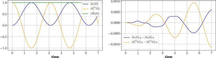
Figure 1: Left panel: Average value of the number operator $\langle\hat{n}_{1}\rangle_{A}$ in blue and of $\langle\hat{\sigma}_{1}^{(z)}\rangle_{A}$ in yellow. The number of excitations $\langle\hat{M}_{1}(t)\rangle_{A}$ is shown in green. Right panel: Difference between the analytic and the numerical calculation, $\langle\hat{n}_{1}\rangle_{A}-\langle\hat{n}_{1}\rangle_{N}$ in blue and $\langle\hat{\sigma}_{1}^{(z)}\rangle_{A}-\langle\hat{\sigma}_{1}^{(z)}\rangle_{N}$ in yellow. Parameters set $\Omega_{1}=.999\omega_{1}$, $\Omega_{2}=.999\omega_{2}$, $\omega_{1}/2\pi=4$GHz, $\omega_{2}/2\pi=5$GHz, $g_{1}=0.04\omega_{1}$, $g_{2}=0.04\omega_{2}$ and $\lambda=10^{-3}\omega_{1}$.

In figure 2 (a) we show the temporal evolution of $\langle\hat{n}_{1}(t)\rangle$ (blue) and $\langle\hat{n}_{2}(t)\rangle$ (green) calculated with the analytic method for Hamiltonian parameters $\Omega_{1}=.999\omega_{1}$, $\Omega_{2}=.999\omega_{2}$, $\omega_{1}/2\pi=4$GHz, $\omega_{2}/2\pi=5$GHz, $g_{1}=0.001\omega_{1}$, $g_{2}=0.001\omega_{2}$ and $\lambda=0.25\omega_{1}$. Here, the atom-field coupling in each cavity is small and there is almost no exchange between the field and the atomic excitations in each cavity. On the other hand, the cavity-cavity coupling is large and there is an important exchange of photons between the cavities. In figure 2 (b) we show the evolution of the total number of excitations in each cavity as well as the total number of excitations in the system calculated with the analytic method. Since the cavity-cavity coupling conserves the total number of photons and the JC Hamiltonians conserve the number of excitations in each cavity, there is an exchange of excitations between the cavities keeping the total number of excitations constant. For this set of Hamiltonian parameters we also made a purely numerical calculation and both calculations yield almost the same results as can be seen in (c) and (d) where we plot the differences between the analytic and the numerical calculations. We can then be sure that the approximations made along the way are justified when either the atom-field coupling is large compared with the cavity-cavity coupling (figure one) and also when the atom-field coupling is small compared with the cavity-cavity coupling (figure 2).

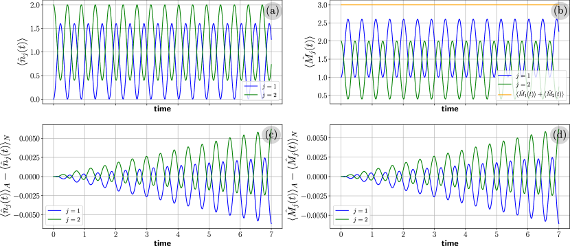
Figure 2: First row: (a) Average value of the number operator $\langle\hat{n}_{1}\rangle_{A}$ in blue and of $\langle\hat{n}_{2}\rangle_{A}$ in green. (b) Average value of the total number of excitations in cavity one $\langle\hat{M}_{1}\rangle_{A}$ in blue, in cavity two $\langle\hat{M}_{2}\rangle_{A}$ in green and in the full system in yellow. Second row: (c) Difference between the analytic and the numerical calculations for the number operator, (d) Difference between the analytic and the numerical calculations for the excitations. Parameters set $\Omega_{1}=.999\omega_{1}$, $\Omega_{2}=.999\omega_{2}$, $\omega_{1}/2\pi=4$GHz, $\omega_{2}/2\pi=5$GHz, $g_{1}=0.001\omega_{1}$, $g_{2}=0.001\omega_{2}$ and $\lambda=.25\omega_{1}$.

Now we consider a case when both coupling parameters are of the same order of magnitude. Take for instance $g_{1}=0.04\omega_{1}$, $g_{2}=0.04\omega_{2}$ and $\lambda=0.08\omega_{1}$. We can see the results in figure 3. In the first row we plot (left panel) $\langle\hat{n}_{1}\rangle$ and $\langle\hat{n}_{2}\rangle$ and (right panel) $\langle\hat{\sigma}_{1}^{(z)}\rangle$, $\langle\hat{\sigma}_{2}^{(z)}\rangle$. Full lines correspond to the analytic calculations and broken lines to the numerical calculation using Python [30]. In the second row we plot the difference between the analytic and the numerical calculations.

The behavior of the average number of photons $\langle\hat{n}_{1}\rangle$ and $\langle\hat{n}_{2}\rangle$ differ significantly with the previous results since in this case the coupling between the cavities is large, as well as the atom-cavity coupling in each one of the cavities. In the right panel we see that the averages $\langle\hat{\sigma}_{1}^{(z)}\rangle$ and $\langle\hat{\sigma}_{2}^{(z)}\rangle$ are oscillating functions of time with a nearly constant amplitude. For both atoms there is a shift in the frequency of the oscillations between the analytic and the numerical calculation. For the atom in cavity one, the frequency (analytic) gets larger while for the atom in cavity two it gets smaller and this means that when $g_{i}\simeq\lambda$ the approximation made in the interaction Hamiltonian $\hat{H}_{I}^{(2)}$ in Eq. 8 is valid for short times. In the second row of the figure we see that the analytic and the numerical results agree quantitatively for short times and there is only a qualitative agreement between both calculations for longer times.

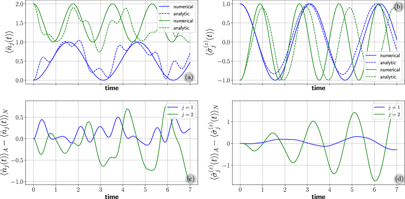
Figure 3: First row:Average value of the number operator $\langle\hat{n}_{1}\rangle$ in blue and of $\langle\hat{n}_{2}\rangle$ in green (left panel). Average value of $\langle\hat{\sigma}_{1}^{(z)}\rangle$ in blue and $\langle\hat{\sigma}_{2}^{(z)}\rangle$ in green (right panel). Second row: Difference between the numerical and the analytic calculations. Cavity one in blue, cavity two in green. Parameters set $\Omega_{1}=.999\omega_{1}$, $\Omega_{2}=.999\omega_{2}$, $\omega_{1}/2\pi=4$GHz, $\omega_{2}/2\pi=5$GHz, $g_{1}=0.04\omega_{1}$, $g_{2}=0.04\omega_{2}$ and $\lambda=0.08\omega_{1}$.

In the following table, we resume the behavior of our analytical method compared with the purely numerical calculation stating the values for the Hamiltonian parameters used.
In all the cases we used: $\omega_{1}/2\pi=4$ GHz, $\omega_{2}/2\pi=5$GHz, $\Omega_{1}=0.999\omega_{1}$, and $\Omega_{2}=0.999\omega_{2}$.

$g_{1}$	$g_{2}$	$\lambda$	Quantit. and Qualit agreement	Qualitative only
$.04\omega_{1}$	$.04\omega_{2}$	$10^{-3}\omega_{1}$	XX
$.001\omega_{1}$	$.001\omega_{2}$	$.25\omega_{1}$	XX
$.01\omega_{1}$	$.01\omega_{2}$	$.02\omega_{1}$	XX
$.4\omega_{1}$	$.4\omega_{2}$	$.001\omega_{1}$	XX
$.04\omega_{1}$	$.04\omega_{2}$	$.08\omega_{1}$		XX

4 Conclusions

In this work we have presented a method to construct an approximate time evolution operator, written in a product form, for a system composed of two coupled cavities containing a two level atom each (two coupled Jaynes Cummings Hamiltonians). The coupling between the cavities conserves the total number of excitations in the system; it creates an excitation in one cavity and kills another one in the other cavity. For uncoupled Jaynes Cummings Hamiltonians the problem is exactly solvable as well as for two coupled cavities with no atoms in them. However, when there are atoms present in the cavities and a coupling between them the problem does not have an exact solution. In order to tackle the problem we first took as unperturbed Hamiltonian the free fields and the two two-level atoms, then we transformed the interaction and obtained a Hamiltonian that could be written as the sum of two independent JC Hamiltonians and a coupling between them. We built the time evolution operator corresponding to the coupling and used it to transform the rest of the interaction. Finally, we approximated this last interaction Hamiltonian as the sum of two independent JC Hamiltonians whose time evolution operators could be written exactly in a product form.

We want to stress the fact that the approximations are made at the level of the interaction Hamiltonian in order to have an approximate Hamiltonian that can be written as a linear combination of operators that form a finite Lie algebra. Then, the corresponding time evolution operator can be obtained exactly by means of the Wei-Norman theorem. Once we have an analytic expression for the time evolution operator, we can propagate any initial state and compute whatever property we are interested on, for example the swapping probability, the Mandel parameter, the Husimi function, the density matrix or the average value of any observable.

In order to test the accuracy of our approximations, we considered a particular initial state and applied to it the full time evolution operator. We evaluated the average number of photons as well as the average value for the atomic state in each cavity and confronted the results with those obtained by a purely numerical calculation solving Scrödinger’s equation for the full Hamiltonian given by Eq. 2. The Hamiltonian parameters for the atom-field coupling and the cavity-cavity coupling were taken from ref. [25] and correspond to actual experimental possibilities. With these Hamiltonian parameters we found a very good agreement with the numerical calculation and a negligible swapping probability. From a comparison with our numerical results we can say that our analytic method can be applied when the atom-field coupling parameters $g_{i}\ll\lambda$ with $\lambda\simeq 10^{-1}\omega_{1}$, also in the oposite limit when the cavity-cavity coupling constant is much smaller than the atom-field coupling ($\lambda\ll g_{i}$ with $g_{i}\simeq 10^{-1}\omega_{1}$) and when both sets of parameters are of the same order of magnitude but with the condition of being much smaller than $\omega_{1}$ (of the order of $10^{-3}\omega_{1}$). When neither of these conditions apply, our method still gives reasonable results at short times and only qualitative agreement for longer times.

Acknowledgement: A. Paredes acknowledges postdoctoral support from DGAPA UNAM, and we thank Reyes García for the maintenance of our computers. We acknowledge partial support from Dirección General de Asuntos del Personal Académico, Universidad Nacional Autónoma de México (DGAPA UNAM) project PAPIIT IN111119.

References

[1] E. T. Jaynes and F. W. Cummings, Proc. IEEE
51, 89 (1963).
[2] B. W. Shore and P. L. Knight, J. of
Mod. Opt.40, 1195 (1993).
[3] Bertet, P., Auffeves, A., Maioli, P.,
Osnaghi, S., Meunier, T., Brune, M., Raimond, J. M., and
Haroche, S. Phys. Rev. Lett. 89, 200402 (2002).
[4] D. Braak, Phys. Rev. Lett. 107, 100401
(2011).
[5] J. Chen, D. Konstantinov and K. Molmer,
Phys. Rev. A 99, 013803 (2019).
[7] B. Sherman and G. Kurizki, Phys. Rev. A
45, R7674 (1992).
[8]K. Vogel, V. M. Akulin, and W.
P. Schleich, Phys. Rev. Lett. 71, 1816 (1993).
[9]H. Moya-Cessa, P. L. Knight, and
A. Rosenhouse-Dantsker, Phys. Rev. A 50, 1814-1821 (1994).
[10]J. R. Kuklinski, J. L. Madajczyk,
Phys. Rev. A 37, 3175-3178 (1988).
[11] R. L. Matos Filho and W. Vogel,
Phys. Rev. Lett. 76, 608 (1996).
[12] R. L. Matos Filho and W. Vogel,
Phys. Rev. A 54, 4560 (1996).
[13] S. Cordero and J. Récamier, J. Phys. A:
Math. Theor. 45, 385303 (2012).
[14] S. Cordero and J. Récamier,
J. Phys. B: At. Mol. Opt. Phys. 44, 135502
(2011).
[15] O. de los Santos-Sánchez, and
J. Récamier, J. Phys. B: At. Mol. Opt. Phys. 45, 015502
(2012).
[16] P. Filipowicz, J. Javanainen, P. Meystre,
Phys. Rev. A 34, 3086 (1996).
[17] H. Moya-Cessa, V. Buzek and P.L. Knight, Opt. Commun. 85, 267-274 (1991).
[18] G. T. Moore, J. Math. Phys. 11, 2679-2691 (1970).
[19] P. D. Nation, J. R. Johansson, M. P. Blencowe and F. Nori, Rev. Mod. Phys. 84, 1-24 (2012).
[20] A. V. Dodonov and V. V. Dodonov, Phys. Rev. A 85, 055805 (2012).
[21] Yan-Ling Li, Mao-Fa Fang, Xing Xiao, Ke Zeng and Chao Wu, J. Phys. B:At. Mol. Phys. 43, 085501 (2010).
[22] H. Mabuchi and A. C. Doherty, Science 298, 1372 (2002).
[23] P. Lähteenmäki, G. S. Paraoanu, J. Hassel and P. J. Hakonen, Proc. Natl. Acad. Sci. USA 110, 4234-4238 (2013).
[24] C. M. Wilson, G. Johansson, A. Pourkabirian, M. Simoen, J. R. Johansson, F. Duty, T. Nori and P. Delsing, Nature 479, 376-379 (2011).
[25] S. Felicetti, M. Sanz, L. Lamata, G. Romero, G.
Johansson, P. Delsing and E. Solano, Phys. Rev. Lett. 113, 093602
(2014).
[26] S. A. Hanoura, M. M. A. Ahmed,
E. M. Khalil, and A. S. F. Obada, Fortschr. Phys. 67, 1800101 (2019).
[27] D. F. V. James and J. Jerke, Can. J. Phys. 85, 625 (2007).
[28]J. Wei and E. Norman, Proc. Am. Math. Soc. 15,
327-334 (1964).
[29] B. M. Rodríguez-Lara, H. M. Moya-Cessa, J. Phys. A: Math. Theor. 46, 095301 (2013).
[30] J. R. Johansson, P. D. Nation, and F. Nori,
”QuTiP2: A Python framework for the dynamics of open quantum
systems”, Comp. Phys. Comm. 184, 1234 (2013).