3D Distribution Map of Hi Gas and Galaxies around an Enormous Ly$\alpha$ Nebula and Three QSOs at $z=2.3$
Revealed by the Hi Tomographic Mapping Technique

Abstract

We present an IGM Hi tomographic map in a survey volume of $16\times 19\times 131\ h^{-3}{\rm comoving\ Mpc}^{3}$ (cMpc³) centered at MAMMOTH-1 nebula and three neighboring quasars at $z=2.3$. MAMMOTH-1 nebula is an enormous Ly$\alpha$ nebula (ELAN), hosted by a type-II quasar dubbed MAMMOTH1-QSO, that extends over $1\ h^{-1}$ cMpc with not fully clear physical origin. Here we investigate the Hi-gas distribution around MAMMOTH1-QSO with the ELAN and three neighboring type-I quasars, making the IGM Hi tomographic map with a spatial resolution of $2.6\ h^{-1}$ cMpc. Our Hi tomographic map is reconstructed with Hi Ly$\alpha$ forest absorption of bright background objects at $z=2.4-2.9$: one eBOSS quasar and 16 Keck/LRIS galaxy spectra. We estimate the radial profile of Hi overdensity for MAMMOTH1-QSO, and find that MAMMOTH1-QSO resides in a volume with fairly weak Hi absorption. This suggests that MAMMOTH1-QSO may have a proximity zone where quasar illuminates and photo-ionizes the surrounding Hi gas and suppresses Hi absorption, and that the ELAN is probably a photo-ionized cloud embedded in the cosmic web. The Hi radial profile of MAMMOTH1-QSO is very similar to those of three neighboring type-I quasars at $z=2.3$, which is compatible with the AGN unification model. We compare the distributions of the Hi absorption and star-forming galaxies in our survey volume, and identify a spatial offset between density peaks of star-forming galaxies and Hi gas. This segregation may suggest anisotropic UV background radiation created by star-forming galaxy density fluctuations.

1 Introduction

Enormous Ly$\alpha$ Nebulae (ELANe) are extremely extended Ly$\alpha$ nebulae discovered around $z\sim 2$ radio-quiet quasars (e.g., Cantalupo et al., 2014; Kikuta et al., 2019; Cai et al., 2019). Since their Ly$\alpha$ emission extends to $>1\ h^{-1}$ comoving Mpc (cMpc) beyond the virial diameters of their host quasars, the major origin of ELANe is predicted to be quasar photo-ionization of neutral hydrogen (Hi) gas embedded in the cosmic web (e.g., Cantalupo et al., 2012). However, the gas distribution around ELANe has been poorly investigated in previous studies.

Recently, one of the largest ELANe, MAMMOTH-1, has been identified at $z=2.32$ by Cai et al. (2017a). MAMMOTH-1 hosts a type-II quasar (hereafter MAMMOTH1-QSO) and, interestingly, resides in a Ly$\alpha$ emitter (LAE) overdense region that has been originally discovered with a strong Hi absorber group, dubbed BOSS1441, with multiple background quasar spectra in the Mapping the Most Massive Overdensities through Hydrogen (MAMMOTH) survey (Cai et al., 2017b). Although Cai et al. (2017b) have revealed the existence of the significant Hi overdensity around MAMMOTH-1 on a large scale of $\sim 20\ h^{-1}$ cMpc, it is yet unknown whether MAMMOTH1-QSO photo-ionizes the surrounding Hi gas or not on smaller scales.

To investigate the Hi gas distribution on such small scales, one can use galaxies instead of quasars as background sources thanks to their higher number densities (e.g., Mawatari et al., 2017; Hayashino et al., 2019). For this purpose, a powerful technique called Hi tomography has been established by Lee et al. (2014a, b). This technique allows us to reconstruct three-dimensional (3D) Hi large-scale structures (LSSs) based on Hi Ly$\alpha$ forest absorption lines detected in background source spectra (See also, Lee et al. 2016, 2018).

In this study, we map out the Hi gas distribution around MAMMOTH1-QSO with the Hi tomography technique based on Ly$\alpha$ forest absorption probed with background quasar and galaxy spectra. In addition, by combining results of Ly$\alpha$ forest absorption analyses for background quasars whose projected distances from MAMMOTH1-QSO are relatively large, up to $\sim 200h^{-1}$ cMpc, we estimate the Hi radial profile of MAMMOTH1-QSO over a wide range of scales and make comparisons with quasars at similar redshifts as well as the LAE overdensity distribution.

This paper is organized as follows. In Section 2, we introduce our background source sample and describe their spectroscopic data. In Section 3, our spectral analyses and Hi tomographic reconstruction are described. We present results and discussions in Section 4. Finally, we summarize our findings in Section 5. Throughout this paper, we use a cosmological parameter set $(\Omega_{m},\Omega_{\Lambda},\Omega_{b},h)$=$(0.26,0.74,0.045,0.70)$ consistent with the nine-year WMAP result (Hinshaw et al., 2013). We refer to kpc and Mpc in physical (comoving) units as pkpc and pMpc (ckpc and cMpc), respectively. All magnitudes are in AB magnitudes (Oke & Gunn, 1983).

2 Data and Sample

To study the Hi gas distribution around MAMMOTH1-QSO over a wide range of scales, we need spectra of background quasars and galaxies. In this section, we construct a spectroscopic sample of background quasars and galaxies around the sky position of MAMMOTH1-QSO. The basic properties of MAMMOTH1-QSO are summarized in Table 1.

Table 1: Properties of MAMMOTH1-QSO

Source	R.A.	Decl.	$z_{\rm spec}$	$V$	Ref.
	(J2000)	(J2000)		(mag)
MAMMOTH1-QSO	14 41 24.46	+40 03 09.20	$2.319$	$24.20$	C17

2.1 Background Quasars

We select background quasars around MAMMOTH1-QSO from the SDSS DR14 quasar catalog (hereafter DR14Q; Pâris et al., 2018), which includes all quasars identified by the SDSS-IV/eBOSS survey (Myers et al., 2015). The eBOSS spectra have a spectral resolution of $R\equiv\lambda/\Delta\lambda\approx 2000$ covering a wavelength range of $3600$–$10400$Å, which is sufficient for our purpose.

First, we search for quasars in a $6\fdg 0\times 6\fdg 0$ field around MAMMOTH1-QSO (the $6\fdg 0$ scale corresponds to a span of 400 $h^{-1}$ cMpc). We then select quasars whose emission redshifts are in the range of $z=2.4$–$2.9$ so that we can probe Ly$\alpha$ forest absorption lines at the redshift of MAMMOTH1-QSO in the background quasars’ rest-frame $1041$–$1185$Å spectral region to avoid contamination of Hi Ly$\beta$ absorption and stellar/interstellar absorption lines associated with the quasar host galaxies (e.g., Mukae et al., 2017). These two criteria yield $240$ DR14Q quasars.

To obtain robust measurements of Ly$\alpha$ forest absorption, we check the qualities of the eBOSS spectra and remove quasars whose spectra do not meet additional criteria described below. We require the eBOSS spectra have a median signal-to-noise ratio (S/N) $\geq 2$ over their Ly$\alpha$ forest wavelength range (i.e., $1041$–$1185$Å in the rest-frame). In addition, we remove quasars whose spectra have broad absorption lines by applying BI $<200$ km s^-1 in the DR14Q catalog, where BI (BALnicity Index) is a measure of the strength of an absorption trough calculated for the Civ emission line. We also remove quasars whose spectra show damped Ly$\alpha$ systems (DLAs) in the Ly$\alpha$ forest wavelength range, based on the DLA catalog of Noterdaeme et al. (2012) and their updated one for the SDSS DR12 quasars (Pâris et al., 2017). For quasars that have no SDSS DR12 counterpart, we visually inspect the eBOSS spectra and remove them if they show signatures of DLAs in their Ly$\alpha$ forest wavelength range. Our careful selection results in a sample of $117$ background quasars for our subsequent analyses.

For convenience, we divide the $6\fdg 0\times 6\fdg 0$ field around MAMMOTH1-QSO into three regions, BQ1, BQ2, and BQ3 as illustrated in Figure 1. The boundary between BQ1 and BQ2 is defined with a rectangle whose corners are ($\Delta$R.A., $\Delta$Decl.) = ($-0\fdg 19$, $-0\fdg 21$), ($-0\fdg 19$, $+0\fdg 058$), ($+0\fdg 11$, $+0\fdg 058$), and ($+0\fdg 11$, $-0\fdg 21$) relative to the coordinate of MAMMOTH1-QSO, so that the 16 $h^{-1}$ cMpc $\times$ 19 $h^{-1}$ cMpc area of the BQ1 region can cover the position of MAMMOTH1-QSO as well as the LAE overdense region for comparison in Section 4.3. The boundary between BQ2 and BQ3 is defined with a rectangle whose corners are $\Delta$R.A. = $\pm 0\fdg 4$ and $\Delta$Decl. = $\pm 0\fdg 3$. This corresponds to a 40 $h^{-1}$ cMpc $\times$ 41 $h^{-1}$ cMpc rectangle atop the entire BOSS1441 field (Cai et al., 2017b). In the BQ1, BQ2, and BQ3 regions, the numbers of our background quasars are 1, 4, and 112, respectively. The distributions of the background quasars in BQ1 and BQ2 regions are presented in Figure 1. The basic properties of the background quasars in the BQ1 and BQ2 regions are provided in Tables 2 and 3, respectively.

Note that Cai et al. (2017b) have identified the strong Hi absorber group based on the spectra of these five background quasars as well as an additional one in the BQ1–2 regions. In our analyses we do not use the spectrum of the additional quasar, since its redshift is $z>2.9$ and there is a possibility that the spectrum is contaminated by the Ly$\beta$ absorption and/or stellar/interstellar absorption due to the quasar host galaxy.

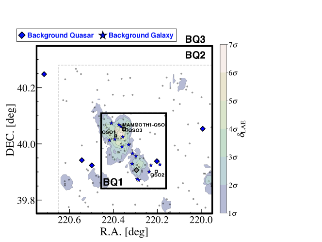
Figure 1: Sky distribution of our background quasars and galaxies in the BQ1 and BQ2 regions. The blue diamonds (stars) represent the positions of our background quasars (galaxies) at $z=2.4$–$2.9$. The gray diamond indicates a $z>2.9$ quasar that is used in Cai et al. (2017b) in addition to the other five quasars, although we do not use it in our analyses (for details, see Section 2.1). The double square is the position of MAMMOTH1-QSO at $z=2.32$ and the single squares are those of three neighboring quasars at $z\simeq 2.3$, QSOs 1–3 (Section 4.2.2). The dark-gray dots are $z\simeq 2.32$ LAEs found in the previous work (Cai et al. 2017b), whose survey area is shown with light-gray dashed lines. The color contours represent LAE overdensities $\delta_{\rm LAE}$ calculated in Section 4.3.

Table 2: Background objects for Hi tomographic reconstruction in the BQ1 region

Source	R.A.	Decl.	$z_{\rm spec}$	$g$	$V$	Exposure Time	Sample
	(J2000)	(J2000)		(AB)	(AB)	(s)
BQ1-5172-56071-0534	14 40 48.56	+39 56 18.39	2.543	20.04	-	-	eBOSS
20170827_M1_05	14 41 19.44	+39 59 49.52	2.509	-	24.04	9000	LRISs
20170827_M1_07	14 41 26.77	+39 59 25.01	2.816	-	23.40	9000	LRISs
20170827_M1_22	14 41 27.98	+40 03 43.31	2.510	-	24.50	9000	LRISs
20170827_M1_24	14 41 30.05	+40 04 05.59	2.671	-	23.58	9000	LRISs
20160510_M2_05	14 41 11.50	+39 57 24.08	2.546	-	24.11	5400	LRISa
20160510_M2_10	14 41 16.63	+39 58 51.56	2.598	-	23.21	5400	LRISa
20160510_M2_25	14 41 34.49	+40 00 58.68	2.795	-	23.61	5400	LRISa
20160509_M1_11	14 41 40.29	+40 00 46.08	2.557	-	23.05	4000	LRISa
20160509_M1_23	14 41 38.31	+40 04 23.49	2.786	-	22.84	4000	LRISa
20160405_M1_05	14 41 25.85	+40 01 31.40	2.795	-	22.82	6000	LRISa
20160405_M2_08	14 41 10.15	+39 52 28.88	2.791	-	24.27	6000	LRISa
20160405_M2_10	14 41 15.62	+39 55 43.97	2.512	-	24.42	6000	LRISa
20160405_M2_11	14 41 08.38	+39 52 15.59	2.497	-	23.68	6000	LRISa
20160405_M2_20	14 40 56.98	+39 54 03.24	2.703	-	24.34	6000	LRISa
20160405_M2_27	14 40 55.13	+39 55 25.70	2.840	-	24.37	6000	LRISa
20160405_M2_35	14 40 45.31	+39 55 35.76	2.598	-	23.07	6000	LRISa

Table 3: Background quasars in the BQ2 region

Source	R.A.	Decl.	$z_{\rm spec}$	$g$	Ref.
	(J2000)	(J2000)		(AB)
BQ2-5171-56038-0020	14 39 58.45	+40 03 13.99	2.422	20.20	DR14Q
BQ2-8498-57105-0478	14 41 59.76	+39 55 25.32	2.546	19.47	DR14Q
BQ2-5172-56071-0616	14 42 10.56	+39 56 31.92	2.612	20.99	DR14Q
BQ2-5172-56071-0608	14 42 51.84	+40 14 53.52	2.547	20.86	DR14Q

2.2 Background Galaxies

2.2.1 Candidate Selection

As shown in Figure 1, the number of our background quasars near MAMMOTH1-QSO is small, only one in the BQ1 region. To investigate the Hi gas distribution around MAMMOTH1-QSO down to a small scale, we need a sample of close background galaxies at $z=2.4$–$2.9$ near MAMMOTH1-QSO.

For this purpose, we produce a multiwavelength catalog across the BQ1 region based on optical ($U$, $V$, and $i$) and near-IR ($J$ and $H$) imaging data obtained by Cai et al. (2017b) and Z. Cai et al. (in prep.) with the Large Binocular Camera (LBC; Pedichini et al., 2003) on the Large Binocular Telescope (LBT) and the Wide Field Camera (WFCAM; Casali et al., 2007) on the United Kingdom Infrared Telescope (UKIRT), respectively. We match the point spread functions (PSFs) of these images to that of the $H$-band image whose FWHM ($0\farcs 9$) is the largest among them. The $5\sigma$ limiting magnitudes in the $U$, $V$, $i$, $J$, and $H$ bands measured with $2\farcs 0$ diameter apertures are $26.6$, $26.2$, $26.1$, $23.7$, and $23.1$ mag, respectively. We then create a multiwavelength source catalog by running SExtractor (Bertin & Arnouts, 1996) in dual image mode. Colors of the detected sources are measures with $2\farcs 0$ diameter apertures.

Based on the multiwavelength catalog, we estimate photometric redshifts of the detected sources to select background galaxy candidates at $z=2.4$–$2.9$. First of all, we apply a magnitude cut of $V<24.85$ mag so that we can select background galaxy candidates whose continuum emission can be detected with sufficiently high S/Ns in subsequent spectroscopic observations. We then estimate their photometric redshifts with the EAZY software (Brammer et al., 2008) by fitting spectral energy distribution (SED) templates to the observed photometric data points. The SED templates are produced with the stellar population synthesis model of Bruzual & Charlot (2003). We adopt the Chabrier initial mass function (Chabrier, 2003), a constant star formation for $0.1$ Gyr, and a fixed metallicity of $Z=0.2Z_{\odot}$. The metallicity is chosen to be close to the metallicity estimates of star-forming galaxies in Pettini et al. (2000) and Pettini et al. (2001). We apply the Calzetti dust attenuation (Calzetti et al., 2000) with $E(B-V)=$ 0.0, 0.15, 0.30, and 0.45. We also apply attenuation by IGM absorption with a model of Inoue et al. (2014). We require background galaxy candidates to have a photometric redshift whose $1\sigma$ confidence interval is within the redshift range of $z=2.4$–$2.9$. The $1\sigma$ errors on the photometric redshift from the used software are $\sim 0.17$. This selection yields a sample of $131$ background galaxy candidates in BQ1.

2.2.2 Follow-up Spectroscopy

We carried out spectroscopic observations for our background galaxy candidates using the Low Resolution Imaging Spectrometer (LRIS) Double-Spectrograph (Oke et al., 1995) on the Keck I telescope on 2017 August 27 (UT) (PI: S. Mukae). We used the d560 dichroic with the B600/4000 grism on the blue arm, resulting in a wavelength coverage of 3800–5500Å. The observations were made in the multi-object slit (MOS) mode. We designed one mask targeting background galaxy candidates around MAMMOTH1-QSO with $1\farcs 0$ slit width, yielding a spectroscopic resolution of $R\equiv\lambda/\Delta\lambda\approx 1000$. We select 25 background galaxies from our 131 background galaxy candidates based on photometric redshift probability, source brightness, and uniformity on the sky. The total exposure time was 9000 s. The sky conditions were clear throughout the observing run, with an average seeing size of $0\farcs 95$.

We reduce the LRIS data with the Low-Redux package in the public XIDL pipeline. The pipeline conducts bias subtraction, flat fielding with dome flat and twilight flat data, wavelength calibration with arc data, cosmic ray rejection, source identification, spectral trace determination, sky background subtraction, and distortion correction. We then extract one-dimensional (1D) spectra of the identified sources from the reduced two-dimensional (2D) spectra and combine them to obtain their stacked 1D spectra.

2.2.3 Archival Search

In addition to our own observations, two other LRIS programs were conducted for the BOSS1441 field in the MOS mode on 2016 April 5 (UT) (PI: X. Fan) and 2016 May 9–10 (UT) (PI: X. Prochaska) by using the same dichroic and grism as ours. Although the original aim of their LRIS programs is to identify associated galaxies in the BOSS1441 overdense region at $z=2.32$ (Z. Cai et al., private communication), there is a possibility that some background galaxies at $z=2.4-2.9$ are included as targets in the MOS masks and spectroscopically identified by chance. Thus, we download raw LRIS data obtained in the two programs from the Keck Observatory Archive (KOA) and reduce them in the same manner as for our LRIS data.

2.2.4 Sample Construction for Our Analyses

We determine spectroscopic redshifts ($z_{\rm spec}$) of the observed sources based on the LRIS spectra obtained in Sections 2.2.2 and 2.2.3. We fit the galaxy spectrum template of Shapley et al. (2003) to the LRIS spectra and determine the best-fit $z_{\rm spec}$ by the minimum value of $\chi^{2}$. We find that $20$ galaxies have $z_{\rm spec}$ values in the range of $2.4$–$2.9$.

To obtain robust measurements of Ly$\alpha$ forest absorption, in the same way as for the background quasars, we further require that the spectra of background galaxies have a median S/N $\geq 2$ in the Ly$\alpha$ forest wavelength range of $1041$–$1185$Å in the rest-frame. In addition, based on our visual inspection, we remove a galaxy whose spectrum shows a possible feature of a DLA in the Ly$\alpha$ forest wavelength range. These selections result in a sample of $16$ background galaxies. The basic properties of the $16$ background galaxies in the BQ1 region are summarized in Table 2.

Figure 2 shows the positions of the background quasar and galaxies in the BQ1 region. The mean (median) transverse sightline separation is ${\langle d}_{\perp}\rangle\simeq 2.6\ (2.7)\ h^{-1}$ cMpc, which is comparable to that of the Hi tomographic map of Lee et al. (2014b). The filling factor of the sky coverage, which is defined as the fraction of the regions around the sightlines of the background sources within ${\langle d}_{\perp}\rangle$ in the BQ1 region, is about $0.45$.

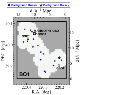
Figure 2: Sky distribution of our background sources in the BQ1 region. The blue diamond and stars represent the positions of our background quasar and galaxies, respectively. The white area highlights regions around the sightlines around the background sources within the mean transverse sightline separation ${\langle d}_{\perp}\rangle=2.6h^{-1}$ cMpc. The double square denotes the position of MAMMOTH1-QSO and the single squares show the those of three neighboring quasars, QSOs 1–3 (Section 4.2.2). The top and right axes are co-moving separations relative to the bottom right corner coordinate of the BQ1 region, (R.A., Decl.) = ($220\fdg 16$, $39\fdg 84$).

3 Analysis

3.1 Ly$\alpha$ Forest Transmission

To measure the strengths of Ly$\alpha$ forest absorption around MAMMOTH1-QSO along the lines of sight to the background quasars and galaxies, we estimate the Ly$\alpha$ forest transmission,

$$F(z)=f_{\rm obs}/f_{\rm int},$$ (1)

where $z$ is the Ly$\alpha$ absorber redshift derived from the observed wavelength $\lambda_{\rm obs}$ (i.e., $\lambda_{\rm obs}/1216$Å-1), $f_{\rm obs}$ is the observed continuum flux density, and $f_{\rm int}$ is the intrinsic continuum flux density that is not affected by the Ly$\alpha$ forest absorption due to the IGM. The transmission $F(z)$ is computed pixel by pixel with a pixel scale of 0.8 (1.2) Å for our eBOSS (LRIS) spectra.

We estimate $f_{\rm int}$ based on the spectra of the background quasars and galaxies in the BQ1–3 regions by applying the mean flux regulated principal component analysis (MF-PCA) continuum fitting technique (Lee et al., 2012) with the code developed by Lee et al. (2013) (see also Lee et al. 2014b). This technique is composed of two steps. The first step is to fit spectral templates of quasars and galaxies with the observed spectra in the redward of Ly$\alpha$ to obtain initial guesses of their continuum spectra in the blueward of Ly$\alpha$. We use the spectral templates of quasars and galaxies constructed by Suzuki et al. (2005) and Berry et al. (2012), respectively. The second step is to further adjust the continuum spectra by multiplying and fitting a linear function, ($a_{\rm MF}$ + $b_{\rm MF}$ $\lambda_{\rm rest}$), where $a_{\rm MF}$ and $b_{\rm MF}$ are free parameters for the fit, and $\lambda_{\rm rest}$ is the rest-frame wavelength. This fit is performed for the continuum spectra within the Ly$\alpha$ forest wavelength range of 1041-1185 Å in the rest-frame to yield a mean transmission (using Equation (1)) consistent with previous measurements of the cosmic mean Ly$\alpha$ forest transmission, ${F_{\rm cos}(z)}$. We adopt ${F_{\rm cos}(z)}$ estimated by Faucher-Giguère et al. (2008),

$${F_{\rm cos}(z)}=\exp[-0.00185(1+z)^{3.92}],$$ (2)

where $z$ is the Ly$\alpha$ absorber redshift. Both the examples of continuum estimates for our background quasar and galaxy spectra are shown in Figure 3. Although the MF-PCA technique introduces a discontinuity at 1185 Å in the final continuum, the discontinuity does not affect our analysis in the Ly$\alpha$ forest wavelength range blueward of 1185 Å (see Lee et al. 2013, 2012 for more details).

There is a possibility that the strong Hi absorption group at $z=2.32\pm 0.03$ found by Cai et al. (2017b) could bias the intrinsic continuum estimate. To avoid possible contamination of their strong Ly$\alpha$ absorption, we mask out the wavelength range of $4036\pm 36$Å in the MF-PCA fitting.

We then obtain $F(z)$ by using Equation (1). Since the strong stellar and interstellar absorption lines of Nii $\lambda 1084$ and Ciii $\lambda 1175$ associated with background sources in the Ly$\alpha$ forest wavelength range could bias the results, we do not use the spectra in the wavelength ranges of $\pm 5$Å around these lines for conservative estimates in the following analyses. The uncertainties of $F(z)$ are calculated from the uncertainties of the $f_{\rm obs}$ measurements and the $f_{\rm int}$ estimates based on the MF-PCA continuum fitting, the latter of which are evaluated by Lee et al. (2012) as a function of redshift and median S/N over the Ly$\alpha$ forest wavelength range (see their Figure 8). Specifically, we adopt MF-PCA continuum fitting errors of $7$%, $6$%, and $4$% for spectra with median S/Ns over the Ly$\alpha$ forest wavelength range of $2$–$4$, $4$–$10$, and $>10$, respectively.

Based on the estimated $F(z)$ and the cosmic mean Ly$\alpha$ forest transmission $F_{\rm cos}(z)$, we calculate the Hi overdensity $\delta_{F}$, following the definition introduced by Lee et al. (2014a, b),

$$\delta_{F}=\frac{F(z)}{F_{\rm cos}(z)}-1,$$ (3)

where negative values correspond to strong Hi Ly$\alpha$ absorption. The uncertainties of $\delta_{F}$ are calculated based on the uncertainties of $F(z)$. We confirm that a systematic effect of using different prescriptions of $F_{\rm cos}(z)$ obtained by Becker et al. (2013) and Inoue et al. (2014) is minor, only within $2$%, which is not as large as the uncertainties of $F(z)$.

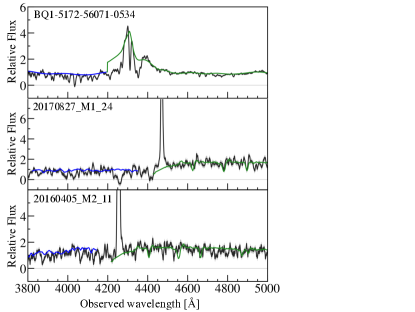
Figure 3: Example spectra of our background sources in the BQ1 region. Top panel is an eBOSS spectrum of a background quasar. Middle and bottom panels are Keck/LRIS spectra of background galaxies. The black lines depict the spectra smoothed with $1.25$ $h^{-1}$ cMpc scales along the sightlines and the grey shades represent the uncertainties. The grey lines are the flux zero level. The green curve(s) in the top (middle and bottom) panel(s) are the Suzuki et al. (2005) (Shapley et al. 2003) template overplotted at the source redshifts. The blue curve(s) in the top (middle and bottom) panel(s) are the Suzuki et al. (2005) (Berry et al. 2012) template representing the estimated continuum (continua) within the Ly$\alpha$ forest wavelength range (for details, see Section 3.1).

3.2 Hi Tomographic Reconstruction

For the BQ1 region, where the background sightline density is high, we carry out an Hi tomographic reconstruction to reveal the 3D distribution of Hi gas near MAMMOTH1-QSO with the code developed by Stark et al. (2015). The reconstruction code performs the Wiener filtering for the estimated $\delta_{F}$ values along the sightlines of our background quasar and galaxies. The Wiener filtering is based on a gaussian smoothing with the scale of $\langle d_{\perp}\rangle$, which determines the spatial resolution of our tomographic map. We adopt a grid size of $0.5\ h^{-1}$ cMpc, which is sufficiently small compared to ${\langle d}_{\perp}\rangle$. We choose a redshift range of $z=2.25$–$2.40$ that covers a large distance of $\sim\pm 65\ h^{-1}$ cMpc from MAMMOTH1-QSO at $z=2.32$ in the redshift direction, giving an overall volume of $16\ \times 19\ \times 131\ h^{-3}{\rm cMpc}^{3}$. More details about the reconstruction process is presented in Stark et al. (2015) and Lee et al. (2018).

There is is a possibility that sightlines used in the Hi tomography could undersample small Hi gas clumps in the Ly$\alpha$ forest on scales below ${\langle d}_{\perp}\rangle$. We thus do not use the small-scale gas distributions in our discussions from Section 4.1. The simulation studies of Lee et al. (2014a) demonstrated that an Hi tomography pixel could have the $\delta_{F}$ error of $\leq 0.05$ due to the sightline undersampling of the Ly$\alpha$ forest.

Note that we do not reconstruct Hi tomographic maps for the BQ2-3 regions due to the coarse sightline distributions whose sightline separations are $\sim$15-20 $h^{-1}$ cMpc. Instead, we use the BQ2-3 background quasars for large-scale $\delta_{F}$ measurements along the sightlines (Section 4.2).

4 Results and Discussion

4.1 Hi Tomographic Map

Figure 4 presents the resulting Hi tomographic map for the BQ1 region. Our tomographic map shows $\delta_{F}$ values in the range of $-0.6<\delta_{F}<0.4$, revealing the existence of Hi overdense ($\delta_{F}\simeq-0.3-(-0.2)$) and underdense ($\delta_{F}\simeq 0.3-0.2$) LSSs with sizes of $10$–$20\ h^{-1}{\rm cMpc}$ around MAMMOTH1-QSO for the first time. In this region, the strong Hi absorption group at $z=2.32$ has been found in the previous work based on only the six background quasar spectra (Cai et al., 2017b) as mentioned in Section 2.1. Thanks to the higher sightline density of our background source sample in this field, our results unveil the inhomogeneous distribution of Hi gas around MAMMOTH1-QSO.

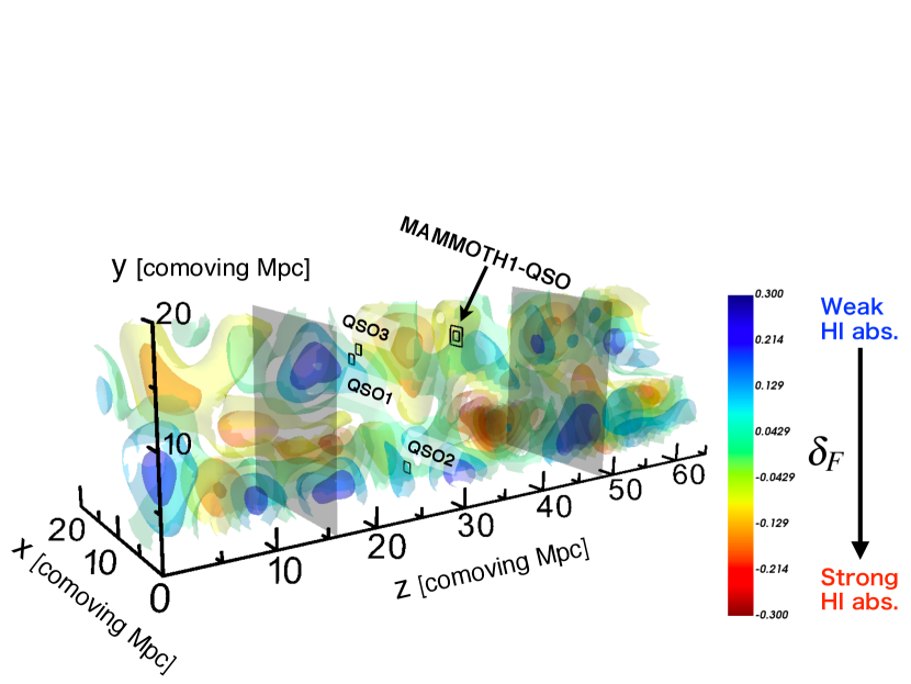
Figure 4: Hi tomographic map reconstructed based on Ly$\alpha$ forest absorption along the sightlines of our background quasar and galaxies in the BQ1 region. Here we present a zoomed map at $z=2.28$–$2.35$ to clearly show the Hi overdensity distribution around MAMMOTH1-QSO, although we obtain the Hi tomographic map in the redshift range of $z=2.25$–$2.40$. The spatial axes of R.A., Decl., and $z$ are represented as $x$, $y$, and $z$ in co-moving scales, respectively. The color contours show the Hi overdensity $\delta_{F}$, whose maximum (minimum) scale is set to $+0.3$ ($-0.3$) for visualization, although some regions show higher or lower $\delta_{F}$ values in the range of $-0.6<\delta_{F}<0.4$. The double square indicates the position of MAMMOTH1-QSO. The single squares show the three neighboring quasars, QSOs 1–3 (Section 4.2.2). Note that the redshift range between the two gray planes at $z\simeq 2.30$ and $z\simeq 2.33$ correspond to the FWHM of the narrowband filter NB403, which is used in Cai et al. (2017a, b) to detect LAEs at $z\simeq 2.30$–$2.33$ in the BOSS1441 field (Section 4.3).

4.2 Hi Radial Profile

4.2.1 Hi gas around MAMMOTH1-QSO

In the BOSS1441 region, there is a type-II quasar dubbed MAMMOTH1-QSO that has one of the largest ELANe, MAMMOTH-1 nebula at $z=2.32$ (Cai et al., 2017a). Since the Ly$\alpha$ emission spatially extends to $>1\ h^{-1}$ cMpc beyond virial diameter of the host quasar, the origin of MAMMOTH-1 nebula is thought to be quasar photo-ionization of Hi gas cloud embedded in the cosmic web (e.g., Cantalupo et al., 2012). Thus, the Hi absorption around the MAMMOTH1-QSO is expected to be suppressed.

We derive the radial profile of Hi overdensity $\delta_{F}$ around MAMMOTH1-QSO (hereafter Hi radial profile). Within the BQ1 region, we use the Hi tomographic map to calculate spherically averaged $\delta_{F}$ as a function of the 3D distance from MAMMOTH1-QSO, which is defined as

$$R_{\rm 3D}\equiv\sqrt{d_{\rm RA}^{2}+d_{\rm Dec}^{2}+d_{z}^{2}}.$$ (4)

$d_{\rm RA}$, $d_{\rm Dec}$, and $d_{z}$ are the co-moving distances from MAMMOTH1-QSO under the assumption that the Hi absorbers have zero peculiar velocities relative to MAMMOTH1-QSO.

To estimate the uncertainties of the spherically averaged $\delta_{F}$ values, we create mock Ly$\alpha$ forest transmission data by adding noise to the obtained $F(z)$ data based on the uncertainties of $F(z)$ estimated in Section 3.1, and calculate the $\delta_{F}$ values for the mock data along the $17$ sightlines. We then obtain a mock Hi tomographic map, and compute spherically averaged $\delta_{F}$ values as a function of $R_{\rm 3D}$. We repeat this process 1000 times and obtain $68$% intervals as the $1\sigma$ confidence intervals. Note that the typical $1\sigma$ uncertainty of $\delta_{F}$ for a pixel in the Hi tomographic map is found to be about $0.08$.

The Hi tomographic map allows us to obtain the Hi radial profile up to around $R_{\rm 3D}=6$ pMpc, which is limited due to the size of our Hi tomographic map. To extend our measurements beyond $6$ pMpc, obtain spherically averaged $\delta_{F}$ values based on the $\delta_{F}$ measurements along the sightlines of the background quasars in the BQ2–3 regions. Thanks to the large field coverage, our Hi radial profile measurements probe up to about $100$ pMpc around MAMMOTH1-QSO.

Figure 5 shows the obtained Hi radial profile around MAMMOTH1-QSO. We find that $\delta_{F}$ decreases (i.e., the strength of Hi absorption increases) with increasing $R_{\rm 3D}$ up to $\simeq 3$ pMpc from $\delta_{F}\simeq 0$ to $\delta_{F}=-0.06\pm 0.02$, and $\delta_{F}$ slightly increases at larger distances. In other words, the Hi radial profile of MAMMOTH1-QSO shows a possible turnover at $R_{\rm 3D}\simeq 3$ pMpc, indicating that MAMMOTH1-QSO resides in a volume with fairly weak Hi absorption. This tendency at small distances is opposite to that found for moderately bright galaxies at similar redshifts (e.g., Rudie et al. 2012; Rakic et al. 2012; Turner et al. 2014); the Hi gas absorption around galaxies is stronger at smaller galactocentric radii. Our results may suggest that MAMMOTH1-QSO has a proximity zone where Hi gas is photo-ionized and Hi absorption is suppressed due to strong ionizing radiation from MAMMOTH1-QSO. In this picture, the ELAN around MAMMOTH1-QSO may be a photo-ionized cloud embedded in the cosmic web.

We caution readers that our suggested picture is based on the tomographic map data as well as the background sources, which are partially sampling the space around MAMMOTH1-QSO (see Figures 1 and 2). Although, we find a possible turnover in the Hi radial profile, the validity of this picture should be statistically tested with more background sources in future work.

Note that the Hi radial profile shows negative $\delta_{F}$ values at $R_{\rm 3D}\simeq 10$–$30$ pMpc, which is consistent with the detection of the strong Hi absorption group found by Cai et al. (2017b). We also confirm that the $\delta_{F}$ values reach the cosmic average ($\delta_{F}=0$) at a large scale of $R_{\rm 3D}\simeq 100$ pMpc.

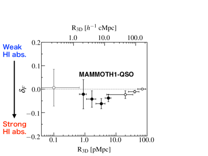
Figure 5: Hi radial profile around MAMMOTH1-QSO as a function of 3D distance $R_{\rm 3D}$ from it. The black filled (open) circles show our results obtained in the BQ1 region (BQ2 and BQ3 regions). The black horizontal bars represent the measurement boundaries for the average. The horizontal dotted line represents the cosmic average of the Hi absorption at $z=2.32$. The gray open circle presents the measurement of Hi tomography map pixel where MAMMOTH1-QSO resides and whose spatial scale is below the spatial resolution which is shown as gray horizontal bars for reference.

4.2.2 Comparisons with Type-I Quasars

Since MAMMOTH1-QSO is categorized as a type-II quasar (Cai et al., 2017a), it is interesting to compare its Hi radial profile with those of type-I quasars.

To make comparisons with type-I quasars, we select three type-I quasars (QSO1, QSO2, and QSO3) within our Hi tomographic map from the DR14Q catalog and calculate spherically averaged Hi radial profiles around them in the same manner as that for MAMMOTH1-QSO. The basic properties of QSOs 1–3 are summarized in Table 4 and their positions in the tomographic map are shown in Figure 4.

Figure 6 compares the Hi radial profiles of QSOs 1–3 with that of MAMMOTH1-QSO. We find that their Hi radial profiles are similar to that of MAMMOTH1-QSO across $100$ pMpc, showing a common turnover at $R_{\rm 3D}\simeq 3$ pMpc. We should be cautious of the partial sampling around QSOs 1–3 (see Section 4.2.1) This result may indicate that spherically averaged Hi gas distributions around type-I and type-II quasars are similar, which is compatible with the AGN unification model (e.g., Antonucci, 1993; Elvis, 2000): type-I quasars can ionize gas preferentially in the line-of-sight direction, while type-II quasars can ionize gas in the transverse directions rather than the line-of-sight direction.

Table 4: Three neighboring quasars in the Hi tomographic map selected from the DR14Q catalog

Source	R.A.	Decl.	$z_{\rm spec}$	$g$	Ref.
	(J2000)	(J2000)		(AB)
QSO1	14 41 33.75	+40 01 42.78	$2.306$	20.66	DR14Q
QSO2	14 40 49.14	+39 54 07.51	$2.306$	21.02	DR14Q
QSO3	14 41 21.66	+40 02 58.82	$2.305$	21.87	DR14Q

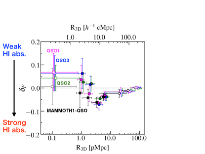
Figure 6: Same as Figure 5, but for the three neighboring quasars (QSOs 1–3) as well as MAMMOTH1-QSO. The black, magenta, green, and blue circles represent MAMMOTH1-QSO, QSO1, QSO2, and QSO3, respectively. The colored circles are slightly offset for clarity. The innermost open circles present the measurements of Hi tomography map pixels where QSOs 1–3 and MAMMOTH1-QSO reside and whose spatial scales are below the spatial resolution which is shown as the attached horizontal bars for reference.

Figure 7 presents 2D slices of the Hi tomographic map projected across $\Delta x=2.6h^{-1}$ cMpc along the $x$ (R.A.) direction around QSOs 1–3 and MAMMOTH1-QSO. The projected ranges along the $x$ direction for the four slices are shown in Figure 8. In Figure 7, we find that both QSOs 1–3 and MAMMOTH1-QSO are associated with or surrounded by Hi underdense regions with sizes of $\simeq 5-10\ h^{-1}$ cMpc, which would be created by strong photo-ionizing radiation from the quasars. Interestingly, these sizes are comparable to the estimated sizes of proximity zones of $z\sim 2$ quasars (D’Odorico et al., 2008).

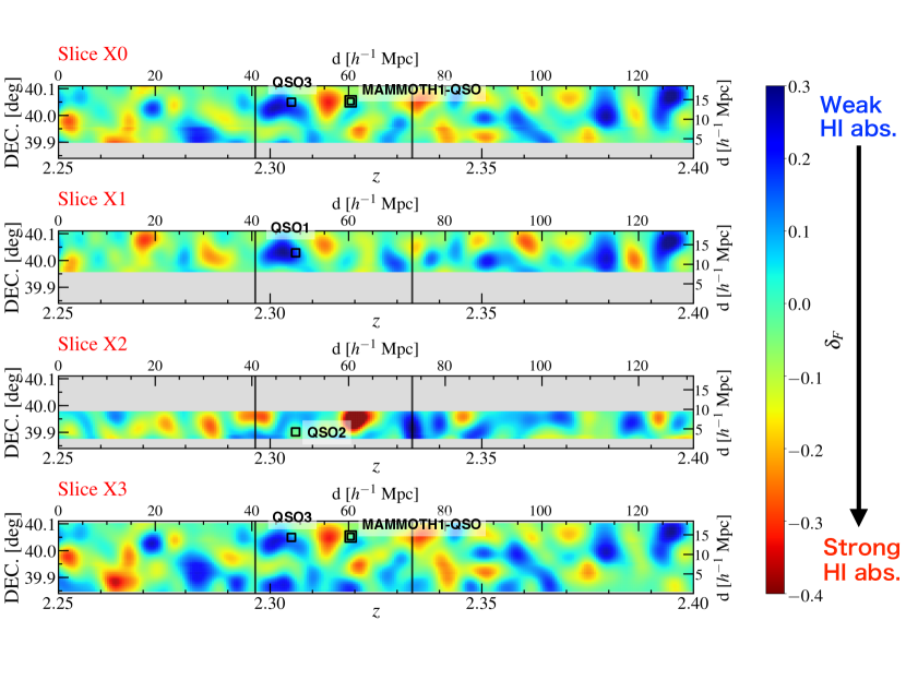
Figure 7: Projections of our Hi tomographic map across $2.6h^{-1}$ cMpc slices in the R.A. direction centered at the positions of MAMMOTH1-QSO and QSOs 1–3 from top to bottom. The projected R.A. ranges are shown in Figure 8. The color contours represent the Hi overdensity $\delta_{F}$ such that negative values (red) correspond to higher overdensities. The double square indicates the position of MAMMOTH1-QSO, and the single squares show QSOs 1–3. The two vertical lines at $z\simeq 2.30$ and $z\simeq 2.33$ denote the redshift range where Ly$\alpha$ emission can be probed with NB403 used in Cai et al. (2017a, b) (Section 4.3).

Note that there is a representative of Hi absorption measurements as a function of transverse distances to $z\sim 2$ type-I quasars performed by Prochaska et al. (2013), who have made use of a large ensemble of foreground/background quasar pairs based on the Quasar Probing Quasar survey (hereafter QPQ6). We estimate Hi absorption around MAMMOTH1-QSO and QSOs 1–3 with the same method as used in QPQ6, and present comparisons with the QPQ6 results in Appendix A. We could not investigate Hi gas distributions at small scales of $R_{\rm 3D}\lesssim 1$ pMpc where the QPQ6 study probes, because of the small number of background sightlines close to the quasars and thus the large uncertainties. The detailed comparison will be conducted with future dense sampling of background sightlines at small scales of $R_{\rm 3D}\lesssim 1$ pMpc.

4.3 LAE-HI overdensity

As described in Section 1, the LAE overdense region has been found around MAMMOTH1-QSO in previous narrowband (NB403) imaging observations (Cai et al., 2017b). Since galaxies are good tracers of LSSs of the matter distribution in the universe, it is interesting to compare the spatial distribution of LAE overdensities with that of Hi overdensities.

We compute the LAE overdensity based on the LAE sample constructed by Cai et al. (2017b). The LAE overdensity $\delta_{\rm LAE}$ is defined as

$$\delta_{\rm LAE}\equiv\frac{n_{\rm LAE}}{\overline{n}_{\rm LAE}}-1,$$ (5)

where $n_{\rm LAE}$ and $\overline{n}_{\rm LAE}$ are the LAE number density and its average, respectively, measured in a cylinder with a radius of $\langle d_{\perp}\rangle\simeq 2.6\ h^{-1}$ cMpc. For the cylinder length along the $z$ direction, we adopt a length of $\simeq 32.4h^{-1}$ cMpc that corresponds to the redshift range where Ly$\alpha$ emission can be detected within the FWHM of NB403, i.e, $z=2.30$–$2.33$. The obtained LAE overdensity is presented in Figure 1. We find two LAE LSSs whose density peaks are located at (R.A., Decl.) $=$ (14:41:27.12, +40:02:00.6) and (14:41:07840, +39:55:22.8).

In Figure 8, we compare the sky distribution of the LAE overdensity with the projected Hi overdensity over the same redshift range of $z=2.30$–$2.33$ calculated from the Hi tomographic map. We find that the two LAE density peaks are spatially offset from the Hi density peaks by $\sim 3-5h^{-1}$ cMpc. It is thought that galaxies are good tracers of underlying gas and dark matter distributions. However, since LAEs are star-forming galaxies and can emit ionizing photons, the Hi gas near the LAE density peaks would be relatively easily photo-ionized compared to LAE underdense regions. Such an anisotropic ionizing background radiation created by the density fluctuations of star-forming galaxies may cause this segregation between LAEs and Hi LSSs.

Another interesting point in Figure 8 is that the two LAE overdense structures are bridged by one of the Hi overdense structures. This would be consistent with the picture that galaxy overdense structures are connected by the Hi cosmic web.

We also find that the position of MAMMOTH-1 is located around the edges of the LAE overdense region and the Hi overdense region. In previous studies, LAEs with extended Ly$\alpha$ emission at similar redshifts tend to locate around the edges of galaxy overdense regions rather than the density peaks (Bădescu et al., 2017; Mawatari et al., 2012). Our results are consistent with these previous results.

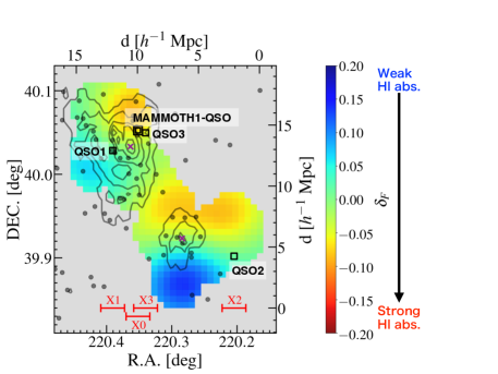
Figure 8: Projection of the Hi tomographic map over the redshift range of $z=2.30$–$2.33$. The color contours represent the projected $\delta_{F}$. The gray dots are the LAEs found by Cai et al. (2017b) and the gray contours represent the significances of the LAE overdensities from $2\sigma$ to $6\sigma$. The LAE distribution shows two density peaks that are marked with purple crosses. The double square indicates the position of MAMMOTH1-QSO and the single squares are those of the three neighboring type-I quasars. The red bars X0–X3 correspond to the R.A. ranges adopted for the slices in Figure 7.

5 Conclusion

We have investigated the 3D distribution of IGM Hi gas around the ELAN of MAMMOTH-1 at $z=2.3$. In a volume of $16\times 19\times 131\ h^{-3}{\rm cMpc}^{3}$ around MAMMOTH1-QSO, we have constructed an Hi tomographic map based on Ly$\alpha$ forest absorption detected in one eBOSS quasar and 16 Keck/LRIS galaxy spectra. By combining the Hi tomographic map results with Hi overdensity estimates based on background quasar spectra in the outer region, we have derived a spherically averaged Hi radial profile of MAMMOTH1-QSO over a wide range of scales from about $0.1$ pMpc to $100$ pMpc. Our results are summarized below.

1. The IGM Hi tomographic map reveals the existence of Hi overdense ($\delta_{F}\simeq-0.3-(-0.2)$) and underdense ($\delta_{F}\simeq 0.3-0.2$) LSSs with the size of $10-20\ h^{-1}{\rm cMpc}$ for the first time, indicating that the Hi gas distribution around MAMMOTH1-QSO is inhomogeneous.

2. The Hi radial profile of MAMMOTH1-QSO has a possible turnover at $R_{\rm 3D}\simeq 3$ pMpc and may increase with decreasing $R_{\rm 3D}$, suggesting that MAMMOTH1-QSO may have a proximity zone where the quasar photo-ionizes the surrounding Hi gas and suppresses Hi absorption. The MAMMOTH-1 Ly$\alpha$ nebula is probably a photo-ionized cloud embedded in the cosmic web.

3. The Hi radial profile of MAMMOTH1-QSO, which is a type-II quasar, is similar to those of neighboring three type-I quasars at similar redshifts. This result suggests that spherically averaged Hi gas distributions around type-I and type-II quasars are similar, which is compatible with the AGN unification model.

4. Based on a comparison between the Hi overdensity map and the distribution of LAEs around MAMMOTH1-QSO, we have found that their density peaks are spatially offset by about $3$–$5h^{-1}$ cMpc. This spatial offset between the Hi and LAE LSSs may reflect anisotropic UV background radiation created by star-forming galaxy density fluctuations in this field.

The connection between IGM Hi and galaxy formation in LSSs can be systematically explored by a wide-field spectroscopic survey of the Hobby-Eberly Telescope Dark Energy Experiment (HETDEX; Hill & HETDEX Consortium, 2016). The HETDEX survey will provide $10^{6}$ LAEs at $z\sim 2-3$ over $400$ deg², and reveal a number of extended Ly$\alpha$ nebulae and LSSs such as overdensities and filaments. The LSS/IGM study with HETDEX will be complementary to the ongoing program of CLAMATO (Lee et al., 2018), MAMMOTH (Cai et al., 2016), and the planned program of gigantic IGM tomographic mapping with Subaru/PFS (K. Nagamine et al. in prep.).

Appendix A Hi absorption as a function of transverse distances

In this Appendix, we estimate Hi absorption around MAMMOTH1-QSO and QSOs 1–3, and compare with the QPQ6 results (Prochaska et al., 2013). We use our background source spectra, and apply the same method as used in QPQ6 (hereafter $R_{\rm 2D}$ measurements) in which we take average of Hi absorption in a $\pm 1000$ km s^-1 velocity window around the QSOs as a function of transverse distances to the quasars ($R_{\rm 2D}$). The results for MAMMOTH1-QSO and QSOs 1–3 are shown in Figure 9. We find that our Hi absorption estimates are largely consistent with the QPQ6 result at $R_{\rm 2D}>0.6$ pMpc ($=1.3$ $h^{-1}$ cMpc) that corresponds to half the mean transverse sightline separation ${\langle d}_{\perp}\rangle$. We could not probe at $R_{\rm 2D}<0.6$ pMpc because of the small number of background sightlines close to the quasars and thus the large uncertainties. In Figure 9, we also show our Hi radial profiles (Section 3.2) to compare with the $R_{\rm 2D}$ measurements. We should be cautious about this comparison, because the $R_{\rm 2D}$ measurements probe the Hi absorption only in the transverse directions to the quasars while the Hi radial profiles are calculated with spherically averaged Hi overdensities, allowing us to probe the Hi radial profile averaged over all directions. Nevertheless, we find the possible turnovers at $\simeq 3$ pMpc in both the measurements, which could support our argument of proximity zones in Section 3.2. Since the data points of the Hi radial profiles below $0.6$ pMpc can be affected by interpolation in the tomographic reconstruction processes, these data are not well robust and we cannot directly compare with the QPQ6 results (See the caveat of the interpolation in Section 3.2). The detailed comparison will be conducted with future dense sampling of background sightlines.

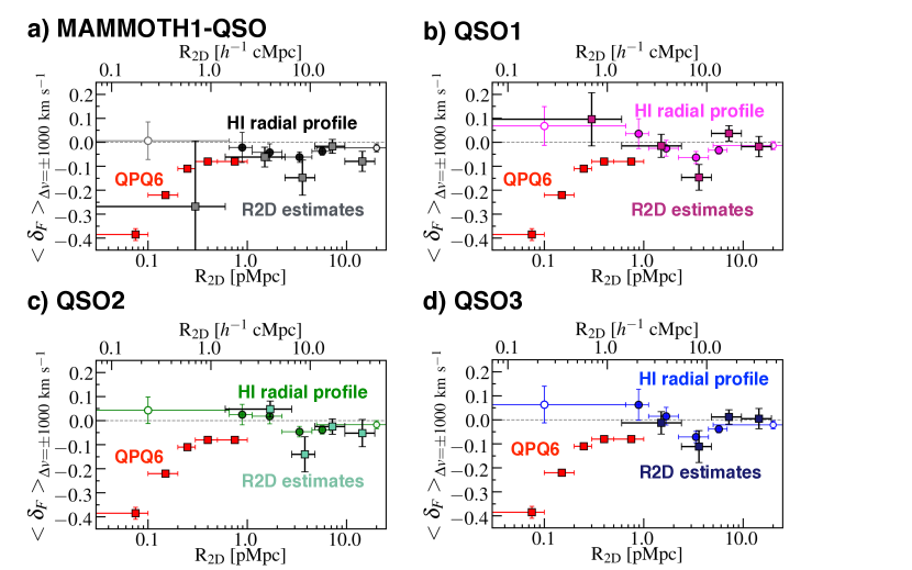
Figure 9: Hi absorption around MAMMOTH1-QSO and QSOs 1–3 estimated with the $R_{\rm 2D}$ measurements. The (gray, deeppink, lightgreen, navy) squares are $R_{\rm 2D}$ measurements around (MAMMOTH1-QSO, QSO1, QSO2, QSO3) in the BQ1 and BQ2 regions. Red squares are the results of QPQ6 (Prochaska et al., 2013). The (black, magenta, green, blue) circles are Hi radial profiles of (MAMMOTH1-QSO, QSO1, QSO2, QSO3) shown in Figures 5 and 6. The horizontal dotted line represents the cosmic average of the Hi absorption at $z=2.32$.

References

- Antonucci (1993) Antonucci, R. 1993, ARA&A, 31, 473
- Becker et al. (2013) Becker, G. D., Hewett, P. C., Worseck, G., & Prochaska, J. X. 2013, MNRAS, 430, 2067
- Berry et al. (2012) Berry, M., Gawiser, E., Guaita, L., et al. 2012, ApJ, 749, 4
- Bertin & Arnouts (1996) Bertin, E., & Arnouts, S. 1996, A&AS, 117, 393
- Brammer et al. (2008) Brammer, G. B., van Dokkum, P. G., & Coppi, P. 2008, ApJ, 686, 1503
- Bruzual & Charlot (2003) Bruzual, G., & Charlot, S. 2003, MNRAS, 344, 1000
- Bădescu et al. (2017) Bădescu, T., Yang, Y., Bertoldi, F., et al. 2017, ApJ, 845, 172
- Cai et al. (2016) Cai, Z., Fan, X., Peirani, S., et al. 2016, ApJ, 833, 135
- Cai et al. (2017a) Cai, Z., Fan, X., Yang, Y., et al. 2017a, ApJ, 837, 71
- Cai et al. (2017b) Cai, Z., Fan, X., Bian, F., et al. 2017b, ApJ, 839, 131
- Cai et al. (2019) Cai, Z., Cantalupo, S., Prochaska, J. X., et al. 2019, ApJS, 245, 23
- Calzetti et al. (2000) Calzetti, D., Armus, L., Bohlin, R. C., et al. 2000, ApJ, 533, 682
- Cantalupo et al. (2014) Cantalupo, S., Arrigoni-Battaia, F., Prochaska, J. X., Hennawi, J. F., & Madau, P. 2014, Nature, 506, 63
- Cantalupo et al. (2012) Cantalupo, S., Lilly, S. J., & Haehnelt, M. G. 2012, MNRAS, 425, 1992
- Casali et al. (2007) Casali, M., Adamson, A., Alves de Oliveira, C., et al. 2007, A&A, 467, 777
- Chabrier (2003) Chabrier, G. 2003, PASP, 115, 763
- Ciardullo et al. (2012) Ciardullo, R., Gronwall, C., Wolf, C., et al. 2012, ApJ, 744, 110
- D’Odorico et al. (2008) D’Odorico, V., Bruscoli, M., Saitta, F., et al. 2008, MNRAS, 389, 1727
- Elvis (2000) Elvis, M. 2000, ApJ, 545, 63
- Faucher-Giguère et al. (2008) Faucher-Giguère, C.-A., Prochaska, J. X., Lidz, A., Hernquist, L., & Zaldarriaga, M. 2008, ApJ, 681, 831
- Hayashino et al. (2019) Hayashino, T., Inoue, A. K., Kousai, K., et al. 2019, MNRAS, 484, 5868
- Hill & HETDEX Consortium (2016) Hill, G. J., & HETDEX Consortium. 2016, in Astronomical Society of the Pacific Conference Series, Vol. 507, Multi-Object Spectroscopy in the Next Decade: Big Questions, Large Surveys, and Wide Fields, ed. I. Skillen, M. Barcells, & S. Trager, 393
- Hinshaw et al. (2013) Hinshaw, G., Larson, D., Komatsu, E., et al. 2013, ApJS, 208, 19
- Inoue et al. (2014) Inoue, A. K., Shimizu, I., Iwata, I., & Tanaka, M. 2014, MNRAS, 442, 1805
- Kikuta et al. (2019) Kikuta, S., Matsuda, Y., Cen, R., et al. 2019, PASJ, 71, L2
- Lee et al. (2014a) Lee, K.-G., Hennawi, J. F., White, M., Croft, R. A. C., & Ozbek, M. 2014a, ApJ, 788, 49
- Lee et al. (2012) Lee, K.-G., Suzuki, N., & Spergel, D. N. 2012, AJ, 143, 51
- Lee et al. (2013) Lee, K.-G., Bailey, S., Bartsch, L. E., et al. 2013, AJ, 145, 69
- Lee et al. (2014b) Lee, K.-G., Hennawi, J. F., Stark, C., et al. 2014b, ApJ, 795, L12
- Lee et al. (2016) Lee, K.-G., Hennawi, J. F., White, M., et al. 2016, ApJ, 817, 160
- Lee et al. (2018) Lee, K.-G., Krolewski, A., White, M., et al. 2018, ApJS, 237, 31
- Mawatari et al. (2012) Mawatari, K., Yamada, T., Nakamura, Y., Hayashino, T., & Matsuda, Y. 2012, ApJ, 759, 133
- Mawatari et al. (2017) Mawatari, K., Inoue, A. K., Yamada, T., et al. 2017, MNRAS, 467, 3951
- Mukae et al. (2017) Mukae, S., Ouchi, M., Kakiichi, K., et al. 2017, ApJ, 835, 281
- Myers et al. (2015) Myers, A. D., Palanque-Delabrouille, N., Prakash, A., et al. 2015, ApJS, 221, 27
- Noterdaeme et al. (2012) Noterdaeme, P., Petitjean, P., Carithers, W. C., et al. 2012, A&A, 547, L1
- Oke & Gunn (1983) Oke, J. B., & Gunn, J. E. 1983, ApJ, 266, 713
- Oke et al. (1995) Oke, J. B., Cohen, J. G., Carr, M., et al. 1995, PASP, 107, 375
- Pâris et al. (2017) Pâris, I., Petitjean, P., Ross, N. P., et al. 2017, A&A, 597, A79
- Pâris et al. (2018) Pâris, I., Petitjean, P., Aubourg, É., et al. 2018, A&A, 613, A51
- Pedichini et al. (2003) Pedichini, F., Giallongo, E., Ragazzoni, R., et al. 2003, in Proc. SPIE, Vol. 4841, Instrument Design and Performance for Optical/Infrared Ground-based Telescopes, ed. M. Iye & A. F. M. Moorwood, 815–826
- Pettini et al. (2001) Pettini, M., Shapley, A. E., Steidel, C. C., et al. 2001, ApJ, 554, 981
- Pettini et al. (2000) Pettini, M., Steidel, C. C., Adelberger, K. L., Dickinson, M., & Giavalisco, M. 2000, ApJ, 528, 96
- Prochaska et al. (2013) Prochaska, J. X., Hennawi, J. F., Lee, K.-G., et al. 2013, ApJ, 776, 136
- Rakic et al. (2012) Rakic, O., Schaye, J., Steidel, C. C., & Rudie, G. C. 2012, ApJ, 751, 94
- Rudie et al. (2012) Rudie, G. C., Steidel, C. C., Trainor, R. F., et al. 2012, ApJ, 750, 67
- Shapley et al. (2003) Shapley, A. E., Steidel, C. C., Pettini, M., & Adelberger, K. L. 2003, ApJ, 588, 65
- Stark et al. (2015) Stark, C. W., White, M., Lee, K.-G., & Hennawi, J. F. 2015, MNRAS, 453, 311
- Suzuki et al. (2005) Suzuki, N., Tytler, D., Kirkman, D., O’Meara, J. M., & Lubin, D. 2005, ApJ, 618, 592
- Turner et al. (2014) Turner, M. L., Schaye, J., Steidel, C. C., Rudie, G. C., & Strom, A. L. 2014, MNRAS, 445, 794