Acoustokinetics: Crafting force landscapes from sound waves

Abstract

Factoring the pressure field of a harmonic sound wave into its amplitude and phase profiles provides the foundation for an analytical framework for studying acoustic forces that not only provides novel insights into the forces exerted by specified sound waves, but also addresses the inverse problem of designing sound waves to implement desired force landscapes. We illustrate the benefits of this acoustokinetic framework through case studies of purely nonconservative force fields, standing waves, pseudo-standing waves, and tractor beams.

I Introduction

Structured sound waves exert forces and torques that can be harnessed to transport, sort and organize insonated objects Zhang and Marston (2011); Wang et al. (2012); Marzo et al. (2015); Marzo and Drinkwater (2019). Applications include non-contact processing of sensitive Xie et al. (2006); Cao et al. (2012) and hazardous Andrade et al. (2016) materials, flow focusing for materials analysis and medical diagnostics Lenshof et al. (2012), and automated remote manipulation for research Courtney et al. (2013). Rapidly growing interest in harnessing acoustic forces has inspired a fundamental reassessment of the physics of wave-mediated forces. Recent developments in the theory of acoustic forces Bjerknes (1906); Blake Jr (1949); Gor’kov (1962); Settnes and Bruus (2012); Silva (2014) parallel the analogous theory of optical forces Gordon (1973); Chaumet and Nieto-Vesperinas (2000). Both offer valuable and often surprising insights into the elementary mechanisms of wave-matter interactions. The acoustokinetic framework introduced here addresses the complementary inverse problem: identifying what wave will create a desired force landscape.

The inverse problem for optical forces recently has been rendered more tractable by expressing the electromagnetic field in terms of its real-valued amplitudes and phases along each Cartesian coordinate Ruffner and Grier (2013); Yevick et al. (2016). This approach is called the theory of photokinetic effects and yields useful analytic expressions for the performance of optical traps Yevick et al. (2017) including design criteria for optical tractor beams Yevick et al. (2016). Here, we show that an analogous factorization of the pressure field in sound waves is similarly useful for understanding and implementing acoustic manipulation. We illustrate the utility of this acoustokinetic framework through case studies on nonconservative acoustic force fields, standing and pseudo-standing waves, and acoustic tractor beams.

I.1 Light: Photokinetic analysis

We develop acoustokinetics by analogy to photokinetics and therefore briefly review the theory of optical forces. A small particle immersed in an electromagnetic wave develops an electric dipole moment proportional to the local field. This induced dipole experiences a time-averaged Lorentz force in gradients of the field that can be expressed as Chaumet and Nieto-Vesperinas (2000)

$$\mathbf{F}_{e}(\mathbf{r})=\frac{1}{2}\Re\left\{\alpha_{e}\sum_{j=1}^{3}E_{j}(\mathbf{r})\nabla E_{j}^{\ast}(\mathbf{r})\right\},$$ (1)

where $E_{j}(\mathbf{r})$ is the $j$-th Cartesian coordinate of the electric field and $\alpha_{e}$ is the particle’s complex dipole polarizability. Expressing the components of the electric field in terms of their real-valued amplitude and phase profiles,

$$E_{j}(\mathbf{r})=u_{j}(\mathbf{r})\,e^{i\varphi_{j}(\mathbf{r})},$$ (2)

yields the surprisingly simple expression Ruffner and Grier (2013),

$$\mathbf{F}_{e}(\mathbf{r})=\frac{1}{4}\alpha_{e}^{\prime}\nabla\sum_{j=1}^{3}u_{j}^{2}(\mathbf{r})+\frac{1}{2}\alpha_{e}^{\prime\prime}\sum_{j=1}^{3}u_{j}^{2}(\mathbf{r})\nabla\varphi_{j}(\mathbf{r}),$$ (3)

where $\alpha_{e}^{\prime}$ and $\alpha_{e}^{\prime\prime}$ are the real and imaginary parts of the polarizability, respectively.

The first term on the right-hand side of Eq. (3) is the manifestly conservative intensity-gradient force responsible for single-beam optical traps such as optical tweezers Ashkin et al. (1986). The second describes a nonconservative force Wu et al. (2009) that is directed by phase gradients Roichman et al. (2008). Phase-gradient forces tend to drive trapped particles out of thermodynamic equilibrium with their supporting media Roichman et al. (2008); Sun et al. (2009), mediate the transfer of light’s orbital angular momentum Allen et al. (1992); He et al. (1995); Gahagan and Swartzlander (1996); Simpson et al. (1996), and have been used to create light-driven micromachines such as pumps Ladavac et al. (2004), mixers Ladavac and Grier (2005) and optical tractor beams Lee et al. (2010). Even non-absorbing dielectric particles experience nonconservative optical forces because of radiative contributions to the dipole polarizability Draine (1988); Albaladejo et al. (2010).

The dipole-order expression in Eq. (3) accurately describes the forces experienced by particles with radii, $a_{p}$, that are small enough to satisfy the Rayleigh criterion, $ka_{p}<1$, where $k$ is the wavenumber of light. In the Rayleigh regime, the conservative intensity-gradient force generally dominates the light-matter interaction because $\alpha_{e}^{\prime}$ scales as $(ka_{p})^{3}$, whereas $\alpha_{e}^{\prime\prime}$ scales as $(ka_{p})^{6}$.

I.2 Sound: Acoustic radiation forces

The analogous dipole-order acoustic radiation force experienced by a small particle in a harmonic sound field may be expressed in terms of the pressure, $p(\mathbf{r},t)$, as Silva (2014)

$$\mathbf{F}(\mathbf{r})=\frac{1}{2}\Re\left\{\alpha_{a}p\nabla p^{\ast}+\beta_{a}k^{-2}(\nabla p\cdot\nabla)\nabla p^{\ast}\right\},$$ (4)

where the coefficients $\alpha_{a}$ and $\beta_{a}$ play the role of dipole and quadrupole polarizabilities, respectively. This expression is analogous to Eq. (1) for optical forces and is obtained by rearranging terms from Eq. (16) in Ref. Silva (2014). It therefore also is equivalent Silva (2014) to the angular spectrum decomposition of $\mathbf{F}(\mathbf{r})$ Sapozhnikov and Bailey (2013) for $ka_{p}<1$. Expressing $\mathbf{F}(\mathbf{r})$ in terms of multipole polarizabilities clarifies the analogy with photokinetics. Lengths in Eq. (4) are scaled by the wavenumber, $k=\omega/c_{m}$, where $\omega$ is the sound’s frequency and $c_{m}$ is its speed in the medium. Equation (4) applies to inviscid fluids, for which the pressure satisfies the scalar wave equation

$$\nabla^{2}p=-k^{2}p.$$ (5)

Our focus on traveling waves in inviscid media is inspired by our interest in developing new modalities of long-ranged non-contact manipulation. Long-range manipulation is facilitated by minimizing acoustic losses in the medium. This can be achieved in air by working at frequencies below $50\text{\,}\mathrm{kHz}$ Marzo et al. (2015); Lim et al. (2019), for which the acoustic attenuation is less than $2\text{\,}\mathrm{dB}\text{\,}{\mathrm{m}}^{-1}$ under standard conditions Bass et al. (1995) and scales as $\omega^{2}$ for lower frequencies. The equivalent limiting frequency for water is roughly $2\text{\,}\mathrm{MHz}$ Ainslie and McColm (1998). Working at low frequencies also minimizes the influence of acoustic streaming forces, which ordinarily compete with acoustic radiation forces in viscous media and in inviscid media bounded by confining surfaces Lighthill (1978).

An object’s dipole and quadrupole polarizabilities generally depend on its size, shape and composition as well as the frequency of the sound and the properties of the fluid medium. For simplicity and concreteness, we will specialize to the case of a spherical scatterer of radius $a_{p}$ that is composed of a material of density $\rho_{p}$ and sound speed $c_{p}$. Such an object’s response to the sound field is characterized by the polarizabilities Silva (2014)

$$\alpha_{a} =\frac{4\pi a_{p}^{3}}{3\rho_{m}c_{m}^{2}}\,f_{0}\,\left[-1+i\frac{1}{3}(f_{0}+f_{1})(ka_{p})^{3}\right]$$ (6a)

$$\beta_{a} =\frac{2\pi a_{p}^{3}}{\rho_{m}c_{m}^{2}}\,f_{1}\,\left[1+i\frac{1}{6}f_{1}(ka_{p})^{3}\right],$$ (6b)

where the monopole coupling coefficient,

$$f_{0}=1-\frac{\rho_{m}c_{m}^{2}}{\rho_{p}c_{p}^{2}},$$ (7a)

depends on the compressibility mismatch between the particle and the medium, and the dipole coupling coefficient,

$$f_{1}=2\frac{\rho_{p}-\rho_{m}}{2\rho_{p}+\rho_{m}},$$ (7b)

gauges the density mismatch. These expressions also are obtained by reorganizing coefficients from Eq. (16) of Ref. Silva (2014) and are valid for $ka_{p}<1$. They constitute the leading-order contributions for both the real parts of the polarizabilities, $\alpha_{a}^{\prime}$ and $\beta_{a}^{\prime}$, and also the imaginary parts, $\alpha_{a}^{\prime\prime}$ and $\beta_{a}^{\prime\prime}$.

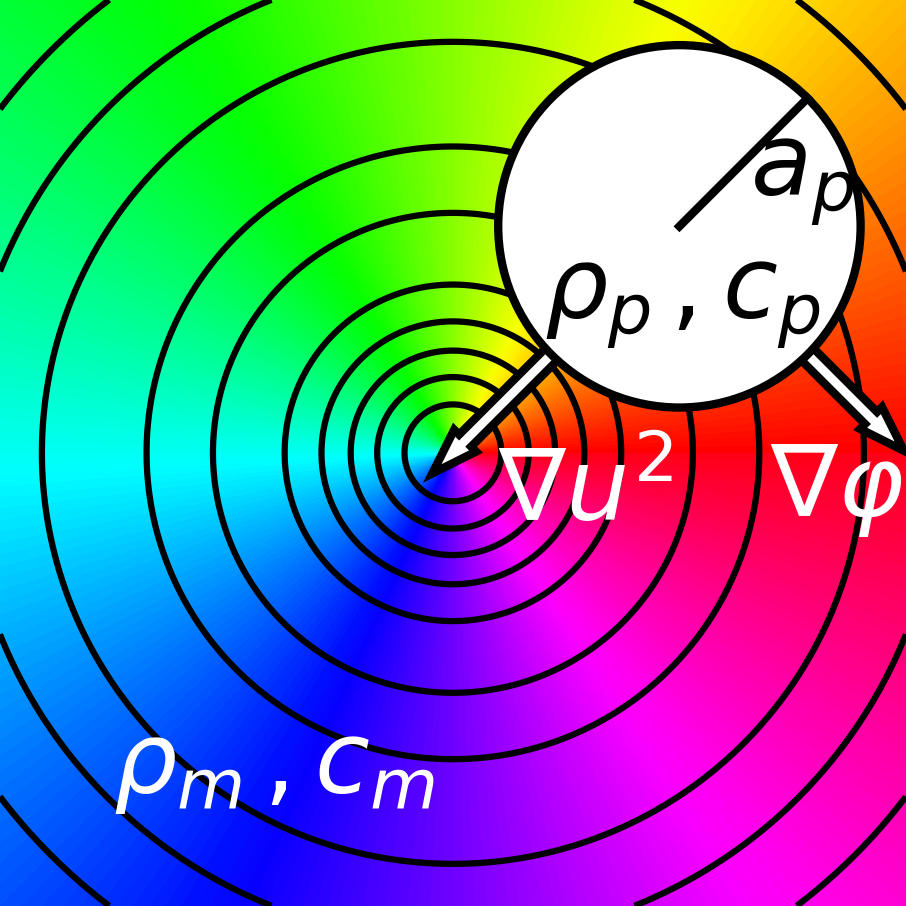
Figure 1: Schematic representation of a sphere of radius $a_{p}$ immersed in an acoustic pressure field. Contours denote isosurfaces of the pressure intensity. Colors represent the phase of the pressure field. Generally speaking, intensity gradients direct conservative trapping forces while phase gradients direct nonconservative driving forces.

II Acoustokinetic Framework

Drawing on the analogy with photokinetics, we express the harmonic sound wave’s pressure field in terms of its amplitude and phase profiles:

$$p(\mathbf{r},t)=u(\mathbf{r})\,e^{i\varphi(\mathbf{r})}\,e^{-i\omega t}.$$ (8)

The first term on the right-hand side of Eq. (4) then yields

$$\mathbf{F}_{\alpha}(\mathbf{r})=\frac{1}{4}\alpha_{a}^{\prime}\,\nabla u^{2}+\frac{1}{2}\alpha_{a}^{\prime\prime}\,u^{2}\nabla\varphi,$$ (9a)

which is directly analogous to Eq. (3) for the dipole-order force exerted by light. These contributions to the acoustic radiation force are depicted in Fig. 1. As in the optical case, $$\alpha_{a}^{\prime} \alpha_{a}^{\prime\prime} (ka_{p})^{3} (ka_{p})^{6}$$ and scale as and respectively, which means that the conservative force generally dominates for small particles.

The second term on the right-hand side of Eq. (4) arises from the velocity-matching condition at the sphere’s boundary and so has no analogue in optical radiation forces. It vanishes for density-matched particles ($\beta_{\alpha}=0$), which therefore behave exactly like dielectric particles in a light field, in agreement with conclusions from previous studies Toftul et al. (2019). When expressed in terms of the amplitude and phase profiles, this term separates naturally into a conservative contribution,

$$\mathbf{F}_{\beta}^{c}(\mathbf{r})=\frac{1}{4}\beta_{a}^{\prime}\nabla\left(u^{2}+\frac{1}{2}k^{-2}\nabla^{2}u^{2}\right),$$ (9b)

that augments the conservative intensity-gradient force from $\mathbf{F}_{\alpha}(\mathbf{r})$ and a nonconservative contribution,

$$\mathbf{F}_{\beta}^{nc}(\mathbf{r})=\frac{1}{4}\beta_{a}^{\prime\prime}k^{-2}\left[(2k^{2}u^{2}+\nabla^{2}u^{2}+2u\nabla u\cdot\nabla)\nabla\varphi\right.\\ \left.-(u\nabla^{2}\varphi+2u\nabla\varphi\cdot\nabla)\nabla u\right],$$ (9c)

that is directed both by phase gradients and also by amplitude gradients. The combination,

$$\mathbf{F}_{\beta}(\mathbf{r})=\mathbf{F}_{\beta}^{c}(\mathbf{r})+\mathbf{F}_{\beta}^{nc}(\mathbf{r}),$$ (9d)

captures the sphere’s leading-order coupling to the quadrupole components of the incident field. A derivation of Eq. (9) from Eq. (4) is presented in Appendix A.

Unlike the optical case, where quadrupolar forces generally are weaker than dipole contributions, the two terms in $\mathbf{F}_{\beta}(\mathbf{r})$ can be comparable in magnitude to their counterparts in $\mathbf{F}_{\alpha}(\mathbf{r})$ because $\beta_{a}^{\prime}$ scales as $(ka_{p})^{3}$ and $\beta_{a}^{\prime\prime}$ scales as $(ka_{p})^{6}$. These density-dependent terms therefore can be used to exert control in ways that are not possible with light.

For very small particles satisfying $ka_{p}\ll 1$, the acoustic force field is dominated by the conservative terms proportional to $\alpha_{a}^{\prime}$ and $\beta_{a}^{\prime}$. These terms are identical to the force described by the classic Gor’kov potential Gor’kov (1962), which is widely used to describe acoustic trapping phenomena Marzo et al. (2015); Bazou et al. (2012). For larger particles, and for appropriately structured sound fields, non-conservative contributions proportional to $\alpha_{a}^{\prime\prime}$ and $\beta_{a}^{\prime\prime}$ can be significant, and even can be dominant Melde et al. (2016); Démoré et al. (2014). Such contributions are not accounted for by the Gor’kov potential.

The acoustokinetic framework described by Eq. (9) is the principal contribution of this work. We now demonstrate its value through case studies on realizable sound fields with exceptional properties.

III Applications of the Acoustokinetic Framework

III.1 Designing purely nonconservative force fields

To illustrate how the acoustokinetic framework can address the inverse problem of designing sound waves to implement desired force landscapes, we use Eq. (9) to design harmonic sound waves that exert purely nonconservative forces. This is equivalent to requiring the conservative part of the acoustic radiation force to vanish, and thus requires us to look beyond the Gor’kov potential. Equations (9a) and (9b) show that this goal can be met if the particle is not density matched, $\beta_{a}^{\prime}\neq 0$, and if the pressure intensity satisfies the inhomogeneous Helmholtz equation,

$$\nabla^{2}u^{2}+2\left(1+\frac{\alpha_{a}^{\prime}}{\beta_{a}^{\prime}}\right)k^{2}\,u^{2}=C.$$ (10)

The undetermined constant $C$ distinguishes families of non-conservative sound waves for the class of objects with compatible values of $\alpha_{a}^{\prime}/\beta_{a}^{\prime}$. Solutions to Eq. (10) must be real-valued and must be paired with real-valued phase profiles that complete the description of the pressure field and satisfy the wave equation, Eq. (5).

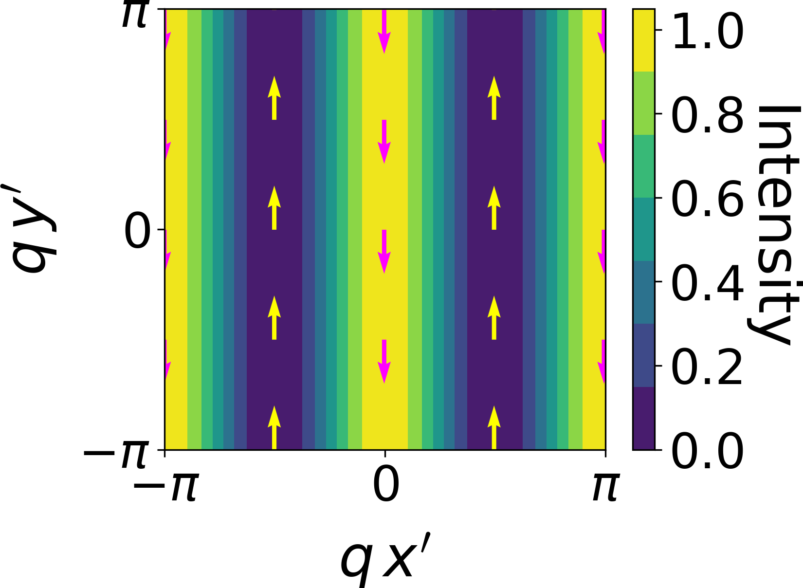
Figure 2: Intensity of the “picket fence” field in the $x^{\prime}y^{\prime}$-plane. For particularly selected parameters, the conservative force vanishes everywhere in this field, and the remaining force (indicated by arrows) is purely nonconservative. With the choice of material properties plotted ($C_{2}/C_{1}=1/3$), the direction of the force is also spatially modulated. The sign of the force in the $\hat{y}^{\prime}$ direction is also its sign in the $\hat{z}$ direction.

One interesting set of purely nonconservative solutions has the sinusoidal amplitude profile

$$u(\mathbf{r})=p_{0}\cos(q(x-y)),$$ (11a)

with spatial frequency

$$q=\frac{1}{2}\sqrt{1+\frac{\alpha_{a}^{\prime}}{\beta_{a}^{\prime}}}\,k.$$ (11b)

The associated phase profile,

$$\varphi(\mathbf{r})=kz\,\cos\gamma+(x+y)\sqrt{\frac{1}{2}k^{2}\sin^{2}\gamma-q^{2}},$$ (11c)

identifies this field as the superposition of two plane waves, each oriented at angle $$\gamma \hat{z}$$ relative to and at angle

$$\theta=\cos^{-1}\left(-\frac{\alpha_{a}^{\prime}}{\beta_{a}^{\prime}}\right)$$ (11d)

relative to one another in the $$(x,y)$$-plane.

Under these conditions, the in-plane component of the radiation pressure exactly cancels the conservative intensity-gradient force. The remaining scattering force is sinusoidally modulated in the transverse plane. The result is a “picket fence” of parallel force lines, which is illustrated in Fig. 2 using the rotated coordinates

$$x^{\prime} =x-y\quad\text{and}$$ (12a)

$$y^{\prime} =x+y$$ (12b)

for clarity. In these coordinates, the net force,

$$\mathbf{F}(\mathbf{r}^{\prime})=\frac{1}{4}kp_{0}^{2}\,f(x^{\prime})\,\hat{F},$$ (13a)

is directed along

$$\hat{F}=\sqrt{\frac{1}{2}\sin^{2}\gamma-\frac{q^{2}}{k^{2}}}\,\hat{y}^{\prime}+\cos\gamma\,\hat{z},$$ (13b)

and has an amplitude that varies with the transverse coordinate as

$$f(x^{\prime})=C_{1}+2(C_{2}-C_{1})\cos^{2}(qx^{\prime}).$$ (13c)

The scale and depth of the force landscape’s modulation depend on the object’s properties through $$C_{1}=\beta_{a}^{\prime\prime}(1+\alpha_{a}^{\prime}/\beta_{a}^{\prime}) C_{2}=\alpha_{a}^{\prime\prime}+\beta_{a}^{\prime\prime}$$ and .

Picket fence modes for a given type of object are distinguished by the angle of inclination, $\gamma$. The range of possible angles is limited by Eq. (11c) to

$$\sin^{2}\gamma>\frac{2q^{2}}{k^{2}}.$$ (14)

With this constraint, picket fences can be created for objects that satisfy

$$-1<\frac{\alpha_{a}^{\prime}}{\beta_{a}^{\prime}}<\sin^{2}\gamma.$$ (15)

Under some conditions, including those depicted in Fig. 2, the direction of the force can alternate within the fringe pattern. In terms of the standard coupling coefficients, alternating picket fences can be projected for objects satisfying

$$-\frac{3}{4}<\frac{f_{0}}{f_{1}}<-\frac{1}{2}.$$ (16)

Droplets of xylene hexafluoride ($\rho_{p}=$1370\text{\,}\mathrm{kg}\text{\,}{\mathrm{m}}^{-3}$$, $c_{p}=$880\text{\,}\mathrm{m}\text{\,}{\mathrm{s}}^{-1}$$) dispersed in butanol ($\rho_{m}=$810\text{\,}\mathrm{kg}\text{\,}{\mathrm{m}}^{-3}$$, $c_{m}=$1240\text{\,}\mathrm{m}\text{\,}{\mathrm{s}}^{-1}$$), for example, have $f_{0}/f_{1}=$-0.55$$ and thus are predicted to experience an alternating picket fence force field. Although alternating picket fences are only possible for a limited domain of material properties, picket fences in general could have practical applications for sorting objects by density or compressibility.

III.2 Conservative forces in standing waves

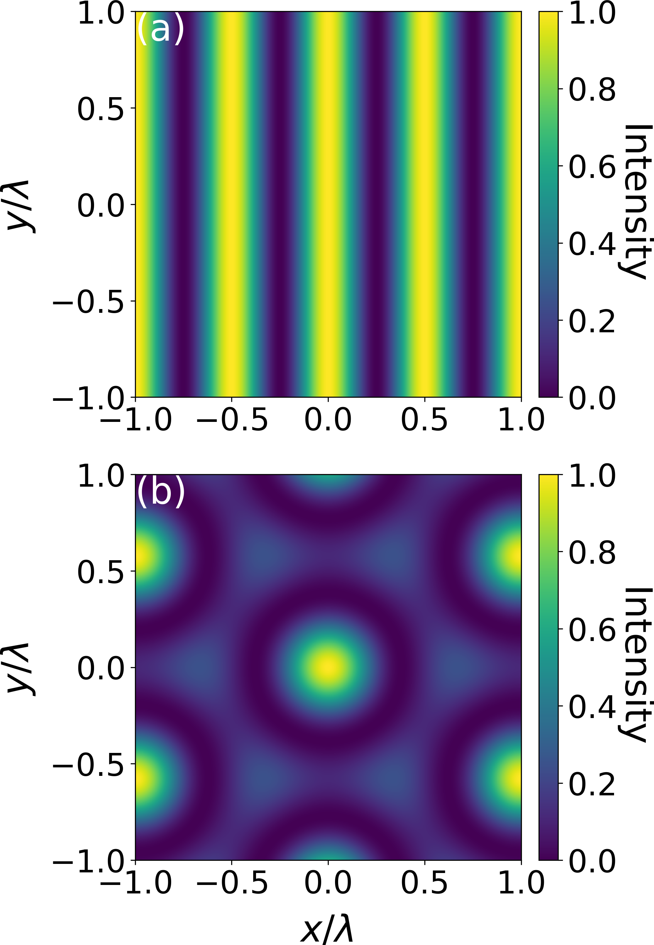
Figure 3: Maps of the pressure intensity of (a) a one-dimensional standing wave and (b) a sixfold standing wave. Particles are trapped either at intensity maxima or minima, depending on their composition relative to the medium.

The acoustokinetic framework also is useful for analyzing the force fields created by specified sound waves. Standing waves, for example, can be decomposed into superpositions of counterpropagating plane waves. The phase-dependent terms in $\mathbf{F}_{\alpha}(\mathbf{r})$ and $\mathbf{F}_{\beta}(\mathbf{r})$ vanish in such superpositions, leaving a manifestly conservative force landscape,

$$\mathbf{F}_{\text{standing}}(\mathbf{r})=\frac{1}{4}\nabla\left[\alpha_{a}^{\prime}u^{2}+\beta_{a}^{\prime}k^{-2}(\nabla u)^{2}\right].$$ (17)

Particles satisfying

$$\alpha_{a}^{\prime}-\beta_{a}^{\prime}>0$$ (18)

are drawn toward antinodes of the pressure field, as illustrated in Fig. 3. This condition is satisfied by compressible, low-density particles such as bubbles in water. Particles with complementary properties are drawn toward nodes.

III.3 Nonconservative forces in pseudo-standing waves

Not all zero-momentum waves are standing waves. Some have non-trivial phase profiles and so can exert nonconservative forces. The archetype for such pseudo-standing waves is a superposition of three plane waves with equal amplitude, $p_{0}/3$, and wave vectors

$$\mathbf{k}_{n}=-k\left[\cos\left(n\frac{2\pi}{3}\right)\,\hat{x}+\sin\left(n\frac{2\pi}{3}\right)\,\hat{y}\right]$$ (19)

that satisfy $\sum_{n=1}^{3}\mathbf{k}_{n}=0$ Masajada and Dubik (2001). The pressure intensity for such a three-wave superposition is plotted in Fig. 4(a) and displays a six-fold rotational symmetry similar to that of the corresponding six-fold standing wave in Fig. 3(b). The triangular lattice of antinodes in Fig. 4(a), however, is meshed with a dual hexagonal lattice of nodes, as indicated by dotted circles in Fig. 4(a). Because nonconservative forces tend to be weaker than conservative forces by a factor of $(ka_{p})^{3}$, we focus our attention on regions where the sound field forms stable traps, and expand about these points in polar coordinates, $\mathbf{r}=(r,\theta)$ for small displacements, $kr<1$.

For the three-fold pseudo-standing wave, the conservative contributions from Eqs. (9a) and (9b) simplify to

$$\mathbf{F}^{c}(\mathbf{r})=\frac{1}{8}\left(2\alpha_{a}^{\prime}-\beta_{a}^{\prime}\right)\nabla u^{2}.$$ (20)

Particles satisfying

$$2\alpha_{a}^{\prime}-\beta_{a}^{\prime}>0$$ (21)

therefore are drawn to pressure antinodes while complementary particles seek out nodes.

A node-seeking particle experiences amplitude and phase profiles of the form

$$u_{\text{node}}(\mathbf{r}) \approx\frac{1}{2}p_{0}\,kr\quad\text{and}$$ (22a)

$$\varphi_{\text{node}}(\mathbf{r}) \approx\pm\theta-\frac{\pi}{2}.$$ (22b)

The conservative part of the associated force field exerts a Hookean restoring force,

$$\mathbf{F}_{\text{node}}^{c}(\mathbf{r})\approx-\frac{1}{16}kp_{0}^{2}(\beta_{a}^{\prime}-2\alpha_{a}^{\prime})\,kr\,\hat{r},$$ (22c)

that keeps the particle localized near the node. The force field also includes a nonconservative component,

$$\mathbf{F}^{nc}_{\text{node}}(\mathbf{r})\approx\pm\frac{1}{8}kp_{0}^{2}(\alpha_{a}^{\prime\prime}+\beta_{a}^{\prime\prime})\,kr\,\hat{\theta},$$ (22d)

that is directed by the azimuthal phase gradient and causes the displaced particle to orbit its node. The pseudo-standing wave therefore transfers orbital angular momentum to particles moving near its nodes, with each node acting as a unit-charge acoustic vortex Zhang and Marston (2011). The sign of the orbital angular momentum alternates from site to site on the honeycomb lattice of nodes. The array of alternating acoustic vortexes in a pseudo-standing wave therefore carries no net angular momentum Bliokh and Nori (2019).

Nodes repel particles satisfying $2\alpha_{a}^{\prime}>\beta_{a}^{\prime}$, which instead seek out the triangular lattice of antinodes. Near an antinode, the sound field’s amplitude and phase profiles are

$$u_{\text{antinode}}(\mathbf{r}) \approx p_{0}\left[1-\frac{1}{4}(kr)^{2}\right]\quad\text{and}$$ (23a)

$$\varphi_{\text{antinode}}(\mathbf{r}) \approx\frac{1}{24}(kr)^{3}\,\cos 3\theta.$$ (23b)

For small displacements, the conservative terms from $$\mathbf{F}_{\alpha}(\mathbf{r}) \mathbf{F}_{\beta}(\mathbf{r})$$ and exert a Hookean restoring force on an antinode-seeking particle:

$$\mathbf{F}_{\text{antinode}}^{c}(\mathbf{r})=-\frac{1}{8}kp_{0}^{2}(2\alpha_{a}^{\prime}-\beta_{a}^{\prime})\,kr\,\hat{r}.$$ (23c)

The nonconservative terms create a sextupole flow that tends to drive the particle from one antinode to another:

$$\mathbf{F}_{\text{antinode}}^{nc}(\mathbf{r})=F_{0}\,k^{2}r^{2}(\cos 3\theta\,\hat{r}-\sin 3\theta\,\hat{\theta}),$$ (23d)

where $F_{0}=kp_{0}^{2}\,(2\alpha_{a}^{\prime\prime}-\beta_{a}^{\prime\prime})/32$.

The conservative part of the pseudo-standing wave’s force field vanishes for materials satisfying $2\alpha_{a}^{\prime}=\beta_{a}^{\prime}$, leaving a purely nonconservative force field. This contrasts with the force exerted by a standing wave, which is always conservative. Realizing this condition in practice, however, would require a precise balance of material properties.

More generally, systems satisfying $2\alpha_{a}^{\prime\prime}-\beta^{\prime\prime}_{a}>2\alpha_{a}^{\prime}-\beta_{a}^{\prime}$ will experience nonconservative forces that rival conservative trapping forces. In the particular case of an air bubble of size $ka_{p}=$0.3$$ in water, for example, the nonconservative force exceeds the conservative force for displacements greater than $kr\approx$0.025$$ from the pressure antinodes. A pseudo-standing wave at amplitude $p_{0}=$1\text{\,}\mathrm{kPa}$$ and frequency $f=\omega/(2\pi)=$2\text{\,}\mathrm{MHz}$$ yields a nonconservative force on the order of $1\text{\,}\mathrm{nN}$ for a displacement of $kr=$0.1$$ and a conservative force of just $0.1\text{\,}\mathrm{nN}$. The overall force field, being mostly nonconservative, resembles the streamlines in Fig. 4.

These observations illustrate that nonconservative forces can emerge along directions where the sound field carries no net momentum. More generally, it shows that radiation pressure can be directed independently of the direction of wave propagation. This independence can be used to craft tractor beams from propagation-invariant Bessel beams Marston (2006); Lee et al. (2010); Yevick et al. (2016).

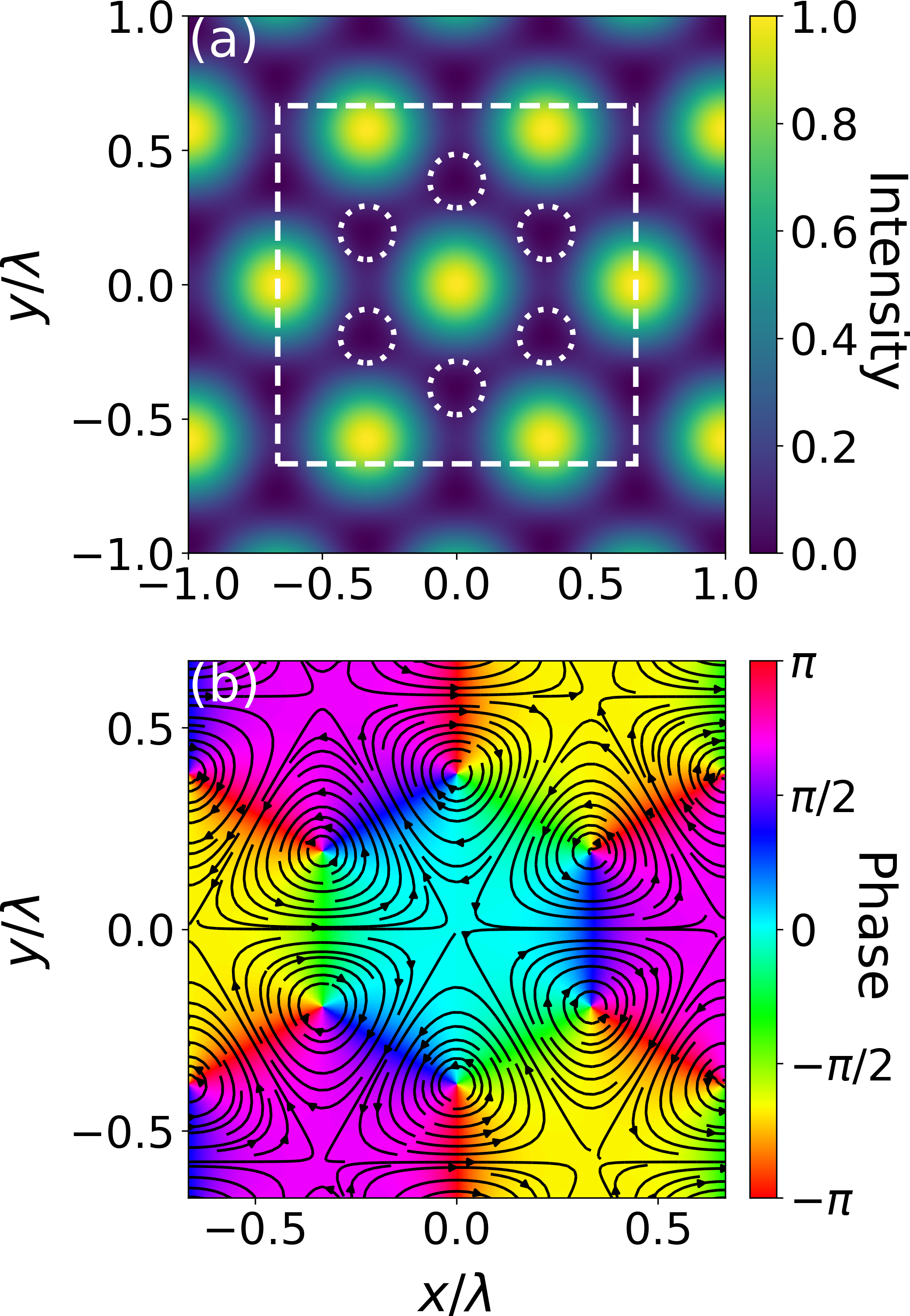
Figure 4: (a) Intensity and (b) phase maps of the threefold zero-momentum wave. Dashed white circles indicate the intensity nodes and phase singularities in the field, and the dashed white square indicates the region plotted in (b). Streamlines show the direction of the phase gradient, along which nonconservative forces act.

III.4 Bessel Beams and Tractor Beams

Both the standing wave and the pseudo-standing wave require boundary conditions that completely enclose their targets. Long-range manipulation without physical confinement is best achieved with propagation-invariant traveling waves. The natural basis for such applications is the family of Bessel beams Durnin (1987); Durnin et al. (1987); Marston (2006), which are non-diffracting solutions to Eq. (5) in cylindrical coordinates, $\mathbf{r}=(r,\theta,z)$. The amplitude and phase profiles for a Bessel beam propagating along $\hat{z}$ are

$$u_{\gamma,n}(\mathbf{r}) =p_{0}\,J_{n}(kr\sin\gamma)\quad\text{and}$$ (24)

$$\varphi_{\gamma,n}(\mathbf{r}) =kz\cos\gamma+n\theta,$$ (25)

respectively, where $J_{n}(\cdot)$ is a Bessel function of the first kind of order $n$. Bessel beams are distinguished by the convergence angle $\gamma$ that ranges from $\gamma=0$ for conventional plane waves to $\gamma=\pi/2$ for circular standing waves, and the integer $n$ that imposes a helical pitch on the beam’s wavefronts.

The conservative part of a Bessel beam’s force field is directed radially. Beams with $n=0$ have maximum intensity along the axis, $r=0$. Those with $n>0$ have zero intensity on the axis. The radial component of the acoustic force is linear in $kr$ for $\left|n\right|\leq 2$ and scales as $(kr)^{3}$, or higher, for $\left|n\right|>2$. Whether the force attracts the particle to the axis or repels it depends on the particle’s properties. For simplicity, we restrict our analysis to $\left|n\right|\leq 2$, in which case the conditions for particles to be trapped on-axis are

$$4\alpha_{a}^{\prime}+\beta_{a}^{\prime}\,(1+3\cos 2\gamma) >0, n =0$$ (26a)

$$\alpha_{a}^{\prime}+\beta_{a}^{\prime}\,\cos 2\gamma <0, n =\pm 1$$ (26b)

$$\beta_{a}^{\prime} <0, n =\pm 2.$$ (26c)

As noted recently Fan and Zhang (2019), the condition for stable trapping by an $n=0$ Bessel beam differs qualitatively from the analogous condition in Eq. (18) for trapping at an antinode of a standing wave. For example, dense objects with large values of $\beta_{a}^{\prime}$ are repelled by the antinodes of standing waves and pseudo-standing waves, but tend to be trapped by the central antinode of a Bessel beam with $\gamma<\pi/4$. Similar reversals arise for trapping at the central node of Bessel beams with $\left|n\right|>0$.

Having established the condition for stable transverse trapping, we next analyze the axial force on a particle localized at $r=0$. Any beam satisfying $\mathbf{F}(\mathbf{r})|_{r=0}\cdot\hat{z}<0$ can be said to act as a tractor beam. It should be noted that optical Bessel beams do not act as tractor beams for small objects because the dipole-order photokinetic force is always repulsive Yevick et al. (2016).

Axial forces in propagation-invariant Bessel beams are inherently nonconservative. The relevant terms in Eq. (9) yield

$$\mathbf{F}(\mathbf{r})|_{\begin{subarray}{c}n=0\\ r=0\end{subarray}} =\frac{1}{2}\left[(\alpha_{a}^{\prime\prime}+\beta_{a}^{\prime\prime})\,u^{2}+\frac{\beta_{a}^{\prime\prime}}{2k^{2}}\nabla^{2}u^{2}\right]\,\nabla\varphi$$ (27a)

$$=\frac{1}{2}\,p_{0}^{2}k\,(\alpha_{a}^{\prime\prime}+\beta_{a}^{\prime\prime}\,\cos^{2}\gamma)\,\cos\gamma\,\hat{z}.$$ (27b)

Unlike optical Bessel beams, therefore, acoustic Bessel beams can act as tractor beams for particles satisfying both the trapping condition from Eq. (26a) and also

$$\alpha_{a}^{\prime\prime}+\beta_{a}^{\prime\prime}\,\cos^{2}\gamma<0.$$ (28)

Expressed in terms of material properties, these conditions simplify to

$$f_{0}<\frac{3}{8}(1+3\cos 2\gamma)f_{1}\quad\text{and}$$ (29a)

$$\left(\frac{f_{0}}{f_{1}}\right)^{2}+\frac{f_{0}}{f_{1}}+\frac{3}{4}\cos^{2}\gamma<0.$$ (29b)

Figure 5 shows the domain of beam shapes and particle compositions for which the $n=0$ Bessel beam acts as a tractor beam. These include the optimal condition $f_{0}/f_{1}=-1/2$ that was identified in the original discussion of acoustic tractor beams Marston (2006).

Density-matched objects ($f_{1}=0$) can only be trapped if they are compressible enough that $f_{0}<0$. This means, however, that $\mathbf{F}\cdot\hat{z}>0$, from which we conclude that Bessel beams are not tractor beams for such objects. This is reflected in Fig. 5(b), which presents the axial pulling force as a function of the relative sound speed, $c_{m}/c_{p}$, and density, $\rho_{m}/\rho_{p}$ for a strongly converging Bessel beam with $\gamma=$$$.

For this convergence angle, the previously discussed system of xylene hexafluoride droplets immersed in butanol will experience a tractor force in the Rayleigh regime.

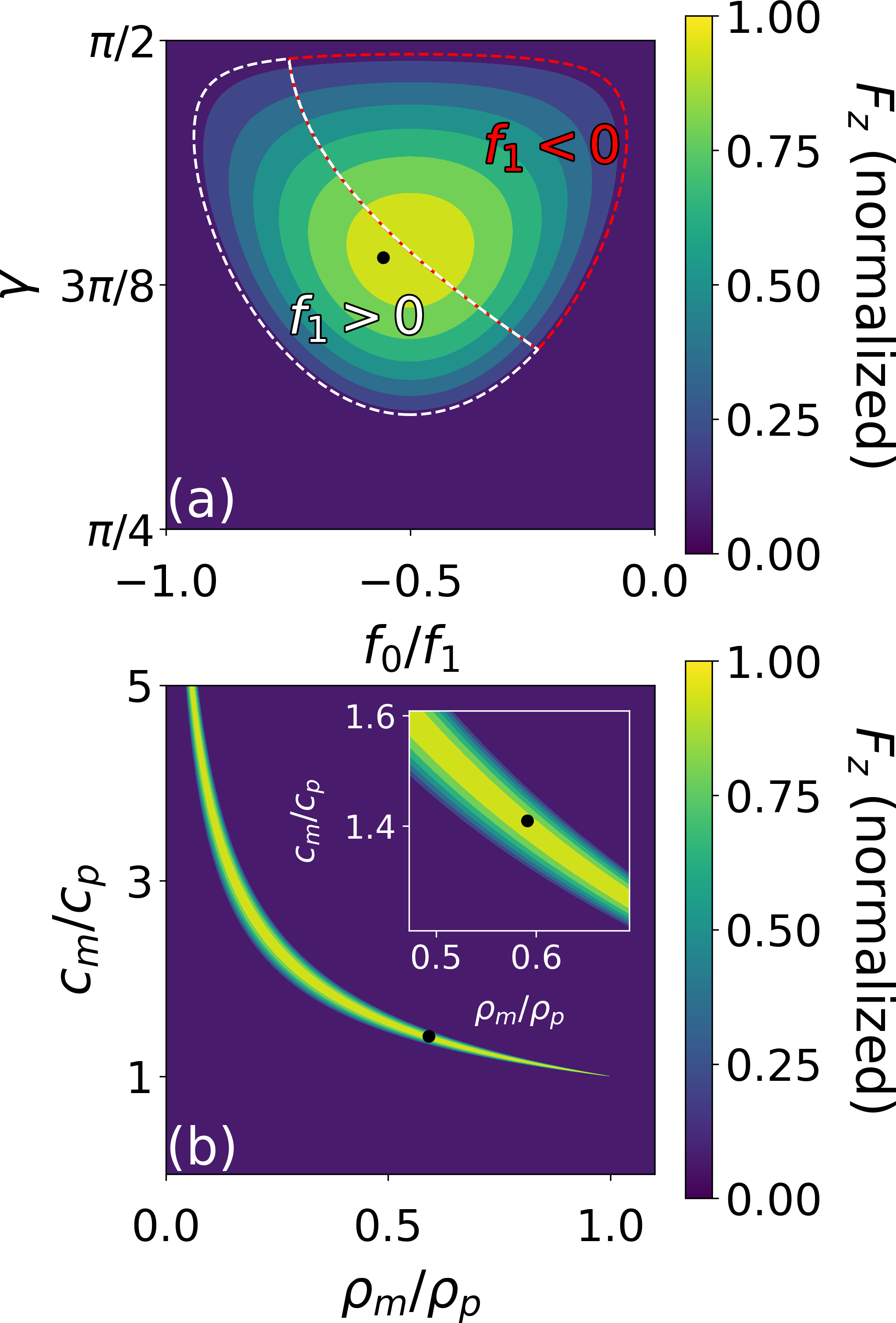
Figure 5: Relative strength of the axial force, $F_{z}\equiv\mathbf{F}(\mathbf{r})|_{r=0}\cdot\hat{z}$, acting on an object that is trapped along the axis of an $n=0$ Bessel beam. A value of 0 indicates that the object is not trapped on-axis. (a) Dense objects with $f_{1}>0$ are pulled upstream by the Bessel beam under conditions enclosed by the white curve and are repelled under complementary conditions enclosed by the red curve. These conditions are reversed for buoyant objects with $f_{1}<0$. Density-matched objects are always repelled. The Bessel beam acts like a tractor beam for all other objects along the interface between the red- and white-bordered regions. (b) The axial pulling force as a function of material parameters for the specific case $\gamma=$$$. The black point indicates parameters for droplets of the industrial solvent xylene hexafluoride in butanol. Inset: the region near this system.

The analogous treatment for $n=1$ yields

$$\mathbf{F}(\mathbf{r})|_{\begin{subarray}{c}n=1\\ r=0\end{subarray}} =\frac{\beta_{a}^{\prime\prime}}{4k^{2}}\,\nabla^{2}u^{2}\,\nabla\varphi$$ (30a)

$$=\frac{1}{4}p_{0}^{2}k\,\beta_{a}^{\prime\prime}\,\cos\gamma\sin^{2}\gamma\,\hat{z}.$$ (30b)

Because $\beta_{a}^{\prime\prime}>0$, such beams do act as tractor beams for any choice of materials, at least not for objects trapped on the axis. They instead drive trapped objects downstream.

The $n=2$ beam can trap small objects on the axis, but exerts no axial force at all,

$$\mathbf{F}(\mathbf{r})|_{\begin{subarray}{c}n=2\\ r=0\end{subarray}}=0.$$ (31)

Such beams might serve as useful conduits for Rayleigh particles that are moved back and forth along the axis by other forces.

IV Discussion

The theory of acoustokinetic forces presented here expresses the influence of a sound wave on a small object in terms of the amplitude and phase profiles of the pressure field. The resulting analytical framework, which is summarized in Eq. (9), offers a complementary perspective on acoustic forces to the standard development, which explicitly refers to the velocity field. Acoustokinetic expressions are particularly useful for designing acoustic force fields because they inherently account for coupling between the pressure and velocity fields and specify amplitude and phase profiles that can be controlled with transmissive, reflective or emissive elements.

The acoustokinetic approach yields expressions that closely resemble results for optical forces in the Rayleigh limit. Exploring the differences and similarities between acoustokinetic and photokinetic forces offers insights into how sound fields couple to material properties to generate useful and interesting force landscapes. The most important difference is that the particle’s polarizability includes contributions from the incident wave’s monopole component. This means that the force arising from the sound field’s dipole component includes terms at the same order of magnitude as leading quadrupole contributions. Such mixing does not arise in optical forces. It vanishes for objects that are density matched with the medium, yielding expressions for acoustic forces that are exactly analogous to their optical counterparts.

The acoustokinetic framework naturally accounts for the conservative nature of the force field exerted by standing waves and differentiates it from the influence of pseudo-standing waves that also carry no net momentum yet still exert nonconservative forces. When applied to acoustic Bessel beams, the acoustokinetic framework provides clear guidance on the limits for axial trapping and the conditions under which a zeroth-order Bessel beam can act as a tractor beam. This result contrasts with the equivalent analysis of optical Bessel beams, which do not act as tractor beams in the Rayleigh regime.

These examples illustrate the value of the acoustokinetic framework for analyzing acoustic force fields. More generally, the expressions from Eq. (9) can be solved either numerically, or in some cases analytically, for the phase and amplitude profiles that correspond to a specified force field acting on a particle of a given size, compressibility and density. As in the optical case, the framework can be extended beyond the dipole approximation. For objects substantially smaller than the wavelength of sound, however, the dipole-order terms are simple enough to yield analytical expressions. This framework also can be extended to handle interactions among insonated objects, an effect usually referred to as secondary Bjerknes forces.

V Acknowledgments

This work was supported by the MRSEC program of the National Science Foundation through Award Number DMR-1420073. The authors acknowledge helpful conversations with Phillip Marston (Washington State University) and Konstantin Bliokh (The Australian National University and RIKEN, Japan).

Appendix A Derivation of Equation (9)

The central idea of the acoustokinetic framework is to factor the incident pressure field $p(\mathbf{r})$ into its real-valued amplitude $u(\mathbf{r})$ and phase $\varphi(\mathbf{r})$:

$$p(\mathbf{r})=u(\mathbf{r})\,e^{i\varphi(\mathbf{r})}.$$ (32)

Expressed in these terms, the Helmholtz wave equation, Eq. (10), separates into two coupled differential equations that constrain the amplitude and phase profiles,

$$\nabla^{2}u+k^{2}u-u(\nabla\varphi)^{2}=0$$ (33a)

$$u\nabla^{2}\varphi+2\nabla u\cdot\nabla\varphi=0.$$ (33b)

These constraints transform the expression for the time-averaged acoustic force in Eq. (4) into the acoustokinetic expressions in Eq. (9).

The right-hand side of Eq. (4) is readily expanded into the sum of four terms

$$\mathbf{F}(\mathbf{r})=\frac{1}{2}\big{[} \quad\alpha_{a}^{\prime}\,\Re\{p\nabla p^{*}\}-\alpha_{a}^{\prime\prime}\,\Im\{p\nabla p^{*}\}$$ (34a)

$$+k^{-2}\beta_{a}^{\prime}\,\Re\{(\nabla p\cdot\nabla)\nabla p^{*}\}$$ (34b)

$$-k^{-2}\beta_{a}^{\prime\prime}\,\Im\{(\nabla p\cdot\nabla)\nabla p^{*}\}\big{]},$$ (34c)

each of will be expressed in terms of $u(\mathbf{r})$ and $\varphi(\mathbf{r})$. Substituting Eq. (32) into Eq. (34a) and noting that

$$p\nabla p^{*}=\frac{1}{2}\nabla u^{2}-iu^{2}\nabla\varphi$$ (35)

leads directly to Eq. (9a). The first term on the right-hand side of Eq. (35) is the gradient of an analytic function, and therefore corresponds to a manifestly conservative force. We demonstrate that the second term corresponds to a purely nonconservative force by showing that it is divergence-free:

$$\nabla\cdot(u^{2}\nabla\varphi) =\nabla(u^{2})\cdot\nabla\varphi+u^{2}\nabla^{2}\varphi$$ (36)

$$=2u\nabla u\cdot\nabla\varphi+u^{2}\nabla^{2}\varphi$$

$$=0,$$

with the last line following from Eq. (33b).

The expressions in Eqs. (34b) and (34c) depend on the real and imaginary parts of $(\nabla p\cdot\nabla)\nabla p^{*}$. The real part is conveniently transformed using the vector identity,

$$\nabla(\mathbf{A}\cdot\mathbf{B})=(\mathbf{A}\cdot\nabla)\mathbf{B}+(\mathbf{B}\cdot\nabla)\mathbf{A}\\ +\mathbf{A}\times(\nabla\times\mathbf{B})+\mathbf{B}\times(\nabla\times\mathbf{A}).$$ (37)

Setting $\mathbf{A}=\nabla p$ and $\mathbf{B}=\nabla p^{*}$ causes the curls on the right-hand side of Eq. (37) to vanish identically. The two remaining terms yield

$$\Re\{(\nabla p\cdot\nabla)\nabla p^{*}\} =\frac{1}{2}\nabla(\nabla p\cdot\nabla p^{*})$$ (38)

$$=\frac{1}{2}\nabla\left[(\nabla u)^{2}+u^{2}(\nabla\varphi)^{2}\right].$$ (39)

Combining this with Eq. (33a) and the identity $\nabla^{2}(u^{2})=2u\nabla^{2}u+2(\nabla u)^{2}$ yields Eq. (9b).

Equation (9c) similarly follows from the identity

$$\nabla\times(\mathbf{A}\times\mathbf{B})=\mathbf{A}(\nabla\cdot\mathbf{B})-\mathbf{B}(\nabla\cdot\mathbf{A})\\ +(\mathbf{B}\cdot\nabla)\mathbf{A}-(\mathbf{A}\cdot\nabla)\mathbf{B}.$$ (40)

Setting $\mathbf{A}=\nabla p$ and $\mathbf{B}=\nabla p^{*}$, we obtain

$$\Im\{(\nabla p\cdot\nabla)\nabla p^{*}\}=-\Im\{\nabla^{2}p\nabla p^{*}\}\\ +\frac{i}{2}\nabla\times(\nabla p\times\nabla p^{*}).$$ (41)

We use the Helmholtz equation to eliminate the Laplacian operator on the right-hand side so that

$$\Im\{\nabla^{2}p\nabla p^{*}\} =k^{2}\Im\{p\nabla p^{\ast}\}$$ (42)

$$=-k^{2}u^{2}\nabla\varphi,$$ (43)

with Eq. (43) following from Eq. (35). As before, this term is divergence-free and therefore corresponds to a purely non-conservative force.

The second term on the right-hand side of Eq. (41) is the curl of a function and thus also corresponds to a non-conservative force. It may be expressed in terms of the wave’s amplitude and phase profiles as

$$\frac{i}{2}\nabla\times(\nabla p\times\nabla p^{*})=\nabla\times\left[u(\nabla u\times\nabla\varphi)\right]\\ =u\nabla\times(\nabla u\times\nabla\varphi)+\nabla u\times(\nabla u\times\nabla\varphi)$$ (44)

The first term on the right-hand side of Eq. (44) can be rewritten as

$$u\nabla\times(\nabla u\times\nabla\varphi)=u(\nabla^{2}\varphi+\nabla\varphi\cdot\nabla)\nabla u\\ -u(\nabla^{2}u+\nabla u\cdot\nabla)\nabla\varphi,$$ (45)

while the second can be expressed as

$$\nabla u\times(\nabla u\times\nabla\varphi)=(\nabla u\cdot\nabla\varphi)\nabla u\\ -(\nabla u\cdot\nabla u)\nabla\varphi.$$ (46)

Using Eq. (33b) to eliminate $\nabla u\cdot\nabla\varphi$ and combining all remaining terms yields Eq.(9c).

References

- Zhang and Marston (2011) Likun Zhang and Philip L Marston, “Angular momentum flux of nonparaxial acoustic vortex beams and torques on axisymmetric objects,” Phys. Rev. E 84, 065601 (2011).
- Wang et al. (2012) Wei Wang, Luz Angelica Castro, Mauricio Hoyos, and Thomas E Mallouk, “Autonomous motion of metallic microrods propelled by ultrasound,” ACS Nano 6, 6122–6132 (2012).
- Marzo et al. (2015) Asier Marzo, Sue Ann Seah, Bruce W. Drinkwater, Deepak Ranjan Sahoo, Benjamin Long, and Sriram Subramanian, “Holographic acoustic elements for manipulation of levitated objects,” Nat. Commun. 6, 8661 (2015).
- Marzo and Drinkwater (2019) Asier Marzo and Bruce W. Drinkwater, “Holographic acoustic tweezers,” Proc. Natl. Acad. Sci. U.S.A. 116, 84–89 (2019).
- Xie et al. (2006) W. J. Xie, C. D. Cao, Y. J. Lü, Z. Y. Hong, and B. Wei, “Acoustic method for levitation of small living animals,” Appl. Phys. Lett. 89, 214102 (2006).
- Cao et al. (2012) Hui-Ling Cao, Da-Chuan Yin, Yun-Zhu Guo, Xiao-Liang Ma, Jin He, Wei-Hong Guo, Xu-Zhuo Xie, and Bo-Ru Zhou, “Rapid crystallization from acoustically levitated droplets,” J. Acoust. Soc. Am. 131, 3164–3172 (2012).
- Andrade et al. (2016) Marco A. B. Andrade, Anne L. Bernassau, and Julio C. Adamowski, “Acoustic levitation of a large solid sphere,” Appl. Phys. Lett. 109, 044101 (2016).
- Lenshof et al. (2012) Andreas Lenshof, Cecilia Magnusson, and Thomas Laurell, “Acoustofluidics 8: Applications of acoustophoresis in continuous flow microsystems,” Lab Chip 12, 1210–1223 (2012).
- Courtney et al. (2013) Charles RP Courtney, Bruce W Drinkwater, Christine EM Demore, Sandy Cochran, Alon Grinenko, and Paul D Wilcox, “Dexterous manipulation of microparticles using Bessel-function acoustic pressure fields,” Appl. Phys. Lett. 102, 123508 (2013).
- Bjerknes (1906) Vilhelm Bjerknes, Fields of Force (Columbia University Press, 1906).
- Blake Jr (1949) FG Blake Jr, “Bjerknes forces in stationary sound fields,” J. Acoust. Soc. Am. 21, 551–551 (1949).
- Gor’kov (1962) L. P. Gor’kov, “On the forces acting on a small particle in an acoustical field in an ideal fluid,” Sov. Phys. Dokl. 6, 773–775 (1962).
- Settnes and Bruus (2012) Mikkel Settnes and Henrik Bruus, “Forces acting on a small particle in an acoustical field in a viscous fluid,” Phys. Rev. E 85, 016327 (2012).
- Silva (2014) Glauber T. Silva, “Acoustic radiation force and torque on an absorbing compressible particle in an inviscid fluid,” J. Acoust. Soc. Am. 136, 2405–2413 (2014).
- Gordon (1973) James P. Gordon, “Radiation forces and momenta in dielectric media,” Phys. Rev. A 8, 14–21 (1973).
- Chaumet and Nieto-Vesperinas (2000) P. C. Chaumet and M. Nieto-Vesperinas, “Time-averaged total force on a dipolar sphere in an electromagnetic field,” Opt. Lett. 25, 1065–1067 (2000).
- Ruffner and Grier (2013) David B. Ruffner and David G. Grier, “Comment on ‘Scattering forces from the curl of the spin angular momentum of a light field’,” Phys. Rev. Lett. 111, 059301 (2013).
- Yevick et al. (2016) Aaron Yevick, David B. Ruffner, and David G. Grier, “Tractor beams in the Rayleigh limit,” Phys. Rev. A 93, 043807 (2016).
- Yevick et al. (2017) Aaron Yevick, Daniel J. Evans, and David G. Grier, “Photokinetic analysis of the forces and torques exerted by optical tweezers carrying angular momentum,” Phil. Trans. Roy. Soc. A 375, 20150432 (2017).
- Ashkin et al. (1986) A. Ashkin, J. M. Dziedzic, J. E. Bjorkholm, and S. Chu, “Observation of a single-beam gradient force optical trap for dielectric particles,” Opt. Lett. 11, 288–290 (1986).
- Wu et al. (2009) P. Y. Wu, R. X. Huang, C. Tischer, A. Jonas, and E. L. Florin, “Direct measurement of the nonconservative force field generated by optical tweezers,” Phys. Rev. Lett. 103, 108101 (2009).
- Roichman et al. (2008) Yohai Roichman, Bo Sun, Yael Roichman, Jesse Amato-Grill, and David G. Grier, “Optical forces arising from phase gradients,” Phys. Rev. Lett. 100, 013602 (2008).
- Sun et al. (2009) Bo Sun, Jiayi Lin, Ellis Darby, Alexander Y. Grosberg, and David G. Grier, “Brownian vortexes,” Phys. Rev. E 80, 010401(R) (2009).
- Allen et al. (1992) L. Allen, M. W. Beijersbergen, R. J. C. Spreeuw, and J. P. Woerdman, “Orbital angular-momentum of light and the transformation of Laguerre-Gaussian laser modes,” Phys. Rev. A 45, 8185–8189 (1992).
- He et al. (1995) H. He, M. E. J. Friese, N. R. Heckenberg, and H. Rubinsztein-Dunlop, “Direct observation of transfer of angular momentum to absorptive particles from a laser beam with a phase singularity,” Phys. Rev. Lett. 75, 826–829 (1995).
- Gahagan and Swartzlander (1996) K. T. Gahagan and G. A. Swartzlander, “Optical vortex trapping of particles,” Opt. Lett. 21, 827–829 (1996).
- Simpson et al. (1996) N. B. Simpson, L. Allen, and M. J. Padgett, “Optical tweezers and optical spanners with Laguerre-Gaussian modes,” J. Mod. Opt. 43, 2485–2491 (1996).
- Ladavac et al. (2004) Kosta Ladavac, Karen Kasza, and David G. Grier, “Sorting by periodic potential energy landscapes: Optical fractionation,” Phys. Rev. E 70, 010901(R) (2004).
- Ladavac and Grier (2005) Kosta Ladavac and David G. Grier, “Colloidal hydrodynamic coupling in concentric optical vortices,” Europhys. Lett. 70, 548–554 (2005).
- Lee et al. (2010) Sang-Hyuk Lee, Yohai Roichman, and David G. Grier, “Optical solenoid beams,” Opt. Express 18, 6988–6993 (2010).
- Draine (1988) B. T. Draine, “The discrete-dipole approximation and its application to interstellar graphite grains,” Astrophys. J. 333, 848–872 (1988).
- Albaladejo et al. (2010) S. Albaladejo, R. Gómez-Medina, L. S. Froufe-Pérez, H. Marinchio, R. Carminati, J. F. Torrado, G. Armelles, A. García-Martin, and J. J. Sáenz, “Radiative corrections to the polarizability tensor of an electrically small anisotropic dielectric particle,” Opt. Express 18, 3556–3567 (2010).
- Sapozhnikov and Bailey (2013) Oleg A Sapozhnikov and Michael R Bailey, “Radiation force of an arbitrary acoustic beam on an elastic sphere in a fluid,” J. Acoust. Soc. Am. 133, 661–676 (2013).
- Lim et al. (2019) Melody Xuan Lim, Kieran A Murphy, and Heinrich M Jaeger, “Edges control clustering in levitated granular matter,” arXiv preprint arXiv:1901.08656 (2019).
- Bass et al. (1995) Henry E. Bass, Louis C. Sutherland, Allen J. Zuckerwar, David T. Blackstock, and D. M. Hester, “Atmospheric absorption of sound: Further developments,” J. Acoust. Soc. Am. 97, 680–683 (1995).
- Ainslie and McColm (1998) Michael A. Ainslie and James G. McColm, “A simplified formula for viscous and chemical absorption in sea water,” J. Acoust. Soc. Am. 103, 1671–1672 (1998).
- Lighthill (1978) James Lighthill, “Acoustic streaming,” J. Sound Vibration 61, 391–418 (1978).
- Toftul et al. (2019) I. D. Toftul, K. Y. Bliokh, M. I. Petrov, and F. Nori, “Acoustic radiation force and torque on small particles as measures of the canonical momentum and spin densities,” arXiv preprint arXiv:1905.12216 (2019).
- Bazou et al. (2012) Despina Bazou, Angélica Castro, and Mauricio Hoyos, “Controlled cell aggregation in a pulsed acoustic field,” Ultrasonics 52, 842–850 (2012).
- Melde et al. (2016) Kai Melde, Andrew G. Mark, Tian Qiu, and Peer Fischer, “Holograms for acoustics,” Nature 537, 518 (2016).
- Démoré et al. (2014) Christine E. M. Démoré, Patrick M. Dahl, Zhengyi Yang, Peter Glynne-Jones, Andreas Melzer, Sandy Cochran, Michael P. MacDonald, and Gabriel C. Spalding, “Acoustic tractor beam,” Phys. Rev. Lett. 112, 174302 (2014).
- Masajada and Dubik (2001) Jan Masajada and Bogusława Dubik, “Optical vortex generation by three plane wave interference,” Opt. Commun. 198, 21–27 (2001).
- Bliokh and Nori (2019) Konstantin Y. Bliokh and Franco Nori, “Spin and orbital angular momenta of acoustic beams,” Phys. Rev. B 99, 174310 (2019).
- Marston (2006) Philip L. Marston, “Axial radiation force of a Bessel beam on a sphere and direction reversal of the force,” J. Acoust. Soc. Am. 120, 3518–3524 (2006).
- Durnin (1987) J. Durnin, “Exact-solutions for nondiffracting beams. 1. the scalar theory,” J. Opt. Soc. Am. A 4, 651–654 (1987).
- Durnin et al. (1987) J. Durnin, J. J. Miceli, Jr, and J. H. Eberly, “Diffraction-free beams,” Phys. Rev. Lett. 58, 1499–1501 (1987).
- Fan and Zhang (2019) Xu-Dong Fan and Likun Zhang, “Trapping force of acoustical Bessel beams on a sphere and stable tractor beams,” Phys. Rev. Appl. 11, 014055 (2019).