Abstract

We introduce the probabilistic sequential matrix factorization (PSMF) method for factorizing time-varying and non-stationary datasets consisting of high-dimensional time-series. In particular, we consider nonlinear Gaussian state-space models where sequential approximate inference results in the factorization of a data matrix into a dictionary and time-varying coefficients with potentially nonlinear Markovian dependencies. The assumed Markovian structure on the coefficients enables us to encode temporal dependencies into a low-dimensional feature space. The proposed inference method is solely based on an approximate extended Kalman filtering scheme, which makes the resulting method particularly efficient. PSMF can account for temporal nonlinearities and, more importantly, can be used to calibrate and estimate generic differentiable nonlinear subspace models. We also introduce a robust version of PSMF, called rPSMF, which uses Student-t filters to handle model misspecification. We show that PSMF can be used in multiple contexts: modeling time series with a periodic subspace, robustifying changepoint detection methods, and imputing missing data in several high-dimensional time-series, such as measurements of pollutants across London.

1 INTRODUCTION

The problem of $r$-rank factorization of a data matrix $Y\in{\mathbb{R}}^{d\times n}$ as

$$Y\approx CX$$ (1)

with $C\in{\mathbb{R}}^{d\times r}$ the dictionary matrix and $X\in{\mathbb{R}}^{r\times n}$ the coefficients, has received significant attention in past decades in multimedia signal processing and machine learning under the umbrella term of matrix factorization (MF) (Lee and Seung,, 1999, 2001; Mairal et al.,, 2010). The classical method for solving problems of the form (1) is nonnegative matrix factorization (NMF) (Lee and Seung,, 1999), which is proposed for nonnegative data matrices and obtains nonnegative factors. NMF and similar methods (e.g., singular value decomposition (SVD)) have been the focus of intensive research (Lin,, 2007; Berry et al.,, 2007; Ding et al.,, 2008; Cai et al.,, 2010; Févotte and Idier,, 2011) and has found applications in several fields, such as document clustering (Shahnaz et al.,, 2006), audio analysis (Smaragdis and Brown,, 2003; Ozerov and Févotte,, 2009), and video analysis (Bucak and Günsel,, 2009). This work was extended to general MF problems for real-valued data and factors, which found many applications including collaborative filtering (Rennie and Srebro,, 2005) and drug-target prediction (Zheng et al.,, 2013).

The problem in (1) was originally tackled from an optimization perspective, i.e., minimizing a cost $d(Y,CX)$ over $C$ and $X$ (Lee and Seung,, 1999, 2001; Lin,, 2007; Mairal et al.,, 2010). Another promising approach has been through a probabilistic model by defining priors on $C$ and $X$. This was explored by, e.g., Cemgil, (2009) with a Poisson-based model solved using variational inference (which reproduces NMF when the cost function is the Kullback-Leibler divergence) and in, e.g., Mnih and Salakhutdinov, (2008) and Salakhutdinov and Mnih, (2008) with a Gaussian model for the real-valued case solved via Markov chain Monte Carlo (MCMC). Naturally, online versions of these methods have received significant attention as they enable scaling up to larger datasets. On this front, a number of algorithms have been proposed that are based either on stochastic optimization (e.g., Bucak and Günsel,, 2009; Mairal et al.,, 2010; Gemulla et al.,, 2011; Mensch et al.,, 2016) or on a probabilistic model for online inference (Wang et al.,, 2012; Paisley et al.,, 2014; Akyildiz and Míguez,, 2019). However, these methods are generally for i.i.d. data and cannot exploit the case where the columns of $Y$ possess time dependency.

The success of MF in the i.i.d. data case motivated the development of matrix factorization methods for time-dependent data. In this case, the problem can be formulated as inferring parameters of a dynamical system or a state-space model (SSM), with a linear observation model $C$. This problem is also known as system identification (Katayama,, 2006). When the columns of $X$ (i.e. the hidden signal) also evolve linearly the problem reduces to that of inferring parameters of a linear SSM. This can be solved by maximum-likelihood estimation (MLE) through, e.g., expectation-maximization (EM) either offline (Ghahramani and Hinton,, 1996; Elliott and Krishnamurthy,, 1999) or online (Cappé and Moulines,, 2009; Cappé,, 2011), or with gradient-based methods (Andrieu et al.,, 2005; Kantas et al.,, 2015). In this vein, Yildirim et al., (2012) address the NMF problem by introducing a SSM with a Poisson likelihood where the inference is carried out with sequential Monte Carlo (SMC). In a similar manner Sun et al., (2012) propose an SSM-based approach where the dictionary is estimated using the EM algorithm. Similar MLE-based nonnegative schemes that also use SSMs attracted significant attention (e.g. Mohammadiha et al.,, 2013, 2014).

Although MLE estimates are consistent in the infinite data limit for general SSMs (Douc et al.,, 2011), EM-based methods are prone to get stuck in local minima (Katayama,, 2006) and provide only point estimates rather than full posterior distributions. As an alternative to the EM-based approaches, optimization-based methods were also explored (e.g. Boots et al.,, 2008; Karami et al.,, 2017; White et al.,, 2015) which again result in point estimates. If the transition model for the coefficients $X$ exhibits nonlinear dynamics while the observation model is linear (by the nature of MF), the problem reduces to parameter estimation in nonlinear SSMs (Särkkä,, 2013). The MLE approach is again prominent in this setting using EM or gradient methods (Kantas et al.,, 2015). However, when inference cannot be done analytically this results in the use of SMC (Doucet et al.,, 2000) or particle MCMC methods (Andrieu et al.,, 2010) (see Kantas et al., (2015) for an overview). Unfortunately, these methods suffer in the high-dimensional case (Bengtsson et al.,, 2008; Snyder et al.,, 2008) which makes Monte Carlo-based methods unsuitable for solving the MF problem. Optimization-based approaches that formulate a cost function with temporal regularizers have also been studied (e.g. Yu et al.,, 2016; Shi et al.,, 2016; Liu and Hauskrecht,, 2016; Ayed et al.,, 2019).

An alternative to the MLE or optimization-based approaches is to follow a Bayesian approach where a prior distribution is constructed over the parameters of the SSM, see, e.g., Särkkä, (2013). The goal is then to obtain the posterior distributions of the columns of $X$ and of $C$. This is also of interest when priors are used as regularizers to enforce useful properties such as sparsity (Cemgil,, 2009; Schmidt et al.,, 2009). In this context, an extension of the NMF-like decompositions to the dynamic setting was considered by Févotte et al., (2013), where the authors followed a maximum-a posteriori (MAP) approach. We refer to Févotte et al., (2018) for a literature review of temporal NMF methods. However, these methods are batch (offline) schemes and do not return a probability distribution over the dictionary or the coefficients. Joint posterior inference of $C$ and $X$ in a fully Bayesian setting is difficult as it usually requires sampling schemes (Salakhutdinov and Mnih,, 2008). To the best of our knowledge, a fully Bayesian approach for sequential (online) inference for matrix factorization that also scales well with the problem dimension has not been proposed in the literature.

Contribution.

In this work, we propose the probabilistic sequential matrix factorization (PSMF) method by framing our matrix factorization model as a nonlinear Gaussian SSM. Our formulation is fully probabilistic in the sense that we place a matrix-variate Gaussian prior on the dictionary and use a general Markov model for the evolution of the coefficients. We then derive a novel approximate inference procedure that is based on extended Kalman filtering (Kalman,, 1960; McLean et al.,, 1962) and results in a fast and efficient scheme. Our method is derived using numerical approximations to the optimal inference scheme and leverages highly efficient filtering techniques.

In particular, we derive analytical approximations and do not require a sampling procedure to approximate the posterior distributions. The inference method we provide is explicit and the update rules can be easily implemented without further consideration on the practitioner’s side. We also provide a robust extension of our model, called rPSMF, for the case where the model is misspecified and derive a corresponding inference scheme that adopts Student’s t-filters (Girón and Rojano,, 1994; Tronarp et al.,, 2019). Our methods can be easily tailored to the application at hand by modifying the subspace model, as the necessary derivatives can be easily computed through automatic differentiation.

This work is structured as follows. In Sec. 2 we introduce our probabilistic state-space model and the robust extension. Next we develop our tractable inference and estimation method in Sec. 3. In Sec. 4, our method is empirically evaluated in different scenarios such as learning structured subspaces, multivariate changepoint detection, and missing data imputation. Sec. 5 concludes the paper.

Notation

We denote the $d\times d$ identity matrix by $I_{d}$ and write ${\mathcal{N}}(x;\mu,\Sigma)$ for the Gaussian density over $x$ with mean $\mu$ and covariance matrix $\Sigma$. Similarly, ${\mathcal{T}}(x;\mu,\Sigma,\lambda)$ is the multivariate $t$ distribution with mean $\mu$, scale matrix $\Sigma$, and $\lambda$ degrees of freedom, and ${\mathcal{IG}}(s;\alpha,\beta)$ is the inverse gamma distribution over $s$ with shape and scale parameters $\alpha$ and $\beta$. Further, $\mathcal{MN}(X;M,U,V)$ denotes the matrix-variate Gaussian with mean-matrix $M$, row-covariance $U$, and column-covariance $V$. Sequences are written as $x_{1:n}=\{x_{1},\ldots,x_{n}\}$ and for a matrix $Z$, $z={\operatorname{vec}}(Z)$ denotes vectorization of $Z$. Recall that if $C\sim\mathcal{MN}(C;M,U,V)$, then $c\sim{\mathcal{N}}(c;{\operatorname{vec}}(M),V\otimes U)$ where $c={\operatorname{vec}}(C)$ and $\otimes$ the Kronecker product (Gupta and Nagar,, 1999). With $y_{k}$ and $x_{k}$ we respectively denote the $k$-th column of the matrices $Y$ and $X$.

2 THE PROBABILISTIC MODEL

We first describe the SSM, which consists of observations $(y_{k})_{k\geq 1}\in{\mathbb{R}}^{d}$, latent coefficients $(x_{k})_{k\geq 0}\in{\mathbb{R}}^{r}$, and a latent dictionary matrix $C\in{\mathbb{R}}^{d\times r}$, as follows

$$p(C) =\mathcal{MN}(C;C_{0},I_{d},V_{0}),$$ (2)

$$p(x_{0}) ={\mathcal{N}}(x_{0};\mu_{0},P_{0}),$$ (3)

$$p_{\theta}(x_{k}|x_{k-1}) ={\mathcal{N}}(x_{k};f_{\theta}(x_{k-1}),Q_{k}),$$ (4)

$$p(y_{k}|x_{k},C) ={\mathcal{N}}(y_{k};Cx_{k},R_{k}).$$ (5)

Here, $f_{\theta}\colon{\mathbb{R}}^{r}\times\Theta\to{\mathbb{R}}^{r}$ is a nonlinear mapping that defines the dynamics of the coefficients with $\Theta\subset{\mathbb{R}}^{d_{\theta}}$ the parameter space, and $(Q_{k},R_{k})_{k\geq 1}$ are respectively the noise covariances of the coefficient dynamics (4) and the observation model (5). The initial covariances of the coefficients and the dictionary are denoted by $P_{0}$ and $V_{0}$, respectively.

Intuitively, the model (2)–(5) is a dimensionality reduction model where the dynamical structure of the learned subspace is explicitly modeled via the transition density (4). This means that inferring $C$ and $(x_{k})_{k\geq 0}$ will lead to a probabilistic dimensionality reduction scheme where the dynamical structure in the data will manifest itself in the dynamics of the coefficients $(x_{k})_{k\geq 0}$. One main difficulty for applying standard schemes in this case is that we assume $C$ to be an unknown and random matrix, therefore, the (extended) Kalman filter cannot be applied directly for inference. To alleviate this problem, we formulate the prior in (2) with a Kronecker covariance structure, which enables us to update (conditional on $x_{k}$) the posterior distribution of $C$ analytically (Akyildiz and Míguez,, 2019).

2.1 The case of the misspecified model

In the model (2)–(5), when the practitioner does not have a good idea of how to set the hyperparameters or when they are misspecified, the resulting inference scheme may perform suboptimally. To remedy this situation and to demonstrate the flexibility of our framework, we additionally propose a robust version of our model by introducing an inverse-gamma-distributed scale variable, $s$, and the model

$$p(s) ={\mathcal{IG}}(s;\lambda_{0}/2,\lambda_{0}/2)$$ (6)

$$p(C\,|\,s) =\mathcal{MN}(C;C_{0},I_{d},sV_{0})),$$ (7)

$$p(x_{0}\,|\,s) ={\mathcal{N}}(x_{0};\mu_{0},sP_{0}),$$ (8)

$$p_{\theta}(x_{k}\,|\,x_{k-1},s) ={\mathcal{N}}(x_{k};f_{\theta}(x_{k-1}),sQ_{0}),$$ (9)

$$p(y_{k}\,|\,x_{k},C,s) ={\mathcal{N}}(y_{k};Cx_{k},sR_{0}),$$ (10)

Note that in this model only the initial noise covariances $Q_{0}$ and $R_{0}$ need to be specified, in contrast to the model in (2)–(5). By marginalizing out the scale variable $s$ in the multivariate normal distributions we obtain multivariate $t$ distributions (e.g., $p(x_{0})=\int{\mathcal{N}}(x_{0};\mu_{0},sP_{0}){\mathcal{IG}}(s;\lambda_{0}/2,\lambda_{0}/2)\,{\mathrm{d}}s={\mathcal{T}}(x_{0};\mu_{0},P_{0},\lambda_{0})$, see Bishop, (2006)). This technique has previously been used for robust versions of the Kalman filter (Girón and Rojano,, 1994; Basu and Das,, 1994; Roth et al.,, 2017, 2013; Tronarp et al.,, 2019). We follow the approach of Tronarp et al., (2019) to update $Q_{k}$ and $R_{k}$ at every iteration. These updates to the noise covariances lead to robustness in light of model misspecification, as discussed in Tronarp et al., (2019).

3 INFERENCE AND ESTIMATION

Here we derive the algorithm for performing sequential inference in the model (2)–(5). Inference in the robust model (6)–(10) is largely analogous, but necessary modifications are given in Sec. 3.2.3. We first present the optimal inference recursions and then describe our approximate inference scheme.

3.1 Optimal sequential inference

We give the optimal inference recursions for our model when $\theta$ is assumed to be fixed, and thus drop $\theta$ for notational clarity (parameter estimation is revisited in Sec. 3.2.4). To define a recursive one-step ahead procedure we assume that we are given the filters $p(x_{k-1}|y_{1:k-1})$ and $p(c|y_{1:k-1})$ at time $k-1$.

Prediction.

Using the model (2)–(5) we compute the predictive distribution as

$$p(x_{k}|y_{1:k-1})=\int p(x_{k-1}|y_{1:k-1})p(x_{k}|x_{k-1})\,{\mathrm{d}}x_{k-1}.$$ (11)

We note that given $p(x_{k-1}|y_{1:k-1})$ this step is independent of the dictionary.

Update.

Given this predictive distribution of $x_{k}$, we can now define the update steps of the method. In contrast to the Kalman filter, we have two quantities to update: $x_{k}$ and $c$. We first define the incremental marginal likelihood as

$$p(y_{k}|y_{1:k-1}) =\iint p(y_{k}|c,x_{k})p(x_{k}|y_{1:k-1})$$

$$\qquad\qquad p(c|y_{1:k-1})\,{\mathrm{d}}x_{k}\,{\mathrm{d}}c.$$ (12)

Next, we define the optimal recursions for updating the dictionary $C$ and coefficients $(x_{k})_{k\geq 1}$.
Dictionary Update: Given $p(y_{k}|y_{1:k-1})$, we can first update the dictionary as follows

$$p(c|y_{1:k})=p(c|y_{1:k-1})\frac{p(y_{k}|c,y_{1:k-1})}{p(y_{k}|y_{1:k-1})}$$ (13)

where

$$p(y_{k}|c,y_{1:k-1})=\int p(y_{k}|c,x_{k})p(x_{k}|y_{1:k-1})\,{\mathrm{d}}x_{k}.$$ (14)

Coefficient Update: We also update the coefficients at time $k$ (independent of the dictionary) as:

$$p(x_{k}|y_{1:k})=p(x_{k}|y_{1:k-1})\frac{p(y_{k}|x_{k},y_{1:k-1})}{p(y_{k}|y_{1:k-1})}$$ (15)

where

$$p(y_{k}|x_{k},y_{1:k-1})=\int p(y_{k}|x_{k},c)p(c|y_{1:k-1})\,{\mathrm{d}}c.$$ (16)

Unfortunately, these exact recursions are intractable. In the next section, we make these steps tractable by introducing approximations and obtain an efficient and explicit inference algorithm.

3.2 Approximate sequential inference

We start by assuming a special structure on the model. First, we note that the matrix-Gaussian prior in (2) can be written as $p(c)={\mathcal{N}}(c;c_{0},V_{0}\otimes I_{d})$. The Kronecker structure in the covariance will be key to obtain an approximate and tractable posterior distribution with the same covariance structure. To describe our inference scheme we assume that we are given ${p}(c|y_{1:{k-1}})={\mathcal{N}}(c;c_{k-1},V_{k-1}\otimes I_{d})$ and ${p}(x_{k-1}|y_{1:k-1})={\mathcal{N}}(x_{k-1};\mu_{k-1},P_{k-1})$. Departing from these two distributions it is not possible to exactly update $p(c|y_{1:k})$ and ${p}(x_{k}|y_{1:k})$. As we introduce several approximations we will denote approximate densities with the symbol $\tilde{p}(\cdot)$ instead of $p(\cdot)$ to indicate that the distribution is not exact.

3.2.1 Prediction

In the prediction step, we need to compute (11). This is analytically tractable for $f_{\theta}(x)=Ax$. More specifically, when $f_{\theta}(x)=Ax$, given ${p}(x_{k-1}|y_{1:k-1})={\mathcal{N}}(x_{k-1};\mu_{k-1},P_{k-1})$, we obtain ${p}(x_{k}|y_{1:k-1})={\mathcal{N}}(x_{k};\bar{\mu}_{k},\bar{P}_{k})$ where $\bar{\mu}_{k}=A\mu_{k-1}$ and $\bar{P}_{k}=AP_{k-1}A^{\top}+Q_{k}$. However, if $f_{\theta}(x)$ is a nonlinear function, no solution exists and the integral in (11) is intractable. In this case, we can use the well-known extended Kalman update (EKF). This update is based on the local linearization of the transition model (McLean et al.,, 1962; Anderson and Moore,, 1979), which gives $\tilde{p}(x_{k}|y_{1:k-1})={\mathcal{N}}(x_{k};\bar{\mu}_{k},\bar{P}_{k})$ with $\bar{\mu}_{k}=f_{\theta}(\mu_{k-1})$ and $\bar{P}_{k}=F_{k}P_{k-1}F_{k}^{\top}+Q_{k}$ where $F_{k}=\frac{\partial f_{\theta}(x)}{\partial x}\big{|}_{x=\bar{\mu}_{k-1}}$ is a Jacobian matrix associated with $f_{\theta}$. The unscented Kalman filter of Julier and Uhlmann, (1997) can also be used in this step when it is not possible to compute $F_{k}$ or when $f_{\theta}$ is highly nonlinear. However, since $f_{\theta}$ is a modelling choice (analogous to choosing a kernel function in Gaussian Processes) this scenario is unlikely in practice and the EKF will generally suffice.

3.2.2 Update

For the update step, we are interested in updating both $x_{k}$ and $C$. Given the approximate predictive distribution $\tilde{p}(x_{k}|y_{1:k-1})$, we would like to obtain $\tilde{p}(c|y_{1:k})$ and $\tilde{p}(x_{k}|y_{1:k})$. We first describe the update rule for the dictionary $C$, then derive the approximate posterior of $x_{k}$. Given the prediction, update steps of $C$ and $x_{k}$ are independent to avoid the repeated use of the data point $y_{k}$.

Dictionary Update.

To obtain $\tilde{p}(c|y_{1:k})$, we note the integral (14) can be computed as

$${p}(y_{k}|c,y_{1:k-1})={\mathcal{N}}(y_{k};C\bar{\mu}_{k},R_{k}+C\bar{P}_{k}C^{\top}).$$ (17)

This closed form is not helpful to us since this distribution plays the role of the likelihood in (13). Since both the mean and the covariance depend on $C$, the update (13) is intractable. To solve this problem, we first replace $C\bar{P}_{k}C^{\top}\approx C_{k-1}\bar{P}_{k}C_{k-1}^{\top}$ in (17). This enables a tractable update where the likelihood is of the form ${\mathcal{N}}(y_{k};C\bar{\mu}_{k},R_{k}+C_{k-1}\bar{P}_{k}C_{k-1}^{\top})$. Finally, we choose the Gaussian with a constant diagonal covariance that is closest in terms of ${\operatorname{KL}}$-divergence and obtain (see, e.g., Fernandez-Bes et al., (2015))

$$\tilde{p}(y_{k}|c,y_{1:k-1})={\mathcal{N}}(y_{k};C\bar{\mu}_{k},\eta_{k}\otimes I_{d}),$$ (18)

where $\eta_{k}={{\operatorname{Tr}}(R_{k}+C_{k-1}\bar{P}_{k}C_{k-1}^{\top})}/{d}$. With this approximation the update for the new posterior $\tilde{p}(c|y_{1:k})$ can be computed analytically, given formally in the following proposition based on Akyildiz and Míguez, (2019).

Proposition 1.

Given $\tilde{p}(c|y_{1:k-1})={\mathcal{N}}(c;c_{k-1},V_{k-1}\otimes I_{d})$ and the likelihood $\tilde{p}(y_{k}|c,y_{1:k-1})={\mathcal{N}}(y_{k};C\bar{\mu}_{k},\eta_{k}\otimes I_{d})$ the approximate posterior distribution is $\tilde{p}(c|y_{1:k})={\mathcal{N}}(c;c_{k},V_{k}\otimes I_{d})$, where $c_{k}={\operatorname{vec}}(C_{k})$ and the posterior column-covariance matrix $V_{k}$ is given by

$$V_{k}=V_{k-1}-\frac{V_{k-1}\bar{\mu}_{k}\bar{\mu}_{k}^{\top}V_{k-1}}{\bar{\mu}_{k}^{\top}V_{k-1}\bar{\mu}_{k}+\eta_{k}}\qquad\text{ for }\quad k\geq 1,$$ (19)

and the posterior mean $C_{k}$ of the dictionary $C$ can be obtained in matrix-form as

$$C_{k}=C_{k-1}+\frac{(y_{k}-C_{k-1}\bar{\mu}_{k})\bar{\mu}_{k}^{\top}V_{k-1}^{\top}}{\bar{\mu}_{k}^{\top}V_{k-1}\bar{\mu}_{k}+\eta_{k}}\quad\text{ for }k\geq 1.$$ (20)

Proof.

See Supp. B. ∎

We note the main gain of this result is that we obtain matrix-variate update rules for the sufficient statistics of the posterior distribution. This is key to an efficient implementation of the method.

Coefficient Update.

To update the posterior density of coefficients, we derive the approximation of $p(y_{k}|y_{1:k-1},x_{k})$ by integrating out $c$, as in (16). First, we have the following result.

Proposition 2.

Given $p(y_{k}|c,x_{k})$ as in (5) and $p(c|y_{1:k-1})={\mathcal{N}}(c;c_{k-1},V_{k-1}\otimes I_{d})$, we obtain

$$p(y_{k}|y_{1:k-1},x_{k})={\mathcal{N}}(y_{k};C_{k-1}x_{k},R_{k}+x_{k}^{\top}V_{k-1}x_{k}\otimes I_{d}).$$ (21)

Proof.

See Supp. C. ∎

We note that in practice this quantity will be approximate as, e.g., $\tilde{p}(c|y_{1:k-1})$ (and other quantities) will be approximate. However, the likelihood in (21) with its current form is not amenable to exact inference in (15), as it contains $x_{k}$ in both mean and covariance. Therefore, we approximate (21) by

$$\tilde{p}(y_{k}|y_{1:k-1},x_{k})={\mathcal{N}}(y_{k};C_{k-1}x_{k},\bar{R}_{k}),$$ (22)

where $\bar{R}_{k}=R_{k}+\bar{\mu}_{k}^{\top}V_{k-1}\bar{\mu}_{k}\otimes I_{d}$. With this likelihood, we can obtain the approximate posterior using (15) by an application of the Kalman update (Anderson and Moore,, 1979), as $\tilde{p}(x_{k}|y_{1:k})={\mathcal{N}}(x_{k};\mu_{k},P_{k})$ with

$$\mu_{k} =\bar{\mu}_{k}+\bar{P}_{k}C_{k-1}^{\top}(C_{k-1}\bar{P}_{k}C_{k-1}^{\top}+\bar{R}_{k})^{-1}(y_{k}-C_{k-1}\bar{\mu}_{k}),$$ (23)

$$P_{k} =\bar{P}_{k}-\bar{P}_{k}C_{k-1}^{\top}(C_{k-1}\bar{P}_{k}C_{k-1}^{\top}+\bar{R}_{k})^{-1}C_{k-1}\bar{P}_{k}.$$ (24)

Thus we see that the update equations for both the dictionary and the coefficients can be easily implemented by straightforward matrix operations.

Remark 1.

When $\bar{R}_{k}$ is diagonal the Woodbury matrix identity (Woodbury,, 1950) can be used to accelerate the computation of $(C_{k-1}\bar{P}_{k}C_{k-1}^{\top}+\bar{R}_{k})^{-1}$. We apply this technique in our experiments in Section 4.4.

3.2.3 Inference in the robust model

For the robust model in (6)–(10) inference and estimation proceeds analogously. We provide the full derivation in Supp. F. As a consequence of the multivariate $t$ distribution the degrees of freedom in the update equations increase by $d$ at every iteration, which we write as $\lambda_{k}=\lambda_{k-1}+d$. Let $\Delta_{1,k}^{2}=(y_{k}-C_{k-1}\bar{\mu}_{k})^{\top}(C_{k-1}\bar{P}_{k}C_{k-1}^{\top}+\bar{R}_{k})^{-1}(y_{k}-C_{k-1}\bar{\mu}_{k})$ and $\omega_{k}=(\lambda_{k-1}+\Delta_{1,k}^{2})/(\lambda_{k-1}+d)$. Then the reparameterization of the scale variable introduced in Tronarp et al., (2019) results in $s_{0}=s$ and $s_{k}=\omega_{k}^{-1}s_{k-1}$, as well as the updates $Q_{k}=\omega_{k}Q_{k-1}$ and $R_{k}=\omega_{k}R_{k-1}$ for the noise covariances. While the mean updates for the coefficients and the dictionary remain unchanged in the robust model, the update of the coefficient covariance $P_{k}$ and the dictionary column-covariance $V_{k}$ are affected. The Student’s $t$ update for $P_{k}$ results in multiplication of the right-hand side of (24) by $\omega_{k}$. Now let $\bar{\rho}_{k}=\bar{\mu}_{k}^{\top}V_{k-1}\bar{\mu}_{k}+\eta_{k}$ and $\Delta_{2,k}^{2}=\|y_{k}-C_{k-1}\bar{\mu}_{k}\|^{2}/\bar{\rho}_{k}$. Analogously, the right-hand side of (19) is multiplied by a factor $\varphi_{k}={(\lambda_{k-1}+\Delta_{2,k}^{2})}/{(\lambda_{k-1}+d)}$. See Supp. F for full details.

3.2.4 Parameter estimation

To estimate the parameters of $f_{\theta}$ in (4), we need to solve

$$\theta^{\star}\in\operatornamewithlimits{argmax}_{\theta\in\Theta}\log p_{\theta}(y_{1:n}),$$ (25)

using gradient-based schemes (Kantas et al.,, 2015). We first present an offline gradient ascent scheme for when the number of observations is relatively small and then introduce a recursive variant that can be used in a streaming setting.

Iterative estimation.

When the number of data points is limited, it is possible to employ an iterative procedure using multiple passes over data by implementing

$$\theta_{i}=\theta_{i-1}+\gamma\nabla\log\tilde{p}_{\theta}(y_{1:n})\Big{|}_{\theta=\theta_{i-1}},$$ (26)

at the $i$’th iteration. We refer to this approach as iterative PSMF. Since computing $\nabla\log p_{\theta}(y_{1:n})$ is not possible due to the intractability, we propose to use an approximation $\nabla\log\tilde{p}_{\theta}(y_{1:n})=\sum_{k=1}^{n}\nabla\log\tilde{p}_{\theta}(y_{k}|y_{1:k-1})$ that can be computed during forward filtering and removes the need to store all gradients. We remark that it is possible to obtain two approximations of the incremental marginal likelihood $p_{\theta}(y_{k}|y_{1:k-1})$ by either integrating out $c$ in (18) or $x_{k}$ in (22). However, the resulting quantities are closely related and we choose the former path for computational reasons. We refer to Sec. 3.2.5 for the derivation of the approximate log-marginal likelihood $\log\tilde{p}_{\theta}(y_{k}|y_{1:k-1})$.

Recursive estimation.

For long sequences, it is inefficient to perform (26). Instead, the parameter can be updated online during filtering by fixing $\theta=\theta_{k-1}$ and updating

$$\theta_{k}=\theta_{k-1}+\gamma\nabla\log\tilde{p}_{\theta}(y_{k}|y_{1:k-1})\Big{|}_{\theta=\theta_{k-1}}.$$ (27)

We call this approach recursive PSMF. This is an approximate recursive MLE procedure for SSMs (Kantas et al.,, 2015). This procedure has guarantees for finite-state space HMMs, but its convergence for general SSMs is an open problem (Kantas et al.,, 2015). The description of iterative and recursive PSMF is given in Algorithm 1.

Remark 2.

The gradient steps in (26) and (27) can be replaced by modern optimizers to improve convergence, such as Adam (Kingma and Ba,, 2015). We take advantage of this in Section 4.1 below.

1:Initialize $\gamma$, $\theta_{0}$, $C_{0}$, $V_{0}$, $\mu_{0}$, $P_{0}$, $(Q)_{k\geq 1}$, $(R)_{k\geq 1}$.

2:for $i\geq 1$ do $\triangleright$ iterative version

3:     $C_{0}=C_{n}$, $\mu_{0}=\mu_{n}$, $P_{0}=P_{n}$, $V_{0}=V_{n}$.

4:     for $1\leq k\leq n$ do

5:         Compute predictive mean of $x_{k}$:           $\bar{\mu}_{k}=f_{\theta_{i-1}}(\mu_{k-1})$ or $\bar{\mu}_{k}=f_{\theta_{k-1}}(\mu_{k-1})$

6:         Compute predictive covariance of $x_{k}$:      $\bar{P}_{k}=F_{k}P_{k-1}F_{k}^{\top}+Q_{k}$, with $F_{k}=\frac{\partial f(x)}{\partial x}\big{|}_{x=\bar{\mu}_{k-1}}$

7:         Update dictionary mean $C_{k}$ using (20)

8:         Update dictionary covariance $V_{k}$ with (19)

9:         Update coefficient mean $\mu_{k}$ using (23)

10:         Update coefficient covariance $P_{k}$ with (24)

11:         Update parameters with (27) $\triangleright$ recursive version      

12:     Update parameters with (26) $\triangleright$ iterative version

Algorithm 1 Iterative and recursive PSMF

3.2.5 Approximating the marginal likelihood

Consider the likelihood (18) which equals $\tilde{p}_{\theta}(y_{k}|y_{1:k-1},c)={\mathcal{N}}(y_{k};Cf_{\theta}(\mu_{k-1}),\eta_{k}\otimes I_{d})$. Given $\tilde{p}(c|y_{1:k-1})={\mathcal{N}}(c;c_{k-1},V_{k-1}\otimes I_{d})$, the negative log-likelihood is given by (see Supp. D)

$$-\log\tilde{p}_{\theta}(y_{k}|y_{1:k-1}) \stackrel{{\scriptstyle c}}{{=}}\frac{d}{2}{\log}\left(\|f_{\theta}(\mu_{k-1})\|^{2}_{V_{k-1}}+\eta_{k}\right)$$

$$+\frac{1}{2}\frac{\|y_{k}-C_{k-1}f_{\theta}(\mu_{k-1})\|^{2}}{\eta_{k}+\|f_{\theta}(\mu_{k-1})\|_{V_{k-1}}^{2}}$$ (28)

where $\stackrel{{\scriptstyle c}}{{=}}$ denotes equality up to some constants that are independent of $\theta$, hence irrelevant for the optimization. Eq. (28) can be seen as an optimization objective that arises from our model. We can compute the gradients of (28) using automatic differentiation for generic coefficient dynamics $f_{\theta}$.

4 EXPERIMENTS

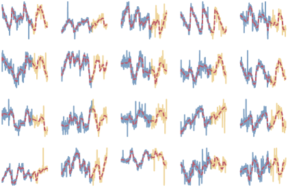
Figure 1: Fitting rPSMF on synthetic data with $t$-distributed noise. Observed time series (blue) with unobserved future data (yellow) and the reconstruction from the model (red).

We evaluate our method in several experiments. In the first two experiments, we show how PSMF can simultaneously learn the dictionary and the parameters of a nonlinear subspace model on synthetic and real data. The third experiment illustrates how our method can be beneficial for change point detection. Finally, our fourth experiment highlights how our method outperforms other MF methods for missing value imputation (modifications to handle missing data in our method are given in Supp. E). Additionally, in Supp. H and Supp. I we present experiments on the convergence of our method and recursive parameter estimation, respectively. Code to reproduce our experiments is available in an online repository.

4.1 A synthetic nonlinear periodic subspace

To demonstrate the ability of the algorithm to learn a dictionary and a structured subspace jointly, we choose $x_{0}=\mu_{0}$ and $P_{0}=0$ and use $x_{k}=f_{\theta}(x_{k-1})=\cos(2\pi\theta k+x_{k-1})$, where $\theta\in{\mathbb{R}}_{+}^{r}$ and $Q_{k}=0$ for all $k\geq 1$. This defines a deterministic subspace with highly periodic structure. We choose $d=20$ and $r=6$ and generate the data from the model with $\theta^{\star}=10^{-3}\cdot[1,2,3,4,5,6]$. We explore both Gaussian and $t$-distributed measurement noise (the latter using 3 degrees of freedom) and both PMSF and rPSMF. We initialize $C_{0}$ randomly and draw $\theta_{0}$ from a uniform distribution on $[0,0.1]^{r}$. We set $V_{0}=v_{0}\otimes I_{r}$ with $v_{0}=0.1$ and use $\lambda_{0}=1.8$ for rPSMF. We furthermore use iterative parameter estimation using the Adam optimizer (Kingma and Ba,, 2015) with standard parameterization, and re-initialize $V_{0}$, $R_{0}$, and $Q_{0}$ at every (outer) iteration (see Supp. G.1 for details). The generated data can be seen in Fig. 1. The task is thus to identify the correct subspace structure by estimating $\theta$ as well as to learn the dictionary matrix $C$.

Fig. 1 shows a run with $t$-distributed noise fitted by rPSMF. We can see that even though the data exhibits clear outliers the model successfully learns both the underlying generative model and its parameters. Expanded results for PSMF are available in Supp. G.1.

4.2 Forecasting real-world data using a nonlinear subspace

To illustrate the advantage of specifying an appropriate subspace model, we explore weather-related features in a dataset on air quality in Beijing (Liang et al.,, 2015), obtained from the UCI repository (Bache and Lichman,, 2013). To simplify the problem the dataset is sampled at every 100 steps, resulting in $n=439$ observations and $d=3$ variables (dew point, temperature, and atmospheric pressure). We compare PSMF using a random walk subspace model, $x_{k}=f(x_{k-1})=x_{k-1}$, against a periodic subspace model $x_{k}=f_{\theta}(x_{k-1})=\theta_{1}\sin(2\pi\theta_{2}k+\theta_{3}x_{k-1})+\theta_{4}\cos(2\pi\theta_{5}k+\theta_{6}x_{k-1})$. In both settings we use $r=1$, run iterative PSMF with 100 iterations, and withhold 20% of the data for prediction. Fig. 2 illustrates the benefit of an appropriate subspace model on forecasting performance and confirms that PSMF can recover nonlinear subspace dynamics in real-world datasets.

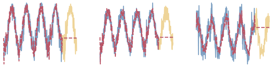
(a) Random walk subspace model.

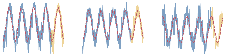
(b) Periodic subspace model.

Figure 2: Comparison of random walk and periodic subspace models on a time series of weather measurements in Beijing. This shows that with the appropriate subspace model, PSMF correctly identifies the nonlinear dynamics of the data and accurately extrapolates into the future. Colors as in Fig. 1.

4.3 Learning representations for robust multivariate changepoint detection

Table 1: Detection accuracy of a changepoint within a window of length $30$ using data and GP features, against the degrees of freedom of the $t$-distributed noise on $\pm 5\%$ of measurements. Averaged over $1000$ different synthetic datasets with $r=10$.

	Degrees of freedom of $t$-contamination
	1.5	1.6	1.7	1.8	1.9
PELT-PSMF	85%	89%	92%	94%	95%
PELT-Data	76%	81%	83%	85%	85%
MBOCPD	54%	58%	61%	69%	72%

Table 2: Imputation error and runtime on several datasets using 30% missing values, averaged over 100 random repetitions. An asterisk marks offline methods.

	Imputation RMSE					Runtime (s)
	NO2	PM10	PM25	S&P500	Gas	NO2	PM10	PM25	S&P500	Gas
PSMF	$\underset{{\scriptscriptstyle(0.13)}}{\textbf{5.72}}$	$\underset{{\scriptscriptstyle(0.31)}}{\textbf{7.44}}$	$\underset{{\scriptscriptstyle(0.23)}}{3.55}$	$\underset{{\scriptscriptstyle\;\;(2.42)}}{11.56}$	$\underset{{\scriptscriptstyle(1.07)}}{\textbf{6.16}}$	2.76	2.61	1.91	9.37	96.75
rPSMF	$\underset{{\scriptscriptstyle(0.22)}}{5.73}$	$\underset{{\scriptscriptstyle(0.45)}}{7.54}$	$\underset{{\scriptscriptstyle(0.21)}}{\textbf{3.50}}$	$\underset{{\scriptscriptstyle\;\;(1.67)}}{\textbf{10.24}}$	$\underset{{\scriptscriptstyle(1.51)}}{6.18}$	2.93	2.03	2.02	13.06	111.89
MLE-SMF	$\underset{{\scriptscriptstyle\;\;(0.58)}}{11.17}$	$\underset{{\scriptscriptstyle(0.31)}}{9.50}$	$\underset{{\scriptscriptstyle(0.36)}}{4.90}$	$\underset{{\scriptscriptstyle\;\;(0.83)}}{30.20}$	$\underset{{\scriptscriptstyle\;\;\;(19.95)}}{111.16}$	2.54	2.38	1.69	9.72	87.22
TMF	$\underset{{\scriptscriptstyle(0.14)}}{7.73}$	$\underset{{\scriptscriptstyle(0.22)}}{8.08}$	$\underset{{\scriptscriptstyle(0.31)}}{4.65}$	$\underset{{\scriptscriptstyle\;\;(0.79)}}{34.90}$	$\underset{{\scriptscriptstyle\;\;(8.64)}}{74.80}$	1.03	0.97	0.65	4.19	34.23
PMF*	$\underset{{\scriptscriptstyle\;\;(0.06)}}{10.51}$	$\underset{{\scriptscriptstyle\;\;(0.18)}}{10.49}$	$\underset{{\scriptscriptstyle(0.18)}}{4.05}$	$\underset{{\scriptscriptstyle\;\;(1.43)}}{40.69}$	$\underset{{\scriptscriptstyle\;\;(0.05)}}{23.77}$	1.96	1.72	0.61	2.79	28.35
BPMF*	$\underset{{\scriptscriptstyle(0.20)}}{9.22}$	$\underset{{\scriptscriptstyle(0.20)}}{8.50}$	$\underset{{\scriptscriptstyle(0.18)}}{3.68}$	$\underset{{\scriptscriptstyle\;\;(0.65)}}{27.64}$	$\underset{{\scriptscriptstyle\;\;(0.28)}}{18.31}$	2.89	2.71	1.61	3.68	91.30

Table 3: Average coverage proportion of the missing data by the $2\sigma$ uncertainty bars of the posterior predictive estimates, averaged over 100 repetitions.

	NO2	PM10	PM25	S&P500	Gas
PSMF	0.76	0.76	0.92	0.83	0.89
rPSMF	0.85	0.89	0.87	0.83	0.86
MLE-SMF	0.43	0.56	0.80	0.48	0.56

We generate time series with $d=20$ dimensions where only $3$ exhibit a structural change. In addition to standard Gaussian noise we contaminate 5% of the entries on average using heavy-tailed $t$-distributed noise with degrees of freedom varying from $1.5$ to $1.9$. To learn the structural changes and be robust against the heavy-tailed noise, we design a smooth subspace model $(x_{i}(t))_{t\geq 0}$ for $i=1,\ldots,r$ in continuous-time using a Gaussian process (GP) prior, $x_{i}(t)\sim\mathcal{GP}(0,\mathsf{k}_{\nu}(t,t^{\prime}))$, with Matérn-${3/2}$ kernel with $\nu=3/2$ (Williams and Rasmussen,, 2006). This particular GP admits a state-space representation amenable to filtering (Hartikainen and Särkkä,, 2010) as it can be recast (Särkkä et al.,, 2013) as the stochastic differential equation (SDE):

$$\frac{\,{\mathrm{d}}\mathsf{x}_{i}(t)}{\,{\mathrm{d}}t}=\begin{bmatrix}0&1\\ -\kappa^{2}&-2\kappa\end{bmatrix}\mathsf{x}_{i}(t)+\begin{bmatrix}0\\ 1\end{bmatrix}w_{i}(t)$$ (29)

where $\mathsf{x}_{i}(t)=[x_{i}(t),\,{\mathrm{d}}x_{i}(t)/\,{\mathrm{d}}t]$ and $\kappa=\sqrt{2\nu}/{\ell}$. We choose $\sigma^{2}=0.1$ and $\ell=0.1$ and discretize equation (29) with the step-size $\gamma=0.001$. We discretize the SDEs for $i=1,\ldots,r$ and construct a joint state which leads to a linear dynamical system in $2r$ dimensions for which we can run PSMF. The details of the discretization and the corresponding PSMF model are given in Supp. G.2, along with an illustration of the learned GP features.

We run PSMF with the discretized GP subspace model with $r=10$. We note that the goal is to obtain a representation that is helpful for changepoint detection. We first employ PELT (Killick et al.,, 2012) as an example changepoint detection method directly on the time-series to create a baseline. Then, we estimate a smooth GP subspace with PSMF and run PELT on that subspace (i.e., the columns of $X$). We additionally compare against a multivariate implementation of Bayesian online CPD (MBOCPD, Adams and MacKay,, 2007). The results in Table 1 clearly show the improved performance and robustness of PSMF.

4.4 Missing Value Imputation

Finally, we test our method on imputation of missing values in time-series data. We consider data from various domains, including three time series of air pollutants measured across London, a gas-sensor dataset by Burgués et al., (2018) obtained from the UCI repository (Bache and Lichman,, 2013), and five years of daily closing prices of stocks in the S&P500 index. The air pollution series contain hourly measurements between 2018-06-01 and 2018-12-01 ($n=4393$) and consist of NO₂ measured at $d=83$ sites, PM10 from $d=74$ sites, and PM25 measured at $d=26$ sites. For the gas sensor dataset (Gas) we have $n=295,719$ and $d=19$ and for the S&P500 dataset we have $n=1259$ and $d=505$. The air pollution datasets contain a high number of missing values due to sensor failures and maintenance, and the stock price dataset contains missing values due to stocks being added to the index.

To test the accuracy of imputations, we randomly remove segments of length $20$ and thereby construct datasets with $30\%$ missing data. We compare our methods against four baselines. The first is an MLE approach to online probabilistic matrix factorization (Yildirim et al.,, 2012; Sun et al.,, 2012; Févotte et al.,, 2013) where we construct an SSM where $C$ is constant, denoted as MLE-SMF. The second is temporal matrix factorization (TMF) which is an adaptation of the optimisation-based method of Yu et al., (2016). We also add two popular offline methods that can only operate on the entire data matrix at once: PMF (Mnih and Salakhutdinov,, 2008) and BPMF (Salakhutdinov and Mnih,, 2008).

We assume the subspace model to be a random walk, $f_{\theta}(x)=x$, thus avoiding the parameter estimation problem, and we use the final estimates of $C$ and $X$ for data imputation. We formulate TMF with the weight matrix set to identity for tractability. We set $r=10$ for all methods and datasets. For PSMF and MLE-SMF we set $R_{k}:=R=\rho\otimes I_{r}$ with $\rho=10$, $P_{0}=I_{r}$, $Q_{k}:=Q=q\otimes I_{r}$ with $q=0.1$. For rPSMF we use $R_{0}=R$ and $Q_{0}=Q$ and set $\lambda_{0}=1.8$. For PSMF and rPSMF we let $V_{0}=v_{0}\otimes I_{r}$ where $v_{0}=2$. All methods are run for two iterations (epochs) over the data to limit run-times, and we repeat the experiments $100$ times with different initializations and missing data patterns. In Table 2 we see that PSMF and rPSMF attain lower RMSEs compared to all other methods and that they are competitive in terms of running time. The advantage of our method is especially noticeable on the $\text{NO}_{2}$, SP500, and Gas datasets.

We can also measure the proportion of missing values that lie within a $2\sigma$ coverage interval of the approximate posterior distribution. Table 3 shows how our method improves over the uncertainty quantification of MLE-SMF (the other methods do not provide a posterior distribution). This illustrates the added value of the matrix-variate prior on $C$, as well as our inference scheme. Note that rPSMF obtains a higher coverage percentage than PSMF on three of the datasets, which is due to the sequential updating of the noise covariances. Additional results with 20% and 40% missing data are available in Supp. G.3.

5 CONCLUSION

We have recast the problem of probabilistic dimensionality reduction for time-series as a joint state filtering and parameter estimation problem in a state-space model. Our model is fully probabilistic and we provide a tractable sequential inference algorithm to run the method with linear computational complexity with respect to the number of data points. Our algorithm is purely recursive and can be used in streaming settings. In particular, the batch algorithms that we compare to (such as PMF and BPMF) would incur the full runtime costs when a new sample arrives. This would likely be prohibitive in practice (e.g. BPMF takes 90 seconds for the Gas dataset) and would increase significantly with the dataset size. By contrast, our method only requires incremental computation to process a new sample (e.g. on the order of milliseconds for the Gas dataset).

We have also extended our initial model into a robust version to handle model misspecification and datasets contaminated with outliers. The robust version of our method has been shown to be advantageous in light of model misspecification.

The state-space formulation of the problem opens many directions for future research such as (i) the use of general models for $f_{\theta}$ or non-Gaussian likelihoods, (ii) the exploration of the use of switching SSMs, and (iii) the integration of more advanced inference techniques such as ensemble Kalman filters or Monte Carlo-based methods for nonlinear and non-Gaussian generalizations of our model.

Acknowledgments

Ö. D. A. is supported by the Lloyd’s Register Foundation Data Centric Engineering Programme and EPSRC Programme Grant EP/R034710/1. The work of GvdB is supported in part by EPSRC grant EP/N510129/1 to the Alan Turing Institute. T. D. acknowledges support from EPSRC EP/T004134/1, UKRI Turing AI Fellowship EP/V02678X/1, and Lloyd’s Register Foundation programme on Data Centric Engineering through the London Air Quality project.

 

Supplementary Material

 

Appendix A PRELIMINARIES

In this section, we list some linear algebra properties related to Kronecker products, which will be used in proofs.

We denote the Kronecker product $\otimes$. Let $A$ be of dimension ${m\times r}$ and $B$ be of dimension ${r\times n}$; then Harville, (1997),

$${A}\otimes{B}=\begin{bmatrix}a_{11}{B}&\cdots&a_{1r}{B}\\ \vdots&\ddots&\vdots\\ a_{m1}{B}&\cdots&a_{mr}{B}\end{bmatrix}.$$ (A.1)

For matrices $A,B$ and $X$, it holds that

$${\operatorname{vec}}(AXB)=(B^{\top}\otimes A){\operatorname{vec}}(X).$$ (A.2)

We can particularize this formula for an $r\times 1$ vector $x$ as

$$Ax={\operatorname{vec}}(Ax)=(x^{\top}\otimes I_{d}){\operatorname{vec}}(A).$$ (A.3)

Kronecker product has the following mixed product property Harville, (1997)

$$(A\otimes B)(C\otimes D)=(AC)\otimes(BD),$$ (A.4)

and the inversion property Harville, (1997)

$$(A\otimes B)^{-1}=A^{-1}\otimes B^{-1}.$$ (A.5)

Appendix B PROOF OF PROPOSITION 1

We adapt the proof in Akyildiz and Míguez, (2019). We first note that for a Gaussian prior $\tilde{p}(c|y_{1:k-1})={\mathcal{N}}(c;c_{k-1},L_{k-1})$ and likelihood of the form $p(y_{k}|y_{1:k-1},c)={\mathcal{N}}(y_{k};H_{k}c,G_{k})$, we can write the posterior analytically $\tilde{p}(c|y_{1:k})={\mathcal{N}}(c;c_{k},L_{k})$ where (see, e.g., Bishop, (2006))

$$c_{k} =c_{k-1}+L_{k-1}H_{k}^{\top}(H_{k}L_{k-1}H_{k}^{\top}+G_{k})^{-1}(y_{k}-H_{k}c_{k-1}),$$ (B.1)

$$L_{k} =L_{k-1}-L_{k-1}H_{k}^{\top}(H_{k}L_{k-1}H_{k}^{\top}+G_{k})^{-1}H_{k}L_{k-1}.$$ (B.2)

In order to obtain an efficient matrix-variate update rule using this vector-form update, we first rewrite the likelihood as

$$\tilde{p}(y_{k}|c,y_{1:k-1}) ={\mathcal{N}}(y_{k};H_{k}c,G_{k})$$ (B.3)

where $H_{k}=\bar{\mu}_{k}^{\top}\otimes I_{d}$ and $G_{k}=\eta_{k}\otimes I_{d}$. We note that, we have $L_{0}=V_{0}\otimes I_{d}$ and we assume as an induction hypothesis that $L_{k-1}=V_{k-1}\otimes I_{d}$. We start by showing that the update (B.2) can be greatly simplified using the special structure we impose. By the mixed product property (A.4) and the inversion property (A.5) we obtain

$$\left[H_{k}L_{k-1}H_{k}^{\top}+G_{k}\right]^{-1}=\left[(\bar{\mu}_{k}^{\top}\otimes I_{d})(V_{k-1}\otimes I_{d})(\bar{\mu}_{k}\otimes I_{d})+\eta_{k}\otimes I_{d}\right]^{-1}=(\bar{\mu}_{k}^{\top}V_{k-1}\bar{\mu}_{k}+\eta_{k})^{-1}\otimes I_{d}$$ (B.4)

and therefore,

$$L_{k}= \,\,(V_{k-1}\otimes I_{d})-(V_{k-1}\bar{\mu}_{k}\otimes I_{d})\times((\bar{\mu}_{k}^{\top}V_{k-1}\bar{\mu}_{k}+\eta_{k})^{-1}\otimes I_{d})\times(\bar{\mu}_{k}^{\top}V_{k-1}\otimes I_{d}).$$ (B.5)

One more use of the mixed product property (A.4) yields

$$L_{k}=\left(V_{k-1}-\frac{V_{k-1}\bar{\mu}_{k}\bar{\mu}_{k}^{\top}V_{k-1}}{\bar{\mu}_{k}^{\top}V_{k-1}\bar{\mu}_{k}+\eta_{k}}\right)\otimes I_{d}.$$ (B.6)

Thus, we have $L_{k}=V_{k}\otimes I_{d}$ where,

$$V_{k}=V_{k-1}-\frac{V_{k-1}\bar{\mu}_{k}\bar{\mu}_{k}^{\top}V_{k-1}}{\bar{\mu}_{k}^{\top}V_{k-1}\bar{\mu}_{k}+\eta_{k}}.$$ (B.7)

We have shown that the sequence $(L_{k})_{k\geq 1}$ preserves the Kronecker structure. Next, we substitute $L_{k-1}=V_{k-1}\otimes I_{d}$, $H_{k}=\bar{\mu}_{k}^{\top}\otimes I_{d}$ and $G_{k}=\eta_{k}\otimes I_{d}$ into (B.1) and we obtain

$$c_{k}=\,\, c_{k-1}+(V_{k-1}\otimes I_{d})(\bar{\mu}_{k}\otimes I_{d})\times\left((\bar{\mu}_{k}^{\top}V_{k-1}\bar{\mu}_{k}+\eta_{k})^{-1}\otimes I_{d}\right)\times(y_{k}-(\bar{\mu}_{k}^{\top}\otimes I_{d})c_{k-1}).$$ (B.8)

The use of the mixed product property (A.4) leaves us with

$$c_{k}=\,\, c_{k-1}+(V_{k-1}\bar{\mu}_{k}\otimes I_{d})\left((\bar{\mu}_{k}^{\top}V_{k-1}\bar{\mu}_{k}+\eta_{k})\otimes I_{d}\right)^{-1}\times(y_{k}-(\bar{\mu}_{k}^{\top}\otimes I_{d})c_{k-1}).$$ (B.9)

Using (A.5) and again (A.4) yields

$$c_{k}=c_{k-1}+ \left[\frac{V_{k-1}\bar{\mu}_{k}}{\bar{\mu}_{k}^{\top}V_{k-1}\bar{\mu}_{k}+\eta_{k}}\otimes I_{d}\right]\times(y_{k}-(\bar{\mu}_{k}^{\top}\otimes I_{d})c_{k-1}).$$ (B.10)

Using (A.3), we get

$$c_{k}=c_{k-1}+\left[\frac{V_{k-1}\bar{\mu}_{k}}{\bar{\mu}_{k}^{\top}V_{k-1}\bar{\mu}_{k}+\eta_{k}}\otimes I_{d}\right](y_{k}-C_{k-1}\bar{\mu}_{k}).$$ (B.11)

We now note that $(y_{k}-C_{k-1}\bar{\mu}_{k})$ and $\frac{V_{k-1}\bar{\mu}_{k}}{\bar{\mu}_{k}^{\top}V_{k-1}\bar{\mu}_{k}+\eta_{k}}$ are vectors. Hence, rewriting the above expression as

$$c_{k}=c_{k-1} +\left[{\operatorname{vec}}\left(\frac{V_{k-1}\bar{\mu}_{k}}{\bar{\mu}_{k}^{\top}V_{k-1}\bar{\mu}_{k}+\eta_{k}}\right)\otimes I_{d}\right]\times{\operatorname{vec}}(y_{k}-C_{k-1}\bar{\mu}_{k}),$$ (B.12)

we can apply (A.3) and obtain

$$c_{k}=c_{k-1}+{\operatorname{vec}}\left(\frac{(y_{k}-C_{k-1}\bar{\mu}_{k})\bar{\mu}_{k}^{\top}V_{k-1}^{\top}}{\bar{\mu}_{k}^{\top}V_{k-1}\bar{\mu}_{k}+\eta_{k}}\right).$$ (B.13)

Hence up to a reshaping operation, we have the update rule (20) and conclude the proof. ∎

Appendix C PROOF OF PROPOSITION 2

Recall that we have a posterior of the form at time $k-1$

$$p(c|y_{1:k-1})={\mathcal{N}}(c;c_{k-1},V_{k-1}\otimes I_{d}),$$ (C.1)

and we are given the likelihood

$$p(y_{k}|c,x_{k})={\mathcal{N}}(y_{k};(x_{k}\otimes I_{d})c,R_{k}).$$ (C.2)

We are interested in computing

$$p(y_{k}|y_{1:k-1},x_{k}) =\int p(c|y_{1:k-1})p(y_{k}|c,x_{k})\,{\mathrm{d}}c.$$ (C.3)

This integral is analytically tractable since both distributions are Gaussian and it is given by Bishop, (2006)

$$p(y_{k}|y_{1:k-1},x_{k})={\mathcal{N}}(y_{k};(x_{k}^{\top}\otimes I_{d})c_{k},R_{k}+(x_{k}^{\top}\otimes I_{d})(V_{k-1}\otimes I_{d})(x_{k}\otimes I_{d})).$$ (C.4)

Using the mixed product property (A.4), one obtains

$$p(y_{k}|y_{1:k-1},x_{k})={\mathcal{N}}(y_{k};C_{k-1}x_{k},R_{k}+x_{k}^{\top}V_{k-1}x_{k}\otimes I_{d}).$$ (C.5)

Appendix D DERIVATION OF THE NEGATIVE LOG-LIKELIHOOD

We obtain the marginal likelihood as

$$\tilde{p}_{\theta}(y_{k}|y_{1:k-1}) =\int\tilde{p}(y_{k}|y_{1:k-1},c)\tilde{p}(c|y_{1:k-1})\,{\mathrm{d}}c$$ (D.1)

$$={\mathcal{N}}(y_{k};C\bar{\mu}_{k},\eta_{k}\otimes I_{d}){\mathcal{N}}(c;c_{k-1},V_{k-1}\otimes I_{d})$$ (D.2)

$$={\mathcal{N}}(y_{k};(\bar{\mu}_{k}^{\top}\otimes I_{d})c,\eta_{k}\otimes I_{d}){\mathcal{N}}(c;c_{k-1},V_{k-1}\otimes I_{d})$$ (D.3)

$$={\mathcal{N}}(y_{k};(\bar{\mu}_{k}^{\top}\otimes I_{d})c_{k-1},(\bar{\mu}_{k}^{\top}V_{k-1}\bar{\mu}_{k}+\eta_{k})\otimes I_{d})$$ (D.4)

$$={\mathcal{N}}\left(y_{k};C_{k-1}f_{\theta}(\mu_{k-1}),\left(\|f_{\theta}(\mu_{k-1})\|^{2}_{V_{k-1}}+\eta_{k}\right)\otimes I_{d}\right).$$ (D.5)

where in the last line we have used the fact that $\bar{\mu}_{k}=f_{\theta}(\mu_{k-1})$ and properties from Supp. A. It is then straightforward to show that

$$-\log\tilde{p}_{\theta}(y_{k}\,|\,y_{1:k-1})=-\log\left[(2\pi)^{-d/2}\cdot|(\|f_{\theta}(\mu_{k-1})\|^{2}_{V_{k-1}}+\eta_{k})\otimes I_{d}|^{-1/2}\right.$$ (D.6)

$$\quad\left.\cdot\exp\left(-\tfrac{1}{2}(y_{k}-C_{k-1}f_{\theta}(\mu_{k-1}))^{\top}\left(\|f_{\theta}(\mu_{k-1})\|^{2}_{V_{k-1}}+\eta_{k})\otimes I_{d}\right)^{-1}(y_{k}-C_{k-1}f_{\theta}(\mu_{k-1})\right)\right]$$ (D.7)

which simplifies to

$$-\log\tilde{p}_{\theta}(y_{k}\,|\,y_{1:k-1}) =\frac{d}{2}\log(2\pi)+\frac{d}{2}\log(\|f_{\theta}(\mu_{k-1})\|^{2}_{V_{k-1}}+\eta_{k})+\tfrac{1}{2}\frac{\|y_{k}-C_{k-1}f_{\theta}(\mu_{k-1})\|^{2}}{\|f_{\theta}(\mu_{k-1})\|^{2}_{V_{k-1}}+\eta_{k}}.$$ (D.8)

Appendix E THE PROBABILISTIC MODEL TO HANDLE MISSING DATA

To obtain update rules that can explicitly handle missing data, we only need to modify the likelihood. When we receive an observation vector with missing entries, we model it as $z_{k}=m_{k}\odot y_{k}$ where $m_{k}\in\{0,1\}^{d}$ is a mask vector that contains zeros for missing entries and ones otherwise. We note that $z_{k}=M_{k}y_{k}$ where $M_{k}=\operatorname{diag}(m_{k})$, which results in the likelihood $p(z_{k}|c,x_{k})={\mathcal{N}}(z_{k};M_{k}Cx_{k},M_{k}R_{k}M_{k}^{\top})$. The update rules for PSMF and the robust model, rPSMF, can be easily re-derived using this likelihood and are essentially identical to Algorithm 1 with masks. Here we discuss the case of PSMF with missing values, rPSMF with missing values is discussed in Supp. F.

We define the probabilistic model with missing data as

$$p(C) =\mathcal{MN}(C;C_{0},I_{d},V_{0}),$$ (E.1)

$$p(x_{0}) ={\mathcal{N}}(x_{0};\mu_{0},P_{0}),$$ (E.2)

$$p_{\theta}(x_{k}|x_{k-1}) ={\mathcal{N}}(x_{k};f_{\theta}(x_{k-1}),Q_{k}),$$ (E.3)

$$p(z_{k}|x_{k},C) ={\mathcal{N}}(z_{k};M_{k}Cx_{k},M_{k}R_{k}M_{k}^{\top}).$$ (E.4)

This model can explicitly handle the missing data when $(M_{k})_{k\geq 1}$ (the missing data patterns) are given. The update rules for this model are defined using masks and are similar to the full data case. In what follows, we derive the update rules for this model by explicitly handling the masks and placing them into our updates formally. For the missing-data case, however, we need a minor approximation in the covariance update rule in order to keep the method efficient. Assume that we are given $\tilde{p}(c|z_{1:k-1})={\mathcal{N}}(c;c_{k-1},V_{k-1}\otimes I_{d})$ and the likelihood

$$\tilde{p}(z_{k}|c,z_{1:k-1})={\mathcal{N}}(z_{k};M_{k}C\bar{\mu}_{k},\eta_{k}\otimes I_{d})$$ (E.5)

where

$$\eta_{k}=\frac{{\operatorname{Tr}}(M_{k}R_{k}M_{k}^{\top}+M_{k}C_{k-1}\bar{P}_{k}C_{k-1}^{\top}M_{k}^{\top})}{m}.$$ (E.6)

In the sequel, we derive the update rules corresponding to the our method with missing data. The derivation relies on the proof of Prop. 1. We note that using (A.2), we can obtain the likelihood

$$\tilde{p}(z_{k}|c,z_{1:k-1})={\mathcal{N}}(z_{k};H_{k}c,\eta_{k}\otimes I_{d})$$ (E.7)

where $c={\operatorname{vec}}(C)$ and $H_{k}=\bar{\mu}_{k}^{\top}\otimes M_{k}$. Deriving the posterior in the same way as in the proof of Prop. 1, and using the approximation $\bar{\mu}_{k}^{\top}V_{k-1}\bar{\mu}_{k}\otimes M_{k}\approx\bar{\mu}_{k}^{\top}V_{k-1}\bar{\mu}_{k}\otimes I_{d}$, leaves us with the covariance update in the form

$$P_{k}=V_{k-1}\otimes I_{d}-\frac{V_{k-1}\bar{\mu}_{k}\bar{\mu}_{k}^{\top}V_{k-1}}{\bar{\mu}_{k}^{\top}V_{k-1}\bar{\mu}_{k}+\eta_{k}}\otimes M_{k}.$$ (E.8)

Unlike the previous case, this covariance does not simplify to a form $P_{k}=V_{k}\otimes I_{d}$ easily. For this reason, we approximate it as

$$P_{k}\approx V_{k}\otimes I_{d},$$ (E.9)

where $V_{k}$ is in the same form of missing-data free updates. To update the mean, we proceed in a similar way as in the proof of Prop. 1 as well. Straightforward calculations lead to the update

$$C_{k}=C_{k-1}+\frac{(z_{k}-M_{k}C_{k-1}\bar{\mu}_{k})\bar{\mu}_{k}^{\top}V_{k-1}}{\bar{\mu}_{k}^{\top}V_{k-1}\bar{\mu}_{k}+\eta_{k}},\quad\mbox{ for $k\geq 1$.}$$ (E.10)

To update $x_{k}$, once we fix $C_{k-1}$, everything straightforwardly follows by replacing $C_{k-1}$ by $M_{k}C_{k-1}$ in the update rules for $(x_{k})_{k\geq 1}$. Finally, the negative log-likelihood $\tilde{p}_{\theta}(z_{k}|z_{1:k-1})$ can be derived similarly to the non-missing case in Sec. 3.2.5, and equals

$$-\log\tilde{p}_{\theta}(z_{k}|z_{1:k-1})\stackrel{{\scriptstyle c}}{{=}}\tfrac{1}{2}\sum_{j=1}^{d}\log u_{jk}+\tfrac{1}{2}(z_{k}-M_{k}C_{k-1}f_{\theta}(\mu_{k-1}))^{\top}U_{k}^{-1}(z_{k}-M_{k}C_{k-1}f_{\theta}(\mu_{k-1})),$$ (E.11)

where $\stackrel{{\scriptstyle c}}{{=}}$ denotes equality up to constants that do not depend on $\theta$ and $U_{k}=\|f_{\theta}(\mu_{k-1})\|_{V_{k-1}}^{2}\otimes M_{k}+\eta_{k}\otimes I_{d}$ is a $d$-dimensional diagonal matrix with elements $u_{jk}$ for $j=1,\ldots,d$.

Appendix F THE ROBUST MODEL

Recall that the model definitions for robust PSMF are as follows

$$p(s) ={\mathcal{IG}}(s;\lambda_{0}/2,\lambda_{0}/2)$$ (F.1)

$$p(C\,|\,s) =\mathcal{MN}(C;C_{0},I_{d},sV_{0})),$$ (F.2)

$$p(x_{0}\,|\,s) ={\mathcal{N}}(x_{0};\mu_{0},sP_{0}),$$ (F.3)

$$p_{\theta}(x_{k}\,|\,x_{k-1},s) ={\mathcal{N}}(x_{k};f_{\theta}(x_{k-1}),sQ_{0}),$$ (F.4)

$$p(y_{k}\,|\,x_{k},C,s) ={\mathcal{N}}(y_{k};Cx_{k},sR_{0}),$$ (F.5)

Before we present the derivation, we recall the following definitions.

Definition 1 (Inverse-Gamma Distribution).

The inverse-gamma distribution is given by

$${\mathcal{IG}}(s;\alpha,\beta)=\frac{\beta^{\alpha}}{\Gamma(\alpha)}\left(\frac{1}{s}\right)^{\alpha+1}\exp\left(-\beta/s\right)$$ (F.6)

for $\alpha,\beta>0$, and with $\Gamma(\cdot)$ the Gamma function.

Definition 2 (Multivariate $t$ Distribution).

For $y\in\mathbb{R}^{d}$ the multivariate $t$ distribution with $\lambda$ degrees of freedom is

$${\mathcal{T}}(y;\mu,\Sigma,\lambda)=\frac{1}{(\pi\lambda)^{d/2}|\Sigma|^{1/2}}\frac{\Gamma((\lambda+d)/2)}{\Gamma(\lambda/2)}\left(1+\frac{\Delta^{2}}{\lambda}\right)^{-(\lambda+d)/2}$$ (F.7)

where $\Delta^{2}=(y-\mu)^{\top}\Sigma^{-1}(y-\mu)$.

Since we again assume the model to be Markovian, we extend the conditional independence and Markov properties (see, e.g., Särkkä,, 2013) to the case with a scale variable

Property 1 (Conditional independence).

The measurement $y_{k}$ given the coefficient $x_{k}$ and scale variable $s$, is conditionally independent of past measurements and coefficients

$$p(y_{k}\,|\,x_{1:k},y_{1:k-1},s)=p(y_{k}\,|\,x_{k},s).$$ (F.8)

Property 2 (Markov property of coefficients).

When conditioning on $s$ the coefficients $x_{k}$ form a Markov sequence, such that

$$p(x_{k}\,|\,x_{1:k-1},y_{1:k-1},s)=p(x_{k}\,|\,x_{k-1},s).$$ (F.9)

We also present the following lemma’s used in the derivation.

Lemma 1.

For $y\in\mathbb{R}^{d}$ with $p(y\,|\,s)={\mathcal{N}}(y;\mu,\Sigma)$ and $p(s)={\mathcal{IG}}(s;\alpha,\beta)$ we have

$$p(y) =\frac{1}{(2\pi\beta)^{d/2}|\Sigma|^{1/2}}\frac{\Gamma(\alpha+d/2)}{\Gamma(\alpha)}\left(1+\frac{\Delta^{2}}{2\beta}\right)^{-(\alpha+d/2)}$$ (F.10)

$$p(s|y) ={\mathcal{IG}}(s;\alpha+d/2,\beta+\tfrac{1}{2}\Delta^{2}).$$ (F.11)

In particular, if $\alpha=\beta=\lambda/2$ then $p(y)={\mathcal{T}}(y;\mu,\Sigma,\lambda)$.

Lemma 2.

If $p(s)={\mathcal{IG}}(s;\alpha,\beta)$ and $\omega=\beta/\alpha$, then $\omega\cdot p(\omega s)={\mathcal{IG}}(s;\alpha,\alpha)$.

Proof.

$$\frac{\beta}{\alpha}p\left(\frac{\beta}{\alpha}s\right)=\frac{\beta}{\alpha}\frac{\beta^{\alpha}}{\Gamma(\alpha)}\left(\frac{\alpha}{\beta s}\right)^{\alpha+1}\exp\left(-\frac{\beta\alpha}{\beta s}\right)=\frac{\alpha^{\alpha}}{\Gamma(\alpha)}\left(\frac{1}{s}\right)^{\alpha+1}\exp\left(-\frac{\alpha}{s}\right)={\mathcal{IG}}(s;\alpha,\alpha).$$ (F.12)

∎

Lemma 3.

For a partitioned random variable $y=[y_{a},y_{b}]^{\top}$ with $y_{a}\in\mathbb{R}^{d_{a}}$ and $y_{b}\in\mathbb{R}^{d_{b}}$ that follows a multivariate $t$ distribution given by

$$p(y)=p(y_{a},y_{b})={\mathcal{T}}\left(\begin{bmatrix}y_{a}\\ y_{b}\end{bmatrix};\begin{bmatrix}\mu_{a}\\ \mu_{b}\end{bmatrix},\begin{bmatrix}\Sigma_{aa}&\Sigma_{ab}\\ \Sigma_{ab}^{\top}&\Sigma_{bb}\end{bmatrix},\lambda\right),$$ (F.13)

the marginal and conditional densities are given by

$$p(y_{b}) ={\mathcal{T}}(y_{b};\mu_{b},\Sigma_{bb},\lambda)$$ (F.14)

$$p(y_{a}\,|\,y_{b}) ={\mathcal{T}}(y_{a};\mu_{a|b},\Sigma_{a|b},\lambda_{a|b}),$$ (F.15)

with

$$\lambda_{a|b} =\lambda+d_{b}$$ (F.16)

$$\mu_{a|b} =\mu_{a}+\Sigma_{ab}\Sigma_{bb}^{-1}(y_{b}-\mu_{b})$$ (F.17)

$$\Sigma_{a|b} =\frac{\lambda+(y_{b}-\mu_{b})^{\top}\Sigma_{bb}^{-1}(y_{b}-\mu_{b})}{\lambda+d_{b}}\left(\Sigma_{aa}-\Sigma_{ab}\Sigma_{bb}^{-1}\Sigma_{ab}^{\top}\right).$$ (F.18)

Proof.

See Roth, (2012) for a derivation. ∎

To derive inference in the robust model, we start from $k=1$ and show how we perform filtering for an entire iteration. While this makes the description longer, we believe it to be more informative for the reader. We begin with prediction of $x_{1}$ given no history ($y_{1:0}=\emptyset$). The predictive distribution of $x_{1}$ is then

$$\tilde{p}(x_{1}\,|\,y_{1:0},s) =\int p(x_{1}\,|\,x_{0},s)p(x_{0}\,|\,y_{1:0},s)\,{\mathrm{d}}x_{0}$$ (F.19)

$$\tilde{p}(x_{1}\,|\,s) =\int p(x_{1}\,|\,x_{0},s)p(x_{0}\,|\,s)\,{\mathrm{d}}x_{0}$$ (F.20)

$$=\int{\mathcal{N}}(x_{1};f_{\theta}(x_{0}),sQ_{0}){\mathcal{N}}(x_{0};\mu_{0},sP_{0})\,{\mathrm{d}}x_{0}$$ (F.21)

$$={\mathcal{N}}(x_{1};f_{\theta}(\mu_{0}),s(Q_{0}+F_{1}P_{0}F_{1}^{\top})),$$ (F.22)

where $F_{1}$ is defined as in the main text. Writing $\bar{\mu}_{1}=f_{\theta}(\mu_{0})$ and $\bar{P}_{1}=Q_{0}+F_{1}P_{0}F_{1}^{\top}$ we get $\tilde{p}(x_{1}\,|\,s)={\mathcal{N}}(x_{1};\bar{\mu}_{1},s\bar{P}_{1})$. Next, we move to the dictionary update. We first have

$$\tilde{p}(y_{1}\,|\,c,y_{1:0},s) =\int p(y_{1}\,|\,c,x_{1},s)p(x_{1}\,|\,y_{1:0},s)\,{\mathrm{d}}x_{1}$$ (F.23)

$$\tilde{p}(y_{1}\,|\,c,s) =\int p(y_{1}\,|\,c,x_{1},s)p(x_{1}\,|\,s)\,{\mathrm{d}}x_{1}$$ (F.24)

$$=\int{\mathcal{N}}(y_{1};Cx_{1},sR_{0}){\mathcal{N}}(x_{1};\bar{\mu}_{1},s\bar{P}_{1})\,{\mathrm{d}}x_{1}$$ (F.25)

$$={\mathcal{N}}(y_{1};C\bar{\mu}_{1},s(R_{0}+C\bar{P}_{1}C^{\top})).$$ (F.26)

As in PSMF, we use the approximation $C\bar{P}_{1}C^{\top}\approx\eta_{1}\otimes I_{d}$ where $\eta_{1}={\operatorname{Tr}}(R_{0}+C_{0}\bar{P}_{1}C_{0}^{\top})/d$. We write this as $\tilde{p}(y_{1}\,|\,c,s)={\mathcal{N}}(y_{1};H_{1}c,sG_{1})$ with $H_{1}=\bar{\mu}_{1}^{\top}\otimes I_{d}$ and $G_{1}=\eta_{1}\otimes I_{d}$. We again assume $\tilde{p}(c\,|\,y_{1:0},s)={\mathcal{N}}(c;c_{0},sL_{0})$ using $L_{0}=V_{0}\otimes I_{d}$, such that

$$\tilde{p}(c,y_{1}\,|\,y_{1:0},s) =\tilde{p}(y_{1}\,|\,c,y_{1:0},s)\tilde{p}(c\,|\,y_{1:0},s)$$ (F.27)

$$\tilde{p}(c,y_{1}\,|\,s) =\tilde{p}(y_{1}\,|\,c,s)\tilde{p}(c\,|\,s)$$ (F.28)

$$={\mathcal{N}}(y_{1};H_{1}c,sG_{1}){\mathcal{N}}(c;c_{0},sL_{0})$$ (F.29)

$$={\mathcal{N}}\left(\begin{bmatrix}c\\ y_{1}\end{bmatrix};\begin{bmatrix}c_{0}\\ H_{1}c_{0}\end{bmatrix},s\begin{bmatrix}L_{0}&L_{0}H_{1}^{\top}\\ H_{1}L_{0}&H_{1}L_{0}H_{1}^{\top}+G_{1}\end{bmatrix}\right)$$ (F.30)

Integrating out $s$ in this expression gives

$$\tilde{p}(c,y_{1})={\mathcal{T}}\left(\begin{bmatrix}c\\ y_{1}\end{bmatrix};\begin{bmatrix}c_{0}\\ H_{1}c_{0}\end{bmatrix},\begin{bmatrix}L_{0}&L_{0}H_{1}^{\top}\\ H_{1}L_{0}&H_{1}L_{0}H_{1}^{\top}+G_{1}\end{bmatrix},\lambda_{0}\right)$$ (F.31)

Conditioning on $y_{1}$ and using Lemma 3 yields $\tilde{p}(c\,|\,y_{1})={\mathcal{T}}(c;c_{1},L_{1},\lambda_{0}+d)$ with

$$c_{1} =c_{0}+L_{0}H_{1}^{\top}\left[H_{1}L_{0}H_{1}^{\top}+G_{1}\right]^{-1}(y_{1}-H_{1}c_{0})$$ (F.32)

$$L_{1} =\phi_{1}\left(L_{0}H_{1}^{\top}\left[H_{1}L_{0}H_{1}^{\top}+G_{1}\right]^{-1}H_{1}L_{0}\right)$$ (F.33)

$$\varphi_{1} =\frac{\lambda_{0}+(y_{1}-H_{1}c_{0})^{\top}\left[H_{1}L_{0}H_{1}^{\top}+G_{1}\right]^{-1}(y_{1}-H_{1}c_{0})}{\lambda_{0}+d}.$$ (F.34)

This is the robust PSMF dictionary update. We see that the mean is updated as in PSMF by comparing to (B.1), and that the covariance update has an additional multiplicative factor $\varphi_{1}$. These expressions can be simplified by plugging in the definitions of $L_{0}$, $H_{1}$, and $G_{1}$, as in Supp. B. Observe that $\tilde{p}(c\,|\,y_{1})$ can no longer be written as an infinite scale mixture with scale variable $s$, as they now differ in degrees of freedom. We will revisit this point below.

For the coefficient update we proceed analogously. First, note that

$$\tilde{p}(y_{1}\,|\,x_{0:1},s) =\int p(y_{1}\,|\,c,x_{0:1},s)p(c\,|\,y_{1:0},s)\,{\mathrm{d}}c$$ (F.35)

$$\tilde{p}(y_{1}\,|\,x_{1},s) =\int p(y_{1}\,|\,c,x_{1},s)p(c\,|\,s)\,{\mathrm{d}}c$$ (F.36)

$$=\int{\mathcal{N}}(y_{1};(x_{1}^{\top}\otimes I_{d})c,sR_{0}){\mathcal{N}}(c;c_{0},sL_{0})\,{\mathrm{d}}c$$ (F.37)

$$={\mathcal{N}}(y_{1};(x_{1}^{\top}\otimes I_{d})c_{0},s(R_{0}+x_{1}^{\top}V_{0}x_{1}\otimes I_{d}))$$ (F.38)

As in the main text, we use the approximation $x_{1}^{\top}V_{0}x_{1}\approx\bar{\mu}_{1}^{\top}V_{0}\bar{\mu}_{1}$ and introduce

$$\bar{R}_{0}=R_{0}+\bar{\mu}_{1}^{\top}V_{0}\bar{\mu}_{1},$$ (F.39)

such that $\tilde{p}(y_{1}\,|\,x_{1},s)={\mathcal{N}}(y_{1};C_{0}x_{1},s\bar{R}_{0})$. We then find the joint distribution between $x_{1}$ and $y_{1}$ as follows

$$\tilde{p}(x_{1},y_{1}\,|\,y_{1:0},s) =\tilde{p}(y_{1}\,|\,y_{1:0},x_{1},s)\tilde{p}(x_{1}\,|\,y_{1:0},s)$$ (F.40)

$$\tilde{p}(x_{1},y_{1}\,|\,s) =\tilde{p}(y_{1}\,|\,x_{1},s)\tilde{p}(x_{1}\,|\,s)$$ (F.41)

$$={\mathcal{N}}(y_{1};C_{0}x_{1},s\bar{R}_{0}){\mathcal{N}}(x_{1};\bar{\mu}_{1},s\bar{P}_{1})$$ (F.42)

$$={\mathcal{N}}\left(\begin{bmatrix}x_{1}\\ y_{1}\end{bmatrix};\begin{bmatrix}\bar{\mu}_{1}\\ C_{0}\bar{\mu}_{1}\end{bmatrix},s\begin{bmatrix}\bar{P}_{1}&\bar{P}_{1}C_{0}^{\top}\\ C_{0}\bar{P}_{1}&C_{0}\bar{P}_{1}C_{0}^{\top}+\bar{R}_{0}\end{bmatrix}\right).$$ (F.43)

Integrating out $s$ in this expression gives

$$\tilde{p}(x_{1},y_{1})={\mathcal{T}}\left(\begin{bmatrix}x_{1}\\ y_{1}\end{bmatrix};\begin{bmatrix}\bar{\mu}_{1}\\ C_{0}\bar{\mu}_{1}\end{bmatrix},\begin{bmatrix}\bar{P}_{1}&\bar{P}_{1}C_{0}^{\top}\\ C_{0}\bar{P}_{1}&C_{0}\bar{P}_{1}C_{0}^{\top}+\bar{R}_{0}\end{bmatrix},\lambda_{0}\right).$$ (F.44)

Conditioning on $y_{1}$ and using Lemma 3 gives $p(x_{1}\,|\,y_{1})={\mathcal{T}}(x_{1};\mu_{1},P_{1},\lambda_{0}+d)$ with

$$\mu_{1} =\bar{\mu}_{1}+\bar{P}_{1}C_{0}^{\top}\left[C_{0}\bar{P}_{1}C_{0}^{\top}+\bar{R}_{0}\right]^{-1}(y_{1}-C_{0}\bar{\mu}_{1})$$ (F.45)

$$P_{1} =\omega_{1}\left(\bar{P}_{1}-\bar{P}_{1}C_{0}^{\top}\left[C_{0}\bar{P}_{1}C_{0}^{\top}+\bar{R}_{0}\right]^{-1}C_{0}\bar{P}_{1}\right)$$ (F.46)

$$\omega_{1} =\frac{\lambda_{0}+(y_{1}-C_{0}\bar{\mu}_{1})^{\top}\left[C_{0}\bar{P}_{1}C_{0}^{\top}+\bar{R}_{0}\right]^{-1}(y_{1}-C_{0}\bar{\mu}_{1})}{\lambda_{0}+d}.$$ (F.47)

This is the robust PSMF coefficient update. Again we see that the mean update for $\mu_{1}$ is the same as in vanilla PSMF, while the covariance update has an additional multiplicative factor $\omega_{1}$. By introducing $\Delta_{1}^{2}=(y_{1}-C_{0}\bar{\mu}_{1})^{\top}\left[C_{0}\bar{P}_{1}C_{0}^{\top}+\bar{R}_{0}\right]^{-1}(y_{1}-C_{0}\bar{\mu}_{1})$ we can simplify this factor to $\omega_{1}=(\lambda_{0}+\Delta_{1}^{2})/(\lambda_{0}+d)$.

Finally, we can compute the posterior of the scale variable, $s$, using Bayes’ theorem,

$$\tilde{p}(s\,|\,y_{1})=\frac{\tilde{p}(y_{1}\,|\,s)p(s)}{\tilde{p}(y_{1})}.$$ (F.48)

We can obtain $\tilde{p}(y_{1}\,|\,s)$ from (F.43), which yields

$$\tilde{p}(y_{1}\,|\,s)={\mathcal{N}}(y_{1};C_{0}\bar{\mu}_{1},s(C_{0}\bar{P}_{1}C_{0}^{\top}+\bar{R}_{0})).$$ (F.49)

Integrating out $s$ gives $\tilde{p}(y_{1})={\mathcal{T}}(y_{1};C_{0}\bar{\mu}_{1},C_{0}\bar{P}_{1}C_{0}^{\top}+\bar{R}_{0},\lambda_{0})$. Thus, by Lemma 1 we have

$$\tilde{p}(s\,|\,y_{1})={\mathcal{IG}}(s;(\lambda_{0}+d)/2,(\lambda_{0}+\Delta_{1}^{2})/2).$$ (F.50)

Having now observed $y_{1}$, we proceed with the next iteration. Note that from the coefficient update we have obtained $p(x_{1}\,|\,y_{1})={\mathcal{T}}(x_{1};\mu_{1},P_{1},\lambda_{0}+d)$. We can write this as a infinite scale mixture by defining $u\sim{\mathcal{IG}}(u;(\lambda_{0}+d)/2,(\lambda_{0}+d)/2)$ and introducing $p(x_{1}\,|\,y_{1},u)={\mathcal{N}}(x_{1};\mu_{1},uP_{1})$. The model definitions give the coefficient dynamics in terms of $s$, as $p(x_{2}\,|\,x_{1},s)={\mathcal{N}}(x_{2};f_{\theta}(x_{1}),sQ_{0})$. This can be written in terms of $u$ by a simple change of variables $u=\omega_{1}^{-1}s$ and using Lemma 2 and (F.50), since

$$\tilde{p}(x_{2}\,|\,x_{1},y_{1}) =\int p(x_{2}\,|\,x_{1},s)p(s\,|\,y_{1})\,{\mathrm{d}}s$$ (F.51)

$$=\int{\mathcal{N}}(x_{2};f_{\theta}(x_{1}),sQ_{0}){\mathcal{IG}}(s;(\lambda_{0}+d)/2,(\lambda_{0}+\Delta_{1}^{2})/2)\,{\mathrm{d}}s$$ (F.52)

$$=\int{\mathcal{N}}(x_{2};f_{\theta}(x_{1}),u\cdot\omega_{1}Q_{0}){\mathcal{IG}}(u;(\lambda_{0}+d)/2,(\lambda_{0}+d)/2)\,{\mathrm{d}}u$$ (F.53)

where we find $p(x_{2}\,|\,x_{1},u)={\mathcal{N}}(x_{2};f_{\theta}(x_{1}),u\cdot\omega_{1}Q_{0})$. We then have that

$$\tilde{p}(x_{2}\,|\,y_{1},u) =\int\tilde{p}(x_{2}\,|\,x_{1},u)\tilde{p}(x_{1}\,|\,y_{1},u)\,{\mathrm{d}}x_{1}$$ (F.54)

$$=\int{\mathcal{N}}(x_{2};f_{\theta}(x_{1}),u\cdot\omega_{1}Q_{0}){\mathcal{N}}(x_{1};\mu_{1},uP_{1})\,{\mathrm{d}}x_{1},$$ (F.55)

which we recognize to be analogous to (F.21). This expression also reveals how the noise covariance $Q_{0}$ is updated, as we may simply define $Q_{1}=\omega_{1}Q_{0}$. This gives $\tilde{p}(x_{2}\,|\,y_{1},u)={\mathcal{N}}(x_{2};\bar{\mu}_{2},u\bar{P}_{2})$ with $\bar{\mu}_{2}$ and $\bar{P}_{2}$ analogous to $\bar{\mu}_{1}$ and $\bar{P}_{1}$ above.

Similar reasoning can be applied to obtain the predictive distribution of $y_{2}$. From the dictionary update we have obtained $\tilde{p}(c\,|\,y_{1})={\mathcal{T}}(c;c_{1},L_{1},\lambda_{0}+d)$, which we can also write as a scale mixture with $u$ as $\tilde{p}(c\,|\,y_{1},u)={\mathcal{N}}(c;c_{1},uL_{1})$. The model definition gives $p(y_{2}\,|\,x_{2},C,s)={\mathcal{N}}(y_{2};Cx_{2},sR_{0})$. Again writing this in terms of $u$ by using the change of variables $u=\omega_{1}^{-1}s$ and Lemma 2 and (F.50), yields $p(y_{2}\,|\,x_{2},C,u)={\mathcal{N}}(y_{2};Cx_{2},u\cdot\omega_{1}R_{0})$. Combining these expressions gives

$$\tilde{p}(y_{2}\,|\,c,y_{1},u)=\int\tilde{p}(y_{2}\,|\,x_{2},C,u)\tilde{p}(c\,|\,y_{1},u)\,{\mathrm{d}}c=\int{\mathcal{N}}(y_{2};(x_{2}^{\top}\otimes I_{d})c,u\cdot\omega_{1}R_{0}){\mathcal{N}}(c;c_{1},uL_{1})\,{\mathrm{d}}c,$$ (F.56)

which is analogous to (F.37). We also see that we can define $R_{1}=\omega_{1}R_{0}$ to update the measurement noise covariance.

We observe in the above derivation that after completing an entire iteration we have obtained a new scale variable $u\sim{\mathcal{IG}}(u;(\lambda_{0}+d)/2,(\lambda_{0}+d)/2)$, and that we have found update rules for the noise covariances $Q$ and $R$. This procedure is repeated at every step, and we can define appropriate notation for this process by setting $s_{0}=s$ and $s_{1}=u$, and generally have scale variables $s_{k}\sim{\mathcal{IG}}(s_{k};\lambda_{k}/2,\lambda_{k}/2)$ with $\lambda_{k}=\lambda_{k-1}+d$. Thus, $s_{k}=\omega_{k}^{-1}s_{k-1}$ with $\omega_{k}=(\lambda_{k-1}+\Delta_{k}^{2})/(\lambda_{k-1}+d)$, which corresponds to Tronarp et al., (2019). The noise covariances are clearly updated as $Q_{k}=\omega_{k}Q_{k-1}$ and $R_{k}=\omega_{k}R_{k-1}$. Algorithm 2 summarizes the steps of robust PSMF, including steps for parameter estimation using both the iterative and recursive approaches.

1:Initialize $\gamma$, $\theta_{0}$, $C_{0}$, $V_{0}$, $\mu_{0}$, $P_{0}$, $Q_{0}$, $R_{0}$.

2:for $i\geq 1$ do

3:     $C_{0}=C_{T}$, $\mu_{0}=\mu_{T}$, $P_{0}=P_{T}$, $V_{0}=V_{T}$.

4:     for $1\leq k\leq T$ do

5:         Predictive mean of $x_{k}$: $\bar{\mu}_{k}=f_{\theta_{i-1}}(\mu_{k-1})$ or $\bar{\mu}_{k}=f_{\theta_{k-1}}(\mu_{k-1})$

6:         Predictive covariance of $x_{k}$

$$\bar{P}_{k}=F_{k}P_{k-1}F_{k}^{\top}+Q_{k-1},\quad\mathrm{where}\quad F_{k}=\frac{\partial f(x)}{\partial x}\Big{|}_{x=\bar{\mu}_{k-1}}$$

7:         Compute scaling factor for the dictionary update

$$\varphi_{k}=\frac{\lambda_{k-1}}{\lambda_{k-1}+d}+\frac{(y_{k}-C_{k-1}\bar{\mu}_{k})^{\top}(y_{k}-C_{k-1}\bar{\mu}_{k})}{(\lambda_{k-1}+d)(\bar{\mu}_{k}^{\top}V_{k-1}\bar{\mu}_{k}+\eta_{k})}$$

          where $\eta_{k}={\operatorname{Tr}}(C_{k-1}\bar{P}_{k}C_{k-1}^{\top}+R_{k-1})/d$.

8:         Mean and covariance updates of the dictionary

$$C_{k}=C_{k-1}+\frac{(y_{k}-C_{k-1}\bar{\mu}_{k})\bar{\mu}_{k}^{\top}V_{k-1}^{\top}}{\bar{\mu}_{k}^{\top}V_{k-1}\bar{\mu}_{k}+\eta_{k}}\quad\text{and}\quad V_{k}=\varphi_{k}\left(V_{k-1}-\frac{V_{k-1}\bar{\mu}_{k}\bar{\mu}_{k}^{\top}V_{k-1}}{\bar{\mu}_{k}^{\top}V_{k-1}\bar{\mu}_{k}+\eta_{k}}\right)$$

9:         Compute scaling factor for the coefficient update

$$\omega_{k}=\frac{\lambda_{k-1}+(y_{k}-C_{k-1}\bar{\mu}_{k})^{\top}S_{k}^{-1}(y_{k}-C_{k-1}\bar{\mu}_{k})}{\lambda_{k-1}+d}$$

          where $S_{k}=C_{k-1}\bar{P}_{k}C_{k-1}^{\top}+\bar{R}_{k-1}$ and $\bar{R}_{k-1}=R_{k-1}+\bar{\mu}_{k}^{\top}V_{k-1}\bar{\mu}_{k}\otimes I_{d}$.

10:         Mean and covariance updates of coefficients

$$\mu_{k}=\bar{\mu}_{k}+\bar{P}_{k}C_{k-1}^{\top}S_{k}^{-1}(y_{k}-C_{k-1}\bar{\mu}_{k})\quad\text{and}\quad P_{k}=\omega_{k}(\bar{P}_{k}-\bar{P}_{k}C_{k-1}^{\top}S_{k}^{-1}C_{k-1}\bar{P}_{k})$$

11:         Update noise covariances: $Q_{k}=\omega_{k}Q_{k-1}$ and $R_{k}=\omega_{k}R_{k-1}$

12:         Update degrees of freedom: $\lambda_{k}=\lambda_{k-1}+d$.

13:         Parameter update: $\theta_{k}=\theta_{k-1}+\gamma\nabla\log\tilde{p}_{\theta}(y_{k}|y_{1:k-1})\big{|}_{\theta=\theta_{k-1}}$ $\triangleright$ recursive version      

14:     Parameter update: $\theta_{i}=\theta_{i-1}+\gamma\sum_{k=1}^{T}\nabla\log\tilde{p}_{\theta}(y_{k}|y_{1:k-1})\big{|}_{\theta=\theta_{i-1}}.$ $\triangleright$ iterative version

Algorithm 2 Iterative and recursive rPSMF

For completeness, we give the approximate negative marginal likelihood $\tilde{p}_{\theta}(y_{k}\,|\,y_{1:k-1})$, similar to Sec. 3.2.5. It follows that

$$\tilde{p}_{\theta}(y_{k}\,|\,y_{1:k-1}) =\iint\tilde{p}(y_{k}\,|\,y_{1:k-1},c,s_{k-1})\tilde{p}(c\,|\,y_{1:k-1},s_{k-1})\,{\mathrm{d}}c\,{\mathrm{d}}s_{k-1}$$ (F.57)

$$=\iint{\mathcal{N}}(y_{k};H_{k}c,s_{k-1}G_{k}){\mathcal{N}}(c;c_{k-1},s_{k-1}L_{k-1})\,{\mathrm{d}}c\,{\mathrm{d}}s_{k-1}$$ (F.58)

$$=\int{\mathcal{N}}(y_{k};H_{k}c_{k-1},s_{k-1}(H_{k}L_{k-1}H_{k}^{\top}+G_{k}))\,{\mathrm{d}}s_{k-1}$$ (F.59)

$$={\mathcal{T}}(y_{k};H_{k}c_{k-1},H_{k}L_{k-1}H_{k}^{\top}+G_{k},\lambda_{k-1})$$ (F.60)

With $H_{k}c_{k-1}=C_{k-1}\bar{\mu}_{k}$ and $H_{k}L_{k-1}H_{k}^{\top}+G_{k}=(\bar{\mu}_{k}^{\top}V_{k-1}\bar{\mu}_{k}+\eta_{k})\otimes I_{d}$ where $\bar{\mu}_{k}=f_{\theta}(\mu_{k-1})$, we find after a brief algebraic exercise that

$$-\log\tilde{p}_{\theta}(y_{k}\,|\,y_{1:k-1}) \stackrel{{\scriptstyle c}}{{=}}\frac{d}{2}\log\left(\|f_{\theta}(\mu_{k-1})\|^{2}_{V_{k-1}}+\eta_{k}\right)$$ (F.61)

$$\qquad\qquad+\left(\frac{\lambda_{k-1}+d}{2}\right)\log\left(1+\frac{\|y_{k}-C_{k-1}f_{\theta}(\mu_{k-1})\|^{2}}{\lambda_{k-1}\left(\|f_{\theta}(\mu_{k-1})\|^{2}_{V_{k-1}}+\eta_{k}\right)}\right)$$ (F.62)

where $\stackrel{{\scriptstyle c}}{{=}}$ again denotes equality up to terms independent of $\theta$. Finally, we note that handling missing values in rPSMF is straightforward and follows the same reasoning as for PSMF in Supp. E.

Appendix G ADDITIONAL DETAILS FOR THE EXPERIMENTS

G.1 Experiment 1

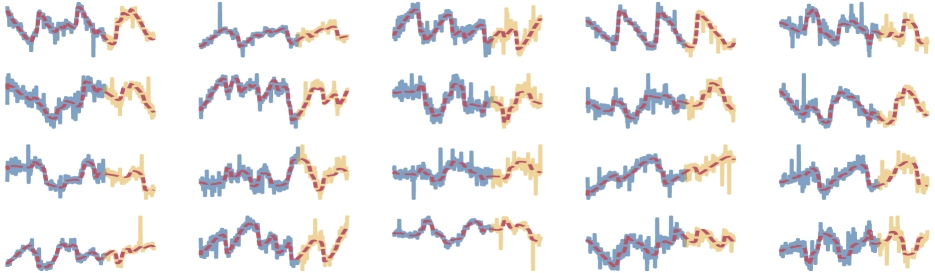
(a) Observed time series (blue) with unobserved future data (yellow) and the reconstruction (red).

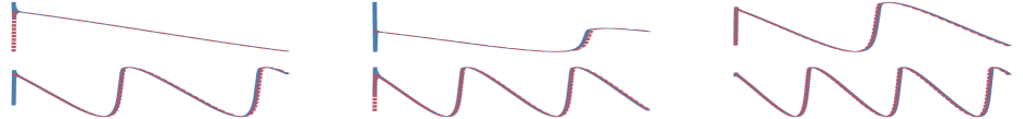
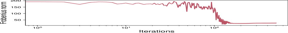
(b) True (blue) and predicted (red) subspace.

(c) Reconstruction error $\|Y-CX\|_{F}^{2}$.

Figure 1: Fitting rPSMF on synthetic data with $t$-distributed noise. Figure (a) illustrates the fit to the observed and unobserved measurements. Figure (b) contains the true and reconstructed subspace, and (c) shows the reconstruction error over outer iterations of the iterative algorithm.

Optimization In this experiment, we have used the Adam optimizer Kingma and Ba, (2015). In particular, instead of implementing the gradient step (26), we replace it with the Adam optimizer. In order to do so, we define the gradient as $g_{i}=\nabla\log\tilde{p}_{\theta}(y_{1:n})\Big{|}_{\theta=\theta_{i-1}}$. Upon computing the gradient $g_{i}$, we first compute the running averages

$$m_{i} =\beta_{1}m_{i-1}+(1-\beta_{1})g_{i}$$ (G.1)

$$v_{i} =\beta_{2}v_{i-1}+(1-\beta_{2})(g_{i}\odot g_{i}),$$ (G.2)

which is then corrected as

$$\hat{m}_{i} =\frac{m_{i}}{1-\beta_{1}^{i}}$$ (G.3)

$$\hat{v}_{i} =\frac{v_{i}}{1-\beta_{2}^{i}}.$$ (G.4)

Finally the parameter update is computed as

$$\theta_{i}=\mathsf{Proj}_{\Theta}\left(\theta_{i-1}+\gamma\frac{\hat{m}_{i}}{\sqrt{\hat{v}_{i}}+\epsilon}\right),$$ (G.5)

where $\mathsf{Proj}$ denotes the projection operator which constrains the parameter to stay positive in each dimension where $\Theta={\mathbb{R}}_{+}\times\cdots\times{\mathbb{R}}_{+}\subset{\mathbb{R}}^{6}$ which is implemented by simple $\max$ operators. We choose the standard parameterization with $\gamma=10^{-3},\beta_{1}=0.9,\beta_{2}=0.999$ and $\epsilon=10^{-8}$.

In these experiments we use an observed time series of length 500 and a series of unobserved future data of length 250. Fig. 1 corresponds to the figure in the main text, but additionally shows how the underlying subspace is recovered and how the Frobenius norm between the reconstructed data and the true data decreases with the number of iterations. Fig. 2 shows a similar result for the PSMF method on normally-distributed data.

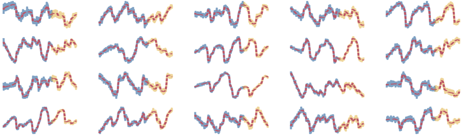
(a) Observed time series (blue) with unobserved future data (yellow) and the reconstruction (red).

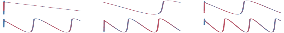
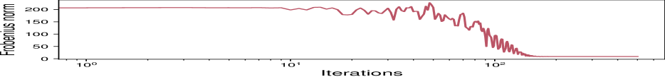
(b) True (blue) and predicted (red) subspace.

(c) Reconstruction error $\|Y-CX\|_{F}^{2}$.

Figure 2: Fitting PSMF on synthetic data with normally distributed noise. Figure (a) illustrates the fit to the observed and unobserved measurements. Figure (b) contains the true and reconstructed subspace, and (c) shows the reconstruction error over outer iterations of the iterative algorithm.

G.2 Experiment 2

G.2.1 Data generation and the experimental setup

We generate periodic time series using pendulum differential equations as the true subspace. For this experiment, we generate $d=20$ dimensional data where $d_{2}=3$ of them undergo a structural change. In order to test the method, we generate $1000$ synthetic datasets. One such dataset is given in Fig. 3.

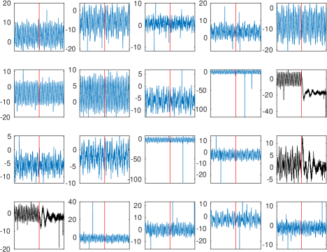
Figure 3: One instance of the $1000$ different synthetic datasets used in Sec. 4.3. The dimensions which exhibit a structural change can be seen in black. The data contain outliers and the true changepoint can be seen as marked by the vertical red line.

We generate data with $n=1200$ and use the data after the data point $n_{0}=400$ to estimate changepoints, as PSMF has to converge to a stable regime before it can be used to detect changepoints. The true changepoint is at $n_{c}=601$.

G.2.2 The GP subspace model

In this subsection, we provide the details of the discretization of the Matérn-$3/2$ SDE. Particularly, we consider the SDE Särkkä et al., (2013)

$$\frac{\,{\mathrm{d}}\mathsf{x}_{i}(t)}{\,{\mathrm{d}}t}=\mathsf{F}\mathsf{x}_{i}(t)+\begin{bmatrix}0\\ 1\end{bmatrix}w_{i}(t)$$ (G.6)

where $\mathsf{x}_{i}(t)=[x_{i}(t),\,{\mathrm{d}}x_{i}(t)/\,{\mathrm{d}}t]$ and $\kappa=\sqrt{2\nu}/{\ell}$ and

$$\mathsf{F}=\begin{bmatrix}0&1\\ -\kappa^{2}&-2\kappa\end{bmatrix}.$$ (G.7)

Given a step-size $\gamma$, the SDE (G.6) can be written as a linear dynamical system

$$x_{i,k}=A_{i}x_{i,k-1}+Q_{i}^{1/2}u_{i,k}$$ (G.8)

where $A_{i}=\textnormal{expm}(\gamma F)$ where expm denotes the matrix exponential and $Q_{i}=P_{\infty}-A_{i}P_{\infty}A_{i}^{\top}$ and

$$P_{\infty}=\begin{bmatrix}\sigma^{2}&0\\ 0&3\sigma^{2}/\ell^{2}\end{bmatrix}.$$ (G.9)

Finally, we construct our dynamical system as

$$x_{k}=Ax_{k-1}+Q^{1/2}u_{k}$$ (G.10)

where $x_{k}=[x_{1,k},\ldots,x_{r,k}]^{\top}\in{\mathbb{R}}^{2r}$ and

$$A=I_{r}\otimes A_{i}\quad\quad\textnormal{and}\quad\quad Q=I_{r}\otimes Q_{i}.$$ (G.11)

Using these system matrices, we define $H_{i}=[1,0]$ and $H=I_{r}\otimes H_{i}$ and finally define the probabilistic model

$$p(C) =\mathcal{MN}(C;C_{0},I_{d},V_{0}),$$ (G.12)

$$p(x_{0}) ={\mathcal{N}}(x_{0};\mu_{0},P_{0}),$$ (G.13)

$$p(x_{k}|x_{k-1}) ={\mathcal{N}}(x_{k};Ax_{k-1},Q),$$ (G.14)

$$p(y_{k}|x_{k},C) ={\mathcal{N}}(y_{k};CHx_{k},R).$$ (G.15)

Inference in this model can be done via a simple modification of the Algorithm 1 where $H$ matrix is involved in the computations. Fig. 4 illustrates the learned GP features $r=4$ and two change points.

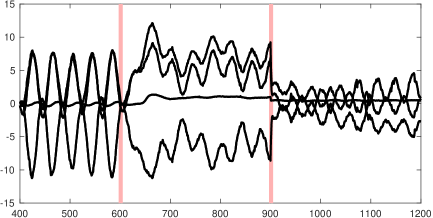
Figure 4: An illustration of the learned GP features vs. true changepoints for $r=4$ and two changepoints.

G.3 Experiment 3

All experiments where run on a Linux machine with an AMD Ryzen 5 3600 processor and 32GB of memory. Additional results on different missing percentages are shown in Table 4 and Table 5. We again observe excellent imputation performance of the proposed methods.

Table 4: Imputation error and runtime on several datasets using 20% and 40% missing values, averaged over 100 random repetitions. An asterisk marks offline methods.

(a) 20% missing data

	Imputation RMSE					Runtime (s)
	NO2	PM10	PM25	S&P500	Gas	NO2	PM10	PM25	S&P500	Gas
PSMF	$\underset{{\scriptscriptstyle(0.10)}}{\textbf{5.52}}$	$\underset{{\scriptscriptstyle(0.38)}}{\textbf{7.26}}$	$\underset{{\scriptscriptstyle(0.52)}}{3.42}$	$\underset{{\scriptscriptstyle(1.93)}}{9.95}$	$\underset{{\scriptscriptstyle(0.57)}}{\textbf{4.19}}$	2.71	2.59	1.92	9.42	101.16
rPSMF	$\underset{{\scriptscriptstyle(0.14)}}{5.53}$	$\underset{{\scriptscriptstyle(0.46)}}{7.47}$	$\underset{{\scriptscriptstyle(0.52)}}{\textbf{3.40}}$	$\underset{{\scriptscriptstyle(1.41)}}{\textbf{9.29}}$	$\underset{{\scriptscriptstyle(0.51)}}{4.56}$	2.91	2.73	2.03	13.98	122.57
MLE-SMF	$\underset{{\scriptscriptstyle\;\;(0.51)}}{11.03}$	$\underset{{\scriptscriptstyle(0.37)}}{9.46}$	$\underset{{\scriptscriptstyle(0.63)}}{4.81}$	$\underset{{\scriptscriptstyle\;\;(1.02)}}{30.23}$	$\underset{{\scriptscriptstyle\;\;(14.84)}}{87.12}$	2.48	2.39	1.71	9.52	92.09
TMF	$\underset{{\scriptscriptstyle(0.14)}}{7.60}$	$\underset{{\scriptscriptstyle(0.30)}}{7.95}$	$\underset{{\scriptscriptstyle(0.50)}}{4.43}$	$\underset{{\scriptscriptstyle\;\;(1.00)}}{34.96}$	$\underset{{\scriptscriptstyle\;\;(8.85)}}{73.70}$	1.03	0.97	0.72	4.19	35.35
PMF*	$\underset{{\scriptscriptstyle\;\;(0.08)}}{10.47}$	$\underset{{\scriptscriptstyle\;\;(0.26)}}{10.46}$	$\underset{{\scriptscriptstyle(0.48)}}{3.97}$	$\underset{{\scriptscriptstyle\;\;(1.80)}}{40.07}$	$\underset{{\scriptscriptstyle\;\;(0.06)}}{23.54}$	2.14	1.90	0.68	3.12	31.78
BPMF*	$\underset{{\scriptscriptstyle(0.18)}}{9.03}$	$\underset{{\scriptscriptstyle(0.28)}}{8.39}$	$\underset{{\scriptscriptstyle(0.49)}}{3.61}$	$\underset{{\scriptscriptstyle\;\;(0.93)}}{27.36}$	$\underset{{\scriptscriptstyle\;\;(0.17)}}{17.70}$	3.11	4.48	3.05	4.15	92.50

(b) 40% missing data

	Imputation RMSE					Runtime (s)
	NO2	PM10	PM25	S&P500	Gas	NO2	PM10	PM25	S&P500	Gas
PSMF	$\underset{{\scriptscriptstyle(0.18)}}{6.06}$	$\underset{{\scriptscriptstyle(0.28)}}{7.72}$	$\underset{{\scriptscriptstyle(0.23)}}{3.77}$	$\underset{{\scriptscriptstyle\;\;(3.06)}}{13.87}$	$\underset{{\scriptscriptstyle(1.63)}}{\textbf{8.75}}$	2.77	2.62	1.92	9.12	100.68
rPSMF	$\underset{{\scriptscriptstyle(0.27)}}{\textbf{5.96}}$	$\underset{{\scriptscriptstyle(0.57)}}{\textbf{7.68}}$	$\underset{{\scriptscriptstyle(0.29)}}{\textbf{3.67}}$	$\underset{{\scriptscriptstyle\;\;(4.39)}}{\textbf{12.36}}$	$\underset{{\scriptscriptstyle(2.28)}}{9.03}$	2.92	2.77	2.02	13.30	109.38
MLE-SMF	$\underset{{\scriptscriptstyle\;\;(0.49)}}{11.30}$	$\underset{{\scriptscriptstyle(0.30)}}{9.55}$	$\underset{{\scriptscriptstyle(0.31)}}{4.93}$	$\underset{{\scriptscriptstyle\;\;(0.80)}}{30.14}$	$\underset{{\scriptscriptstyle\;\;\;(26.65)}}{125.54}$	2.54	2.38	1.70	9.59	85.11
TMF	$\underset{{\scriptscriptstyle(0.12)}}{7.90}$	$\underset{{\scriptscriptstyle(0.21)}}{8.27}$	$\underset{{\scriptscriptstyle(0.31)}}{4.86}$	$\underset{{\scriptscriptstyle\;\;(0.76)}}{34.78}$	$\underset{{\scriptscriptstyle\;\;(10.60)}}{66.27}$	0.98	0.97	0.73	4.13	32.01
PMF*	$\underset{{\scriptscriptstyle\;\;(0.05)}}{10.54}$	$\underset{{\scriptscriptstyle\;\;(0.15)}}{10.53}$	$\underset{{\scriptscriptstyle(0.13)}}{4.11}$	$\underset{{\scriptscriptstyle\;\;(1.81)}}{41.53}$	$\underset{{\scriptscriptstyle\;\;(0.06)}}{24.12}$	1.73	1.51	0.54	2.43	24.75
BPMF*	$\underset{{\scriptscriptstyle(0.21)}}{9.46}$	$\underset{{\scriptscriptstyle(0.18)}}{8.64}$	$\underset{{\scriptscriptstyle(0.12)}}{3.72}$	$\underset{{\scriptscriptstyle\;\;(0.64)}}{27.91}$	$\underset{{\scriptscriptstyle\;\;(0.37)}}{19.10}$	4.26	4.07	2.92	3.16	82.44

Table 5: Average coverage proportion of the missing data by the $2\sigma$ uncertainty bars of the posterior predictive estimates for 20% and 40% missing values, averaged over 100 repetitions.

(a) 20% missing data

	NO2	PM10	PM25	S&P500	Gas
PSMF	0.79	0.79	0.93	0.85	0.93
rPSMF	0.89	0.92	0.91	0.86	0.90
MLE-SMF	0.46	0.59	0.83	0.51	0.61

(b) 40% missing data

	NO2	PM10	PM25	S&P500	Gas
PSMF	0.71	0.73	0.89	0.78	0.83
rPSMF	0.79	0.84	0.81	0.79	0.79
MLE-SMF	0.40	0.53	0.77	0.44	0.49

Appendix H CONVERGENCE DISCUSSION

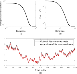
Figure 5: (a) Convergence of the approximate posterior and true posterior (with true $C^{\star}$) in averaged Wasserstein distance for iterative PSMF. (b) Convergence of the mean $C_{k}$ to $C^{\star}$. (c) Filter estimates given by the iterative PSMF and the optimal filter.

To gain insights in the convergence of our method, we have designed a simplified setup where the latent state trajectory is a one-dimensional random walk and observations are four-dimensional, and we have simulated a dataset consisting of size 1,000 where $C\in{\mathbb{R}}^{4}$. We run the KF with the ground-truth value $C^{\star}$. We also run the iterative PSMF which also estimates $C$ as well as the hidden states. We have computed the distance between the sequence of optimal (Gaussian) filters constructed by the KF and the filters of the iterative PSMF in terms of the averaged Wasserstein distance over the path:

$${\overline{W}_{2}}(t):=\frac{1}{t}\sum_{k=1}^{t}W_{2}(p_{\star}(x_{k}|y_{1:k}),\tilde{p}(x_{k}|y_{1:k})).$$ (H.1)

We observe that the distance between the optimal and approximate filters over the entire path is uniformly bounded (see Fig. 5(a)). We also observe that $C_{k}\to C^{\star}$ for this case, see Fig. 5(b) and show the mean estimates are sufficiently close (Fig. 5(c)).

More precisely, we simulate the following state-space model

$$p(x_{0}) ={\mathcal{N}}(x_{0};\mu_{0},P_{0}),$$ (H.2)

$$p(x_{k}|x_{k-1}) ={\mathcal{N}}(x_{k};x_{k-1},Q),$$ (H.3)

$$p(y_{k}|x_{k},C^{\star}) ={\mathcal{N}}(y_{k};C^{\star}x_{k},R),$$ (H.4)

where $C^{\star}\in{\mathbb{R}}^{4}$ and $x_{k}\in{\mathbb{R}}$, which leads to $y_{k}\in{\mathbb{R}}^{4}$. In this case, the identifability problem is alleviated since $C^{\star}$ is a vector and we can test empirically whether the posterior provided by the PSMF for the states $p(x_{k}|y_{1:k})$ converges to the true posterior of the states $p_{\star}(x_{k}|y_{1:k})$.

Note that, the PSMF provides the filtering distribution of states as a Gaussian

$$\tilde{p}(x_{k}|y_{1:k})={\mathcal{N}}(x_{k};\mu_{k},P_{k})$$ (H.5)

where $\mu_{k},P_{k}$ are defined within Algorithm 1. Since the data is generated from the model using $C^{\star}$, we also compute the optimal Kalman filter with $C^{\star}$ which we denote as $p_{\star}(x_{k}|y_{1:k})$. In order to test the convergence between the approximate filter provided by the PSMF $\tilde{p}(x_{k}|y_{1:k})$ and the true filter $p_{\star}(x_{k}|y_{1:k})$, we use the Wasserstein-2 distance which is defined as

$$W_{2}(\mu,\nu)=\inf_{\Gamma\in\mathcal{C}(\mu,\nu)}\iint\|x-y\|^{2}\Gamma(\,{\mathrm{d}}x,\,{\mathrm{d}}y)$$ (H.6)

where $\mathcal{C}(\mu,\nu)$ is the set of couplings whose marginals are $\mu$ and $\nu$ respectively. This Wasserstein-2 distance can be computed in closed form for two Gaussians, e.g., for $\mu={\mathcal{N}}(\mu_{1},\Sigma_{1})$ and $\nu={\mathcal{N}}(\mu_{2},\Sigma_{2})$, we have

$$W_{2}(\mu,\nu)^{2}=\|\mu_{1}-\mu_{2}\|^{2}+{\operatorname{Tr}}(\Sigma_{1}+\Sigma_{2}-2(\Sigma_{2}^{1/2}\Sigma_{1}\Sigma_{2}^{1/2})^{1/2}).$$ (H.7)

Hence, for a given sequence of filters $(\tilde{p}(x_{k}|y_{1:k}))_{k\geq 1}$ and $(p_{\star}(x_{k}|y_{1:k}))_{k\geq 1}$, we define the averaged Wasserstein distance for time $t$ as

$$\overline{W}_{2}(t)=\frac{1}{t}\sum_{k=1}^{t}W_{2}(\tilde{p}(x_{k}|y_{1:k}),{p}_{\star}(x_{k}|y_{1:k})).$$ (H.8)

One can see from Fig. 5 that $\lim_{t\to\infty}\overline{W}_{2}(t)<\infty$ which implies that a convergence result can be proven for our method. We leave this exciting direction to future work.

Appendix I ADDITIONAL RESULTS FOR RECURSIVE PSMF

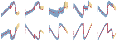
Figure 6: Recursive PSMF. Observed time series (blue) with unobserved future data (yellow) and the reconstruction from the model (red).

In this section, we present an additional result using recursive PSMF to demonstrate the scalability of our method in a purely streaming setting.

Using the same setting of Sec. 4.1, we use a longer sequence ($n=4000$) with an additional prediction sequence of length $800$. This presents a challenging setting as we do not iterate over data and the algorithm observes the training data only once (i.e. the streaming setting). As can be seen from Fig. 6, recursive PSMF learns the underlying dynamics and has a successful out-of-sample prediction performance, even with a relatively long sequence into the future. This demonstrates the recursive version of our method can be used in a setting where iterating over data multiple times is impractical.

References

- Adams and MacKay, (2007) Adams, R. P. and MacKay, D. J. (2007). Bayesian online changepoint detection. arXiv preprint arXiv:0710.3742.
- Akyildiz and Míguez, (2019) Akyildiz, Ö. D. and Míguez, J. (2019). Dictionary filtering: a probabilistic approach to online matrix factorisation. Signal, Image and Video Processing, 13(4):737–744.
- Anderson and Moore, (1979) Anderson, B. D. and Moore, J. B. (1979). Optimal filtering. Englewood Cliffs, N.J. Prentice Hall.
- Andrieu et al., (2010) Andrieu, C., Doucet, A., and Holenstein, R. (2010). Particle Markov chain Monte Carlo methods. Journal of the Royal Statistical Society: Series B (Statistical Methodology), 72(3):269–342.
- Andrieu et al., (2005) Andrieu, C., Doucet, A., and Tadic, V. B. (2005). On-line parameter estimation in general state-space models. In Proceedings of the 44th IEEE Conference on Decision and Control, pages 332–337. IEEE.
- Ayed et al., (2019) Ayed, I., de Bézenac, E., Pajot, A., Brajard, J., and Gallinari, P. (2019). Learning dynamical systems from partial observations. arXiv preprint arXiv:1902.11136.
- Bache and Lichman, (2013) Bache, K. and Lichman, M. (2013). UCI machine learning repository.
- Basu and Das, (1994) Basu, A. K. and Das, J. K. (1994). A Bayesian approach to Kalman filter for elliptically contoured distribution and its application in time series models. Calcutta Statistical Association Bulletin, 44(1-2):11–28.
- Bengtsson et al., (2008) Bengtsson, T., Bickel, P., Li, B., et al. (2008). Curse-of-dimensionality revisited: Collapse of the particle filter in very large scale systems. In Probability and statistics: Essays in honor of David A. Freedman, pages 316–334. Institute of Mathematical Statistics.
- Berry et al., (2007) Berry, M. W., Browne, M., Langville, A. N., Pauca, V. P., and Plemmons, R. J. (2007). Algorithms and applications for approximate nonnegative matrix factorization. Computational Statistics & Data Analysis, 52(1):155–173.
- Bishop, (2006) Bishop, C. M. (2006). Pattern Recognition and Machine Learning. Springer-Verlag New York, Inc., Secaucus, NJ, USA.
- Boots et al., (2008) Boots, B., Gordon, G. J., and Siddiqi, S. M. (2008). A constraint generation approach to learning stable linear dynamical systems. In Advances in neural information processing systems, pages 1329–1336.
- Bucak and Günsel, (2009) Bucak, S. S. and Günsel, B. (2009). Incremental subspace learning via non-negative matrix factorization. Pattern Recognition, 42(5):788–797.
- Burgués et al., (2018) Burgués, J., Jiménez-Soto, J. M., and Marco, S. (2018). Estimation of the limit of detection in semiconductor gas sensors through linearized calibration models. Analytica Chimica Acta, 1013:13–25.
- Cai et al., (2010) Cai, D., He, X., Han, J., and Huang, T. S. (2010). Graph regularized nonnegative matrix factorization for data representation. IEEE transactions on Pattern Analysis and Machine Intelligence, 33(8):1548–1560.
- Cappé, (2011) Cappé, O. (2011). Online EM algorithm for hidden Markov models. Journal of Computational and Graphical Statistics, 20(3):728–749.
- Cappé and Moulines, (2009) Cappé, O. and Moulines, E. (2009). On-line expectation–maximization algorithm for latent data models. Journal of the Royal Statistical Society: Series B (Statistical Methodology), 71(3):593–613.
- Cemgil, (2009) Cemgil, A. T. (2009). Bayesian inference for nonnegative matrix factorisation models. Computational Intelligence and Neuroscience, pages 4:1–4:17.
- Ding et al., (2008) Ding, C. H., Li, T., and Jordan, M. I. (2008). Convex and semi-nonnegative matrix factorizations. IEEE transactions on pattern analysis and machine intelligence, 32(1):45–55.
- Douc et al., (2011) Douc, R., Moulines, E., Olsson, J., Van Handel, R., et al. (2011). Consistency of the maximum likelihood estimator for general hidden Markov models. the Annals of Statistics, 39(1):474–513.
- Doucet et al., (2000) Doucet, A., Godsill, S., and Andrieu, C. (2000). On sequential Monte Carlo sampling methods for Bayesian filtering. Statistics and computing, 10(3):197–208.
- Elliott and Krishnamurthy, (1999) Elliott, R. J. and Krishnamurthy, V. (1999). New finite-dimensional filters for parameter estimation of discrete-time linear Gaussian models. IEEE Transactions on Automatic Control, 44(5):938–951.
- Fernandez-Bes et al., (2015) Fernandez-Bes, J., Elvira, V., and Van Vaerenbergh, S. (2015). A probabilistic least-mean-squares filter. In IEEE International Conference on Acoustics, Speech and Signal Processing (ICASSP), pages 2199–2203. IEEE.
- Févotte and Idier, (2011) Févotte, C. and Idier, J. (2011). Algorithms for nonnegative matrix factorization with the -divergence. Neural computation, 23(9):2421–2456.
- Févotte et al., (2013) Févotte, C., Le Roux, J., and Hershey, J. R. (2013). Non-negative dynamical system with application to speech and audio. In 2013 IEEE International Conference on Acoustics, Speech and Signal Processing, pages 3158–3162. IEEE.
- Févotte et al., (2018) Févotte, C., Smaragdis, P., Mohammadiha, N., and Mysore, G. J. (2018). Temporal extensions of nonnegative matrix factorization. Audio Source Separation and Speech Enhancement, pages 161–187.
- Gemulla et al., (2011) Gemulla, R., Nijkamp, E., Haas, P. J., and Sismanis, Y. (2011). Large-scale matrix factorization with distributed stochastic gradient descent. In Proceedings of the 17th ACM SIGKDD international conference on Knowledge discovery and data mining, pages 69–77. ACM.
- Ghahramani and Hinton, (1996) Ghahramani, Z. and Hinton, G. E. (1996). Parameter estimation for linear dynamical systems. Technical Report CRG-TR-96-2, University of Toronto, Dept. of Computer Science.
- Girón and Rojano, (1994) Girón, F. and Rojano, J. (1994). Bayesian Kalman filtering with elliptically contoured errors. Biometrika, 81(2):390–395.
- Gupta and Nagar, (1999) Gupta, A. K. and Nagar, D. K. (1999). Matrix variate distributions, volume 104. CRC Press.
- Hartikainen and Särkkä, (2010) Hartikainen, J. and Särkkä, S. (2010). Kalman filtering and smoothing solutions to temporal Gaussian process regression models. In 2010 IEEE International Workshop on Machine Learning for Signal Processing, pages 379–384. IEEE.
- Harville, (1997) Harville, D. A. (1997). Matrix algebra from a statistician’s perspective, volume 1. Springer.
- Julier and Uhlmann, (1997) Julier, S. J. and Uhlmann, J. K. (1997). New extension of the Kalman filter to nonlinear systems. In Signal processing, sensor fusion, and target recognition VI, volume 3068, pages 182–193. International Society for Optics and Photonics.
- Kalman, (1960) Kalman, R. E. (1960). A new approach to linear filtering and prediction problems. Journal of Basic Engineering, 82(1):35–45.
- Kantas et al., (2015) Kantas, N., Doucet, A., Singh, S. S., Maciejowski, J., and Chopin, N. (2015). On particle methods for parameter estimation in state-space models. Statistical Science, 30(3):328–351.
- Karami et al., (2017) Karami, M., White, M., Schuurmans, D., and Szepesvári, C. (2017). Multi-view matrix factorization for linear dynamical system estimation. In Advances in Neural Information Processing Systems, pages 7092–7101.
- Katayama, (2006) Katayama, T. (2006). Subspace methods for system identification. Springer Science & Business Media.
- Killick et al., (2012) Killick, R., Fearnhead, P., and Eckley, I. A. (2012). Optimal detection of changepoints with a linear computational cost. Journal of the American Statistical Association, 107(500):1590–1598.
- Kingma and Ba, (2015) Kingma, D. P. and Ba, J. (2015). Adam: A method for stochastic optimization. In International Conference on Learning Representations (ICLR).
- Lee and Seung, (1999) Lee, D. D. and Seung, H. S. (1999). Learning the parts of objects by non-negative matrix factorization. Nature, 401(6755):788–791.
- Lee and Seung, (2001) Lee, D. D. and Seung, H. S. (2001). Algorithms for non-negative matrix factorization. In Advances in neural information processing systems, pages 556–562.
- Liang et al., (2015) Liang, X., Zou, T., Guo, B., Li, S., Zhang, H., Zhang, S., Huang, H., and Chen, S. X. (2015). Assessing Beijing’s PM2.5 pollution: severity, weather impact, APEC and winter heating. Proceedings of the Royal Society A: Mathematical, Physical and Engineering Sciences, 471(2182):20150257.
- Lin, (2007) Lin, C.-J. (2007). Projected gradient methods for nonnegative matrix factorization. Neural computation, 19(10):2756–2779.
- Liu and Hauskrecht, (2016) Liu, Z. and Hauskrecht, M. (2016). Learning linear dynamical systems from multivariate time series: A matrix factorization based framework. In Proceedings of the 2016 SIAM International Conference on Data Mining, pages 810–818. SIAM.
- Mairal et al., (2010) Mairal, J., Bach, F., Ponce, J., and Sapiro, G. (2010). Online learning for matrix factorization and sparse coding. The Journal of Machine Learning Research, 11:19–60.
- McLean et al., (1962) McLean, J. D., Schmidt, S. F., and McGee, L. A. (1962). Optimal filtering and linear prediction applied to a midcourse navigation system for the circumlunar mission. Technical Report D-1208, National Aeronautics and Space Administration.
- Mensch et al., (2016) Mensch, A., Mairal, J., Thirion, B., and Varoquaux, G. (2016). Dictionary learning for massive matrix factorization. In International Conference on Machine Learning, pages 1737–1746.
- Mnih and Salakhutdinov, (2008) Mnih, A. and Salakhutdinov, R. R. (2008). Probabilistic matrix factorization. In Advances in neural information processing systems, pages 1257–1264.
- Mohammadiha et al., (2013) Mohammadiha, N., Smaragdis, P., and Leijon, A. (2013). Prediction based filtering and smoothing to exploit temporal dependencies in NMF. In 2013 IEEE International Conference on Acoustics, Speech and Signal Processing, pages 873–877. IEEE.
- Mohammadiha et al., (2014) Mohammadiha, N., Smaragdis, P., Panahandeh, G., and Doclo, S. (2014). A state-space approach to dynamic nonnegative matrix factorization. IEEE Transactions on Signal Processing, 63(4):949–959.
- Ozerov and Févotte, (2009) Ozerov, A. and Févotte, C. (2009). Multichannel nonnegative matrix factorization in convolutive mixtures for audio source separation. IEEE Transactions on Audio, Speech, and Language Processing, 18(3):550–563.
- Paisley et al., (2014) Paisley, J. W., Blei, D. M., and Jordan, M. I. (2014). Bayesian nonnegative matrix factorization with stochastic variational inference. In Handbook of Mixed Membership Models and Their Applications. Chapman & Hall/CRC.
- Rennie and Srebro, (2005) Rennie, J. D. M. and Srebro, N. (2005). Fast maximum margin matrix factorization for collaborative prediction. In Proceedings of the 22nd International Conference on Machine Learning, pages 713–719.
- Roth, (2012) Roth, M. (2012). On the multivariate t distribution. Technical Report LiTH-ISY-R-3059, Linköping University.
- Roth et al., (2017) Roth, M., Ardeshiri, T., Özkan, E., and Gustafsson, F. (2017). Robust Bayesian filtering and smoothing using Student’s t distribution. arXiv preprint arXiv:1703.02428.
- Roth et al., (2013) Roth, M., Özkan, E., and Gustafsson, F. (2013). A Student’s t filter for heavy tailed process and measurement noise. In IEEE International Conference on Acoustics, Speech and Signal Processing, pages 5770–5774. IEEE.
- Salakhutdinov and Mnih, (2008) Salakhutdinov, R. and Mnih, A. (2008). Bayesian probabilistic matrix factorization using Markov chain Monte Carlo. In Proceedings of the 25th international conference on Machine learning, pages 880–887. ACM.
- Särkkä, (2013) Särkkä, S. (2013). Bayesian filtering and smoothing. Cambridge University Press.
- Särkkä et al., (2013) Särkkä, S., Solin, A., and Hartikainen, J. (2013). Spatiotemporal learning via infinite-dimensional Bayesian filtering and smoothing: A look at Gaussian process regression through Kalman filtering. IEEE Signal Processing Magazine, 30(4):51–61.
- Schmidt et al., (2009) Schmidt, M. N., Winther, O., and Hansen, L. K. (2009). Bayesian non-negative matrix factorization. In International Conference on Independent Component Analysis and Signal Separation, pages 540–547. Springer.
- Shahnaz et al., (2006) Shahnaz, F., Berry, M. W., Pauca, V. P., and Plemmons, R. J. (2006). Document clustering using nonnegative matrix factorization. Information Processing & Management, 42(2):373–386.
- Shi et al., (2016) Shi, W., Zhu, Y., Philip, S. Y., Huang, T., Wang, C., Mao, Y., and Chen, Y. (2016). Temporal dynamic matrix factorization for missing data prediction in large scale coevolving time series. IEEE Access, 4:6719–6732.
- Smaragdis and Brown, (2003) Smaragdis, P. and Brown, J. C. (2003). Non-negative matrix factorization for polyphonic music transcription. In 2003 IEEE Workshop on Applications of Signal Processing to Audio and Acoustics (IEEE Cat. No. 03TH8684), pages 177–180. IEEE.
- Snyder et al., (2008) Snyder, C., Bengtsson, T., Bickel, P., and Anderson, J. (2008). Obstacles to high-dimensional particle filtering. Monthly Weather Review, 136(12):4629–4640.
- Sun et al., (2012) Sun, J. Z., Varshney, K. R., and Subbian, K. (2012). Dynamic matrix factorization: A state space approach. In Acoustics, Speech and Signal Processing (ICASSP), 2012 IEEE International Conference on, pages 1897–1900. IEEE.
- Tronarp et al., (2019) Tronarp, F., Karvonen, T., and Särkkä, S. (2019). Student’s -filters for noise scale estimation. IEEE Signal Processing Letters, 26(2):352–356.
- Wang et al., (2012) Wang, N., Yao, T., Wang, J., and Yeung, D.-Y. (2012). A probabilistic approach to robust matrix factorization. In European Conference on Computer Vision, pages 126–139. Springer.
- White et al., (2015) White, M., Wen, J., Bowling, M., and Schuurmans, D. (2015). Optimal estimation of multivariate ARMA models. In Twenty-Ninth AAAI Conference on Artificial Intelligence.
- Williams and Rasmussen, (2006) Williams, C. K. and Rasmussen, C. E. (2006). Gaussian processes for machine learning. MIT press Cambridge, MA, 2nd edition.
- Woodbury, (1950) Woodbury, M. A. (1950). Inverting modified matrices. Statistical Research Group Memorandum Report 42, Princeton University.
- Yildirim et al., (2012) Yildirim, S., Cemgil, A. T., and Singh, S. S. (2012). An online expectation-maximisation algorithm for nonnegative matrix factorisation models. IFAC Proceedings Volumes, 45(16):494–499.
- Yu et al., (2016) Yu, H.-F., Rao, N., and Dhillon, I. S. (2016). Temporal regularized matrix factorization for high-dimensional time series prediction. In Advances in Neural Information Processing Systems, pages 847–855.
- Zheng et al., (2013) Zheng, X., Ding, H., Mamitsuka, H., and Zhu, S. (2013). Collaborative matrix factorization with multiple similarities for predicting drug-target interactions. In Proceedings of the 19th ACM SIGKDD international conference on Knowledge discovery and data mining, pages 1025–1033.