Flexible distribution-free conditional predictive bands
using density estimators

Abstract

Conformal methods create prediction bands that control average coverage under no assumptions besides i.i.d. data. Besides average coverage, one might also desire to control conditional coverage, that is, coverage for every new testing point. However, without strong assumptions, conditional coverage is unachievable. Given this limitation, the literature has focused on methods with asymptotical conditional coverage. In order to obtain this property, these methods require strong conditions on the dependence between the target variable and the features. We introduce two conformal methods based on conditional density estimators that do not depend on this type of assumption to obtain asymptotic conditional coverage: Dist-split and CD-split. While Dist-split asymptotically obtains optimal intervals, which are easier to interpret than general regions, CD-split obtains optimal size regions, which are smaller than intervals. CD-split also obtains local coverage by creating a data-driven partition of the feature space that scales to high-dimensional settings and by generating prediction bands locally on the partition elements. In a wide variety of simulated scenarios, our methods have a better control of conditional coverage and have smaller length than previously proposed methods.

1 Introduction

Supervised machine learning methods predict a response variable, $Y\in{\mathcal{Y}}$, based on features, ${\mathbf{X}}\in{\mathcal{X}}$, using an i.i.d. sample, $({\mathbf{X}}_{1},Y_{1}),\ldots,({\mathbf{X}}_{n},Y_{n})$. While most methods yield point estimates, it is often more informative to present prediction bands, that is, a subset of ${\mathcal{Y}}$ with plausible values for $Y$ (Neter et al.,, 1996).

A particular way of constructing prediction bands is through conformal predictions (Vovk et al.,, 2005, 2009). This methodology is appealing because it controls the marginal coverage of the prediction bands assuming solely i.i.d. data. Specifically, given a new instance, $({\mathbf{X}}_{n+1},Y_{n+1})$, a conformal prediction, $C({\mathbf{X}}_{n+1})$, satisfies

$${\mathbb{P}}\left(Y_{n+1}\in C({\mathbf{X}}_{n+1})\right) \geq 1-\alpha,$$

where $0<1-\alpha<1$ is a desired coverage level. Besides marginal validity one might also wish for stronger guarantees. For instance, conditional validity holds when, for every ${\mathbf{x}}_{n+1}\in{\mathcal{X}}$,

$${\mathbb{P}}(Y_{n+1}\in C(\textbf{X}_{n+1})|\textbf{X}_{n+1}=\textbf{x}_{n+1}) \geq 1-\alpha.$$

That is, conditional validity guarantees adequate coverage for each new instance and not solely on average across instances.

Unfortunately, conditional validity can be obtained only under strong assumptions about the the distribution of $({\mathbf{X}},Y)$ (Vovk,, 2012; Lei and Wasserman,, 2014; Barber et al.,, 2019). Given this result, effort has been focused on obtaining intermediate conditions. For instance, many conformal methods control local coverage:

$${\mathbb{P}}(Y_{n+1}\in C(\textbf{X}_{n+1})|\textbf{X}_{n+1}\in A) \geq 1-\alpha,$$

where $A$ is a subset of $\mathcal{X}$ (Lei and Wasserman,, 2014; Barber et al.,, 2019; Guan,, 2019). These methods are based on computing conformal bands using only instances that fall in $A$. However, to date, these methods do not scale to high-dimensional settings because it is challenging to create $A$ that is large enough so that many instances fall in $A$, and yet small enough so that

$${\mathbb{P}}(Y_{n+1}\in C(\textbf{X}_{n+1})|\textbf{X}_{n+1}\in A)\approx{\mathbb{P}}(Y_{n+1}\in C(\textbf{X}_{n+1})|\textbf{X}_{n+1}={\mathbf{x}}_{n+1}),$$

that is, local validity is close to conditional validity.

Another alternative to conditional validity is asymptotic conditional coverage (Lei et al.,, 2018). Under this property, conditional coverage converges to the specified level as the sample size increases. That is, there exist random sets, $\Lambda_{n}$, such that ${\mathbb{P}}(X_{n+1}\in\Lambda_{n}|\Lambda_{n})=1-o_{P}(1)$ and

$$\sup_{x\in\Lambda_{n}}\big{|}{\mathbb{P}}(Y_{n+1}\in C(\textbf{X}_{n+1})|\textbf{X}_{n+1}={\mathbf{x}}_{n+1})-1-\alpha\big{|}=o_{P}(1).$$

In a regression context in which ${\mathcal{Y}}=\mathbb{R}$, Lei et al., (2018) obtains asymptotic conditional coverage under assumptions such as $Y=\mu({\mathbf{X}})+\epsilon$, where $\epsilon$ is independent of ${\mathbf{X}}$ and has density symmetric around 0. Furthermore, the proposed prediction band converges to the interval with the smallest interval among the ones with adequate conditional coverage.

Despite the success of these methods, there exists space for improvement. In many problems the assumption that $\epsilon$ is independent of ${\mathbf{X}}$ and has a density symmetric around $0$ is unrealistic. For instance, in heteroscedastic settings (Neter et al.,, 1996), $\epsilon$ depends on ${\mathbf{X}}$. It is also common for $\epsilon$ to have an asymmetric or even multimodal distribution. Furthermore, in these general settings, the smallest region with adequate conditional coverage might not be an interval, which is the outcome of most current methods.

1.1 Contribution

We propose new methods and show that they obtain asymptotic conditional coverage without assuming a particular type of dependence between the target and the features. Specifically, we propose two methods: Dist-split and CD-split. While Dist-split produces prediction bands that are intervals and easier to interpret, CD-split yields arbitrary regions, which are generally smaller and appealing for multimodal data. While Dist-split converges to an oracle interval, CD-split converges to an oracle region. Furthermore, since CD-split is based on a novel data-driven way of partitioning the feature space, it also controls local coverage even in high-dimensional settings. Table 1 summarizes the properties of these methods.

Table 1: Properties of Dist-split and CD-split.

Method	Marginal coverage	Asymptotic conditional coverage	Local coverage	Prediction bands are intervals	Can be used for classification?
Dist-split	✓	✓	✗	✓	✗
CD-split	✓	✓	✓	✗	✓

The proposed methods also have desirable computational properties. They are based on fast-to-compute split (inductive)-conformal bands (Papadopoulos,, 2008; Vovk,, 2012; Lei et al.,, 2018) and on novel conditional density estimation methods that scale to high-dimensional datasets (Lueckmann et al.,, 2017; Papamakarios et al.,, 2017; Izbicki and Lee,, 2017) Both methods are easy to compute and scale to large sample sizes as long as the conditional density estimator also does.

In a wide variety of simulation studies, we show that our proposed methods obtain better conditional coverage and smaller band length than alternatives in the literature. For example, Figure 1 illustrates CD-split, Dist-split and the reg-split method from Lei et al., (2018) on the toy example from Lei and Wasserman, (2014). The bottom right plot shows that both CD-split and Dist-split get close to controlling conditional coverage. Since Dist-split can yield only intervals, CD-split obtains smaller bands in the region in which ${\mathbf{Y}}$ is bimodal. In this region CD-split yields a collection of intervals around each of the modes.

(a)

(b)

(c)

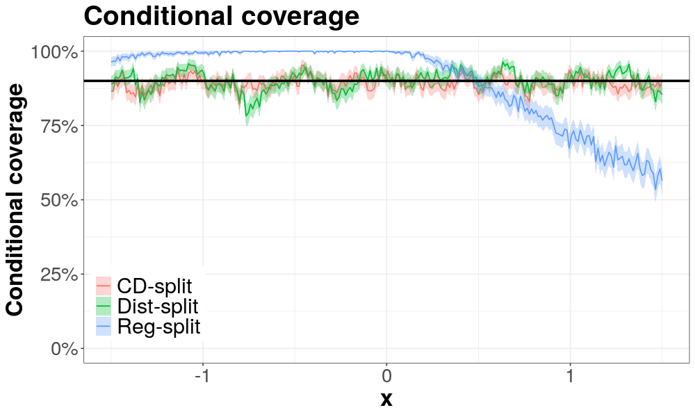
(d)

Figure 1: Comparison between CD-split, Dist-split and the reg-split method from Lei et al., (2018).

The remaining of the paper is organized as follows. Section 2 presents Dist-split. Section 3 presents CD-split. Experiments are shown in Section 4. Final remarks are on Section 5. All proofs are shown in the supplementary material.

Notation. Unless stated otherwise, we study a univariate regression setting such that ${\mathcal{Y}}={\mathbb{R}}$. Data from an i.i.d. sequence is split into two parts, $\mathbb{D}=\{({\mathbf{X}}_{1},Y_{1}),\ldots,({\mathbf{X}}_{n},Y_{n})\}$ and $\mathbb{D}^{\prime}=\{({\mathbf{X}}^{\prime}_{1},Y^{\prime}_{1}),\ldots,({\mathbf{X}}^{\prime}_{n},Y^{\prime}_{n})\}$. The assumption that both datasets have the same size is used solely to simplify notation. Also, the new instance, $({\mathbf{X}}_{n+1},Y_{n+1})$, has the same distribution as the other sample units. Finally, $q(\alpha;\{t_{1},\ldots,t_{m}\})$ is the $\alpha$ quantile of $\{t_{1},\ldots,t_{m}\}$.

2 Dist-split

The Dist-split method is based on the fact that, if $F(y|{\mathbf{x}})$ is the conditional distribution of ${Y_{n+1}}$ given ${{\mathbf{X}}_{n+1}}$, then $F({Y_{n+1}}|{{\mathbf{X}}_{n+1}})$ has uniform distribution. Therefore, if ${\widehat{F}}$ is close to $F$, then ${\widehat{F}}({Y_{n+1}}|{{\mathbf{X}}_{n+1}})$ approximately uniform, and does not depend on ${{\mathbf{X}}_{n+1}}$. That is, obtaining marginal coverage for ${\widehat{F}}({Y_{n+1}}|{{\mathbf{X}}_{n+1}})$ is close to obtaining conditional coverage.

Definition 2.1 (Dist-split prediction band).

Let ${\widehat{F}}(y|{\mathbf{x}}_{n+1})$ be an estimate based on $\mathbb{D}^{\prime}$ of the conditional distribution of $Y_{n+1}$ given ${\mathbf{x}}_{n+1}$. The Dist-split prediction band, $C\left({\mathbf{x}}_{n+1}\right)$, is

$$C \left({\mathbf{x}}_{n+1}\right):=\left\{y:q(.5\alpha;\mathcal{T}(\mathbb{D}))\leq{\widehat{F}}(y|{\mathbf{x}}_{n+1})\leq q(1-.5\alpha;\mathcal{T}(\mathbb{D}))\right\}$$

$$=\left[{\widehat{F}}^{-1}\left(q(.5\alpha;\mathcal{T}(\mathbb{D}))|{\mathbf{x}}_{n+1}\right);{\widehat{F}}^{-1}\left(q(1-.5\alpha;\mathcal{T}(\mathbb{D}))|{\mathbf{x}}_{n+1}\right)\right]$$

where $\mathcal{T}(\mathbb{D})=\left\{{\widehat{F}}(Y_{i}|{\mathbf{X}}_{i}),i=1,\ldots,n\right\}$.

Algorithm 1 shows an implementation of Dist-split.

Algorithm 1 Dist-split

Input: Data $(\textbf{X}_{i},Y_{i})$, $i=1,...,n$, miscoverage level $\alpha\in(0,1)$, algorithm $\mathcal{B}$ for fitting conditional cumulative distribution function
Output: Prediction band for $\textbf{x}_{n+1}\in\mathbb{R}^{d}$

1:  Randomly split $\{1,2,...,n\}$ into two subsets $\mathbb{D}$ e $\mathbb{D}^{\prime}$

2:  Fit $\hat{F}=\mathcal{B}(\{(\textbf{X}_{i},Y_{i}):i\in\mathbb{D}^{\prime}\})$  // Estimate cumulative distribution function

3:  Let $\mathcal{T}(\mathbb{D})=\{\hat{F}(y_{i}|\textbf{x}_{i}),i\in\mathbb{D}\}$

4:  Let $t_{1}=q(\alpha/2;\mathcal{T}(\mathbb{D}))$ and $t_{2}=q(1-\alpha/2;\mathcal{T}(\mathbb{D}))$  // Compute the quantiles of the set $\mathcal{T}(\mathbb{D})$

5:  return $\left\{y:t_{2}\geq\widehat{F}(y|\textbf{x}_{n+1})\geq t_{1}\right\}$

Dist-split adequately controls the marginal coverage. Furthermore, it exceeds the specified $1-\alpha$ coverage by at most $(n+1)^{-1}$. These results are presented in Theorem 2.2.

Theorem 2.2 (Marginal coverage).

Let $C(\textbf{X}_{n+1})$ be such as in Definition 2.1. If both $F(y|{\mathbf{x}})$ and ${\widehat{F}}(y|{\mathbf{x}})$ are continuous for every ${\mathbf{x}}\in\mathcal{X}$, then

$$1-\alpha\leq\mathbb{P}(Y_{n+1}\in C(\textbf{X}_{n+1}))\leq 1-\alpha+\frac{1}{n+1}.$$

Under additional assumptions Dist-split also obtains asymptotic conditional coverage and converges to an optimal oracle band. Two types of assumptions are required. First, that the conditional density estimator, ${\widehat{F}}$ is consistent. This assumption is an adaptation to density estimators of the consistency assumption for regression estimators in (Lei et al.,, 2018). Also, we require that $F(y|{\mathbf{x}})$ is differentiable and $F^{-1}(\alpha^{*}|{\mathbf{x}})$ is uniformly smooth in a neighborhood of $.5\alpha$ and $1-.5\alpha$. These assumptions are formalized below.

Assumption 2.3 (Consistency of density estimator).

There exist $\eta_{n}=o(1)$ and $\rho_{n}=o(1)$ such that

$${\mathbb{P}}\left({\mathbb{E}}\left[\sup_{y\in{\mathcal{Y}}}\left({\widehat{F}}(y|{\mathbf{X}})-F(y|{\mathbf{X}})\right)^{2}\big{|}{\widehat{F}}\right]\geq\eta_{n}\right)\leq\rho_{n}$$

Assumption 2.4.

For every ${\mathbf{x}}\in{\mathcal{X}}$, $F(y|{\mathbf{x}})$ is differentiable. Also, if $q_{\alpha}=F^{-1}(\alpha)$, then there exists $M^{-1}>0$ such that $\inf_{{\mathbf{x}}}\frac{dF(y|{\mathbf{x}})}{dy}\geq M^{-1}$ in a neighborhood of $q_{0.5\alpha}$ and of $q_{1-0.5\alpha}$.

Given the above assumptions, Dist-split satisfies desirable theoretical properties. First, it obtains asymptotic conditional coverage. Also, Dist-split converges to the optimal interval according to the commonly used (Parmigiani and Inoue,, 2009) loss function

$$L((a,b),Y_{n+1}) =\alpha(b-a)+(a-{Y_{n+1}})_{+}+({Y_{n+1}}-b)_{+},$$

that is, Dist-split satisfies

$$C({{\mathbf{X}}_{n+1}}) \approx\left[F^{-1}(.5\alpha|{{\mathbf{X}}_{n+1}});F^{-1}(1-.5\alpha|{{\mathbf{X}}_{n+1}})\right]$$

These results are formalized in Theorem 2.5.

Theorem 2.5.

Let $C_{n}({\mathbf{X}}_{n+1})$ be the prediction band in Definition 2.1 and $C^{*}({\mathbf{X}}_{n+1})$ be the optimal prediction interval according to

$$L((a,b),Y_{n+1}) =\alpha(b-a)+(a-{Y_{n+1}})_{+}+({Y_{n+1}}-b)_{+}.$$

Under Assumptions 2.3 and 2.4,

$$\lambda(C_{n}({\mathbf{X}}_{n+1})\Delta C^{*}({\mathbf{X}}_{n+1})) =o_{{\mathbb{P}}}(1),$$

where $\lambda$ is the Lebesgue measure.

Corollary 2.6.

Under Assumptions 2.3 and 2.4 Dist-split achieves asymptotic conditional coverage.

Dist-split converges to the same oracle as recently proposed conformal quantile regression methods (Romano et al.,, 2019; Sesia and Candès,, 2019). However, the experiments in Section 4 show that Dist-split usually outperforms these methods.

If the distribution of $Y|{\mathbf{x}}$ is not symmetric and unimodal, Dist-split may obtain larger regions than necessary. For example, a union of two intervals better represents a bimodal distribution than a single interval. The next section introduces CD-split  which obtains prediction bands which can be more general than intervals.

3 CD-split

The intervals that are output by Dist-split can be wider than necessary when the target distribution is multimodal, such as in fig. 1. In order to overcome this issue, CD-split yields prediction bands that approximate $\left\{y:f(y|{\mathbf{x}}_{n+1})>t\right\}$, the highest posterior region.

A possible candidate for this approximation is $\left\{y:{\widehat{f}}(y|{\mathbf{x}}_{n+1})>t\right\}$, where ${\widehat{f}}$ is a conditional density estimator. However, the value of $t$ that guarantees conditional coverage varies according to ${\mathbf{x}}$. Thus, in order to obtain conditional validity, it is necessary to choose $t$ adaptively. This adaptive choice for $t$ is obtained by making $C({\mathbf{x}}_{n+1})$ depend only on samples close to ${\mathbf{x}}_{n+1}$, similarly as in Lei and Wasserman, (2014); Barber et al., (2019); Guan, (2019).

Definition 3.1 (CD-split prediction band).

Let ${\widehat{f}}(y|{\mathbf{x}}_{n+1})$ be a conditional density estimate obtained from data $\mathbb{D}^{\prime}$ and $0<1-\alpha<1$ be a coverage level. Let $d$ be a distance on the feature space and ${\mathbf{x}}^{c}_{1},\ldots,{\mathbf{x}}^{c}_{J}\in\mathcal{X}$ be centroids chosen so that $d({\mathbf{x}}^{c}_{i},{\mathbf{x}}^{c}_{j})>0$. Consider the partition of the feature space that associates each ${\mathbf{x}}\in\mathcal{X}$ to the closest ${\mathbf{x}}_{j}^{c}$, i.e., $\mathcal{A}=\{A_{j}:j=1,\ldots,J\},$ where $A_{j}=\left\{{\mathbf{x}}\in\mathcal{X}:d({\mathbf{x}},{\mathbf{x}}^{c}_{j})<d({\mathbf{x}},{\mathbf{x}}^{c}_{k})\mbox{ for every }k\neq j\right\}$. The CD-split prediction band for $Y_{n+1}$ is:

$$C({\mathbf{x}}_{n+1})=\left\{y:{\widehat{f}}(y|{\mathbf{x}}_{n+1})\geq q(\alpha;\mathcal{T}({\mathbf{x}}_{n+1},\mathbb{D}))\right\},$$

where $\mathcal{T}({\mathbf{x}}_{n+1},\mathbb{D})=\{{\widehat{f}}(y_{i}|{\mathbf{x}}_{i}):{\mathbf{x}}_{i}\in A({\mathbf{x}}_{n+1})\}$, where $A({\mathbf{x}}_{n+1})$ is the element of $\mathcal{A}$ to which ${\mathbf{x}}_{n+1}$ belongs to.

Remark 1 (Multivariate responses).

Although we focus on univariate targets, CD-split can be extended to the case in which ${\mathbf{Y}}\in\mathbb{R}^{p}$. As long as an estimate of $f({\mathbf{y}}|{\mathbf{x}})$ is available, the same construction can be applied.

The bands given by CD-split control local coverage in the sense proposed by Lei and Wasserman, (2014).

Definition 3.2 (Local validity; Definition 1 of Lei and Wasserman, (2014)).

Let $\mathcal{A}=\{A_{j}:j\geq 1\}$ be a partition of $\mathcal{X}$. A prediction band $C$ is locally valid with respect to $\mathcal{A}$ if, for every $j$ and ${\mathbb{P}}$,

$${\mathbb{P}}(Y_{n+1}\in C({\mathbf{X}}_{n+1})|{\mathbf{X}}_{n+1}\in A_{j})\geq 1-\alpha$$

Theorem 3.3 (Local and marginal validity).

The CD-split band is locally valid with respect to $\mathcal{A}$. It follows from Lei and Wasserman, (2014) that the CD-split band is also marginally valid.

Although CD-split controls local coverage, its performance drastically depends on the chosen partition of the feature space. If the partitions are not chosen well, local coverage may be far from conditional coverage. For instance, if the partitions are defined according to the Euclidean distance (Lei and Wasserman,, 2014; Barber et al.,, 2019), then the method will not scale to high-dimensional feature spaces. In these settings small Euclidean neighborhoods have few data points and, therefore, large neighborhoods must be taken. As a result, local coverage is far from conditional coverage. We overcome this drawback by using a specific data-driven partition. In order to build this metric, we start by defining the profile of a density, which is illustrated in fig. 2.

Definition 3.4 (Profile of a density).

For every ${\mathbf{x}}\in{\mathbb{R}}^{d}$ and $t\geq 0$, the profile of ${\widehat{f}}(y|{\mathbf{x}})$, $g_{{\mathbf{x}}}(t)$, is

$$g_{{\mathbf{x}}}(t) :=\int_{\{y:{\widehat{f}}(y|{\mathbf{x}})\geq t\}}{\widehat{f}}(y|{\mathbf{x}})dy.$$

Definition 3.4 is used to define a distance between features, the profile distance, as defined below.

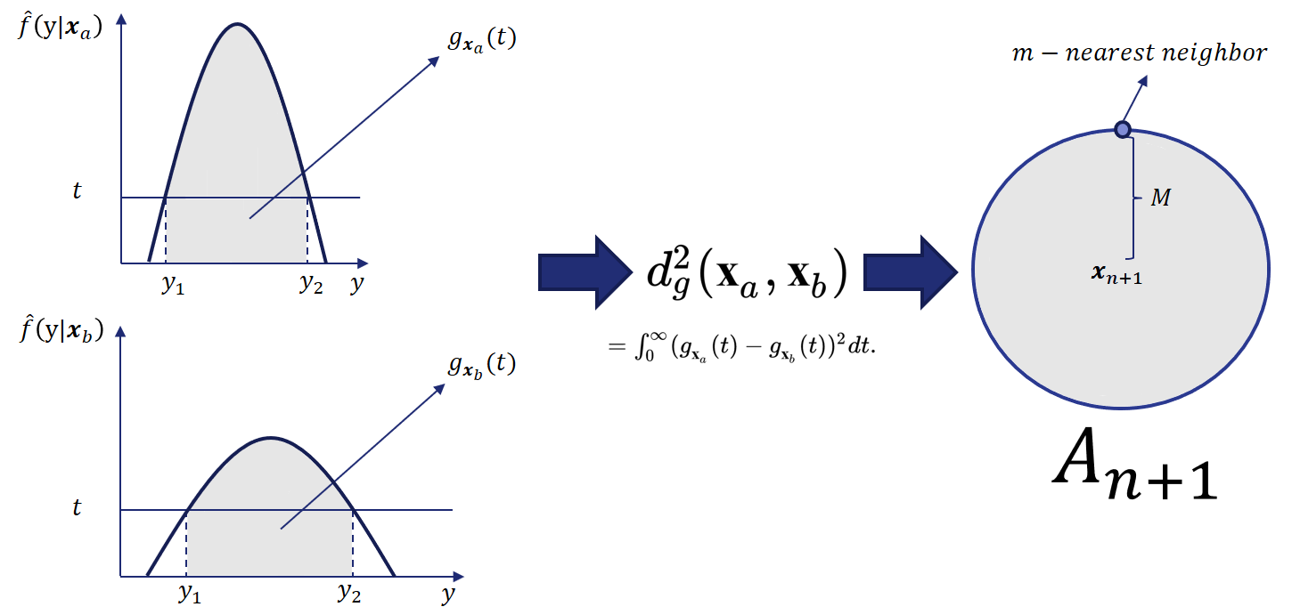
Figure 2: Illustration of the profile distance, which is used in CD-split for partitioning the feature space.

Definition 3.5 (Profile distance).

The profile distance between ${\mathbf{x}}_{a},{\mathbf{x}}_{b}\in\mathcal{X}$ is

$$d_{g}^{2}({\mathbf{x}}_{a},{\mathbf{x}}_{b}) :=\int_{0}^{\infty}\left(g_{{\mathbf{x}}_{a}}(t)-g_{{\mathbf{x}}_{b}}(t)\right)^{2}dt,$$

Contrary to the Euclidean distance, the profile distance is appropriate even for high-dimensional data. For instance, two points might be far in Euclidean distance and still have similar conditional densities. In this case one would like these points to be on the same partition element. The profile obtains this result by measuring the distance between instances based on the distance between their conditional densities. By grouping points with similar conditional densities, the profile distance allows partition elements to be larger without compromising too much the approximation of local validity to conditional validity. This property is illustrated in the following examples.

Example 3.6.

[Location family] Let $h(y)$ be a density, $\mu({\mathbf{x}})$ a function, and $Y|{\mathbf{x}}\sim h(y-\mu({\mathbf{x}}))$. In this case, $d_{g}({\mathbf{x}}_{a},{\mathbf{x}}_{b})=0$, for every ${\mathbf{x}}_{a},{\mathbf{x}}_{b}\in\mathbb{R}^{d}$. For instance, if $Y|{\mathbf{x}}\sim N(\beta^{t}{\mathbf{x}},\sigma^{2})$, then all instances have the same profile. Indeed, in this special scenario, if CD-split uses a unitary partition, then conditional validity is obtained.

Example 3.7.

[Irrelevant features] If ${\mathbf{x}}_{S}$ is a subset of the features such that $f(y|{\mathbf{x}})=f(y|{\mathbf{x}}_{S})$, then $d_{g}({\mathbf{x}}_{a},{\mathbf{x}}_{b})$ does not depend on the irrelevant features, $S^{c}$. While irrelevant features do not affect the profile distance, they can have a large impact in the Euclidean distance in high-dimensional settings.

Also, if all samples that fall into the same partition as ${\mathbf{x}}_{n+1}$ have the same profile as ${\mathbf{x}}_{n+1}$ according to $f$, then the statistics used in CD-split , $\mathcal{T}({\mathbf{x}}_{n+1},\mathbb{D})$ are i.i.d. data. Thus, the quantile used in CD-split will be the $\alpha$ quantile of $f(Y_{n+1}|{\mathbf{x}}_{n+1})$. This in turn makes $C({\mathbf{x}}_{n+1})$ the smallest prediction band with conditional validity of $1-\alpha$. Theorem 3.8, below, formalizes this statement.

Theorem 3.8.

Assume that all samples that fall into the same partition as ${\mathbf{x}}_{n+1}$, say $({\mathbf{X}}_{1},Y_{1}),\ldots,({\mathbf{X}}_{m},Y_{m})$, are such that $g_{{\mathbf{x}}_{i}}=g_{{\mathbf{x}}_{n+1}}$, and that ${\widehat{f}}(y|{\mathbf{x}})=f(y|{\mathbf{x}})$ is continuous as a function of $y$ for every ${\mathbf{x}}\in\mathcal{X}$. Let $T_{m}:=q(\alpha;\mathcal{T}({\mathbf{x}}_{n+1},\mathbb{D}))$ be the cutoff used in CD-split. Then, for every fixed $\alpha\in(0,1)$

$$T_{m}\xrightarrow[a.s.]{m\longrightarrow\infty}t^{*}$$

where $t^{*}=t^{*}({\mathbf{x}}_{n+1},\alpha)$ is the cutoff associated to the oracle band (i.e., the smallest predictive region with coverage $1-\alpha$).

Given the above reasons, the profile density captures what is needed of a meaningful neighborhood that contains many samples even in high dimensions. Indeed, consider a partition of the feature space, $\mathcal{A}$, that has the property that all samples that belong to the same element of $\mathcal{A}$ have the same oracle cutoff $t^{*}$. Theorem 3.9 shows that the coarsest partition that has this property is the one induced by the profile distance.

Theorem 3.9.

Assume that ${\widehat{f}}(y|{\mathbf{x}})=f(y|{\mathbf{x}})$ is continuous as a function of $y$ for every ${\mathbf{x}}\in\mathcal{X}$. For each sample ${\mathbf{x}}\in\mathcal{X}$ and miscoverage level $\alpha\in(0,1)$, let $t^{*}({\mathbf{x}},\alpha)$ be the cutoff of the oracle band for $f(y|{\mathbf{x}})$ with coverage $1-\alpha$. Consider the equivalence relation ${\mathbf{x}}_{a}\sim{\mathbf{x}}_{b}\iff d_{g}({\mathbf{x}}_{a},{\mathbf{x}}_{b})=0$. Then

1. if ${\mathbf{x}}_{a}\sim{\mathbf{x}}_{b}$, then $t^{*}({\mathbf{x}}_{a},\alpha)=t^{*}({\mathbf{x}}_{b},\alpha)$ for every $\alpha\in(0,1)$

2. if $\sim^{\prime}$ is any other equivalence relation such that ${\mathbf{x}}_{a}\sim^{\prime}{\mathbf{x}}_{b}$ implies that $t^{*}({\mathbf{x}}_{a},\alpha)=t^{*}({\mathbf{x}}_{b},\alpha)$ for every $\alpha\in(0,1)$, then ${\mathbf{x}}_{a}\sim^{\prime}{\mathbf{x}}_{b}\Rightarrow{\mathbf{x}}_{a}\sim{\mathbf{x}}_{b}$.

We therefore always use CD-split with the profile distance. In order to compute the prediction bands, we still need to define the centroids ${\mathbf{x}}_{i}^{c}$. Ideally, the partitions should be such that (i) all sample points inside a given element of the partition have similar profile, and (ii) sample points that belong to different elements of the partition have profiles that are very different from each other. We accomplish this by choosing the partitions by applying a k-means++ clustering algorithm (arthur2007k), but using the profile distance instead of the Euclidean one. This is done by applying the standard (Euclidean) k-means++ algorithm to the data points ${\mathbf{w}}_{i}:=\tilde{g}({\mathbf{x}}_{i})$, where $\tilde{g}({\mathbf{x}}_{i})$ is a discretization of the function $g({\mathbf{x}}_{i})$, obtained by evaluating $g({\mathbf{x}}_{i})$ on a grid of values. ${\mathbf{w}}_{1}^{c}$,…,${\mathbf{w}}_{J}^{c}$ are then the centroids of such clusters. Figure 3 illustrates the partitions that are obtained in one dataset. The profile distance allows samples that are far from each other in the Euclidean sense to fall into the same element of the partition. This is the key reason why our method scales to high-dimensional datasets.

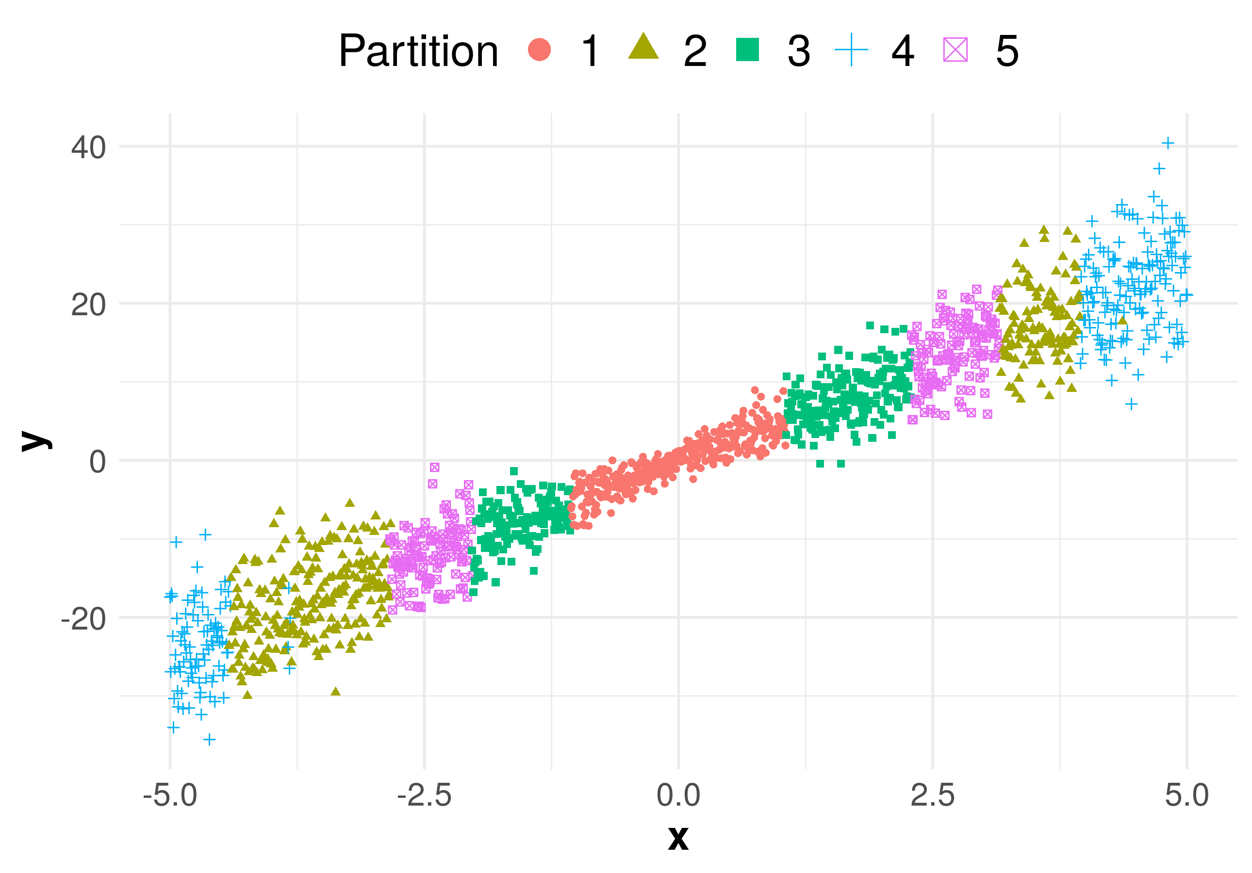
Figure 3: Scatter plot of data generated according to $Y|x\sim N(5x,1+|x|)$. Colors indicate partitions that were obtained using the profile of the estimated densities. Because points that are far from each other on the $x$-axis can belong to the same element of the partition, this approach to partition the feature space increases the number of data points that belong to each element. These elements however preserve the optimal cutoff (Theorem 3.9).

Algorithm 2 shows pseudo-code for implementing CD-split.

Algorithm 2 CD-split

Input: Data $({\mathbf{x}}_{i},Y_{i})$, $i=1,...,n$, miscoverage level $\alpha\in(0,1)$, algorithm $\mathcal{B}$ for fitting conditional density function, number of elements of the partition $J$.
Output: Prediction band for ${\mathbf{x}}_{n+1}\in\mathbb{R}^{d}$

1:  Randomly split $\{1,2,...,n\}$ into two subsets $\mathbb{D}$ and $\mathbb{D}^{\prime}$

2:  Fit $\hat{f}=\mathcal{B}(\{({\mathbf{x}}_{i},Y_{i}):i\in\mathbb{D}^{\prime}\})$  // Estimate cumulative density function

3:  Compute $\mathcal{A}$, the partition of $\mathcal{X}$, by applying k-means++ on the profiles of the samples in $\mathbb{D}$’

4:  Compute $g_{{\mathbf{x}}_{n+1}}(t)=\int_{\{y:\hat{f}(y|{\mathbf{x}})\geq t\}}\hat{f}(y|{\mathbf{x}})dy$, for all $t>0$  // Profile of the density (Definition 3.4)

5:  Find $A({\mathbf{x}}_{n+1})\in\mathcal{A}$, the element of $\mathcal{A}$ such that ${\mathbf{x}}_{n+1}\in\mathcal{A}$

6:  Compute $g_{{\mathbf{x}}_{i}}(t)=\int_{\{y:\hat{f}(y|{\mathbf{x}})\geq t\}}\hat{f}(y|{\mathbf{x}})dy$, for all $t>0$ and $i\in\mathbb{D}$  // Profile of the densities (Definition 3.4)

7:  Let $\mathcal{T}({\mathbf{x}}_{n+1},\mathbb{D})=\{\hat{f}(y_{i}|{\mathbf{x}}_{i}),i\in\mathbb{D}:{\mathbf{x}}_{i}\in A({\mathbf{x}}_{n+1})\}$

8:  Let $t=q(\alpha;\mathcal{T}({\mathbf{x}}_{n+1},\mathbb{D}))$  // Compute the $\alpha$- quantile of the set $\mathcal{T}({\mathbf{x}}_{n+1},\mathbb{D})$

9:  return $\left\{y:\hat{f}(y|{\mathbf{x}}^{*})\geq t\right\}$

3.1 Multiclass classification

If the sample space $\mathcal{Y}$ is discrete, we use a similar construction to that of Definition 3.1. More precisely, the CD-split prediction band is given by

$$C({\mathbf{x}}_{n+1})=\left\{y:\widehat{{\mathbb{P}}}(Y=y|{\mathbf{x}}_{n+1})\geq q(\alpha;\mathcal{T}({\mathbf{x}}_{n+1},\mathbb{D}))\right\},$$

where

$$\mathcal{T}({\mathbf{x}}_{n+1},\mathbb{D})=\left\{\widehat{{\mathbb{P}}}(Y_{i}=y_{i}|{\mathbf{x}}_{i}),i=1,\ldots,n:{\mathbf{x}}_{i}\in A({\mathbf{x}}_{n+1})\right\},$$

$A({\mathbf{x}}_{n+1})$ is the element of $\mathcal{A}$ to which ${\mathbf{x}}_{n+1}$ belongs to, and

$$d_{g}^{2}({\mathbf{x}}_{a},{\mathbf{x}}_{b})=\sum_{y\in\mathcal{Y}}\left(\widehat{{\mathbb{P}}}(Y=y|{\mathbf{x}}_{a})-\widehat{{\mathbb{P}}}(Y=y|{\mathbf{x}}_{b})\right)^{2}.$$

Theorems analogous to those presented in the last section hold in the classification setting as well.

Remark 2.

While CD-split is developed to control the coverage of $C$ conditional on the value ${\mathbf{x}}_{n+1}$, in a classification setting some methods (e.g. Sadinle et al., 2019) control class-specific coverage, defined as

$${\mathbb{P}}(Y_{n+1}\in C({\mathbf{X}}_{n+1})|Y_{n+1}=y)\geq 1-\alpha_{y}.$$

4 Experiments

We consider the following settings with $d=20$ covariates:

• [Asymmetric] ${\mathbf{X}}=(X_{1},\ldots,X_{d})$, with $X_{i}\overset{\text{iid}}{\sim}\mbox{Unif}(-5,5)$, and $Y|{\mathbf{x}}=5x_{1}+\epsilon$, where $\epsilon\sim\mbox{Gamma}(1+2|x_{1}|,1+2|x_{1}|)$

• [Bimodal] ${\mathbf{X}}=(X_{1},\ldots,X_{d})$, with $X_{i}\overset{\text{iid}}{\sim}\mbox{Unif}(-1.5,1.5)$, and $Y|{\mathbf{x}}\sim 0.5\mbox{N}(f({\mathbf{x}})-g({\mathbf{x}}),\sigma^{2}({\mathbf{x}}))+0.5\mbox{N}(f({\mathbf{x}})+g({\mathbf{x}}),\sigma^{2}({\mathbf{x}})),$ with $f({\mathbf{x}})=(x_{1}-1)^{2}(x_{1}+1),$ $g({\mathbf{x}})=2{\mathbb{I}}(x_{1}\geq-0.5)\sqrt{x_{1}+0.5}$, and $\sigma^{2}({\mathbf{x}})=1/4+|x_{1}|$. This is the example from (Lei and Wasserman,, 2014) with $d-1$ irrelevant variables added.

• [Heteroscedastic] ${\mathbf{X}}=(X_{1},\ldots,X_{d})$, with $X_{i}\overset{\text{iid}}{\sim}\mbox{Unif}(-5,5)$, and $Y|{\mathbf{x}}\sim\mbox{N}(x_{1},1+|x_{1}|)$

• [Homoscedastic] ${\mathbf{X}}=(X_{1},\ldots,X_{d})$, with $X_{i}\overset{\text{iid}}{\sim}\mbox{Unif}(-5,5)$, and $Y|{\mathbf{x}}\sim\mbox{N}(x_{1},1)$

We compare the performance of the following methods:

• [Reg-split] The regression-split method (Lei et al.,, 2018), based on the conformal score $|Y_{i}-\widehat{r}({\mathbf{x}}_{i})|$, where $\widehat{r}$ is an estimate of the regression function.

• [Local Reg-split] The local regression-split method (Lei et al.,, 2018), based on the conformal score $\frac{|Y_{i}-\widehat{r}({\mathbf{x}}_{i})|}{\widehat{\rho}({\mathbf{x}}_{i})}$, where $\widehat{\rho}({\mathbf{x}}_{i})$ is an estimate of the conditional mean absolute deviation of $|Y_{i}-r({\mathbf{x}}_{i})|{\mathbf{x}}_{i}$.

• [Quantile-split] The conformal quantile regression method (Romano et al.,, 2019; Sesia and Candès,, 2019), based on conformalized quantile regression.

• [Dist-split] From section 2.

• [CD-split] From section 3 with partitions of size $J=\lceil n/100\rceil$.

For each sample size, $n$, we use a coverage level of $1-\alpha=90\%$ and run each setting 5,000 times. In order to make fair comparisons between the various approaches, we use random forests (Breiman,, 2001) to estimate all quantities needed, namely: the regression function in Reg-split, the conditional mean absolute deviation in Local Reg-split, the conditional quantiles via quantile forests (Meinshausen,, 2006) in Quantile-split, and the conditional density via FlexCode (Izbicki and Lee,, 2017) in Dist-split and CD-split. A conditional cumulative distribution estimate, $\widehat{F}(y|{\mathbf{x}})$ is obtained by integrating the conditional density estimate: $\widehat{F}(y|{\mathbf{x}})=\int_{-\infty}^{y}\widehat{f}(y|{\mathbf{x}})dy$. The tuning parameters of all methods were set to be the default values of the packages that were used.

(a)

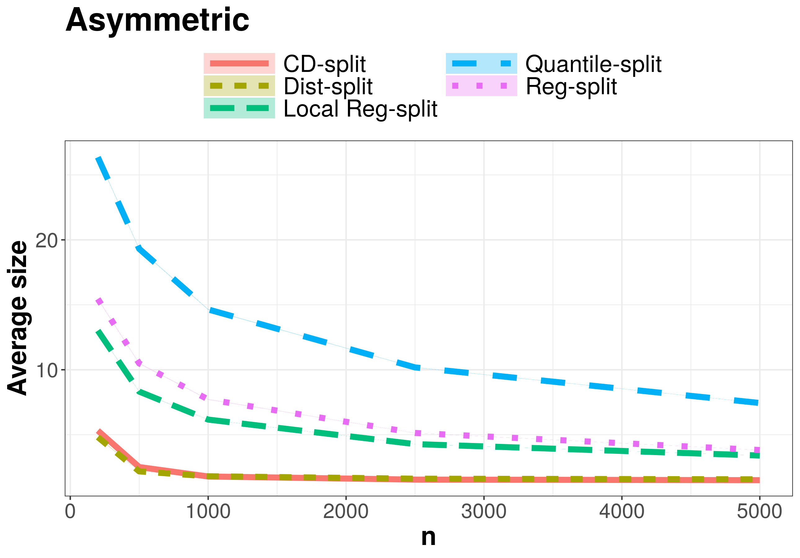
(b)

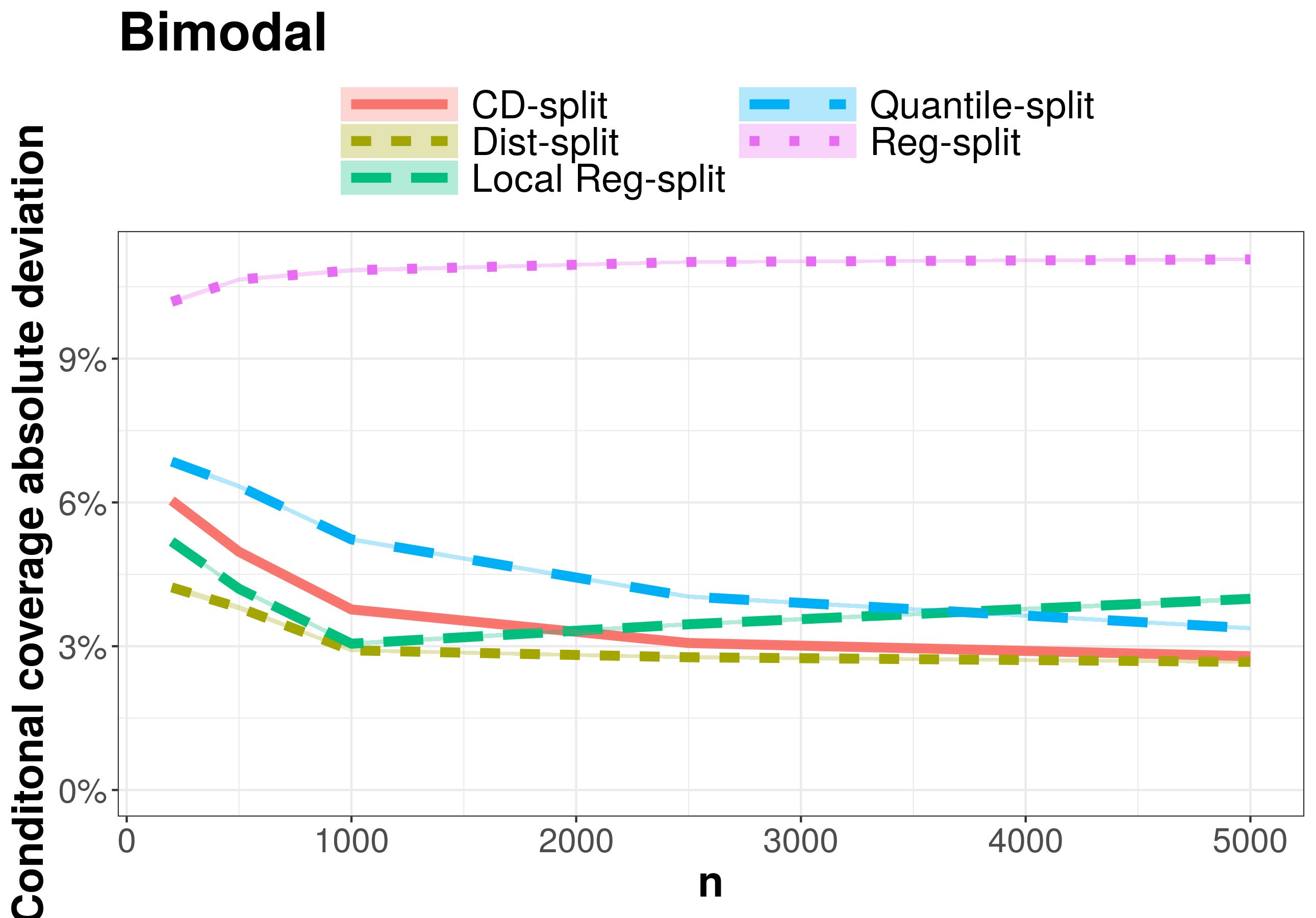
(c)

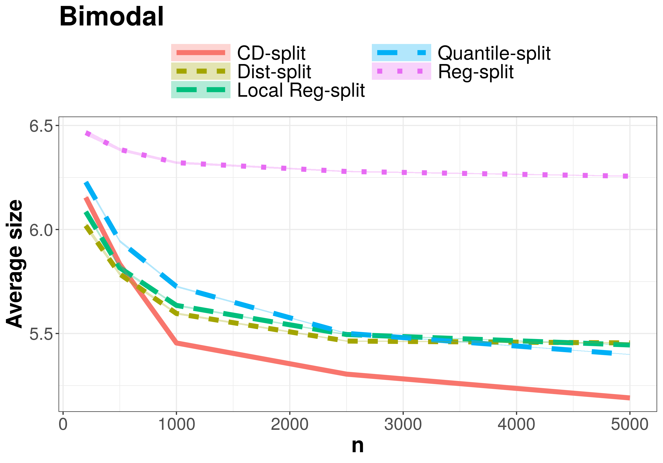
(d)

(e)

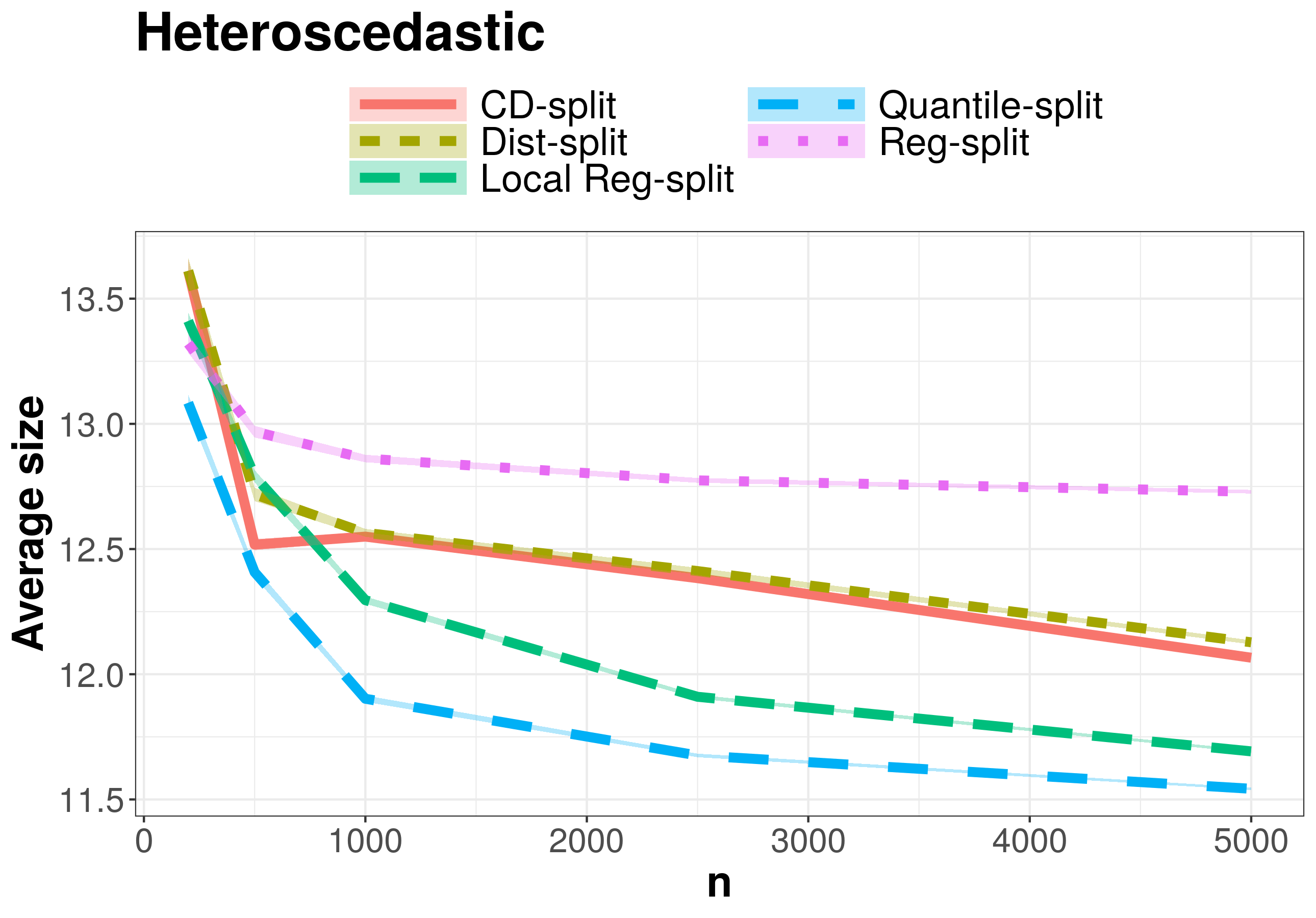
(f)

(g)

(h)

Figure 4: Performance of each regression method as a function of the sample size. Left panels show how much the conditional coverage vary with ${\mathbf{x}}$; right panels display the average size of the prediction bands.

Figure 4 shows the performance of each method as a function of the sample size. While the left side figures display how well each method controls conditional coverage, the right side displays the average size of the regions that are obtained. The control of the conditional coverage is measured through the conditional coverage absolute deviation, that is, ${\mathbb{E}}[|{\mathbb{P}}(Y^{*}\in C({\mathbf{X}}^{*})|{\mathbf{X}}^{*})-(1-\alpha)|]$. Since all of the methods obtain marginal coverage very close to the nominal $90\%$ level, this information is not displayed in the figure. Figure 4 shows that, in all settings, CD-split is the method which best controls conditional coverage. Also, in most cases its prediction bands also have the smallest size. Similarly, Dist-split frequently is the second method with both highest control of conditional coverage and also smallest prediction bands.

We also apply CD-split to a classification setting. We consider ${\mathbf{X}}=(X_{1},\ldots,X_{d})$, with $X_{i}\overset{\text{iid}}{\sim}N(0,1)$ and $Y|{\mathbf{X}}$ follows the logistic model, ${\mathbb{P}}(Y=i|{\mathbf{x}})\propto\exp\left\{\boldsymbol{\beta}\cdot{\mathbf{x}}\right\}$, where $\boldsymbol{\beta}=(-6,-5,-1.5,0,1.5,5,6)$. We compare CD-split to Probability-split, the method described in Sadinle et al., (2019, Sec. 4.3), which has the goal of controlling global coverage. Probability-split is a particular case of CD-split: it corresponds to applying CD-split with $J=1$ partitions. Figure 5 shows the results. CD-split better controls conditional coverage. On the other hand, its prediction bands are, on average, larger than those of Probability-split.

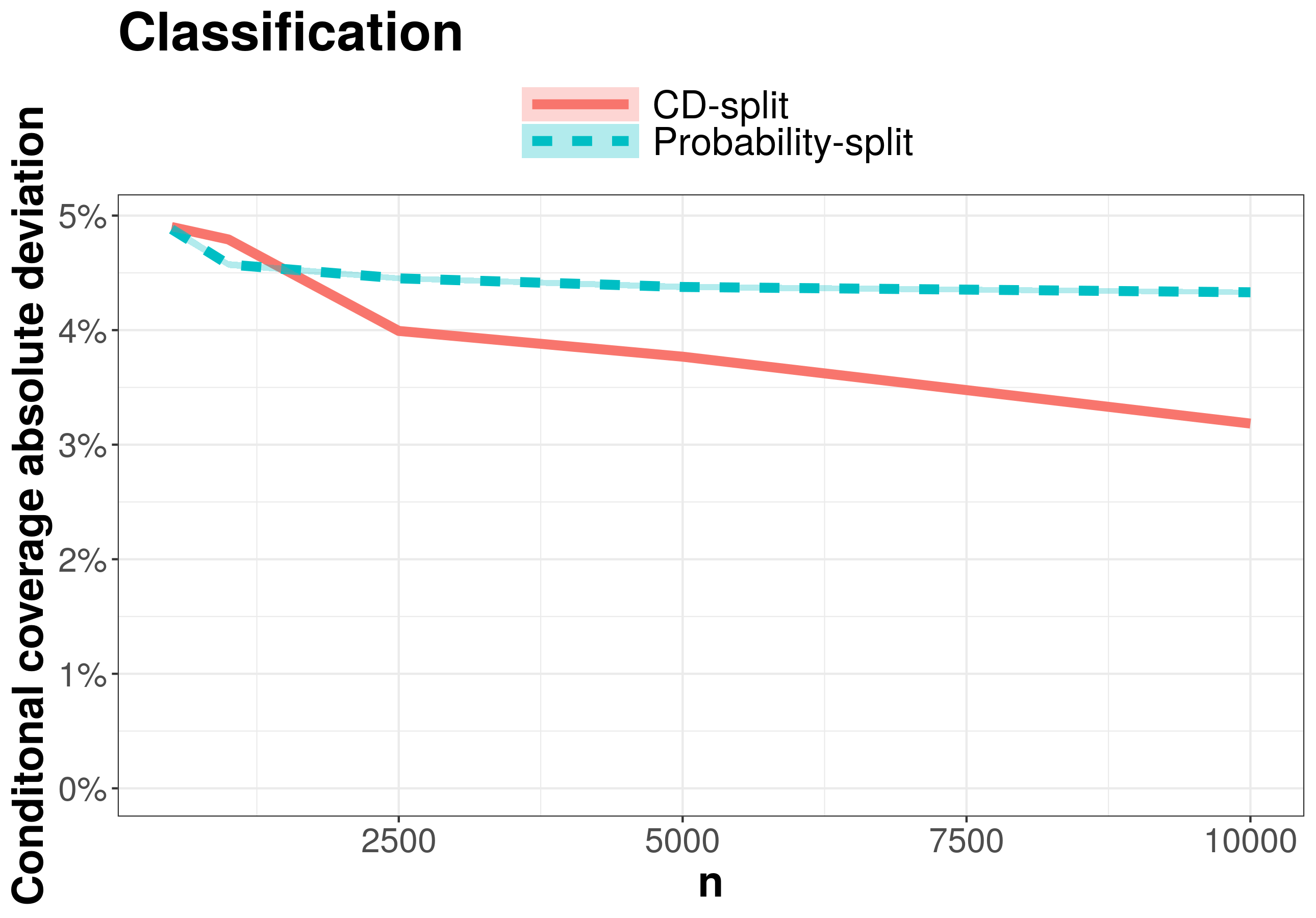
(a)

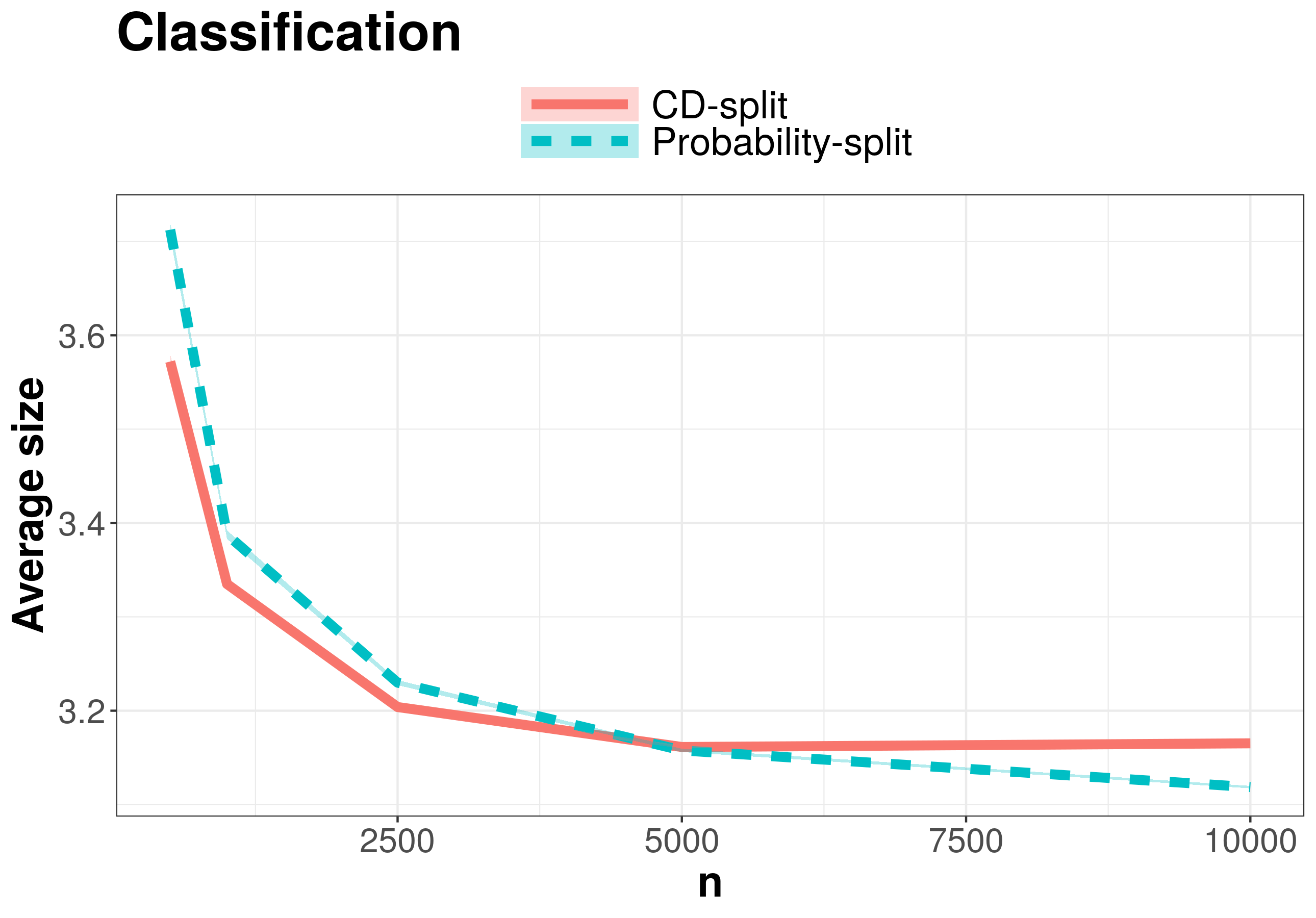
(b)

Figure 5: Performance of each classification method as a function of the sample size. Left panel shows how much the conditional coverage vary with ${\mathbf{x}}$; right panel displays the average size of the prediction bands.

5 Final remarks

We introduce Dist-split and CD-split, which obtain asymptotic conditional coverage and converge to optimal oracle bands, even in high-dimensional feature spaces. These results do not require assumptions about the dependence between the target variable and the features. Both methods are based on estimating conditional densities. While Dist-split necessarily leads to intervals, which are easier to interpret, CD-split leads to smaller prediction regions. A simulation study shows that both methods yield smaller prediction bands and better control of conditional coverage than other methods in the literature under a variety of settings. We also show that CD-split leads to good results in classification problems.

CD-split is based on a novel data-driven metric on the feature space that appropriate for defining neighborhoods for conformal methods, in particular in high-dimensional settings. It might be possible to use this metric with other conformal methods to obtain asymptotic conditional coverage.

R code for implementing Dist-split and CD-split is available on https://github.com/rizbicki/predictionBands.

Acknowledgements

This study was financed in part by the Coordenação de Aperfeiçoamento de Pessoal de Nível Superior - Brasil (CAPES) - Finance Code 001. Rafael Izbicki is grateful for the financial support of FAPESP (grants 2017/03363-8 and 2019/11321-9) and CNPq (grant 306943/2017-4). The authors are also grateful for the suggestions given by Luís Gustavo Esteves and Jing Lei.

Proofs

Definition 5.1.

$U_{\lfloor\alpha\rfloor}$ and $U_{\lceil\alpha\rceil}$ are the $\lfloor n^{-1}(n\alpha)\rfloor$ $\lceil n^{-1}(n\alpha)\rceil$ empirical quantiles of $U_{1},\ldots,U_{n}$,

Related to Dist-split

Proof of Theorem 2.2.

Let $U_{i}={\widehat{F}}(Y_{i}|{\mathbf{X}}_{i})$. Since $({\mathbf{X}}_{i},Y_{i})$ are i.i.d. continuous random variables and ${\widehat{F}}$ is continuous, obtain that $U_{i}$ are i.i.d. continuous random variables.

$$1-\alpha \leq{\mathbb{P}}\left(U_{n+1}\in[{U_{\lfloor 0.5\alpha\rfloor}};{U_{\lceil 1-0.5\alpha\rceil}}]\right)\leq 1-\alpha+(n+1)^{-1}.$$

The conclusion follows from noticing that

$${\mathbb{P}}\left(U_{n+1}\in[{U_{\lfloor 0.5\alpha\rfloor}};{U_{\lceil 1-0.5\alpha\rceil}}]\right)$$

$$= {\mathbb{P}}\left(Y_{n+1}\in[{\widehat{F}}^{-1}({U_{\lfloor 0.5\alpha\rfloor}}|{\mathbf{X}}_{n+1});{\widehat{F}}^{-1}({U_{\lceil 1-0.5\alpha\rceil}}|{\mathbf{X}}_{n+1})]\right)$$

$$= {\mathbb{P}}(Y_{n+1}\in C({\mathbf{X}}_{n+1}))$$

∎

Lemma 5.2.

Let $I_{1}=\left\{i\leq n:|{\widehat{F}}(Y_{i}|{\mathbf{X}}_{i})-F(Y_{i}|{\mathbf{X}}_{i})|<\eta_{n}^{1/3}\right\}$ and $I_{2}=\{1,\ldots,n\}-I_{1}$. Under Assumption 2.3, $|I_{2}|=o_{P}(n)$ and $|I_{1}|=n+o_{P}(n)$.

Proof.

Let $A_{n}=\left\{{\mathbb{E}}\left[\sup_{y\in{\mathcal{Y}}}\left({\widehat{F}}(y|{\mathbf{X}})-F(y|{\mathbf{X}})\right)^{2}\big{|}{\widehat{F}}\right]\geq\eta_{n}\right\}$ and $B_{n}=\left\{|{\widehat{F}}(Y|{\mathbf{X}})-F(Y|{\mathbf{X}})|\geq\eta_{n}^{1/3}\right\}$.

$${\mathbb{P}}(B_{n}) ={\mathbb{E}}[{\mathbb{P}}(B_{n}|{\widehat{F}}){\mathbb{I}}(A_{n})]+{\mathbb{E}}[{\mathbb{P}}(B_{n}|{\widehat{F}}){\mathbb{I}}(A_{n}^{c})]$$

$$\leq{\mathbb{P}}(A_{n})+{\mathbb{E}}\left[\frac{{\mathbb{E}}[({\widehat{F}}(Y|{\mathbf{X}})-F(Y|{\mathbf{X}}))^{2}|{\widehat{F}}]}{\eta_{n}^{2/3}}{\mathbb{I}}(A_{n}^{c})\right]$$

$$\leq\rho_{n}+\eta_{n}^{1/3}=o(1)$$

Note that $|I_{2}|\sim\text{Binomial}(n,{\mathbb{P}}(B_{n}))$. Since ${\mathbb{P}}(B_{n})=o(1)$, conclude that $|I_{2}|=o_{P}(n)$. That is, $|I_{1}|=n+o_{P}(n)$. ∎

Lemma 5.3.

Under Assumption 2.3, If $U_{i}={\widehat{F}}(Y_{i}|{\mathbf{X}}_{i})$, then for every $\alpha\in(0,1)$, $U_{\lfloor\alpha\rfloor}=\alpha+o_{P}(1)=U_{\lceil\alpha\rceil}$.

Proof.

Let $I_{1}$ and $I_{2}$ be such as in Lemma 5.2. Also, let $\hat{G}_{1}$, $G_{1}$ and $G_{0}$ be, the empirical quantiles of, respectively, $\{U_{i}:i\in I_{1}\}$, $\{F(Y_{i}|{\mathbf{X}}_{i}):i\in I_{1}\}$, and $\{F(Y_{i}|{\mathbf{X}}_{i}):i\leq n\}$. By definition of $I_{1}$, for every $\alpha^{*}\in[0,1]$, $\hat{G}_{1}^{-1}(\alpha^{*})=G_{1}^{-1}(\alpha^{*})+o(1)$. Also, $G_{0}^{-1}(\alpha^{*})=\alpha^{*}+o_{P}(1)$. Therefore, since

$$G_{0}^{-1}\left(\frac{|I_{1}|\alpha^{*}}{n}\right)\leq G_{1}^{-1}(\alpha^{*})\leq G_{0}^{-1}\left(\frac{|I_{1}|\alpha^{*}+|I_{2}|}{n}\right),$$

conclude that $\hat{G}_{1}^{-1}(\alpha^{*})=\alpha^{*}+o_{P}(1)$. Finally, since

$$\hat{G}^{-1}\left(\frac{n\alpha-|I_{2}|}{|I_{1}|}\right)\leq U_{\lfloor\alpha\rfloor}\leq U_{\lceil\alpha\rceil}\leq\hat{G}^{-1}\left(\frac{n\alpha}{|I_{1}|}\right),$$

Conclude that $U_{\lfloor\alpha\rfloor}=\alpha+o_{P}(1)=U_{\lceil\alpha\rceil}$. ∎

Lemma 5.4.

Let $U_{i}=\hat{F}(Y_{i}|{\mathbf{X}}_{i})$. Under Assumptions 2.3 and 2.4,

$${\widehat{F}}^{-1}(U_{[0.5\alpha]}|{\mathbf{X}}_{n+1}) =F^{-1}(0.5\alpha|{\mathbf{X}}_{n+1})+o_{P}(1)$$

$${\widehat{F}}^{-1}(U_{[1-0.5\alpha]}|{\mathbf{X}}_{n+1}) =F^{-1}(1-0.5\alpha|{\mathbf{X}}_{n+1})+o_{P}(1)$$

Proof.

In order to prove the first equality, it is enough to show that $F^{-1}(U_{[0.5\alpha]}|{\mathbf{X}}_{n+1})=F^{-1}(0.5\alpha|{\mathbf{X}}_{n+1})+o_{P}(1)$ and that ${\widehat{F}}^{-1}(U_{[0.5\alpha]}|{\mathbf{X}}_{n+1})=F^{-1}(U_{[0.5\alpha]}|{\mathbf{X}}_{n+1})+o_{P}(1)$. The first part follows from Lemma 5.3 and the continuity of $F(y|{\mathbf{x}})$ (Assumption 2.4). For the second part, note that, if $\sup_{y}|\hat{F}(y|{\mathbf{x}})-F(y|{\mathbf{x}})|<\eta_{n}$, then, for every $\alpha^{*}$, $|\hat{F}^{-1}(\alpha^{*})-F^{-1}(\alpha^{*})|\leq\eta_{n}\left(\inf_{y}\frac{dF(y|{\mathbf{x}})}{dy}\right)^{-1}$. Using this observation, the proof of the second part follows from Assumption 2.4, and observing that $U_{[0.5\alpha]}=0.5\alpha+o_{P}(1)$ (Lemma 5.3) and ${\mathbb{P}}(\sup_{y}|\hat{F}(y|{\mathbf{x}})-F(y|{\mathbf{x}})|\geq\eta_{n})=o(1)$ (Assumption 2.3).

The proof for the $1-.5\alpha$ quantile is analogous to the one for the $.5\alpha$ quantile. ∎

Proof of Theorem 2.5.

Follows directly from Lemma 5.4. ∎

Related to CD-split

Proof Theorem 3.3.

Let$\{i_{1},\ldots,i_{n_{j}}\}=\{i:{\mathbf{X}}_{i}\in A({\mathbf{x}}_{n+1})\}$, $U_{l}={\widehat{f}}(Y_{i_{l}}|{\mathbf{X}}_{i_{l}})$, for $l=1,\ldots,n_{j}$, and $U_{n_{j}+1}={\widehat{f}}(Y_{n+1}|{\mathbf{X}}_{n+1})$. Since $({\mathbf{X}}_{1},Y_{1}),\ldots,({\mathbf{X}}_{n_{j}},Y_{n_{j}}),({\mathbf{X}}_{n+1},Y_{n+1})$ are i.i.d. random variables, obtain that $U_{i}$ are i.i.d. random variables conditional on the event ${\mathbf{X}}_{n+1}\in A({\mathbf{x}}_{n+1})$ and on $i_{1},\ldots,i_{n_{j}}$. Therefore,

$$1-\alpha \leq{\mathbb{P}}\left(U_{m+1}\geq U_{[\alpha]}|{\mathbf{X}}_{n+1}\in A({\mathbf{x}}_{n+1}),i_{1},\ldots,i_{n_{j}}\right)$$

The conclusion follows from the fact that $Y_{n+1}\in C({\mathbf{X}}_{n+1})\iff U_{m+1}\geq U_{[1-\alpha]}$ and because this holds for every sequence $i_{1},\ldots,i_{n_{j}}$. ∎

Proof of Theorem 3.8.

Let $U_{i}:=f(Y_{i}|{\mathbf{x}}_{i})$, $i=1,\ldots,m$, $U_{n+1}:=f(Y_{n+1}|{\mathbf{x}}_{n+1})$, and $W:=({\mathbf{x}}_{1},\ldots,{\mathbf{x}}_{m},{\mathbf{x}}_{n+1})$. If $g_{{\mathbf{x}}_{i}}=g_{{\mathbf{x}}_{n+1}}$ for every $i=1,\ldots,m$, then $U_{1},\ldots,U_{m},U_{n+1}$ are i.i.d. conditional on $W$. Indeed, for every $t\in\mathbb{R}$,

$${\mathbb{P}}(U_{i}\geq t|W) ={\mathbb{P}}(f(Y_{i}|{\mathbf{x}}_{i})\geq t|{\mathbf{x}}_{i})$$

$$={\mathbb{P}}(f(Y_{n+1}|{\mathbf{x}}_{n+1})\geq t|{\mathbf{x}}_{n+1})$$

$$={\mathbb{P}}(U_{n+1}\geq t|{\mathbf{x}}_{n+1}),$$

where the next-to-last equality follows from the definition of the profile of the density.

For every $K\in\mathbb{R}$, let $Q(K):=\left|\{i:f(Y_{i}|{\mathbf{x}}_{i})\geq K\}\right|$. Because $U_{i}$’s are conditionally independent and identically distributed, then $Q(K)|W\sim\mbox{Binomial}(m,{\mathbb{P}}(f(Y_{1}|{\mathbf{x}}_{1})\geq K))$. It follows that $Q(K)/m\xrightarrow[a.s.]{m\longrightarrow\infty}{\mathbb{P}}(f(Y_{1}|{\mathbf{x}}_{1})\geq K)$. In particular, $Q(t^{*})/m\xrightarrow[a.s.]{m\longrightarrow\infty}1-\alpha$. Now, by definition $Q(T_{m})/m\xrightarrow[a.s.]{m\longrightarrow\infty}1-\alpha$. Conclude that $T_{m}\xrightarrow[a.s.]{m\longrightarrow\infty}t^{*}$.

∎

Proof of Theorem 3.9.

Item (i) was already shown as part of the proof of Theorem 3.8. To show (ii), assume that $t^{*}({\mathbf{x}}_{a},\alpha)=t^{*}({\mathbf{x}}_{b},\alpha)$ for every $\alpha\in(0,1)$. Now, notice that $t^{*}({\mathbf{x}}_{a},\alpha)$ is such that $g_{{\mathbf{x}}_{a}}(t^{*}({\mathbf{x}}_{a},\alpha))=1-\alpha.$ Conclude that $g_{{\mathbf{x}}_{a}}(t^{*}({\mathbf{x}}_{a},\alpha))=g_{{\mathbf{x}}_{b}}(t^{*}({\mathbf{x}}_{b},\alpha))$ for every $\alpha\in(0,1)$. Now, because ${\widehat{f}}$ is continuous, $\{t^{*}({\mathbf{x}}_{a},\alpha):\alpha\in(0,1)\}=\mbox{Im}({\widehat{f}}(\cdot|{\mathbf{x}}_{a}))$. Thus, $g_{{\mathbf{x}}_{a}}=g_{{\mathbf{x}}_{b}}$, and therefore ${\mathbf{x}}_{a}\sim{\mathbf{x}}_{b}$. ∎

References

• Barber et al., (2019) Barber, R. F., Candès, E. J., Ramdas, A., and Tibshirani, R. J. (2019). The limits of distribution-free conditional predictive inference. arXiv preprint arXiv:1903.04684.
• Breiman, (2001) Breiman, L. (2001). Random forests. Machine learning, 45(1):5–32.
• Guan, (2019) Guan, L. (2019). Conformal prediction with localization. arXiv preprint arXiv:1908.08558.
• Izbicki and Lee, (2017) Izbicki, R. and Lee, A. B. (2017). Converting high-dimensional regression to high-dimensional conditional density estimation. Electronic Journal of Statistics, 11(2):2800–2831.
• Lei et al., (2018) Lei, J., G’Sell, M., Rinaldo, A., Tibshirani, R. J., and Wasserman, L. (2018). Distribution-free predictive inference for regression. Journal of the American Statistical Association, 113(523):1094–1111.
• Lei and Wasserman, (2014) Lei, J. and Wasserman, L. (2014). Distribution-free prediction bands for non-parametric regression. Journal of the Royal Statistical Society: Series B (Statistical Methodology), 76(1):71–96.
• Lueckmann et al., (2017) Lueckmann, J.-M., Goncalves, P. J., Bassetto, G., Öcal, K., Nonnenmacher, M., and Macke, J. H. (2017). Flexible statistical inference for mechanistic models of neural dynamics. In Advances in Neural Information Processing Systems, pages 1289–1299.
• Meinshausen, (2006) Meinshausen, N. (2006). Quantile regression forests. Journal of Machine Learning Research, 7(Jun):983–999.
• Neter et al., (1996) Neter, J., Kutner, M. H., Nachtsheim, C. J., and Wasserman, W. (1996). Applied linear statistical models, volume 4. Irwin Chicago.
• Papadopoulos, (2008) Papadopoulos, H. (2008). Inductive conformal prediction: Theory and application to neural networks. In Tools in artificial intelligence. IntechOpen.
• Papamakarios et al., (2017) Papamakarios, G., Pavlakou, T., and Murray, I. (2017). Masked autoregressive flow for density estimation. In Advances in Neural Information Processing Systems, pages 2338–2347.
• Parmigiani and Inoue, (2009) Parmigiani, G. and Inoue, L. (2009). Decision theory: Principles and approaches, volume 812. John Wiley & Sons.
• Romano et al., (2019) Romano, Y., Patterson, E., and Candès, E. J. (2019). Conformalized quantile regression.
• Sadinle et al., (2019) Sadinle, M., Lei, J., and Wasserman, L. (2019). Least ambiguous set-valued classifiers with bounded error levels. Journal of the American Statistical Association, 114(525):223–234.
• Sesia and Candès, (2019) Sesia, M. and Candès, E. J. (2019). A comparison of some conformal quantile regression methods. arXiv preprint arXiv:1909.05433.
• Vovk, (2012) Vovk, V. (2012). Conditional validity of inductive conformal predictors. In Asian conference on machine learning, pages 475–490.
• Vovk et al., (2005) Vovk, V. et al. (2005). Algorithmic learning in a random world. Springer Science & Business Media.
• Vovk et al., (2009) Vovk, V., Nouretdinov, I., Gammerman, A., et al. (2009). On-line predictive linear regression. The Annals of Statistics, 37(3):1566–1590.