Dual-path RNN: efficient long sequence modeling for
time-domain single-channel speech separation

Abstract

Recent studies in deep learning-based speech separation have proven the superiority of time-domain approaches to conventional time-frequency-based methods. Unlike the time-frequency domain approaches, the time-domain separation systems often receive input sequences consisting of a huge number of time steps, which introduces challenges for modeling extremely long sequences. Conventional recurrent neural networks (RNNs) are not effective for modeling such long sequences due to optimization difficulties, while one-dimensional convolutional neural networks (1-D CNNs) cannot perform utterance-level sequence modeling when its receptive field is smaller than the sequence length. In this paper, we propose dual-path recurrent neural network (DPRNN), a simple yet effective method for organizing RNN layers in a deep structure to model extremely long sequences. DPRNN splits the long sequential input into smaller chunks and applies intra- and inter-chunk operations iteratively, where the input length can be made proportional to the square root of the original sequence length in each operation. Experiments show that by replacing 1-D CNN with DPRNN and apply sample-level modeling in the time-domain audio separation network (TasNet), a new state-of-the-art performance on WSJ0-2mix is achieved with a 20 times smaller model than the previous best system.

Index Terms—  Speech separation, deep learning, time domain, recurrent neural networks

1 Introduction

Recent progress in deep learning-based speech separation has ignited the interest of the research community in time-domain approaches [1, 2, 3, 4, 5, 6]. Compared with standard time-frequency domain methods, time-domain methods are designed to jointly model the magnitude and phase information and allow direct optimization with respect to both time- and frequency-domain differentiable criteria [7, 8, 9].

Current time-domain separation systems can be mainly categorized into adaptive front-end and direct regression approaches. The adaptive front-end approaches aim at replacing the short-time Fourier transform (STFT) with a differentiable transform to build a front-end that can be learned jointly with the separation network. Separation is applied to the front-end output as with the conventional time-frequency domain methods applying the separation processes to spectrogram inputs [3, 4, 5]. Being independent of the traditional time-frequency analysis paradigm, these systems are able to have a much more flexible choice on the window size and the number of basis functions for the front-end. On the other hand, the direct regression approaches learn a regression function from an input mixture to the underlying clean signals without an explicit front-end, typically by using some form of one-dimensional convolutional neural networks (1-D CNNs) [2, 10, 7].

A commonality between the two categories is that they both rely on effective modeling of extremely long input sequences. The direct regression methods perform separation at the waveform sample level, while the number of the samples can usually be tens of thousands, or sometimes even more. The performance of the adaptive front-end methods also depend on selection of the window size, where a smaller window improves the separation performance at the cost of a significantly longer front-end representation [4, 11]. This poses an additional challenge as conventional sequential modeling networks, including RNNs and 1-D CNNs, have difficulty on learning such long-term temporal dependency [12]. Moreover, unlike RNNs that have dynamic receptive fields, 1-D CNNs with fixed receptive fields that are smaller than the sequence length are not able to fully utilize the sequence-level dependency [13].

In this paper, we propose a simple network architecture, which we refer to as dual-path RNN (DPRNN), that organizes any kinds of RNN layers to model long sequential inputs in a very simple way. The intuition is to split the input sequence into shorter chunks and interleave two RNNs, an intra-chunk RNN and an inter-chunk RNN, for local and global modeling, respectively. In a DPRNN block, the intra-chunk RNN first processes the local chunks independently, and then the inter-chunk RNN aggregates the information from all the chunks to perform utterance-level processing. For a sequential input of length $L$, DPRNN with chunk size $K$ and chunk hop size $P$ contains $S$ chunks, where $K$ and $S$ corresponds to the input lengths for the inter- and intra-chunk RNNs, respectively. When $K\approx S$, the two RNNs have a sublinear input length ($O(\sqrt{L})$) as opposed to the original input length ($O(L)$), which greatly decreases the optimization difficulty that arises when $L$ is extremely large.

Compared with other approaches for arranging local and global RNN layers, or more general the hierarchical RNNs that perform sequence modeling in multiple time scales [14, 15, 16, 17, 18, 19], the stacked DPRNN blocks iteratively and alternately perform the intra- and inter-chunk operations, which can be treated as an interleaved processing between local and global inputs. Moreover, the first RNN layer in most hierarchical RNNs still receives the entire input sequence, while in stacked DPRNN each intra- or inter-chunk RNN receives the same sublinear input size across all blocks. Compared with CNN-based architectures such as temporal convolutional networks (TCNs) that only perform local modeling due to the fixed receptive fields [4, 5, 20], DPRNN is able to fully utilize global information via the inter-chunk RNNs and achieve superior performance with an even smaller model size. In Section 4 we will show that by simply replacing TCN by DPRNN in a previously proposed time-domain separation system [4], the model is able to achieve a 0.7 dB (4.6%) relative improvement with respect to scale-invariant signal-to-noise ratio (SI-SNR) [8] on WSJ0-2mix with a 49% smaller model size. By performing the separation at the waveform sample level, i.e. with window size of 2 samples and hop size of 1 sample, a new state-of-the-art performance is achieved with a 20 times smaller model than the previous best system.

2 Dual-path Recurrent Neural Network

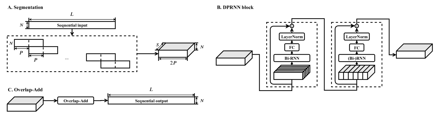
Fig. 1: System flowchart of dual-path RNN (DPRNN). (A) The segmentation stage splits a sequential input into chunks with or without overlaps and concatenates them to form a 3-D tensor. In our implementation, the overlap ratio is set to 50%. (B) Each DPRNN block consists of two RNNs that have recurrent connections in different dimensions. The intra-chunk bi-directional RNN is first applied to individual chunks in parallel to process local information. The inter-chunk RNN is then applied across the chunks to capture global dependency. Multiple blocks can be stacked to increase the total depth of the network. (C) The 3-D output of the last DPRNN block is converted back to a sequential output by performing overlap-add on the chunks.

2.1 Model design

A dual-path RNN (DPRNN) consists of three stages: segmentation, block processing, and overlap-add. The segmentation stage splits a sequential input into overlapped chunks and concatenates all the chunks into a 3-D tensor. The tensor is then passed to stacked DPRNN blocks to iteratively apply local (intra-chunk) and global (inter-chunk) modeling in an alternate fashion. The output from the last layer is transformed back to a sequential output with overlap-add method. Figure 1 shows the flowchart of the model.

2.1.1 Segmentation

For a sequential input $\bm{\mathrm{W}}\in\mathbb{R}^{N\times L}$ where $N$ is the feature dimension and $L$ is the number of time steps, the segmentation stage splits $\bm{\mathrm{W}}$ into chunks of length $K$ and hop size $P$. The first and last chunks are zero-padded so that every sample in $\bm{\mathrm{W}}$ appears and only appears in $K/P$ chunks, generating $S$ equal size chunks $\bm{\mathrm{D}}_{s}\in\mathbb{R}^{N\times K},\,s=1,\ldots,S$. All chunks are then concatenated together to form a 3-D tensor $\bm{\mathrm{T}}=[\bm{\mathrm{D}}_{1},\ldots,\bm{\mathrm{D}}_{S}]\in\mathbb{R}^{N\times K\times S}$.

2.1.2 Block processing

The segmentation output $\bm{\mathrm{T}}$ is then passed to the stack of $B$ DPRNN blocks. Each block transforms an input 3-D tensor into another tensor with the same shape. We denote the input tensor for block $b=1,\ldots,B$ as $\bm{\mathrm{T}}_{b}\in\mathbb{R}^{N\times K\times S}$, where $\bm{\mathrm{T}}_{1}=\bm{\mathrm{T}}$. Each block contains two sub-modules corresponding to intra- and inter-chunk processing, respectively. The intra-chunk RNN is always bi-directional and is applied to the second dimension of $\bm{\mathrm{T}}_{b}$, i.e., within each of the $S$ blocks:

$$\bm{\mathrm{U}}_{b}=[f_{b}(\bm{\mathrm{T}}_{b}[:,:,i]),\,i=1,\ldots,S]$$ (1)

where $\bm{\mathrm{U}}_{b}\in\mathbb{R}^{H\times K\times S}$ is the output of the RNN, $f_{b}(\cdot)$ is the mapping function defined by the RNN, and $\bm{\mathrm{T}}_{b}[:,:,i]\in\mathbb{R}^{N\times K}$ is the sequence defined by chunk $i$. A linear fully-connected (FC) layer is then applied to transform the feature dimension of $\bm{\mathrm{U}}_{b}$ back to that of $\bm{\mathrm{T}}_{b}$

$$\hat{\bm{\mathrm{U}}}_{b}=[\bm{\mathrm{G}}\bm{\mathrm{U}}_{b}[:,:,i]+\bm{\mathrm{m}},\,i=1,\ldots,S]$$ (2)

where $\hat{\bm{\mathrm{U}}}\in\mathbb{R}^{N\times K\times S}$ is the transformed feature, $\bm{\mathrm{G}}\in\mathbb{R}^{N\times H}$ and $\bm{\mathrm{m}}\in\mathbb{R}^{N\times 1}$ are the weight and bias of the FC layer, respectively, and $\bm{\mathrm{U}}_{b}[:,:,i]\in\mathbb{R}^{H\times K}$ represents chunk $i$ in $\bm{\mathrm{U}}_{b}$. Layer normalization (LN) [21] is then applied to $\hat{\bm{\mathrm{U}}}$, which we empirically found to be important for the model to have a good generalization ability:

$$LN(\hat{\bm{\mathrm{U}}}_{b}) =\frac{\hat{\bm{\mathrm{U}}}_{b}-\mu(\hat{\bm{\mathrm{U}}}_{b})}{\sqrt{\sigma(\hat{\bm{\mathrm{U}}}_{b})+\epsilon}}\odot\bm{\mathrm{z}}+\bm{\mathrm{r}}$$ (3)

where $\bm{\mathrm{z}},\bm{\mathrm{r}}\in\mathbb{R}^{N\times 1}$ are the rescaling factors, $\epsilon$ is a small positive number for numerical stability, and $\odot$ denotes the Hadamard product. $\mu(\cdot)$ and $\sigma(\cdot)$ are the mean and variance of the 3-D tensor defined as

$$\mu(\hat{\bm{\mathrm{U}}}_{b}) =\frac{1}{NKS}\sum_{i=1}^{N}\sum_{j=1}^{K}\sum_{s=1}^{S}\hat{\bm{\mathrm{U}}}_{b}[i,j,s]$$ (5)

$$\sigma(\hat{\bm{\mathrm{U}}}_{b}) =\frac{1}{NKS}\sum_{i=1}^{N}\sum_{j=1}^{K}\sum_{s=1}^{S}(\hat{\bm{\mathrm{U}}}_{b}[i,j,s]-\mu(\hat{\bm{\mathrm{U}}}_{b}))^{2}$$ (6)

A residual connection is then added between the output of LN operation and the input $\bm{\mathrm{T}}_{b}$:

$$\hat{\bm{\mathrm{T}}}_{b}=\bm{\mathrm{T}}_{b}+LN(\hat{\bm{\mathrm{U}}}_{b})$$ (7)

$\hat{\bm{\mathrm{T}}}_{b}$ is then served as the input to the inter-chunk RNN sub-module, where the RNN is applied to the last dimension, i.e. the aligned $K$ time steps in each of the $S$ blocks:

$$\bm{\mathrm{V}}_{b}=[h_{b}(\hat{\bm{\mathrm{T}}}_{b}[:,i,:]),\,i=1,\ldots,K]$$ (8)

where $\bm{\mathrm{V}}_{b}\in\mathbb{R}^{H\times K\times S}$ is the output of RNN, $h_{b}(\cdot)$ is the mapping function defined by the RNN, and $\hat{\bm{\mathrm{T}}}_{b}[:,i,:]\in\mathbb{R}^{N\times S}$ is the sequence defined by the $i$-th time step in all $S$ chunks. As the intra-chunk RNN is bi-directional, each time step in $\hat{\bm{\mathrm{T}}}_{b}$ contains the entire information of the chunk it belongs to, which allows the inter-chunk RNN to perform fully sequence-level modeling. As with the intra-chunk RNN, a linear FC layer and the LN operation are applied on top of $\bm{\mathrm{V}}_{b}$. A residual connection is also added between the output and $\hat{\bm{\mathrm{T}}}_{b}$ to form the output for DPRNN block $b$. For $b<B$, the output is served as the input to the next block $\bm{\mathrm{T}}_{b+1}$.

2.1.3 Overlap-Add

Denote the output of the last DPRNN block as $\bm{\mathrm{T}}_{B+1}\in\mathbb{R}^{N\times K\times S}$. To transform it back to a sequence, the overlap-add method is applied to the $S$ chunks to form output $\bm{\mathrm{Q}}\in\mathbb{R}^{N\times L}$.

2.2 Discussion

Consider the sum of the input sequence lengths for the intra- and inter-chunk RNNs in a single block denoted by $K+S$ where the hop size is set to be 50% (i.e. $P=K/2$) as in Figure 1. It is simple to see that $S=\lceil 2L/K\rceil+1$ where $\lceil\cdot\rceil$ is the ceiling function. To achieve minimum total input length $K+S=K+\lceil 2L/K\rceil+1$, $K$ should be selected such that $K\approx\sqrt{2L}$, and then $S$ also satisfies $S\approx\sqrt{2L}\approx K$. This gives us sublinear input length ($O(\sqrt{L})$) rather than the original linear input length ($O(L)$).

For tasks that require online processing, the inter-chunk RNN can be made uni-directional, scanning from the first up to the current chunks. The later chunks can still utilize the information from all previous chunks, and the minimal system latency is thus defined by the chunk size $K$. This is unlike standard CNN-based models that can only perform local processing due to the fixed receptive field or conventional RNN-based models that perform frame-level instead of chunk-level modeling. The performance difference between the online and offline settings, however, is beyond the scope of this paper.

3 Experimental procedures

3.1 Model configurations

Although DPRNN can be applied to any systems that require long-term sequential modeling, we investigate its application to the time-domain audio separation network (TasNet) [1, 22, 4], an adaptive front-end method that achieves high speech separation performance on a benchmarking dataset. TasNet contains three parts: (1) a linear 1-D convolutional encoder that encapsulates the input mixture waveform into an adaptive 2-D front-end representation, (2) a separator that estimates $C$ masking matrices for $C$ target sources, and (3) a linear 1-D transposed convolutional decoder that converts the masked 2-D representations back to waveforms. We use the same encoder and decoder design as in [4] while the number of filters is set to be 64. As for the separator, we compare the proposed deep DPRNN with the optimally configured TCN described in [4]. We use 6 DPRNN blocks using BLSTM [23] as the intra- and inter-chunk RNNs with 128 hidden units in each direction. The chunk size $K$ for DPRNN is defined empirically according to the length of the front-end representation such that $K\approx\sqrt{2L}$ in the training set as discussed in Section 2.2.

3.2 Dataset

We evaluate our approach on two-speaker speech separation and recognition tasks. The separation-only experiment is conducted on the widely-used WSJ0-2mix dataset [24]. WSJ0-2mix contains 30 hours of 8k Hz training data that are generated from the Wall Street Journal (WSJ0) si_tr_s set. It also has 10 hours of validation data and 5 hours of test data generated by using the si_dt_05 and si_et_05 sets, respectively. Each mixture is artificially generated by randomly selecting different speakers from the corresponding set and mixing them at a random relative signal-to-noise ratio (SNR) between -5 and 5 dB. For the speech separation and recognition experiment, we create 200 hours and 10 hours of artificially mixed noisy reverberant mixtures sampled from the Librispeech dataset [25] for training and validation, respectively. The 16 kHz signals are convolved with room impulse responses generated by the image method [26]. The length and width of the room are randomly sampled between 2 and 10 meters, and the height is randomly sampled between 2 and 5 meters. The reverberation time (T60) is randomly sampled between 0.1 and 0.5 seconds. The locations for the speakers as well as the single microphone are all randomly sampled. The two reverberated signals are rescaled to a random SNR between -5 and 5 dB, and further shifted such that the overlap ratio between the two speakers is 50% on average. The resultant mixture is further corrupted by random isotropic noise at a random SNR between 10 and 20 dB [27]. For evaluation, we generate mixture in the same manner sampled from Microsoft’s internal gender-balanced clean speech collection consisting of 44 speakers. The target for separation is the reverberant clean speech for both speakers.

3.3 Experiment configurations

We train all models for 100 epochs on 4-second long segments. The learning rate is initialized to $1e^{-3}$ and decays by 0.98 for every two epochs. Early stopping is applied if no best model is found in the validation set for 10 consecutive epochs. Adam [28] is used as the optimizer. Gradient clipping with maximum $L_{2}$-norm of 5 is applied for all experiments. All models are trained with utterance-level permutation invariant training (uPIT) [29] to maximize scale-invariant SNR (SI-SNR) [8].

The effectiveness of the systems is assessed both in terms of signal fidelity and speech recognition accuracy. The degree of improvement in the signal fidelity is measured by signal-to-distortion ratio improvement (SDRi) [30] as well as SI-SNR improvement (SI-SNRi). The speech recognition accuracy is measured by the word error rate (WER) on both separated speakers.

4 Results and discussions

4.1 Results on WSJ0-2mix

We first report the results on the WSJ0-2mix dataset. Table 1 compares the TasNet-based systems with different separator networks. We can see that simply replacing TCN by DPRNN improves the separation performance by 4.6% with a 49% smaller model. This shows the superiority of the proposed local-global modeling to the previous CNN-based local-only modeling. Moreover, the performance can be consistently improved by further decreasing the filter length (and the hop size as a consequence) in the encoder and decoder. The best performance is obtained when the filter length is 2 samples with an encoder output of more than 30000 frames. This can be extremely hard or even impossible for standard RNNs or CNNs to model, while with the proposed DPRNN the use of such a short filter becomes possible and achieves the best performance.

Table 2 compares the DPRNN-TasNet with other previous systems on WSJ0-2mix. We can see that DPRNN-TasNet achieves a new record on SI-SNRi with a 20 times smaller model than FurcaNeXt [5], the previous state-of-the-art system. The small model size and the superior performance of DPRNN-TasNet indicate that speech separation on WSJ0-2mix dataset can be solved without using enormous or complex models, revealing the need for using more challenging and realistic datasets in future research.

Table 1: Comparison of different separator networks and configurations on WSJ0-2mix in TasNet-based speech separation. Prior work used TCN-TasNet.

Separator network	Model size	Window (samples)	Chunk size (frames)	SI-SNRi (dB)	SDRi (dB)
TCN	5.1M	16	–	15.2	15.5
DPRNN	2.6M	16	100	16.0	16.2
		8	150	17.0	17.3
		4	200	17.9	18.1
2		250	18.8	19.0

Table 2: Comparison with other methods on WSJ0-2mix.

Method	Model size	SI-SNRi (dB)	SDRi (dB)
DPCL++ [31]	13.6M	10.8	–
uPIT-BLSTM-ST [29]	92.7M	–	10.0
ADANet [32]	9.1M	10.4	10.8
WA-MISI-5 [33]	32.9M	12.6	13.1
Conv-TasNet-gLN [4]	5.1M	15.3	15.6
Sign Prediction Net [34]	55.2M	15.3	15.6
Deep CASA [20]	12.8M	17.7	18.0
FurcaNeXt [5]	51.4M	–	18.4
DPRNN-TasNet	2.6M	18.8	19.0

4.2 Speech separation and recognition results

We use a conventional hybrid system for speech recognition. Our recognition system is trained on large-scale single-speaker noisy reverberant speech collected from various sources [35]. Table 3 compares TCN- and DPRNN-based TasNet models with a 2-ms window (32 samples with 16 kHz sample rate). We can observe that DPRNN-TasNet significantly outperforms TCN-TasNet in SI-SNRi and WER, showing that the speriority of DPRNN even under challenging noisy and reverberant conditions. This further indicates that DPRNN can replace conventional sequential modeling modules across a range of tasks and scenarios.

Table 3: SI-SNRi and WER results for noisy reverberant separation and recognition task. Window size is set to 32 samples for both models, and the chunk size is set to 100 frames for DPRNN-TasNet. WER is calculated for both separated speakers.

Separator network	Model size	SI-SNRi (dB)	WER (%)
TCN	5.1M	7.6	28.7
DPRNN	2.6M	8.4	25.9
Noise-free reverberant speech	–	–	9.1

5 Conclusion

In this paper, we proposed dual-path recurrent neural network (DPRNN), a simple yet effective way of organizing any types of RNN layers for modeling an extremely long sequence. DPRNN splits the sequential input into overlapping chunks and performs intra-chunk (local) and inter-chunk (global) processing with two RNNs alternately and iteratively. This design allows the length of each RNN input to be proportional to the square root of the original input length, enabling sublinear processing and alleviating optimization challenges. We also described an application to single-channel time-domain speech separation using time-domain audio separation network (TasNet). By replacing 1-D CNN modules with deep DPRNN and performing sample-level separation in the TasNet framework, a new state-of-the-art performance was obtained on WSJ0-2mix with a 20 times smaller model than the previously reported best system. Experimental results of noisy reverberant speech separation and recognition were also reported, proving DPRNN’s effectiveness in challenging acoustic conditions. These results demonstrate the superiority of the proposed approach in various scenarios and tasks.

References

- [1] Yi Luo and Nima Mesgarani, “TasNet: time-domain audio separation network for real-time, single-channel speech separation,” in Acoustics, Speech and Signal Processing (ICASSP), 2018 IEEE International Conference on. IEEE, 2018.
- [2] Daniel Stoller, Sebastian Ewert, and Simon Dixon, “Wave-U-Net: A multi-scale neural network for end-to-end audio source separation,” in International Society for Music Information Retrieval (ISMIR) Conference, 2018, 2018, pp. 334–340.
- [3] Shrikant Venkataramani, Jonah Casebeer, and Paris Smaragdis, “End-to-end source separation with adaptive front-ends,” in 2018 52nd Asilomar Conference on Signals, Systems, and Computers. IEEE, 2018, pp. 684–688.
- [4] Yi Luo and Nima Mesgarani, “Conv-TasNet: Surpassing ideal time–frequency magnitude masking for speech separation,” IEEE/ACM Transactions on Audio, Speech and Language Processing (TASLP), vol. 27, no. 8, pp. 1256–1266, 2019.
- [5] Liwen Zhang, Ziqiang Shi, Jiqing Han, Anyan Shi, and Ding Ma, “FurcaNeXt: End-to-end monaural speech separation with dynamic gated dilated temporal convolutional networks,” in International Conference on Multimedia Modeling. Springer, 2020, pp. 653–665.
- [6] Fahimeh Bahmaninezhad, Jian Wu, Rongzhi Gu, Shi-Xiong Zhang, Yong Xu, Meng Yu, and Dong Yu, “A comprehensive study of speech separation: Spectrogram vs waveform separation,” Interspeech 2019, pp. 4574–4578, 2019.
- [7] Szu-Wei Fu, Tao-Wei Wang, Yu Tsao, Xugang Lu, and Hisashi Kawai, “End-to-end waveform utterance enhancement for direct evaluation metrics optimization by fully convolutional neural networks,” IEEE/ACM Transactions on Audio, Speech and Language Processing (TASLP), vol. 26, no. 9, pp. 1570–1584, 2018.
- [8] Jonathan Le Roux, Scott Wisdom, Hakan Erdogan, and John R. Hershey, “SDR–half-baked or well done?,” in Acoustics, Speech and Signal Processing (ICASSP), 2019 IEEE International Conference on. IEEE, 2019, pp. 626–630.
- [9] Yi Luo, Enea Ceolini, Cong Han, Shih-Chii Liu, and Nima Mesgarani, “FaSNet: Low-latency adaptive beamforming for multi-microphone audio processing,” in 2019 IEEE Automatic Speech Recognition and Understanding Workshop (ASRU). IEEE, 2019.
- [10] Francesc Lluís, Jordi Pons, and Xavier Serra, “End-to-end music source separation: Is it possible in the waveform domain?,” Interspeech 2019, pp. 4619–4623, 2019.
- [11] Ilya Kavalerov, Scott Wisdom, Hakan Erdogan, Brian Patton, Kevin Wilson, Jonathan Le Roux, and John R. Hershey, “Universal sound separation,” in 2019 IEEE Workshop on Applications of Signal Processing to Audio and Acoustics (WASPAA). IEEE, 2019, pp. 175–179.
- [12] Shuai Li, Wanqing Li, Chris Cook, Ce Zhu, and Yanbo Gao, “Independently recurrent neural network (indrnn): Building a longer and deeper rnn,” in Proceedings of the IEEE Conference on Computer Vision and Pattern Recognition, 2018, pp. 5457–5466.
- [13] Shaojie Bai, J. Zico Kolter, and Vladlen Koltun, “An empirical evaluation of generic convolutional and recurrent networks for sequence modeling,” arXiv preprint arXiv:1803.01271, 2018.
- [14] Jiwei Li, Minh-Thang Luong, and Dan Jurafsky, “A hierarchical neural autoencoder for paragraphs and documents,” in Proceedings of the 53rd Annual Meeting of the Association for Computational Linguistics and the 7th International Joint Conference on Natural Language Processing (Volume 1: Long Papers), 2015, pp. 1106–1115.
- [15] Junyoung Chung, Sungjin Ahn, and Yoshua Bengio, “Hierarchical multiscale recurrent neural networks,” arXiv preprint arXiv:1609.01704, 2016.
- [16] Soroush Mehri, Kundan Kumar, Ishaan Gulrajani, Rithesh Kumar, Shubham Jain, Jose Sotelo, Aaron Courville, and Yoshua Bengio, “SampleRNN: An unconditional end-to-end neural audio generation model,” arXiv preprint arXiv:1612.07837, 2016.
- [17] Shonosuke Ishiwatari, Jingtao Yao, Shujie Liu, Mu Li, Ming Zhou, Naoki Yoshinaga, Masaru Kitsuregawa, and Weijia Jia, “Chunk-based decoder for neural machine translation,” in Proceedings of the 55th Annual Meeting of the Association for Computational Linguistics (Volume 1: Long Papers), 2017, pp. 1901–1912.
- [18] Hao Zhou, Zhaopeng Tu, Shujian Huang, Xiaohua Liu, Hang Li, and Jiajun Chen, “Chunk-based bi-scale decoder for neural machine translation,” in Proceedings of the 55th Annual Meeting of the Association for Computational Linguistics (Volume 2: Short Papers), 2017, pp. 580–586.
- [19] Shiyu Chang, Yang Zhang, Wei Han, Mo Yu, Xiaoxiao Guo, Wei Tan, Xiaodong Cui, Michael Witbrock, Mark A. Hasegawa-Johnson, and Thomas S Huang, “Dilated recurrent neural networks,” in Advances in Neural Information Processing Systems, 2017, pp. 77–87.
- [20] Yuzhou Liu and DeLiang Wang, “Divide and conquer: A deep casa approach to talker-independent monaural speaker separation,” IEEE/ACM Transactions on Audio, Speech and Language Processing (TASLP), vol. 27, no. 12, pp. 2092–2102, 2019.
- [21] Jimmy Lei Ba, Jamie Ryan Kiros, and Geoffrey E Hinton, “Layer normalization,” arXiv preprint arXiv:1607.06450, 2016.
- [22] Yi Luo and Nima Mesgarani, “Real-time single-channel dereverberation and separation with time-domain audio separation network,” Interspeech 2018, pp. 342–346, 2018.
- [23] Sepp Hochreiter and Jürgen Schmidhuber, “Long short-term memory,” Neural computation, vol. 9, no. 8, pp. 1735–1780, 1997.
- [24] John R. Hershey, Zhuo Chen, Jonathan Le Roux, and Shinji Watanabe, “Deep clustering: Discriminative embeddings for segmentation and separation,” in Acoustics, Speech and Signal Processing (ICASSP), 2016 IEEE International Conference on. IEEE, 2016, pp. 31–35.
- [25] Vassil Panayotov, Guoguo Chen, Daniel Povey, and Sanjeev Khudanpur, “Librispeech: an asr corpus based on public domain audio books,” in Acoustics, Speech and Signal Processing (ICASSP), 2015 IEEE International Conference on. IEEE, 2015, pp. 5206–5210.
- [26] Jont B. Allen and David A. Berkley, “Image method for efficiently simulating small-room acoustics,” The Journal of the Acoustical Society of America, vol. 65, no. 4, pp. 943–950, 1979.
- [27] Emanuël AP. Habets and Sharon Gannot, “Generating sensor signals in isotropic noise fields,” The Journal of the Acoustical Society of America, vol. 122, no. 6, pp. 3464–3470, 2007.
- [28] Diederik Kingma and Jimmy Ba, “Adam: A method for stochastic optimization,” arXiv preprint arXiv:1412.6980, 2014.
- [29] Morten Kolbæk, Dong Yu, Zheng-Hua Tan, and Jesper Jensen, “Multitalker speech separation with utterance-level permutation invariant training of deep recurrent neural networks,” IEEE/ACM Transactions on Audio, Speech and Language Processing (TASLP), vol. 25, no. 10, pp. 1901–1913, 2017.
- [30] Emmanuel Vincent, Rémi Gribonval, and Cédric Févotte, “Performance measurement in blind audio source separation,” IEEE/ACM Transactions on Audio, Speech and Language Processing (TASLP), vol. 14, no. 4, pp. 1462–1469, 2006.
- [31] Yusuf Isik, Jonathan Le Roux, Zhuo Chen, Shinji Watanabe, and John R Hershey, “Single-channel multi-speaker separation using deep clustering,” Interspeech 2016, pp. 545–549, 2016.
- [32] Yi Luo, Zhuo Chen, and Nima Mesgarani, “Speaker-independent speech separation with deep attractor network,” IEEE/ACM Transactions on Audio, Speech and Language Processing (TASLP), vol. 26, no. 4, pp. 787–796, 2018.
- [33] Zhong-Qiu Wang, Jonathan Le Roux, DeLiang Wang, and John R. Hershey, “End-to-end speech separation with unfolded iterative phase reconstruction,” Interspeech 2019, pp. 2718–2712, 2018.
- [34] Zhong-Qiu Wang, Ke Tan, and DeLiang Wang, “Deep learning based phase reconstruction for speaker separation: A trigonometric perspective,” in Acoustics, Speech and Signal Processing (ICASSP), 2019 IEEE International Conference on. IEEE, 2019, pp. 71–75.
- [35] Takuya Yoshioka, Zhuo Chen, Dimitrios Dimitriadis, William Hinthorn, Xuedong Huang, Andreas Stolcke, and Michael Zeng, “Meeting transcription using virtual microphone arrays,” Tech. Rep. MSR-TR-2019-11, Microsoft Research, Revised July 2019, Available as https://arxiv.org/abs/1905.02545.