Data-Driven Deep Learning of Partial Differential Equations in Modal Space

Abstract

We present a framework for recovering/approximating unknown time-dependent partial differential equation (PDE) using its solution data. Instead of identifying the terms in the underlying PDE, we seek to approximate the evolution operator of the underlying PDE numerically. The evolution operator of the PDE, defined in infinite-dimensional space, maps the solution from a current time to a future time and completely characterizes the solution evolution of the underlying unknown PDE. Our recovery strategy relies on approximation of the evolution operator in a properly defined modal space, i.e., generalized Fourier space, in order to reduce the problem to finite dimensions. The finite dimensional approximation is then accomplished by training a deep neural network structure, which is based on residual network (ResNet), using the given data. Error analysis is provided to illustrate the predictive accuracy of the proposed method. A set of examples of different types of PDEs, including inviscid Burgers’ equation that develops discontinuity in its solution, are presented to demonstrate the effectiveness of the proposed method.

1 Introduction

Recently there has been an ongoing research effort to develop data-driven methods for discovering unknown physical laws. Earlier attempts such as [2, 30] used symbolic regression to select the proper physical laws and determine the underlying dynamical systems. More recent efforts tend to cast the problem as an approximation problem. In this approach, the sought-after governing equation is treated as an unknown target function relating the data of the state variables to their temporal derivatives. Methods along this line of approach usually seek exact recovery of the equations by using certain sparse approximation techniques (e.g., [32]) from a large set of dictionaries; see, for example, [4]. Studies have been conducted to deal with noises in data [4, 28, 9], corruptions in data [33], limited data [29], partial differential equations [25, 27], etc. Variations of the approaches have been developed in conjunction with other methods such as model selection approach [14], Koopman theory [3], Gaussian process regression [20, 19], and expectation-maximization approach [15], to name a few. Methods using standard basis functions and without requiring exact recovery were also developed for dynamical systems [38] and Hamiltonian systems [37].

There is a recent surge of interest in developing methods using modern machine learning techniques, particularly deep neural networks. The studies include recovery of ordinary differential equations (ODEs) [23, 17, 26] and partial differential equations (PDEs) [13, 21, 22, 18, 12, 31]. It was shown that residual network (ResNet) is particularly suitable for equation recovery, in the sense that it can be an exact integrator [17]. Neural networks have also been explored for other aspects of scientific computing, including reduced order modeling [8, 16], solution of conservation laws [24, 36], multiphase flow simulation [35], high-dimensional PDEs [6, 11], uncertainty quantification [5, 34, 39, 10], etc.

The focus of this paper is on the development of a general numerical framework for approximating/learning unknown time-dependent PDE. Even though the topic has been explored in several recent articles, cf., [13, 21, 22, 18, 12, 31], the existing studies are relatively limited, as they mostly focus on learning certain types of PDE or identifying the exact terms in the PDE from a (large) dictionary of possible terms. The specific novelty of this paper is that the proposed method seeks to recover/approximate the evolution operator of the underlying unknown PDE and is applicable for general class of PDEs. The evolution operator completely characterizes the time evolution of the solution. Its recovery allows one to conduct prediction of the underlying PDE and is effectively equivalent to the recovery of the equation. This is an extension of the equation recovery work from [17], where the flow map of the underlying unknown dynamical system is the goal of recovery. Unlike the ODE systems considered in [17], PDE systems, which is the focus of this paper, are of infinite dimension. In order to cope with infinite dimension, our method first reduces the problem into finite dimensions by utilizing a properly chosen modal space, i.e., generalized Fourier space. The equation recovery task is then transformed into recovery of the generalized Fourier coefficients, which follow a finite dimensional dynamical system. The approximation of the finite dimensional evolution operator of the reduced system is then carried out by using deep neural network, particularly the residual network (ResNet) which has been shown to be particularly suitable for this task [17]. One of the advantages of the proposed method is that, by focusing on evolution operator, it eliminates the need for time derivatives data of the state variables. Time derivative data, often required by many existing methods, are difficult to acquire in practice and susceptible to (additional) errors when computed numerically. Moreover, the proposed method can cope with solution data that are more sparsely or unevenly distributed in time. Since the proposed framework is rather general, we present several examples of recovering different types of PDEs. These include linear advection, linear diffusion, viscous and inviscid nonlinear Burgers’ equations. The inviscid Burgers’ equation represents a relatively challenging problem, as it develops shock over time. Our results show that the proposed method is able to accurately capture the evolution operator using only smooth data during training. The reconstructed evolution operator is then able to produce shock structure developed over time during prediction. Most of our examples are in one dimensional physical space, as this allows us to easily and thoroughly examine the solutions and their numerical errors. Our last example is the recovery of a two-dimensional advection-diffusion equation. It demonstrates the applicability of the method to multiple dimensional PDEs.

This paper is organized as follows. After the problem setup in Section 2, we discuss evolution operator and its finite dimensional representation in Section 3. The numerical approach for learning the evolution operator is then presented in Section 4, along with an error analysis for the predictive accuracy. Numerical examples are then presented in Section 5 to demonstrate the properties of the proposed approach.

2 Problem Setup

Let us consider a state variable $u(x,t)$, which is governed by an unknown autonomous time-dependent PDE system

$$\begin{cases}u_{t}={\mathcal{L}}(u),\quad&(x,t)\in\Omega\times\mathbb{R}^{+},\\ {\mathcal{B}}(u)=0,\quad&(x,t)\in\partial\Omega\times\mathbb{R}^{+},\\ u(x,0)=u_{0}(x),\quad&x\in\bar{\Omega},\end{cases}$$ (1)

where $t$ denotes the time, $x$ is the spatial variable, $\Omega$ is the physical domain, and ${\mathcal{L}}$ and ${\mathcal{B}}$ stand for the operators in the equations and boundary conditions, respectively. Our basic assumption is that the operator ${\mathcal{L}}$ is unknown. In this paper, we assume the boundary conditions are known and focus on learning the PDE in the interior of the domain.

We assume data about the solution $u(x,t)$ are available at certain time instances, loosely called “snapshots” hereafter. That is, we have data

$$w(x,t_{j})=u(x,t_{j})+\epsilon(x,t_{j}),\qquad j=1,\dots,S,$$ (2)

where $S\geq 1$ is the total number of snapshots of the solution field and $\epsilon(x,t_{j})$ stands for the noises/errors when the data are acquired. (Certain reconstruction procedure may be involved in order to have the snapshot data in the form of (2). This, however, is not the focus of this paper.)

Our goal is to accurately reconstruct the evolution/dynamics of the unknown governing equation (1) via the snapshot data (2). Once an accurate reconstruction is achieved, it can be used to provide predictions of the solution.

3 Finite Dimensional Approximation

While many of the existing equation learning methods seek to directly approximate or learn the specific form of the governing equations, we adopt a different framework, which seeks to approximate evolution operator of the underlying equations. Such an approach was presented and analyzed in [17] for recovery of ODEs. For the PDE recovery problem considered in this paper, our first task is to reduce the problem from infinite dimension to finite dimension.

3.1 Evolution Operator

Without specifying the form of the governing equation, we loosely assume that for any fixed $t\geq 0$, the solution $u(x,t)$ belongs to a Hilbert space $\mathbb{V}$, with the space norm denoted by $\|\cdot\|_{\mathbb{V}}$. Moreover, we assume the known boundary conditions are linear, i.e., the boundary operator $\mathcal{B}$ in (1) is linear. For many commonly-used boundary conditions, e.g., Dirichlet, Neumann, or periodic boundary conditions, etc., this assumption holds true.

We restrict our attention to autonomous PDEs. Consequently, there exists an evolution operator

$${\mathcal{E}}_{\Delta}:{\mathbb{V}}\to{\mathbb{V}},\qquad{\mathcal{E}}_{\Delta}u(\cdot,t)=u(\cdot,t+\Delta).$$ (3)

Note that only the time difference, or time lag, $\Delta$ is relevant, as the time variable $t$ can be arbitrarily shifted. The evolution operator completely determines the solution over time. Once it is accurately approximated, one can iteratively apply the approximate evolution operator to conduct prediction of the system.

3.2 Finite Dimensional Evolution Operator

To make the PDE learning problem tractable, we consider a finite dimensional space ${\mathbb{V}}_{n}\subset\mathbb{V}$. Let

$${\bf\Phi}(x)=\left(\phi_{1}(x),\dots,\phi_{n}(x)\right)^{\dagger},\qquad n\geq 1,$$ (4)

be a basis of ${\mathbb{V}}_{n}$ and satisfy $\mathcal{B}(\phi_{j})=0$, $1\leq j\leq n$, i.e.,

$$\mathbb{V}_{n}=\textrm{span}\{\phi_{j}:~{}\mathcal{B}(\phi_{j})=0,j=1,\dots,n\}.$$ (5)

An approximation of $u(x,t)$ from $\mathbb{V}_{n}$ can be written as

$$u_{n}(x,t)=\sum_{j=1}^{n}v_{j}(t)\phi_{j}(x)=\langle{\bf v}(t),{\bf\Phi}(x)\rangle,$$ (6)

where the last equality is written in vector notation after defining ${\bf v}=(v_{1},\dots,v_{n})^{\dagger}$. Let $\mathcal{P}_{n}:{\mathbb{V}}\to\mathbb{V}_{n}$ be a projection operator. For any $t$, we define the projection of the exact solution as

$$\widehat{u}_{n}(x,t):={\mathcal{P}}_{n}u(x,t)=\langle\widehat{\bf v}(t),{\bf\Phi}(x)\rangle.$$ (7)

To approximate the (unknown) infinite dimensional evolution operator ${\mathcal{E}}_{\Delta}$ in the finite dimensional space $\mathbb{V}_{n}$, we consider a finite dimensional evolution operator ${\mathcal{E}}_{\Delta,n}$, which evolves an approximate solution $u_{n}\in\mathbb{V}_{n}$, i.e.

$${\mathcal{E}}_{\Delta,n}:\mathbb{V}_{n}\to\mathbb{V}_{n},\qquad{\mathcal{E}}_{\Delta,n}u_{n}(\cdot,t)=u_{n}(\cdot,t+\Delta).$$ (8)

In practice, one may choose any suitable finite dimensional operator ${\mathcal{E}}_{\Delta,n}$, as long as it provides a good approximation to ${\mathcal{E}}_{\Delta}$, i.e., ${\mathcal{E}}_{\Delta,n}\approx{\mathcal{E}}_{\Delta}$. In this paper, we mostly employ the following finite dimensional evolution operator

$$\widetilde{\mathcal{E}}_{\Delta,n}:={\mathcal{P}}_{n}{\mathcal{E}}_{\Delta},$$ (9)

such that

$$\widetilde{\mathcal{E}}_{\Delta,n}{v}={\mathcal{P}}_{n}{\mathcal{E}}_{\Delta}{v},\qquad\forall{v}\in\mathbb{V}_{n}.$$ (10)

(Note that if one chooses $v={\mathcal{P}}_{n}u$, then this operator closely resembles the evolution operator of spectral Galerkin method for solving an known PDE.) For this specific choice of ${\mathcal{E}}_{\Delta,n}$, we have the following error bound.

Proposition 1.

Assume the evolution operator ${\mathcal{E}}_{\Delta}$ (3) of the underlying PDE is bounded. Let $t_{k}=k\Delta$, $k=0,1,\dots$, and let $\varepsilon^{\tt proj}(t_{k}):=\|u(\cdot,t_{k})-{\mathcal{P}}_{n}u(\cdot,t_{k})\|_{\mathbb{V}}$ be the projection error of the exact solution at $t_{k}$. Consider the approximate evolution operator $\widetilde{\mathcal{E}}_{\Delta,n}$ defined in (9) and its corresponding approximate solution:

$$u_{n}(\cdot,t_{k})=\widetilde{\mathcal{E}}_{\Delta,n}(\cdot,t_{k-1}),\quad k=1,2,\dots,\qquad u_{n}(\cdot,0)=\widehat{u}_{n}(\cdot,0).$$

Then, the error in the approximate solution satisfies

$$\|u_{n}(\cdot,t_{k})-u(\cdot,t_{k})\|_{\mathbb{V}}\leq\sum_{j=0}^{k}\|{\mathcal{P}}_{n}{\mathcal{E}}_{\Delta}\|^{k-j}\varepsilon^{\tt proj}(t_{j}).$$ (11)

Proof.

Let $e(t_{k}):=\|u_{n}(\cdot,t_{k})-\widehat{u}(\cdot,t_{k})\|_{\mathbb{V}}$. For any $k\geq 1$, we have

$$e(t_{k}) =\|{\mathcal{E}}_{\Delta,n}u_{n}(\cdot,t_{k-1})-{\mathcal{P}}_{n}u(\cdot,t_{k})\|_{\mathbb{V}}$$

$$=\|{\mathcal{P}}_{n}{\mathcal{E}}_{\Delta}u_{n}(\cdot,t_{k-1})-{\mathcal{P}}_{n}{\mathcal{E}}_{\Delta}u(\cdot,t_{k-1})\|_{\mathbb{V}}$$

$$\leq\|{\mathcal{P}}_{n}{\mathcal{E}}_{\Delta}u_{n}(\cdot,t_{k-1})-{\mathcal{P}}_{n}{\mathcal{E}}_{\Delta}\widehat{u}_{n}(\cdot,t_{k-1})\|_{\mathbb{V}}$$

$$\quad+\|{\mathcal{P}}_{n}{\mathcal{E}}_{\Delta}\widehat{u}_{n}(\cdot,t_{k-1})-{\mathcal{P}}_{n}{\mathcal{E}}_{\Delta}u(\cdot,t_{k-1})\|_{\mathbb{V}}$$

$$\leq\|{\mathcal{P}}_{n}{\mathcal{E}}_{\Delta}\|e(t_{k-1})+\|{\mathcal{P}}_{n}{\mathcal{E}}_{\Delta}\|\varepsilon^{\tt proj}(t_{k-1}).$$

By recursively applying the above inequality and using $e(t_{0})=0$, we obtain

$$\|u_{n}(\cdot,t_{k})-\widehat{u}(\cdot,t_{k})\|_{\mathbb{V}}\leq\sum_{j=0}^{k-1}\|{\mathcal{P}}_{n}{\mathcal{E}}_{\Delta}\|^{k-j}\varepsilon^{\tt proj}(t_{j}).$$

The estimate (11) is further obtained by using

$$\|u_{n}(\cdot,t_{k})-u(\cdot,t_{k})\|_{\mathbb{V}}\leq\|u_{n}(\cdot,t_{k})-\widehat{u}(\cdot,t_{k})\|_{\mathbb{V}}+\|\widehat{u}(\cdot,t_{k})-u(\cdot,t_{k})\|_{\mathbb{V}}=e(t_{k})+\varepsilon^{\tt proj}(t_{k}).$$

∎

We now define a linear mapping

$$\Pi:\mathbb{R}^{n}\to\mathbb{V}_{n},\qquad\Pi{\bf v}=\langle{\bf v},{\bf\Phi}(x)\rangle,\qquad{\bf v}\in\mathbb{R}^{n},$$ (12)

which is a bijective mapping whose inverse exists. Subsequently, $\Pi:\mathbb{R}^{n}\to\mathbb{V}_{n}$ is an isomorphism. This mapping defines a unique correspondence between a solution in $\mathbb{V}_{n}$ and its modal expansion coefficients in $\mathbb{R}^{n}$.

Proposition 2.

Let ${\mathcal{E}}_{\Delta,n}$ be a finite dimensional evolution operator for $u_{n}\in\mathbb{V}_{n}$, as defined in (8), and ${\bf v}\in\mathbb{R}^{n}$ be its coefficient vector as in (6), then ${\bf v}$ follows an evolution operator

$${\mathcal{M}}_{\Delta,n}:\mathbb{R}^{n}\to\mathbb{R}^{n},\qquad{\mathcal{M}}_{\Delta,n}{\bf v}(t)={\bf v}(t+\Delta),$$ (13)

and

$${\mathcal{M}}_{\Delta,n}=\Pi^{-1}{\mathcal{E}}_{\Delta,n}\Pi,$$ (14)

where $\Pi$ is the linear mapping defined in (12). Furthermore, if ${\mathcal{E}}_{\Delta,n}$ is defined as in (9), then

$${\mathcal{M}}_{\Delta,n}=\Pi^{-1}{\mathcal{P}}_{n}{\mathcal{E}}_{\Delta}\Pi=:\widetilde{\mathcal{M}}_{\Delta,n}.$$ (15)

The proof is a trivial exercise of substituting (12) into (8).

Therefore, we have transformed the learning of the infinite dimensional evolution operator ${\mathcal{E}}_{\Delta}$ (3) for the true solution $u\in\mathbb{V}$ to the learning of its finite dimensional approximation ${\mathcal{E}}_{\Delta,n}$ (8) for the approximate solution $u_{n}\in\mathbb{V}_{n}$, which is equivalent to the learning of the evolution operator ${\mathcal{M}}_{\Delta,n}$ (13) for its expansion coefficient ${\bf v}\in\mathbb{R}^{n}$.

4 Numerical Approach

In this section, we discuss the detail of our PDE learning algorithm. The general procedure consists of the following steps:

• Choose a basis for the finite dimensional space $\mathbb{V}_{n}$ (5) and a corresponding projection operator (7).

• Apply the projection operation and project the snapshot data (2) to $\mathbb{V}_{n}$ (5) to obtain training data in modal space.

• Choose an appropriate deep neural network structure to approximate the finite dimensional evolution operator ${\mathcal{M}}_{\Delta,n}$ (13) and conduct the network training.

• Conduct numerical prediction of the system by advancing the learned neural network model for the evolution operator.

We remark that this is a fairly general procedure. One is certainly not confined to using neural network. Other approximation methods can also be applied to model the evolution operator. However, modern neural networks, along with their advanced training algorithms, are able to handle relatively high dimensional inputs. This feature makes them more suitable to PDE learning.

4.1 Basis Selection and Data Set Construction

The choice of basis functions is fairly straightforward – any basis suitable for spatial approximation of the solution data can be used. These include piecewise polynomials, typically used in finite difference or finite elements methods, or orthogonal polynomials used in spectral methods, etc. The basis should also be sufficiently fine to resolve the structure of the true solution.

Once the basis functions are selected, one proceeds to employ a suitable projection operator $\mathcal{P}_{n}:{\mathbb{V}}\to\mathbb{V}_{n}$ to represent the solution in the finite dimensional form (7). This can be accomplished via piecewise interpolation, as commonly used in finite elements and finite difference methods, or orthogonal projection, which is often used in spectral methods.

One of the key ingredients for learning the finite dimensional evolution operator ${\mathcal{M}}_{\Delta,n}$ (13) is to acquire modal vector data in pairs, whose components are separated by a time lag. That is, let $J\geq 1$ be the total number of solution data pairs. Then, we define the $j$-th data pair as

$$({\bf v}_{j}(0),{\bf v}_{j}(\Delta_{j})),\qquad j=1,\dots,J,$$ (16)

where $\Delta_{j}>0$ is the time lag. Note again that for the autonomous systems considered in this paper, the time difference $\Delta_{j}$ is the only relavent variable. Hereafter, we will assume, without loss of generality, $\Delta_{j}=\Delta$ is a constant.

4.1.1 Data Pairing via Snapshot Data Projection

When solution snapshots are available in the form of (2), we first identify and create pairs of snapshots that are separated by the time lag $\Delta$. That is, we seek to have the data arranged in the following form

$$(u^{(j)}(\cdot,t_{k_{j}}),u^{(j)}(\cdot,t_{k_{j}}+\Delta)),\qquad j=1,\dots,J,$$ (17)

where $J\geq 1$ is the total number of pairs. Note that some (or, even all) of the pairs may be originated from the same “trajectory”. That is, they are obtained from the original data snapshots (2) with the same initial condition. For more effective equation recovery, it is strongly preferred that the data pairs are originated from different trajectories with a large number of different initial conditions [17].

Once the snapshot data pairs are constructed, we proceed to project them onto the finite dimensional space $\mathbb{V}_{n}$ by applying the projection operator (7). This then produces data pairs for the modal expansion coefficients (16), where

$${\bf v}_{j}(0)=\Pi^{-1}{\mathcal{P}}_{n}u^{(j)}(\cdot,t_{k_{j}}),\qquad{\bf v}_{j}(\Delta)=\Pi^{-1}{\mathcal{P}}_{n}u^{(j)}(\cdot,t_{k_{j}}+\Delta).$$

Learning the finite dimensional evolution operator is then conducted in the modal space in search for ${\mathcal{M}}_{\Delta,n}$ (13). This is accomplished by formally solving the following minimization problem:

$${\mathcal{M}}_{\Delta,n}=\mathop{\rm argmin}\limits_{\mathcal{N}_{\Delta}:\mathbb{R}^{n}\to\mathbb{R}^{n}}\frac{1}{J}\sum_{j=1}^{J}\|\mathcal{N}_{\Delta}{\bf v}_{j}(0)-{\bf v}_{j}(\Delta)\|_{2}^{2}.$$ (18)

This corresponds to finding the operator ${\mathcal{E}}_{\Delta,n}$ (8) by formally solving

$${\mathcal{E}}_{\Delta,n}:=\mathop{\rm argmin}\limits_{E_{\Delta}:{\mathbb{V}}_{n}\to\mathbb{V}_{n}}\frac{1}{J}\sum_{j=1}^{J}\|E_{\Delta}\widehat{u}^{(j)}(\cdot,t_{k_{j}})-\widehat{u}^{(j)}(\cdot,t_{k_{j}}+\Delta)\|_{\mathbb{V}}^{2},$$ (19)

where $\widehat{u}^{(j)}={\mathcal{P}}_{n}u^{(j)}$.

4.1.2 Data Pairing via Sampling in Modal Space

When data collection procedure is in a controlled environment, it is then possible to directly sample in the modal space to generate the training data pairs. One example of such a case is when the unknown PDE is controlled by a black-box simulation software or a device. This would allow one to possibly generate arbitrary “initial” conditions and then collect their states at a later time. In this case, the training data pairs (16) can be generated as follows.

• Sample $J$ points $\{{\bf v}_{j}(0)\}_{j=1}^{J}$ over a domain $D\subset\mathbb{R}^{n}$, where $D$ is a region in which one is interested in the solution behavior. The sampling can be conducted randomly or by using other proper sampling techniques.

• For each $j=1,\dots,J$, construct initial solution

  $$u^{(j)}(x,0)=\Pi{\bf v}_{j}(0)=\langle{\bf v}_{j}(0),{\bf\Phi}(x)\rangle.$$ (20)

  Then, march forward in time for the time lag $\Delta$, by using the underlying black-box simulation code or device, and obtain the solution snapshots $u^{(j)}(x,\Delta)$. Conduct the projection operation (7) to obtain

  $${\bf v}_{j}(\Delta)=\Pi^{-1}{\mathcal{P}}_{n}u^{(j)}(x,\Delta).$$ (21)

The modal expansion coefficients data generated in this manner then satisfy, for each $j=1,\dots,J$,

$${\bf v}_{j}(\Delta)=\Pi^{-1}{\mathcal{P}}_{n}{\mathcal{E}}_{\Delta}u^{(j)}(x,0)=\Pi^{-1}{\mathcal{P}}_{n}{\mathcal{E}}_{\Delta}\Pi{\bf v}_{j}(0)=\widetilde{\mathcal{M}}_{\Delta,n}{\bf v}_{j}(0),$$

where $\widetilde{\mathcal{M}}_{\Delta,n}$ is defined in (15) and corresponds to the finite dimensional evolution operator defined in (9).

We remark that this procedure also generates solution pairs along the way, i.e,

$$(u^{(j)}(\cdot,0),u^{(j)}(\cdot,\Delta)),\qquad u^{(j)}(\cdot,0)\in\mathbb{V}_{n},\qquad j=1,\dots,J.$$

Note that here $u^{(j)}(\cdot,0)\in\mathbb{V}_{n}$ due to (20) via the direct sampling in the modal space. These pairs are then different from those in (17), whose components are not necessarily in $\mathbb{V}_{n}$.

4.2 Neural Network Modeling of Evolution Operator

Once the training data set (16) becomes available, one can proceed to learn the unknown governing equation. This is achieved by learning the finite dimensional evolution operator relating the solution coefficients in the data pairs. As shown in Proposition 2, finding the finite dimensional evolution operator of the unknown PDE (8) is equivalent to find the evolution operator (14) for the modal expansion coefficient vectors. Suppose the solution coefficient vectors formally follow an unknown autonomous system, $d\mathbf{v}/dt={\bf f}(\mathbf{v})$, we then have, by using mean-value theorem,

$$\begin{split}\mathbf{v}(\Delta)&={\mathcal{M}}_{\Delta,n}(\mathbf{v}(0))=\mathbf{v}(0)+\int_{0}^{\Delta}{\bf f}(\mathbf{v}(t))dt\\ &=\mathbf{v}(0)+\Delta\cdot{\bf f}({\mathcal{M}}_{\tau,n}\mathbf{v}(0)),\quad 0\leq\tau\leq\Delta,\end{split}$$ (22)

where ${\mathcal{M}}_{\Delta,n}$ is the evolution operator defined in (14) and $\tau$ depends on $\Delta$ and the form of the operator $\mathcal{L}$ in (1). Furthermore, if ${\mathcal{M}}_{\Delta,n}$ takes the form of (15), we then have

$$\begin{split}\mathbf{v}(\Delta)&=\widetilde{\mathcal{M}}_{\Delta,n}(\mathbf{v}(0))=\Pi^{-1}{\mathcal{P}}_{n}{\mathcal{E}}_{\Delta}\Pi\mathbf{v}(0)\\ &=\Pi^{-1}{\mathcal{P}}_{n}{\mathcal{E}}_{\Delta}\langle{\bf v}(0),{\bf\Phi}(x)\rangle\\ &=\Pi^{-1}{\mathcal{P}}_{n}\left(\langle{\bf v}(0),{\bf\Phi}(x)\rangle+\int_{0}^{\Delta}{\mathcal{L}}({\mathcal{E}}_{t}\Pi\mathbf{v}(0))dt\right)\\ &=\Pi^{-1}{\mathcal{P}}_{n}\langle{\bf v}(0),{\bf\Phi}(x)\rangle+\Delta\cdot\Pi^{-1}{\mathcal{P}}_{n}{\mathcal{L}}({\mathcal{E}}_{\tau}\Pi\mathbf{v}(0))\\ &=\mathbf{v}(0)+\Delta\cdot\Pi^{-1}{\mathcal{P}}_{n}{\mathcal{L}}({\mathcal{E}}_{\tau}\Pi\mathbf{v}(0)),\quad 0\leq\tau\leq\Delta.\end{split}$$ (23)

These relations suggest that, when the time lag $\Delta$ is small, it is natural to adopt the residue network (ResNet) [7] to model the evolution operator. This approach was presented and systematically studied in [17], for learning of unknown dynamical systems from data. The block ResNet structure for equation learning from [17] takes the following form

$${\bf v}(\Delta)={\bm{\mathcal{N}}}({\bf v}(0);\Theta),$$ (24)

where ${\bm{\mathcal{N}}}$ denotes the nonlinear operator defined by the underlying neural network with parameter set $\Theta$. For block ResNet with $K\geq 1$ ResNet blocks, the operator

$${\bm{\mathcal{N}}}=\big{(}{\bf I}+{\bf N}(\bullet;\Theta_{K-1})\big{)}\circ\cdots\circ\big{(}{\bf I}+{\bf N}(\bullet;\Theta_{0})\big{)},$$

with $\bf N$ is standard fully connected feedforward neural network, and $\Theta=\{\Theta_{i}\}_{0\leq i\leq K-1}$ are the parameters (weights and biases) in each ResNet block. (See [17] for more details.) The parameters are determined by minimizing the loss function (18), i.e.,

$$L(\Theta)=\frac{1}{J}\sum_{j=1}^{J}\left\|{\bm{\mathcal{N}}}({\mathbf{v}}_{j}(0);\Theta)-\mathbf{v}_{j}(\Delta)\right\|_{2}^{2},$$ (25)

where $\|\cdot\|_{2}$ denotes vector 2-norm. Let $\Theta_{*}$ be the trained parameters, after satisfactory minimization of the loss function. A learned model is then constructed in the form of ${\bm{\mathcal{N}}}(\cdot;\Theta_{*})$, which provides an approximation to the evolution operator (13),

$${\bm{\mathcal{N}}}(\cdot,\Theta_{*})\approx{\mathcal{M}}_{\Delta,n}.$$ (26)

The trained network model can then be used to provide prediction of the system (1). For an arbitrary initial condition $u(x,0)\in\mathbb{V}$, we first conduct its projection (7) and obtain

$$\widehat{{\bf v}}(0)=\Pi^{-1}\mathcal{P}_{n}u(\cdot,0),$$ (27)

where $\Pi$ is the bijective mapping defined in (12). We then iteratively apply the neural network model (26) to obtain approximate solutions for the modal expansion coefficients at time instances $t_{k}=k\Delta$,

$$\left\{\begin{split}&\widetilde{\mathbf{v}}(0)=\widehat{{\bf v}}(0),\\ &\widetilde{\mathbf{v}}(t_{k+1})={\bm{\mathcal{N}}}(\widetilde{\mathbf{v}}(t_{k});\Theta_{*}),\qquad k=0,\dots.\end{split}\right.$$ (28)

The predicted solution fields $\widetilde{u}_{n}(x,t_{k})$ are then obtained by

$$\widetilde{u}_{n}(x,t_{k})=\Pi\widetilde{\mathbf{v}}(t_{k})=\langle\widetilde{\bf v}(t_{k}),{\bf\Phi}(x)\rangle,\qquad k=1,\dots.$$ (29)

4.3 Error Analysis

We now derive an error bound for the predicted solution (29) of our neural network model, when the finite dimensional evolution operator (15) is the case, i.e., ${{\mathcal{M}}}_{\Delta,n}=\widetilde{\mathcal{M}}_{\Delta,n}=\Pi^{-1}{\mathcal{P}}_{n}{\mathcal{E}}_{\Delta}\Pi$. For notational convenience, we assume that the basis functions $\{\phi_{j}(x)\}_{j=1}^{n}$ of $\mathbb{V}_{n}$ are orthonormal. (Note that non-orthogonal basis can always be orthogonalized via Gram-Schmidt procedure.) Then, the bijective mapping $\Pi:\mathbb{R}^{n}\to\mathbb{V}_{n}$ defined in (12) is an isometric isomorphism and satisfies

$$\|\Pi{\bf v}\|_{\mathbb{V}}=\|{\bf v}\|_{2},\qquad{\bf v}\in\mathbb{R}^{n}.$$

Also, since it is well known that neural networks are universal approximator for a general class of functions, we assume that the training error in (26) is bounded. We then state the following result.

Theorem 3.

Assume the evolution operator ${\mathcal{E}}_{\Delta}$ (3) of the underlying PDE is bounded. Also, assume the trained neural network model ${\bm{\mathcal{N}}}={\bm{\mathcal{N}}}(\cdot,\Theta_{*})$ is bounded, and its approximation error (26) is bounded and denote $\varepsilon^{\tt DNN}:=\|{\bm{\mathcal{N}}}-\Pi^{-1}{\mathcal{P}}_{n}{\mathcal{E}}_{\Delta}\Pi\|<+\infty$. Let $t_{k}=k\Delta$, $k=0,1,\dots$, and let $\varepsilon^{\tt proj}(t_{k}):=\|u(x,t_{k})-{\mathcal{P}}_{n}u(x,t_{k})\|_{\mathbb{V}}$ be the projection error of the exact solution at $t_{k}$. Then the following error bounds hold:

$$\|\widetilde{\bf v}(t_{k})-\widehat{\bf v}(t_{k})\|_{2}\leq\sum_{j=0}^{k-1}\|{\bm{\mathcal{N}}}\|^{k-1-j}\Big{(}\varepsilon^{\tt DNN}\|\widehat{\bf v}(t_{j})\|_{2}+\varepsilon^{\tt proj}(t_{j})\|{\mathcal{P}}_{n}{\mathcal{E}}_{\Delta}\|\Big{)},$$ (30)

where $\widehat{\mathbf{v}}=\Pi^{-1}\widehat{u}$ is the modal expansion coefficient vector of the projected exact solution (7) and $\widetilde{\mathbf{v}}$ is the coefficient vector predicted by the neural network model (28), and

$$\|\widetilde{u}_{n}(\cdot,t_{k})-u(\cdot,t_{k})\|_{\mathbb{V}}\leq\varepsilon^{\tt proj}(t_{k})+\sum_{j=0}^{k-1}\|{\bm{\mathcal{N}}}\|^{k-1-j}\Big{(}\varepsilon^{\tt DNN}\|\widehat{\bf v}(t_{j})\|_{2}+\varepsilon^{\tt proj}(t_{j})\|{\mathcal{P}}_{n}{\mathcal{E}}_{\Delta}\|\Big{)},$$ (31)

where $\widetilde{u}$ is the solution state predicted by the trained neural network model (29).

Proof.

Let $e(t_{k}):=\|\widetilde{\bf v}(t_{k})-\widehat{\bf v}(t_{k})\|_{2}$. Note that, for $k=1,\dots,$

$$\widehat{\bf v}(t_{k})=\Pi^{-1}\widehat{u}_{n}(\cdot,t_{k})=\Pi^{-1}{\mathcal{P}}_{n}u(\cdot,t_{k})=\Pi^{-1}{\mathcal{P}}_{n}{\mathcal{E}}_{\Delta}u(\cdot,t_{k-1}).$$

We then have

$$e(t_{k}) =\|\widetilde{\bf v}(t_{k})-\Pi^{-1}{\mathcal{P}}_{n}{\mathcal{E}}_{\Delta}u(\cdot,t_{k-1})\|_{2}$$

$$\leq\|\widetilde{\bf v}(t_{k})-\Pi^{-1}{\mathcal{P}}_{n}{\mathcal{E}}_{\Delta}\widehat{u}_{n}(\cdot,t_{k-1})\|_{2}$$

$$\quad+\|\Pi^{-1}{\mathcal{P}}_{n}{\mathcal{E}}_{\Delta}\widehat{u}_{n}(\cdot,t_{k-1})-\Pi^{-1}{\mathcal{P}}_{n}{\mathcal{E}}_{\Delta}u(\cdot,t_{k-1})\|_{2}$$

$$=\|{\bm{\mathcal{N}}}(\widetilde{\bf v}(t_{k-1});\Theta_{*})-\Pi^{-1}{\mathcal{P}}_{n}{\mathcal{E}}_{\Delta}\Pi{\bf v}(t_{k-1})\|_{2}$$

$$\quad+\|{\mathcal{P}}_{n}{\mathcal{E}}_{\Delta}\widehat{u}_{n}(\cdot,t_{k-1})-{\mathcal{P}}_{n}{\mathcal{E}}_{\Delta}u(\cdot,t_{k-1})\|_{\mathbb{V}}$$

$$\leq\|{\bm{\mathcal{N}}}(\widetilde{\bf v}(t_{k-1});\Theta_{*})-{\bm{\mathcal{N}}}(\widehat{\bf v}(t_{k-1});\Theta_{*})\|_{2}$$

$$\quad+\|{\bm{\mathcal{N}}}(\widehat{\bf v}(t_{k-1});\Theta_{*})-\Pi^{-1}{\mathcal{P}}_{n}{\mathcal{E}}_{\Delta}\Pi\widehat{\bf v}(t_{k-1})\|_{2}$$

$$\quad+\|{\mathcal{P}}_{n}{\mathcal{E}}_{\Delta}\|\|\widehat{u}_{n}(\cdot,t_{k-1})-u(\cdot,t_{k-1})\|_{\mathbb{V}}$$

$$\leq\|{\bm{\mathcal{N}}}\|e(t_{k-1})+\varepsilon^{\tt DNN}\|\widehat{\bf v}(t_{k-1})\|_{2}+\|{\mathcal{P}}_{n}{\mathcal{E}}_{\Delta}\|\varepsilon^{\tt proj}(t_{k-1}).$$

By recursively applying the above inequality and using $e(t_{0})=0$, we obtain (30). The proof is then complete by using

$$\|\widetilde{u}_{n}(\cdot,t_{k})-u(\cdot,t_{k})\|_{\mathbb{V}}$$

$$\quad\leq\|\widetilde{u}_{n}(\cdot,t_{k})-{\mathcal{P}}_{n}u(\cdot,t_{k})\|_{\mathbb{V}}+\|{\mathcal{P}}_{n}u(\cdot,t_{k})-u(\cdot,t_{k})\|_{\mathbb{V}}$$

$$\quad=\|\widetilde{\bf v}(t_{k})-\widehat{\bf v}(t_{k})\|_{2}+\varepsilon^{\tt proj}(t_{k})=e(t_{k})+\varepsilon^{\tt proj}(t_{k}).$$

∎

Theorem 3 indicates that the prediction error of the network model is affected by the approximation error of the neural network and the projection error, which is determined by the approximation space $\mathbb{V}_{n}$ and the regularity of the solution.

5 Numerical Examples

In this section, we present numerical examples to verify the properties of the proposed method. For benchmarking purpose, the true governing PDEs are known in all of them examples. However, we use the true governing equations only to generate training data, particularly by following the procedure in Section 4.1.2. Our proposed learning method is then applied to these synthetic data and produces a trained neural netwok model for the underlying PDE. We will then use the neural network model to conduct numerical predictions of the solution and compare them against the reference solution produced by the governing equations. Numerical errors will be reported, in term of relative errors between the neural network prediction solutions and the reference solutions.

The governing equations considered in this section include: linear advection equation, linear diffusion equation, nonlinear viscous Burgers’ equation, nonlinear inviscid Burgers’ equation, the last of which produces shocks. We primarily focus on one dimension in physical space with noiseless data, in order to conduct detailed and thorough examination of the solution behavior. Data noises are introduced in one example to demonstrate the applicability of the method. A two-dimensional advection-diffusion problem is also presented demonstrate the applicability of the method to multiple dimensions.

In all examples, we employ global orthogonal polynomials as the basis functions to define the finite dimensional space for training. For benchmarking purpose, all training data are generated in modal space, as described in Section 4.1.2. We also rather arbitrarily impose a decay condition in certain examples to ensure the higher modes are smaller, compared to the lower modes. This effectively poses a smoothness condition on the training data.

All of our network models are trained via minimizing the loss function (18) and by using the open-source Tensorflow library [1]. The training data set is divided into mini-batches of size $10$, and the learning rate is taken as $0.001$. The network eights are initialized randomly from Gaussian distributions and biases are initialized to zeros. Upon successful training, the neural network models are then marched forward in time with the $\Delta$ time step, as in (28). The results, labelled as “prediction”, are compared against the reference solutions, labelled as “exact”, of the true underlying governing equations.

5.1 Example 1: Advection Equation

We first consider a one-dimensional advection equation with periodic boundary condition:

$$\begin{cases}u_{t}+u_{x}=0,\quad(x,t)\in(0,2\pi)\in\mathbb{R}^{+},\\ u(0,t)=u(2\pi,t),\quad t\in\mathbb{R}^{+}.\end{cases}$$ (32)

The finite dimensional approximation space is set as $\mathbb{V}_{n}=\textrm{span}\{{e^{ikx}},k\leq 3\}$, which implies $n=7$. The time lag $\Delta$ is taken as 0.1. The domain $D$ in the modal space is fixed as $[-0.8,0.8]$ for $k\leq 1$ and $[-0.2,0.2]$ for $k=2$, and $[-0.03,0.03]$ for $k=3$. By using uniform distribution, we generate $80,000$ training data in the modal space. For neural network modeling, we employ the block ResNet structure with two blocks ($K=2$), each of which contains 3 hidden layers of equal width of 30 neurons. The loss function training history is shown in Fig. 1, where the network is trained for up to $2,000$ epochs. Convergence can be achieved after about $200$ epochs. To validate the model, we employ an initial condition $u_{0}(x)=\frac{1}{2}\exp(\sin(x))$ and conduct simulations using the trained model, in the form of (27)–(29), for up to $t=20$. Note that this particular initial condition, albeit smooth, is fairly representative, as it is not in the approximation space $\mathbb{V}_{n}$. In Fig. 2, the solution prediction of the trained model is plotted at different time instances, along with the true solution for comparison. The relative error in the predicted solution is shown in Fig. 3. We observe that the network model produces accurate prediction results for time up to $t=20$. The error grows over time. This is consistent with the error estimate from Theorem 3 and is expected from any numerical time integrator. To further examine the solution property, we also plot in Fig. 4 the evolution of the learned expansion coefficients $\hat{v}_{j}$, $1\leq j\leq 7$. For reference purpose, the optimal coefficients obtained by the $L_{\mathcal{B}}^{2}(\Omega)$ orthogonal projection of the true solution onto ${\mathbb{V}}_{n}$ are also plotted. We observe good agreement between the two solutions.

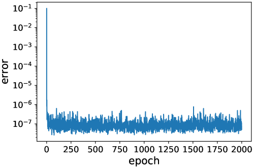
Fig. 1: Example 1: Training loss history.

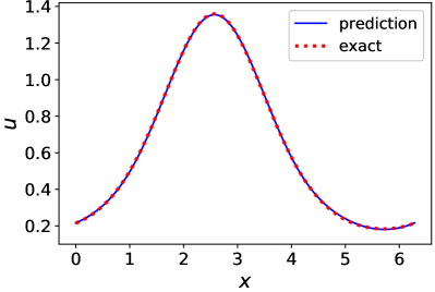
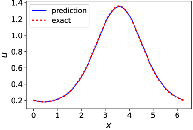
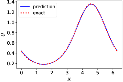
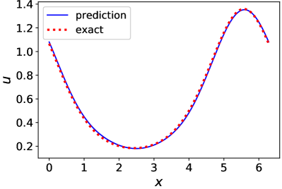
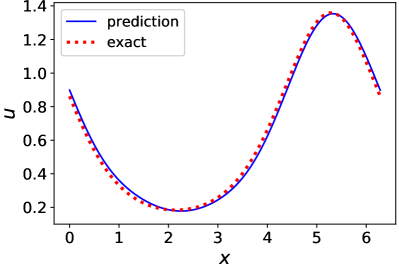
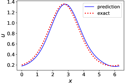
Fig. 2: Example 1: Comparison of the true solution and the learned model solution at different time. Top-left: $t=1$; top-right: $t=2$; middle-left: $t=3$; middle-right: $t=4$; bottom-left: $t=10$; bottom-right: $t=20$.

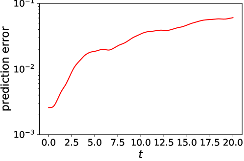
Fig. 3: Example 1: The evolution of the relative error in the prediction in $l^{2}$-norm.

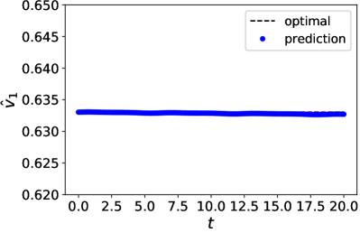
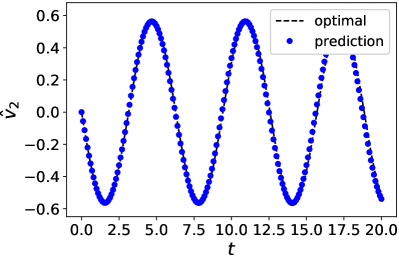
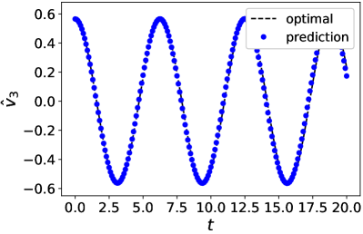
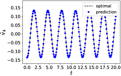
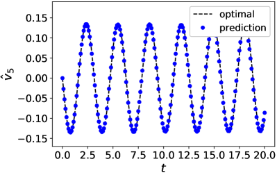
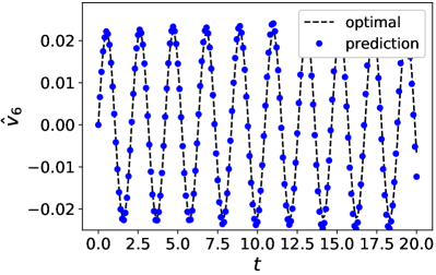
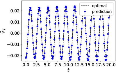
Fig. 4: Example 1: Evolution of the expansion coefficients for the learned model solution and the projection of the true solution.

5.2 Example 2: Diffusion Equation

We now consider the following diffusion equation with Dirichlet boundary condition:

$$\begin{cases}u_{t}=\sigma u_{xx},\quad(x,t)\in(0,\pi)\times\mathbb{R}^{+},\\ u(0,t)=u(\pi,t)=0,\quad t\in\mathbb{R}^{+}.\end{cases}$$ (33)

The finite dimensional approximation space is chosen as $\mathbb{V}_{n}={\rm span}\{\sin(jx),1\leq j\leq 5\}$, where $n=5$. (The symmetry of the problem allows this simplified choice to facilitate the computation and comparison.) The time lag $\Delta$ is taken as 0.1. The domain $D$ in the modal space is taken as $[-1,1]\times[-0.5,0.5]\times[-0.2,0.2]\times[-0.05,0.05]\times[-0.01,0.01]$, from which we sample $30,000$ training data. In this example, we employ a single-block ResNet method ($K=1$) containing 3 hidden layers of equal width of 30 neurons. The training of the network model is conducted for up to 500 epochs, where satisfactory convergence is established, as shown in Fig. 5. For validation and accuracy test, we conduct numerical predictions of the trained network model using initial condition

$$u_{0}(x)=\frac{x}{\pi}\left[5-\frac{4x}{\pi}-7\left(\frac{x}{\pi}\right)^{2}+6\left(\frac{x}{\pi}\right)^{3}\right],$$

for up to time $t=3$. Fig. 6 shows the solution predicted by the trained network model, along with the exact solution of the true equation (33). It can be seen that the predicted solution agrees well with the exact solution. The relative error in the numerical prediction is shown in Fig. 7, in term of $l^{2}$-norm. Finally, the evolution of the expansion coefficients is also shown given in Fig. 8. We observe that they agree well with the optimal coefficients obtained by projecting the exact solution onto the linear space $\mathbb{V}_{n}$.

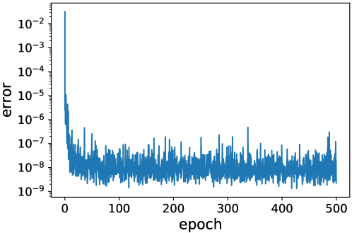
Fig. 5: Example 2: Training loss history.

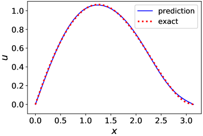
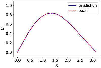
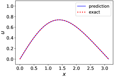
Fig. 6: Example 2: Comparison of the true solution and the learned model solution at different time. Top-left: $t=0$; top-right: $t=1$; bottom-left: $t=2$; bottom-right: $t=3$.

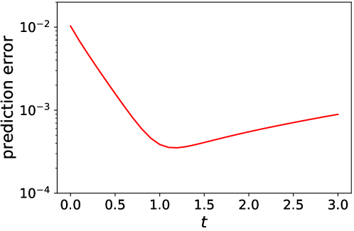
Fig. 7: Example 2: The evolution of the relative error in the prediction in $l^{2}$-norm.

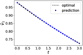
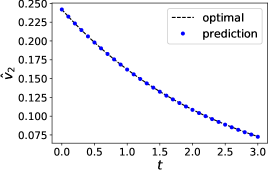
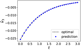
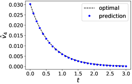
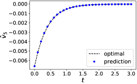
Fig. 8: Example 2: Evolution of the expansion coefficients for the learn model and the projection of the true solution.

We now consider the case of noisy data. All training data are then perturbed by a multiplicative factor $(1+\epsilon)$, where $\epsilon\sim[-\eta,\eta]$ follows uniform distribution. We consider two cases of $\eta=0.02$ and $\eta=0.05$, which respectively correspond to $\pm 2\%$ and $\pm 5\%$ relative noises in all data. In Fig. 9, the numerical solutions produced by the neural netwrok models are presented, after network training of $500$ epochs, along with the exact solution. We observe that the predictions of the network model are fairly robust against data noise. At higher level noises in data, the predictive results contain relatively larger numerical errors, as expected.

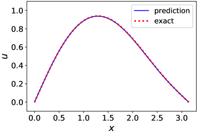
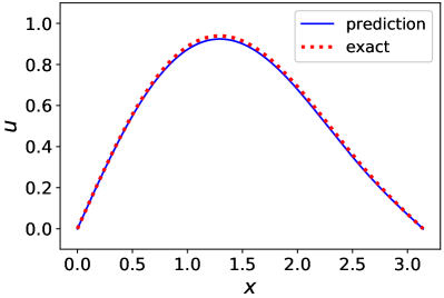
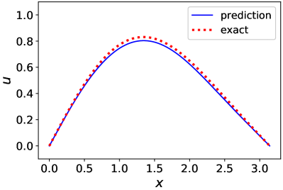
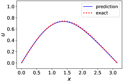
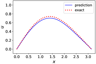
Fig. 9: Example 2: The solution at different time predicted by the neural network model trained with noisy data. Left: $2\%$ noise; right: $5\%$ noise. From top to bottom: solutions at $t=1$, $t=2$ and $t=3$, respectively.

5.3 Example 3: Viscous Burgers’ Equation

We now consider the viscous Burgers’ equation with Dirichlet boundary condition:

$$\begin{cases}u_{t}+\left(\frac{u^{2}}{2}\right)_{x}=\sigma u_{xx},\quad(x,t)\in(-\pi,\pi)\times\mathbb{R}^{+},\\ u(-\pi,t)=u(\pi,t)=0,\quad t\in\mathbb{R}^{+}.\end{cases}$$ (34)

We first consider a modestly large viscosity $\sigma=0.5$. The approximation space is chosen as $\mathbb{V}_{n}={\rm span}\{\sin(jx),1\leq j\leq 5\}$ with $n=5$. The time lag $\Delta$ is fixed at $\Delta=0.05$. The domain $D$ in the modal space is chosen as $[-1.5,1.5]\times[-0.2,0.2]\times[-0.05,0.05]\times[-0.01,0.01]\times[-0.002,0.002]$, from which $100,000$ training data are generated. The block ResNet method with two blocks ($K=2$) is used, where each block contains 3 hidden layers of equal width of 30 neurons. Upon training the network model satisfactorily (see Fig. 10 for the training loss history), we validate the trained model for the initial condition

$$u_{0}(x)=-\sin(x),$$

for time up to $t=2$. In Fig. 11, we compare the predicted solution against the exact solution at different time. The error of the prediction is computed and displayed in Fig. 12. We observe that the network model produces accurate prediction results. The learned expansion coefficients are shown in Fig. 13 and agree well with the optimal coefficients given by orthogonal projection of the exact solution.

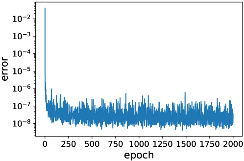
Fig. 10: Example 3: Training loss history.

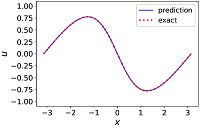
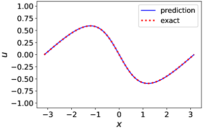
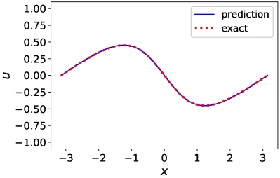
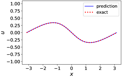
Fig. 11: Example 3: Comparison of the true solution, the learned model solution and the solution by Galerkin method at different time. Top-left: $t=0.5$; top-right: $t=1$; bottom-left: $t=1.5$; bottom-right: $t=2$.

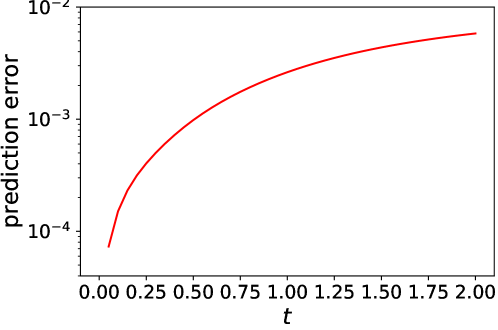
Fig. 12: Example 3: The evolution of the relative errors in the prediction in $l^{2}$-norm.

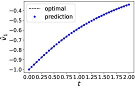
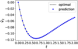
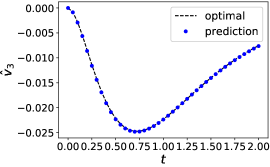
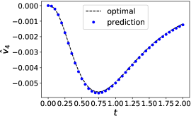
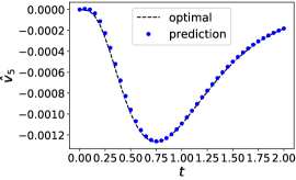
Fig. 13: Example 3: Evolution of the expansion coefficients for the learned model and the projection of the true solution.

We then consider a smaller viscosity $\sigma=0.1$. The approximation space is chosen to be relatively larger as $\mathbb{V}_{n}={\rm span}\{\sin(jx),1\leq j\leq 9\}$ with $n=9$. The time lag $\Delta$ is taken as 0.05. The domain $D$ in the modal space is taken as $[-1.5,1.5]\times[-0.5,0.5]\times[-0.2,0.2]^{2}\times[-0.1,0.1]^{2}\times[-0.05,0.05]^{2}\times[-0.02,0.02]$, from which we sample $500,000$ training data. In this example, we use the four-block ResNet method ($K=4$) with each block containing 3 hidden layers of equal width of 30 neurons. The network model is trained for up to 2,000 epochs, and training loss history is shown in Fig. 14. Then we validate the trained model for the initial condition

$$u_{0}(x)=-\sin(x).$$

In Fig. 15, we present the prediction results generated by the trained network, for time up to $t=2$. One can see that the predicted solutions are very close to the exact ones, This can also be seen in the relative error of the prediction from Fig. 16. We note that at time $t=2$ the exact solution develops a relatively sharp (albeit still smooth) transition layer at this relatively low visocity. The numerical solution starts to exhibit Gibbs’ type small oscillations. This is a rather common feature for global type approximation and is not unexpected. Comparison between the learned and optimal expansion coefficients is also shown in Fig. 17.

Fig. 14: Example 3: Training loss history.

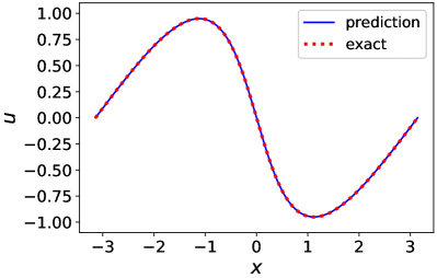
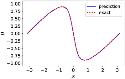
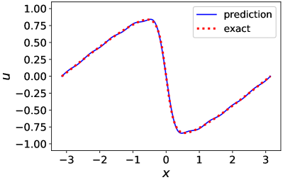
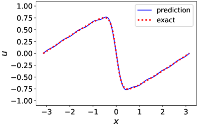
Fig. 15: Example 3: Comparison of the true solution, the learned model solution and the solution by Galerkin method at different time. Top-left: $t=0.5$; top-right: $t=1$; bottom-left: $t=1.5$; bottom-right: $t=2$.

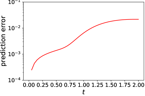
Fig. 16: Example 3: The evolution of the relative error in prediction in $l^{2}$-norm.

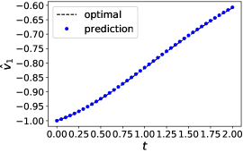
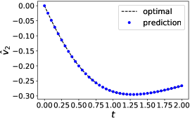
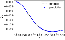
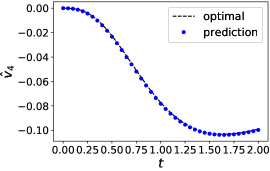
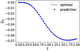
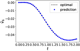
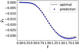
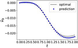
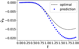
Fig. 17: Example 3: Evolution of the expansion coefficients for the learned model solution and the projection of the true solution.

5.4 Example 4: Inviscid Burgers’ Equation

We now consider the inviscid Burgers’ equation with Dirichlet boundary condition:

$$\begin{cases}u_{t}+\left(\frac{u^{2}}{2}\right)_{x}=0,\quad(x,t)\in(-\pi,\pi)\times\mathbb{R}^{+},\\ u(-\pi,t)=u(\pi,t)=0,\quad t\in\mathbb{R}^{+}.\end{cases}$$ (35)

This represents a challenging problem, as the nonlinear hyperbolic nature of this equation can produce shocks over time even if the initial solution is smooth.

The approximation space is chosen as $\mathbb{V}_{n}={\rm span}\{\sin(jx),1\leq j\leq 9\}$ with $n=9$. The time lag $\Delta$ is taken as $0.05$. The domain $D$ in the modal space is taken as $[-1.1,1.1]\times[-0.5,0.5]\times[-0.3\times 0.3]^{7}$, from which we sample $1,000,000$ training data. We remark that by sampling in this manner, all of our training data are smooth. In this example, we use the block ResNet method with $K=4$ blocks, each of which contains 3 hidden layers of equal width of 30. The network training is conducted for up to $2,000$ epochs, when it was deemed satisfactory, as shown in the loss history in Fig. 18. For validation, we conduct system prediction using initial condition

$$u_{0}(x)=-\sin(x),$$

for time up to $t=2$. Although the initial condition is smooth, the exact solution will start to develop shock at $t=1$.

The prediction results generated by our network model are shown in Fig. 19, along with the exact solution, and the Galerkin solution of the Burgers’ equation using the same linear space $\mathbb{V}_{n}$. Due to the discontinuity in the solution, Gibbs type oscillations appear in the predicted solutions. This is not unexpected, as the best representation of a discontinuous function using the linear subspace $\mathbb{V}_{n}$ will naturally produce oscillations, unless special treatment such as filtering is utilized (which is not pursued in this work). The Galerkin solution of the equation (35) exhibits the similar Gibbs’ oscillations for precisely the same reason. We remark that it can be seen that our neural network prediction is visibly better than the Galerkin solution. While the network prediction is entirely data driven and does not require knowledge of the equation, the Galerkin solution is attainable only after knowing the precise form of the governing equation. In Fig. 21, we plot the evolution of the expansion coefficients in the modal space obtained by the neural network model prediction, Galerkin solution of the Burgers’ equation, and orthogonal projection of the exact solution (denoted as “optimal”), the last of which serves as the reference solution. It is clearly seen that the neural network model produces more accurate results than the Galerkin solver. The accuracy improvement is especially visible at higher modes such as $\hat{v}_{7}$, $\hat{v}_{8}$, and $\hat{v}_{9}$. The cause of the accuracy improvement over Galerkin method will be pursued in a separate work.

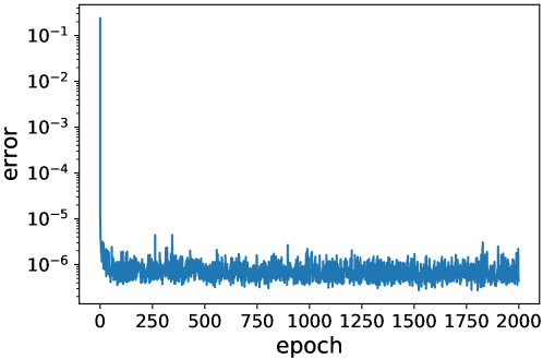
Fig. 18: Example 4: Training loss history.

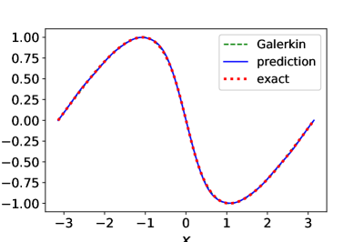
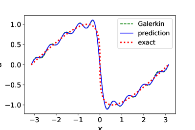
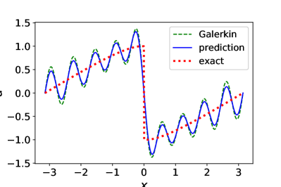
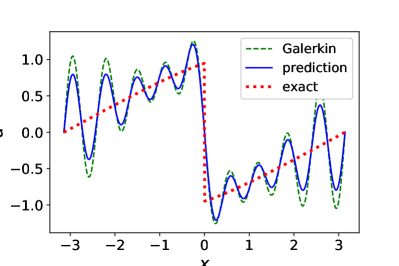
Fig. 19: Example 4: Comparison of the true solution, the learned model solution and the solution by Galerkin method at different time. Top-left: $t=0.5$; top-right: $t=1$; bottom-left: $t=1.5$; bottom-right: $t=2$.

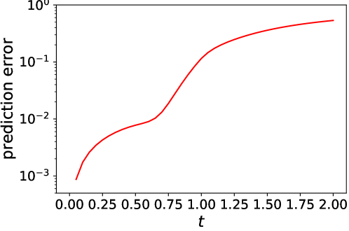
Fig. 20: Example 4: The evolution of the relative error in the prediction in $l^{2}$-norm.

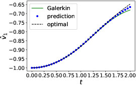
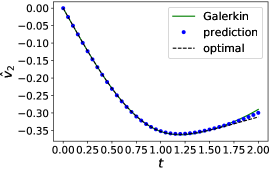
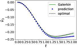
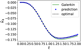
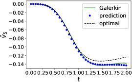
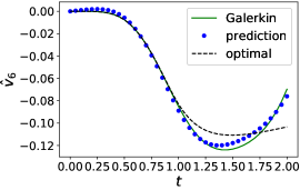
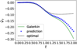
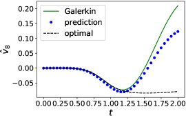
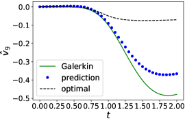
Fig. 21: Example 4: Evolution of the expansion coefficients for the learned model solution and the projection of the true solution.

5.5 Example 5: Two-Dimensional Convection-Diffusion Equation

In our last example, we consider a two-dimensional convection-diffusion equation to demonstrate the applicability of the proposed algorithm for multiple dimensions. The equation set up is as follows.

$$\begin{cases}u_{t}+\alpha_{1}u_{x}+\alpha_{2}u_{y}=\sigma_{1}u_{xx}+\sigma_{2}u_{yy},\quad(x,y,t)\in(-\pi,\pi)^{2}\in\mathbb{R}^{+}\\ u(-\pi,y,t)=u(\pi,y,t),~{}u_{x}(-\pi,y,t)=u_{x}(\pi,y,t),~{}~{}(y,t)\in(-\pi,\pi)\times\mathbb{R}^{+},\\ u(x,-\pi,t)=u(x,\pi,t),~{}u_{y}(x,-\pi,t)=u_{y}(x,\pi,t),~{}~{}(x,t)\in(-\pi,\pi)\times\mathbb{R}^{+},\end{cases}$$ (36)

where the parameters are set as $\alpha_{1}=1$, $\alpha_{2}=0.7$, $\sigma_{1}=0.1$, and $\sigma_{2}=0.16$ in the test.

We chose the finite dimensional approximation space $\mathbb{V}_{n}$ as a span by $n=25$ basis functions:

$$\phi_{1}(x,y)=1,\quad\phi_{2}(x,y)=\cos(x),\quad\phi_{3}(x,y)=\sin(x),$$

$$\phi_{4}(x,y)=\cos(2x),\quad\phi_{5}(x,y)=\sin(2x),\quad\phi_{6}(x,y)=\cos(3x),\quad\phi_{7}(x,y)=\sin(3x),$$

$$\phi_{8}(x,y)=\cos(y),\quad\phi_{9}(x,y)=\sin(y),\quad\phi_{10}(x,y)=\cos(2y),\quad\phi_{11}(x,y)=\sin(2y),$$

$$\phi_{12}(x,y)=\cos(3y),\quad\phi_{13}(x,y)=\sin(3y),\quad\phi_{14}(x,y)=\cos(x)\cos(y),$$

$$\phi_{15}(x,y)=\cos(x)\sin(y),\quad\phi_{16}(x,y)=\sin(x)\cos(y),\quad\phi_{17}(x,y)=\sin(x)\sin(y),$$

$$\phi_{18}(x,y)=\cos(x)\cos(2y),\quad\phi_{19}(x,y)=\cos(x)\sin(2y),\quad\phi_{20}(x,y)=\sin(x)\cos(2y),$$

$$\phi_{21}(x,y)=\sin(x)\sin(2y),\quad\phi_{22}(x,y)=\cos(2x)\cos(y),\quad\phi_{23}(x,y)=\cos(2x)\sin(y),$$

$$\phi_{24}(x,y)=\sin(2x)\cos(y),\quad\phi_{25}(x,y)=\sin(2x)\sin(y).$$

The time lag $\Delta$ is taken as 0.1 and $1,000,000$ training data are generated. The neural network model is a five-block ResNet method ($K=5$) with each block containing 3 hidden layers of equal width of 40 neurons. Upon training the network model satisfactorily for 400 epochs (see Fig. 22 for the training loss history), we validate the trained models by using the initial condition

$$u_{0}(x)=\frac{2}{5}\exp\left(\frac{\sin(x)-\cos(y)}{2}\right),$$

for time up to $t=3$.

The comparison between the network model prediction and the exact solution is shown in Figs. 23 as solution contours, and in Fig. 24 as solution slice profiles at certain locations. The relative error in the network prediction is shown in Fig. 25. The time evolution of the modal expansion coefficients is shown in Fig. 26, along with the evolution of the orthogonal projection coefficients of the exact solution. Again, we observe good accuracy in the network prediction.

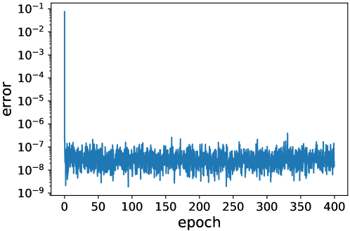
Fig. 22: Example 5: Training loss history.

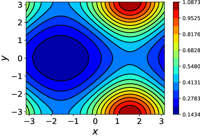
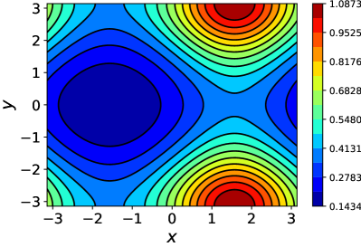
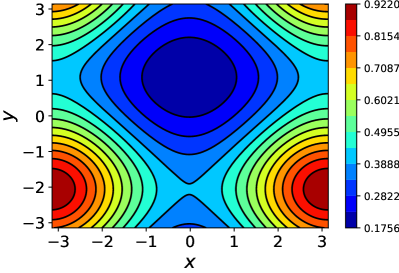
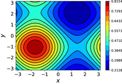
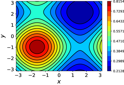
Fig. 23: Example 5: Contour plots of the solutions at different time. From top to bottom $t=0,$ $t=1.5$ and $t=3$. Left: learned model solution; right: true solution. 15 equally spaced contour lines are shown at the same levels for the learned model solution and true solution.

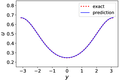
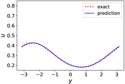
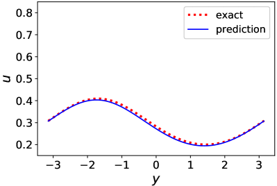
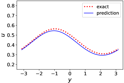
Fig. 24: Example 5: Comparison of the true solution and the learned model solution at different time along the line $x=0$. Top-left: $t=0$; top-right: $t=1$; bottom-left: $t=2$; bottom-right: $t=3$.

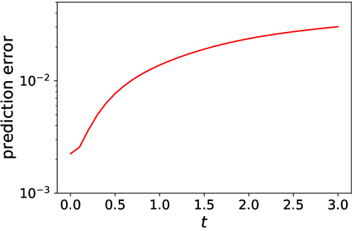
Fig. 25: Example 5: The evolution of the relative error in the prediction in $l^{2}$-norm.

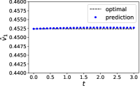
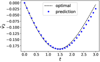
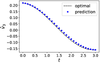
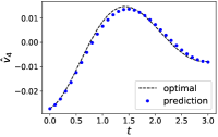
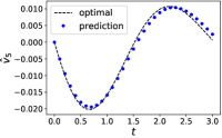
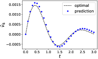
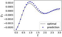
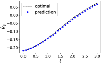
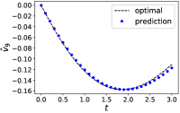
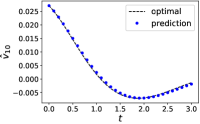
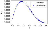
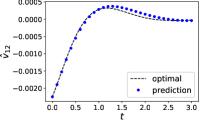
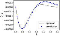
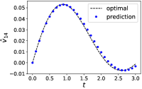
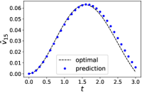
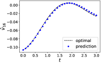
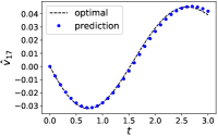
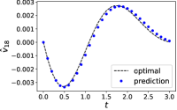
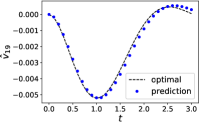
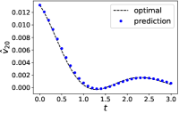
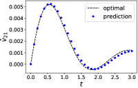
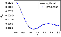
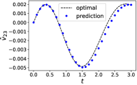
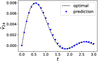
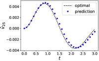
Fig. 26: Example 5: Evolution of the expansion coefficients for the learned model solution and the projection of the true solution.

6 Conclusion

In this paper, we presented a data-driven framework for learning unknown time-dependent autonomous PDEs, based on training of deep neural networks, particularly, those based on residual networks. Instead of identifying the exact terms in the underlying PDEs forms of the unknown PDEs, we proposed to approximately recover the evolution operator of the underlying PDEs. Since the evolution operator completely characterizes the solution evolution, its recovery allows us to conduct accurate system prediction by recursive use of the operator. The key to the successful learning of the operator is to reduce the problem into finite dimension. To this end, we proposed an approach in modal space, i.e., generalized Fourier space. Error analysis was conducted to quantify the prediction accuracy of the proposed data-driven approach. We presented a variety of test problems to demonstrate the applicability and potential of the method. More detailed study of its properties, as well as its applications to more complex problems, will be pursued in future study.

References

- [1] M. Abadi, A. Agarwal, P. Barham, E. Brevdo, Z. Chen, C. Citro, G. S. Corrado, A. Davis, J. Dean, M. Devin, S. Ghemawat, I. Goodfellow, A. Harp, G. Irving, M. Isard, Y. Jia, R. Jozefowicz, L. Kaiser, M. Kudlur, J. Levenberg, D. Mané, R. Monga, S. Moore, D. Murray, C. Olah, M. Schuster, J. Shlens, B. Steiner, I. Sutskever, K. Talwar, P. Tucker, V. Vanhoucke, V. Vasudevan, F. Viégas, O. Vinyals, P. Warden, M. Wattenberg, M. Wicke, Y. Yu, and X. Zheng, TensorFlow: Large-scale machine learning on heterogeneous systems, 2015, https://www.tensorflow.org/. Software available from tensorflow.org.
- [2] J. Bongard and H. Lipson, Automated reverse engineering of nonlinear dynamical systems, Proc. Natl. Acad. Sci. U.S.A., 104 (2007), pp. 9943–9948.
- [3] S. L. Brunton, B. W. Brunton, J. L. Proctor, E. Kaiser, and J. N. Kutz, Chaos as an intermittently forced linear system, Nature Communications, 8 (2017).
- [4] S. L. Brunton, J. L. Proctor, and J. N. Kutz, Discovering governing equations from data by sparse identification of nonlinear dynamical systems, Proc. Natl. Acad. Sci. U.S.A., 113 (2016), pp. 3932–3937.
- [5] S. Chan and A. Elsheikh, A machine learning approach for efficient uncertainty quantification using multiscale methods, J. Comput. Phys., 354 (2018), pp. 494–511.
- [6] J. Han, A. Jentzen, and W. E, Solving high-dimensional partial differential equations using deep learning, Proceedings of the National Academy of Sciences, 115 (2018), pp. 8505–8510.
- [7] K. He, X. Zhang, S. Ren, and J. Sun, Deep residual learning for image recognition, in Proceedings of the IEEE conference on computer vision and pattern recognition, 2016, pp. 770–778.
- [8] J. Hesthaven and S. Ubbiali, Non-intrusive reduced order modeling of nonlinear problems using neural networks, J. Comput. Phys., 363 (2018), pp. 55–78.
- [9] S. H. Kang, W. Liao, and Y. Liu, IDENT: Identifying differential equations with numerical time evolution, arXiv preprint arXiv:1904.03538, (2019).
- [10] S. Karumuri, R. Tripathy, I. Bilionis, and J. Panchal, Simulator-free solution of high-dimensional stochastic elliptic partial differential equations using deep neural networks, arXiv preprint arXiv:1902.05200, (2019).
- [11] Y. Khoo, J. Lu, and L. Ying, Solving parametric PDE problems with artificial neural networks, arXiv preprint arXiv:1707.03351, (2018).
- [12] Z. Long, Y. Lu, and B. Dong, PDE-Net 2.0: Learning PDEs from data with a numeric-symbolic hybrid deep network, arXiv preprint arXiv:1812.04426, (2018).
- [13] Z. Long, Y. Lu, X. Ma, and B. Dong, PDE-net: Learning PDEs from data, in Proceedings of the 35th International Conference on Machine Learning, J. Dy and A. Krause, eds., vol. 80 of Proceedings of Machine Learning Research, Stockholmsmässan, Stockholm Sweden, 10–15 Jul 2018, PMLR, pp. 3208–3216.
- [14] N. M. Mangan, J. N. Kutz, S. L. Brunton, and J. L. Proctor, Model selection for dynamical systems via sparse regression and information criteria, Proceedings of the Royal Society of London A: Mathematical, Physical and Engineering Sciences, 473 (2017).
- [15] D. Nguyen, S. Ouala, L. Drumetz, and R. Fablet, EM-like learning chaotic dynamics from noisy and partial observations, arXiv preprint arXiv:1903.10335, (2019).
- [16] S. Pawar, S. M. Rahman, H. Vaddireddy, O. San, A. Rasheed, and P. Vedula, A deep learning enabler for nonintrusive reduced order modeling of fluid flows, Physics of Fluids, 31 (2019), p. 085101.
- [17] T. Qin, K. Wu, and D. Xiu, Data driven governing equations approximation using deep neural networks, J. Comput. Phys., 395 (2019), pp. 620 – 635.
- [18] M. Raissi, Deep hidden physics models: Deep learning of nonlinear partial differential equations, Journal of Machine Learning Research, 19 (2018), pp. 1–24.
- [19] M. Raissi and G. E. Karniadakis, Hidden physics models: Machine learning of nonlinear partial differential equations, Journal of Computational Physics, 357 (2018), pp. 125 – 141.
- [20] M. Raissi, P. Perdikaris, and G. E. Karniadakis, Machine learning of linear differential equations using gaussian processes, J. Comput. Phys., 348 (2017), pp. 683–693.
- [21] M. Raissi, P. Perdikaris, and G. E. Karniadakis, Physics informed deep learning (part i): Data-driven solutions of nonlinear partial differential equations, arXiv preprint arXiv:1711.10561, (2017).
- [22] M. Raissi, P. Perdikaris, and G. E. Karniadakis, Physics informed deep learning (part ii): Data-driven discovery of nonlinear partial differential equations, arXiv preprint arXiv:1711.10566, (2017).
- [23] M. Raissi, P. Perdikaris, and G. E. Karniadakis, Multistep neural networks for data-driven discovery of nonlinear dynamical systems, arXiv preprint arXiv:1801.01236, (2018).
- [24] D. Ray and J. Hesthaven, An artificial neural network as a troubled-cell indicator, J. Comput. Phys., 367 (2018), pp. 166–191.
- [25] S. H. Rudy, S. L. Brunton, J. L. Proctor, and J. N. Kutz, Data-driven discovery of partial differential equations, Science Advances, 3 (2017), p. e1602614.
- [26] S. H. Rudy, J. N. Kutz, and S. L. Brunton, Deep learning of dynamics and signal-noise decomposition with time-stepping constraints, J. Comput. Phys., 396 (2019), pp. 483–506.
- [27] H. Schaeffer, Learning partial differential equations via data discovery and sparse optimization, Proceedings of the Royal Society of London A: Mathematical, Physical and Engineering Sciences, 473 (2017).
- [28] H. Schaeffer and S. G. McCalla, Sparse model selection via integral terms, Phys. Rev. E, 96 (2017), p. 023302.
- [29] H. Schaeffer, G. Tran, and R. Ward, Extracting sparse high-dimensional dynamics from limited data, SIAM Journal on Applied Mathematics, 78 (2018), pp. 3279–3295.
- [30] M. Schmidt and H. Lipson, Distilling free-form natural laws from experimental data, Science, 324 (2009), pp. 81–85.
- [31] Y. Sun, L. Zhang, and H. Schaeffer, NeuPDE: Neural network based ordinary and partial differential equations for modeling time-dependent data, arXiv preprint arXiv:1908.03190, (2019).
- [32] R. Tibshirani, Regression shrinkage and selection via the lasso, Journal of the Royal Statistical Society. Series B (Methodological), (1996), pp. 267–288.
- [33] G. Tran and R. Ward, Exact recovery of chaotic systems from highly corrupted data, Multiscale Model. Simul., 15 (2017), pp. 1108–1129.
- [34] R. Tripathy and I. Bilionis, Deep UQ: learning deep neural network surrogate model for high dimensional uncertainty quantification, J. Comput. Phys., 375 (2018), pp. 565–588.
- [35] Y. Wang and G. Lin, Efficient deep learning techniques for multiphase flow simulation in heterogeneous porous media, arXiv preprint arXiv:1907.09571, (2019).
- [36] Y. Wang, Z. Shen, Z. Long, and B. Dong, Learning to discretize: Solving 1D scalar conservation laws via deep reinforcement learning, arXiv preprint arXiv:1905.11079, (2019).
- [37] K. Wu, T. Qin, and D. Xiu, Structure-preserving method for reconstructing unknown hamiltonian systems from trajectory data, arXiv preprint arXiv:1905.10396, (2019).
- [38] K. Wu and D. Xiu, Numerical aspects for approximating governing equations using data, J. Comput. Phys., 384 (2019), pp. 200–221.
- [39] Y. Zhu and N. Zabaras, Bayesian deep convolutional encoder-decoder networks for surrogate modeling and uncertainty quantification, J. Comput. Phys., 366 (2018), pp. 415–447.