Near wall patch representation of wall bounded turbulence

Abstract

Recent experimental and computational studies indicate that near wall turbulent flows can be characterized by universal small scale autonomous dynamics that are modulated by large scale structures. We formulate numerical simulations of near wall turbulence in a small domain localized to the boundary, whose size scales in viscous units. To mimic the environment in which the near wall turbulence evolves, the formulation accounts for the flux of mean momentum through the upper boundary of the domain. Comparisons of the model’s two dimensional energy spectra and low order single-point statistics with the corresponding quantities computed from direct numerical simulations indicate that it successfully captures the dynamics of the small scale near wall turbulence.

1 Introduction

High Reynolds number wall bounded turbulent shear flows are characterized by a separation of scales between the flow in the near-wall region, in which mean viscous stresses play an important role, and the flow farther away from the wall, where mean viscous effects are largely negligible. This separation of scales is quantified by the friction Reynolds number $Re_{\tau}=\delta/\delta_{\nu}$, where $\delta$ is the characteristic length scale of the shear layer, such as a channel half-width, a pipe radius, or a boundary layer thickness, and $\delta_{\nu}=\nu/u_{\tau}$ is the viscous length scale, where $\nu$ is the kinematic viscosity of the fluid, $u_{\tau}=\sqrt{\tau_{w}/\rho}$, $\tau_{w}$ is the mean wall shear stress, and $\rho$ is the fluid density. Both the direct numerical simulation (DNS) and large eddy simulation (LES) of such wall bounded turbulent flows are expensive, as the spatial degrees of freedom required to resolve the near-wall layer scale as $\mathcal{O}(Re_{\tau}^{2.5})$ and $\mathcal{O}(Re_{\tau}^{2})$ for DNS and LES, respectively (Mizuno & Jiménez, 2013). For a large class of flows of technological importance, this cost is prohibitive, even on modern high-performance computing systems.

Thanks to advances in experimental techniques and computational power, the understanding of the physics of wall bounded flows has increased greatly since the earliest investigations by Hagen (1839), Darcy (1854), and Reynolds (1895), and the later work by Millikan (1938). It is well known that there is an autonomous near-wall cycle of self sustaining mechanisms (Jiménez & Moin, 1991; Hamilton et al., 1995; Jeong et al., 1997), involving low and high speed streamwise velocity streaks and coherent structures of quasi-streamwise vorticity. Jiménez & Pinelli (1999) showed that this cycle of near-wall dynamics persists without any input from the turbulence farther away from the wall. Moreover, if any element of the cycle is suppressed, the near-wall turbulent kinetic energy (TKE) decays, and the flow becomes laminar. However, the large-scale structures (superstructures) in the outer layer do modulate the turbulent fluctuations in the near-wall region (Hutchins & Marusic, 2007; Marusic et al., 2010a; Ganapathisubramani et al., 2012), leaving their “footprint” on the autonomous cycle. Mathis et al. (2011) (see also references therein) modulated a “universal signal” identified in experimental data as the contribution of the small-scale near-wall turbulence, to formulate a predictive statistical model. The large-scale modulation results, for instance, in an $Re_{\tau}$-dependent peak of the turbulent kinetic energy in the near-wall region (see figure 1) because its influence increases with increasing $Re_{\tau}$ (DeGraaff & Eaton, 2000).

Recently, Lee & Moser (2019) performed spectral analysis of channel flow DNS data for several different $Re_{\tau}$ (ranging from approximately $550$ to $5200$) to investigate the relative importance of different length scales to the production, transport, and dissipation of TKE. Their results suggest that the small scales in the near-wall region behave universally. Indeed, when the energy spectrum is high-pass filtered to only include contributions from wavenumbers with magnitude larger than some $k_{\rm cut}\delta_{\nu}=0.00628$ (corresponding to a wavelength $\lambda_{\rm cut}/\delta_{\nu}=1000$), the resulting energy is found to be independent of $Re_{\tau}$, as shown in figure 1. Similar results were also obtained in Samie et al. (2018) for experimental data ranging from $Re_{\tau}\approx 6000-20000$.

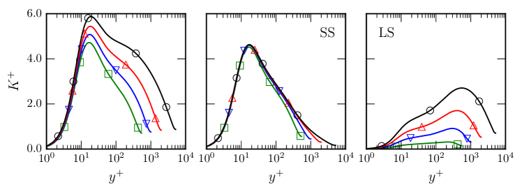
Figure 1: Unfiltered, high-pass (SS), and low pass (LS) portion of the turbulent kinetic energy scaled in viscous units with $k_{\text{cut}}\delta_{\nu}=0.00628$ ($\lambda_{\text{cut}}/\delta_{\nu}=1000$) for a channel flow at various $Re_{\tau}$ (green: $Re_{\tau}=550$, blue: $Re_{\tau}=1000$, red: $Re_{\tau}=2000$, black: $Re_{\tau}=5200$). The contributions from the large scales increases with $Re_{\tau}$, but the contribution from the small scales is largely independent of $Re_{\tau}$. Figure reproduced from Lee & Moser (2019) with permission.

These works, along with those mentioned above, indicate that the near-wall region has universal small scales, independent of $Re_{\tau}$. The large scale portion of the near-wall turbulence, however, is the result of eddies whose size and influence on the turbulent statistics depend on $Re_{\tau}$. These observations suggest that an appropriately formulated numerical simulation of only the small-scale near-wall dynamics should be able to reproduce the near-wall small-scale statistics (e.g. SS in figure 1). One objective of the work reported here is to test this hypothesis.

With this in mind, we endeavor to design a computational model of the universal near-wall small scales of turbulent, wall bounded shear flows. The primary modeling goal is to accurately represent the contribution of the small scales to the near-wall turbulent statistics without simulating the entire wall-bounded turbulent shear flow. The model is formulated to simulate wall bounded turbulence only in a near-wall, rectangular domain $\Omega$ localized to the boundary. The size of the domain scales in viscous units, so that as $Re_{\tau}$ increases, the domain shrinks in size relative to the size of the overall flow whose near-wall turbulence is being modeled.

The model is formulated to mimic the mean flux of momentum from the outer layer, but it otherwise “isolates”, or decouples, the near wall-wall dynamics from large-scale outer-layer influences, such as the modulations by superstructures. In this way it is similar to the numerical experiments described in Jiménez & Pinelli (1999) in which the equations of motion are filtered to suppress the dynamics above some fixed wall-normal height. It is fundamentally different from a low Reynolds number channel flow, for example, whose dynamics are influenced by the presence of the opposite wall. If such a configuration can accurately model the dynamics of the near-wall, small scale features of the flow, it could be used to study the response of near-wall turbulence to changes in the momentum environment, including the effects of pressure gradients. Further, assuming a separation of scales between the small-scale autonomous near-wall dynamics and the large-scale outer turbulence that modulates it, the model flow could be used to inform a representation of wall turbulence in a wall-modeled large eddy simulation.

This paper reports on the development and evaluation of just such a computational model of the near-wall layer in turbulent shear flows. It originated as a design for the high-fidelity, “microscale” component of a multiscale computational approach for simulating wall bounded turbulence in the style of the heterogeneous multiscale method (Abdulle et al., 2012), as pursued by Sandham et al. (2017), who coupled their microscale model to a large eddy simulation (LES) in a full channel. Previous multiscale approaches of this type include Pascarelli et al. (2000) and Tang & Akhavan (2016), in which large eddy simulations are coupled to minimal flow unit simulations. One application of the model will be to generate data to inform a pressure-gradient-dependent wall model for an LES (Piomelli & Balaras, 2002; Bose & Park, 2018), as suggested by Coleman et al. (2015). In this case, the model plays the role of the universal signal in Mathis et al. (2011). Additionally, the current model approach could be used to study the interaction between the small, near-wall turbulent dynamics and more complicated physical processes, such as heat transfer, chemical reactions, turbophoresis, or surface roughness.

The rest of the manuscript is organized as follows: section 2 contains a description of the computational model and the numerical method used to integrate the equations of motion. Section 3 provides a comparison between the statistics generated by the model and the corresponding quantities from DNS for the cases of both zero and mild favorable pressure gradients. In section 4 the results are summarized, and possible applications and extensions of the model are discussed.

2 Formulation

2.1 Notation

In the following discussion, the velocity components in the streamwise (x), wall-normal (y) and spanwise (z) directions are denoted as $u$, $v$, and $w$, respectively, and when using index notation, these directions are labeled 1, 2, and 3, respectively. The expected value is denoted with angle brackets (as in $\langle\cdot\rangle$), and upper case $U$ and $P$ indicate the mean velocity and pressure, so that $\langle u_{i}\rangle=U_{i}$. The velocity and pressure fluctuations are indicated with primes, e.g. $u_{i}=U_{i}+u_{i}^{\prime}$. Partial derivatives shortened to $\partial_{i}$ signify $\partial/\partial x_{i}$, differentiation in the direction $x_{i}$. The mean advective derivative is $D(\cdot)/Dt=\partial_{t}(\cdot)+U_{j}\partial_{j}(\cdot)$, where Einstein summation notation is implied. In general, repeated indices imply summation, with the exception of repeated Greek indices. Lastly, the superscript ‘$+$’ denotes non-dimensionalisation with the kinematic viscosity $\nu$ and the friction velocity $u_{\tau}$.

2.2 Motivation

Figure 2: The fluid is subject to periodic boundary conditions at the (dash-dotted) side walls, constant Dirichlet/Neumann conditions at the upper boundary $y=2H$, and the no-slip condition at the wall $y=0$, as described in (1). In addition to the constant pressure gradient assumed to be present in the near wall layer, the model includes an auxiliary pressure gradient in a “fringe region” to account for momentum transport at the computational boundary $y=2H$.

Intrinsic to the computational model is the assumption of a separation of temporal and spatial scales between the small-scale turbulence arising from the autonomous near-wall dynamics and the large-scale outer-layer turbulence. The near-wall dynamics can therefore be considered to be in local equilibrium with the pressure gradient and momentum flux environment in which they are evolving. Furthermore, under this scale-separation assumption, both the local pressure gradient and the turbulent momentum flux from the outer layer toward the wall can be considered constants on the scale of the near-wall dynamics being simulated. Note that despite this assumption, the near-wall model will be representative of the wall layer in wall bounded flows that are not in equilibrium overall, or those with non-constant pressure gradients. The assumptions break down, for example, for a boundary layer near separation.

The goal of the computational model is to simulate the turbulent small scales in the near wall region as a function of an imposed pressure gradient only in a small, rectangular domain localized to the boundary. This necessarily means placing nonphysical computational boundaries in a region of chaotic, highly nonlinear dynamics. In addition to the standard no-slip condition at the lower boundary $y=0$, the use of periodic boundary conditions at the side-walls is well established, assuming the flow is statistically homogeneous in these directions. The problem of prescribing appropriate boundary conditions at the upper computational boundary, however, is nontrivial (Berselli et al., 2006; Sagaut et al., 2006). Once a mathematically well posed condition is prescribed, care must be taken to prevent the approximation inherent in the boundary condition from polluting the turbulent dynamics in the domain’s interior. To address this issue, the model augments the near wall computational domain with a “fringe region.” In this fringe region, the flow is externally forced to account for the mean flux of momentum through the upper computational boundary that is precluded by the boundary conditions imposed there. The inclusion of such a region increases the computational cost of the model, but it provides the momentum transport needed to create the “correct environment” for the evolution of turbulence in the near wall region. In this way, the fringe region mollifies the effect of the nonphysical computational boundary. Similar techniques are used for designing inflow/outflow conditions in the DNS of turbulent boundary layers (Khujadze & Oberlack, 2004; Colonius, 2004; Wu & Moin, 2009; Sillero et al., 2013), for example, as well as in molecular dynamics simulations, often referred to as a “heat-bath” or “thermostat” (Berendsen et al., 1984; Yong & Zhang, 2013).

If one is interested in the turbulent statistics resulting from a constant pressure gradient near wall region out to a wall-normal height of $y\approx H$, the fringe region consists of a layer from $H\leq y\leq 2H$ in which a horizontally uniform streamwise forcing is applied, as illustrated in figure 2.

2.3 Mathematical formulation

The near wall patch (NWP) model is defined by the equations of motion and boundary conditions in the rectangular domain $\Omega=[0,L_{x}]\times[0,L_{y}]\times[0,L_{z}]$:

$$\begin{cases}\begin{array}[]{rr}\partial_{t}u_{i}+u_{j}\partial_{j}u_{i}+\partial_{i}p-\nu\partial_{j}\partial_{j}u_{i}=f_{i}-\partial_{i}P&\text{in }\Omega\\ \partial_{i}u_{i}=0&\text{in }\Omega\\ \partial_{i}P=dP/dx\,\,\delta_{i1}\text{ is constant}&\text{in }\Omega\\ u_{i}\text{ periodic in }x\text{ and }z\text{ directions}&\text{in }\Omega\\ u_{i}=0&y=0\\ v=\partial_{y}w=0&y=L_{y}\\ \partial_{y}u=\psi\in\mathbb{R}&y=L_{y}\\ f_{i}(x,y,z,t)=f(y)\,\delta_{i1}&\text{in }\Omega.\end{array}\end{cases}$$ (1)

These are simply the forced incompressible Navier Stokes equations on a periodic domain in the wall-parallel directions, with the no-slip boundary condition at $y=0$ (the wall), and no-flow through and constant viscous tangential traction $\nu\,\psi$ in the streamwise direction ($x$) specified at the top $y=L_{y}$. The term $dP/dx$ models the externally imposed streamwise pressure gradient in the real turbulent flow being modeled, which is constant on the scale of the NWP. The pressure $p$ is the NWP model’s pressure field, which is determined from the incompressibility constraint, in the usual way. It only remains to specify $\psi$ and the forcing function $f(y)$. The former represents the viscous flux of momentum through the top, and the latter is a source of streamwise momentum that makes up for the missing turbulent flux of streamwise momentum through the upper computational boundary, owing to the boundary conditions that imply that the Reynolds stress vanishes there.

The forcing function $f(y)$ is non-zero only in the fringe region $y>L_{y}/2$, and is constructed such that

$$\int_{0}^{L_{y}}f(y)\,dy=-\tau_{\rm turb},$$ (2)

where $\tau_{\rm turb}$ is the turbulent flux of mean momentum through $y=L_{y}$ in the turbulent flow being modeled.

In the real turbulent flow with a (locally) constant mean pressure gradient, the mean streamwise momentum equation integrated over $[0,L_{y}]$ yields:

$$-\frac{dP}{dx}L_{y}+\left(\left.\nu\frac{\partial U}{\partial y}\right|_{y=L_{y}}-\tau_{\rm turb}\right)-\tau_{w}=0$$ (3)

$$\implies\tau_{w}=-\frac{dP}{dx}L_{y}+\tau_{\rm top}$$ , (4)

The term in parentheses, $\tau_{\rm top}$, is the total momentum flux (viscous plus turbulent) through $y=L_{y}$, and it, along with $dP/dx$, determines the mean wall shear stress $\tau_{w}$.

The mean streamwise stress balance for the NWP model system (1) is

$$\nu\frac{\partial U}{\partial y}-\left\langle u^{\prime}v^{\prime}\right\rangle+\int_{0}^{y}f(s)ds=y\frac{dP}{dx}+\tau_{w}.$$ (5)

The boundary conditions in (1) and the constraint (2) imply that at $y=L_{y}$, (5) becomes

$$\nu\psi+\int_{0}^{L_{y}}f(s)ds=L_{y}\frac{dP}{dx}+\tau_{w}$$ (6)

$$\implies\tau_{w}=-\frac{dP}{dx}L_{y}+\nu\psi-\tau_{\rm turb}$$ , (7)

so that for fixed $L_{y}$, the parameters $\nu$, $\tau_{\rm turb}$, $\psi$, and $dP/dx$ determine $\tau_{w}$. Dimensional analysis therefore implies that there is a two-parameter family of possible turbulent flows to model.

By specifying $\psi$ and $\tau_{\rm turb}$ so that $\nu\psi-\tau_{\rm turb}=\tau_{\rm top}$, the NWP model’s mean stress balance augmented with the forcing function $f$ (7) will be consistent with that of the real turbulent flow being modeled (4).

2.4 Physical parameters

The total mean stress at $y=L_{y}$ for the NWP model is given by

$$\tau_{\rm tot}:=\nu\psi-\tau_{\rm turb}.$$ (8)

In wall units, $\tau_{\rm tot}$ is simply a function of $dP^{+}/dx^{+}$:

$$\tau^{+}_{\rm tot}=1+L_{y}\frac{dP^{+}}{dx^{+}}.$$ (9)

The pressure gradient $dP^{+}/dx^{+}$ is thus one parameter defining a model case, and its values for the four cases presented– three favorable pressure gradient cases and one zero pressure gradient case–are shown in table 1. The values for $\tau_{\rm tot}^{+}$ are also shown for convenience, but of course they are simply determined via (9).

The second parameter to define a NWP model case is $\psi^{+}$; it determines the portion of $\tau^{+}_{\rm tot}$ carried by the mean viscous stress. For all of the statistics reported in section 3, however, the actual value of $\psi^{+}$ used was found to be insignificant. For each case listed in table 1, an initial $\psi^{+}_{\rm dns}$ was determined from available DNS data. Results were then compared from runs with $\psi^{+}=\psi^{+}_{\rm dns}$, $\psi^{+}=2\psi^{+}_{\rm dns}$, $\psi^{+}=\psi^{+}_{\rm dns}/2$, and $\psi^{+}=0$ , and the differences were found to be negligible. Hence, there is really only a one-parameter family of possible turbulent flows to explore with the model, and for simplicity, $\psi^{+}$ is set to zero. Accordingly, (8) reduces to

$$\tau_{\rm tot}=-\tau_{\rm turb}.$$ (10)

Figure 3 illustrates the statistically converged stress balances for these model cases. Included in the figure is a stress profile resulting from simulating the equations of motion (1) without the extra momentum flux provided by the auxiliary pressure gradient $f$ (the cyan curve). In that case, a similar analysis to that shown in equations (5)–(7) above shows that the statistically converged stress profile is simply a linear function with values $\tau^{+}_{w}=1$ and $\psi^{+}$ at $y^{+}=0$ and $y^{+}=L_{y}^{+}$, respectively. It is clear that this stress profile is in poor agreement with the target profiles (9), which is to be expected, since $\psi^{+}=1/(\kappa L^{+}_{y})$ in the log-region. Moreover, this discrepancy increases with decreasing $dP^{+}/dx^{+}$ (corresponding to increasing $Re_{\tau}$ when comparing to a channel flow), illustrating the utility of including the extra momentum flux provided by the auxiliary forcing term $f$.

Case name	NWP550	NWP1000	NWP5200	NWPzpg
$-dP^{+}/dx^{+}$	$(543.496)^{-1}$	$(1000.512)^{-1}$	$(5185.89)^{-1}$	00
$\tau_{\rm tot}^{+}$	-0.10396	0.4003	0.8843	10

Table 1: Imposed pressure gradient and the resulting total momentum flux $\tau_{\rm tot}$ at $y=L_{y}$ for the model cases presented. The favorable pressure gradient parameters were selected to match the pressure gradients in the channel flow cases at https://turbulence.oden.utexas.edu/. Note that data from the NWP550 case is only used in figure 14.

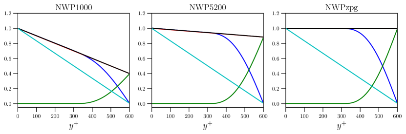
Figure 3: Blue: model total stress $\tau^{+}_{\text{model}}(y^{+})=\partial U^{+}/\partial y^{+}-\left\langle u^{\prime}v^{\prime}\right\rangle^{+}$; Red: target total stress $\tau_{\rm target}^{+}=1+y^{+}\,dP^{+}/dx^{+}$; Green: Primitive $F^{+}(y^{+})$ of forcing function $f^{+}$; Black: $\tau^{+}_{\text{model}}(y^{+})+F^{+}(y^{+})$; Cyan: total stress for a simulation without the forcing function $f^{+}$; for all the three model cases listed in table 1.

2.5 Computational parameters

The remaining model parameters, consistent for all simulation cases, are summarized in table 2. The size of the rectangular domain $\Omega$ is taken to be $L_{x}^{+}=L_{z}^{+}=1500$ and $L_{y}^{+}=600$; these values, while somewhat arbitrary, were determined through a combination of numerical experimentation and the spectral analysis of Lee & Moser (2019). Their work suggests that the contributions to the turbulent kinetic energy from modes with wavelengths $\lambda^{+}<1000$ are universal and $Re_{\tau}$-independent in a region below a wall-normal distance of approximately $y^{+}=300$. Accordingly, $L_{y}^{+}=2\cdot 300=600$ is chosen to allow for a sufficiently large fringe-region to mollify the effect of the nonphysical computational boundary at $y=L_{y}$ (see figure 2), and both $L_{x}^{+}$ and $L_{z}^{+}$ are taken to be at least 1000.

For the domain size in the stream/spanwise directions, there generally is a balance between computational cost and the accuracy of the model, as defined by a comparison of the model’s energy spectral density with that of large scale DNS. In particular, a variety of domain sizes were tested, ranging from $L_{x}^{+}=L_{z}^{+}=1000$ to approximately $3500$. Increasing $L_{x}$ and $L_{z}$ results in better agreement of the model’s low-wavenumber, large-scale portion of the energy spectral density with the corresponding portion computed from DNS. The high-wavenumber, small-scale portion of the model’s energy density, however, was insensitive to the domain size, so long as $L_{x}$ and $L_{z}$ were not taken to be too close to $L_{x}^{+}=L_{z}^{+}=1000$. In particular, $L_{x}^{+}=L_{z}^{+}=1500$ was found to be the smallest domain size capable of reproducing the universal small-scales discussed in section 3.3.

Given some target turbulent flux of mean momentum $\tau_{\rm turb}$, the auxiliary forcing $f$ must satisfy (2), but it is otherwise unconstrained. For the simulations reported here, $f$ is defined explicitly to be

$$f(y)=\begin{cases}\begin{array}[]{rr}4\tau_{\rm turb}/L_{y}^{4}\left(L_{y}-2y\right)^{2}\left(5L_{y}-4y\right),&y\in[L_{y}/2,L_{y}]\\ 0,&y\in[0,L_{y}/2],\end{array}\end{cases}$$ (11)

which was chosen to satisfy $f(L_{y}/2)=f^{\prime}(L_{y}/2)=f^{\prime}(L_{y})=0$. In particular the constraint $f^{\prime}(L_{y}/2)=0$ is important so that the transition in forcing from the near-wall region to the fringe region is smooth. Other functional forms of $f$, however, are of course possible. In particular a quadratic profile satisfying (2) and $f(L_{y}/2)=f^{\prime}(L_{y}/2)=0$ was tested, and no detectable changes in the statistics in the near-wall region $y^{+}\in[0,300]$ were found.

2.6 Numerical implementation and resolution

The model (1) is solved numerically using the velocity-vorticity formulation due to Kim et al. (1987). The equations of motion are discretized with a Fourier-Galerkin method in the stream/spanwise directions and a seventh order B-spline collocation method in the wall-normal direction (Kwok et al., 2001; Botella & Shariff, 2003; Lee & Moser, 2015). They are integrated in time with a low-storage, third order Runge-Kutta method that treats diffusive and convective terms implicitly and explicitly, respectively (Spalart et al., 1991). The numerical resolution in both space and time is consistent with that of DNS. The number of Fourier modes, and hence the numerical resolution, used in each simulation is listed in table 2, and can be compared with, for instance, table 1 in Lee & Moser (2015). In addition, the collocation point spacing in the wall-normal direction is similar to previous DNS studies; the total number of collocation points $N_{y}$ is taken to be equal to the number of collocation points below $y^{+}=600$ in Lee & Moser (2015). They are then distributed in the near wall region according to the same (shifted and rescaled) stretching function.

The model is implemented with a modified version of the PoongBack DNS code (Lee et al., 2013, 2014), and the initial condition is taken from a restart file from a DNS run that is truncated to fit in $\Omega$ at the resolutions listed in table 2 and modified to satisfy the boundary conditions 1.

$\psi^{+}$	$L_{x}^{+}=L_{z}^{+}$	$L_{y}^{+}$	$N_{x}$	$N_{z}$	$N_{y}$	$\Delta x^{+}$	$\Delta z^{+}$	$\Delta y^{+}_{w}$
00	15000	6000	120	256	192	12.50	5.860	0.0028170

Table 2: Summary of simulation parameters consistent for all simulation cases; $\psi$ is the prescribed value for the Neumann boundary condition in (1). $N_{x}$ and $N_{z}$ refer to the number of Fourier modes, while $N_{y}$ is the number of B-spline collocation points. $\Delta x=L_{x}/N_{x}$ and similarly for $\Delta z$. $\Delta y_{w}$ is the collocation point spacing at the wall.

2.7 Statistical convergence

The method of Oliver et al. (2014) is used to assess the uncertainty in the statistics reported due to sampling noise. For each pressure gradient case, statistics are collected by averaging in time until the estimated statistical uncertainty in the mean stress profiles is less than a few percent. For the cases in table 2 reported here, the sampling error is less than three percent, as shown in figure 4.

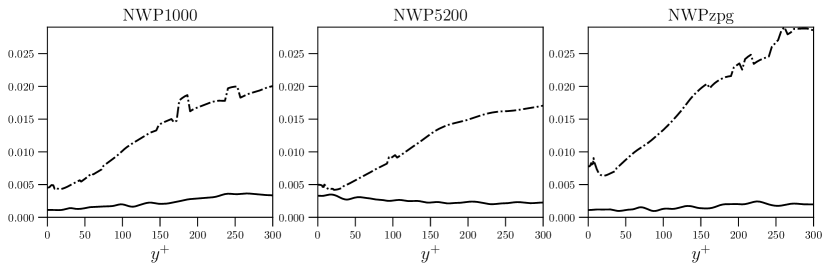
Figure 4: Statistical convergence for the model cases listed in table 2– solid lines: Absolute error $|\tau^{+}_{\text{model}}(y^{+})-\tau_{\rm target}(y^{+})|$, where $\tau^{+}_{\text{model}}=\partial U^{+}/\partial y^{+}-\left\langle u^{\prime}v^{\prime}\right\rangle^{+}$ and $\tau^{+}_{\rm target}=1+y^{+}dP^{+}/dx^{+}$; dash-dotted lines: Standard deviation of the estimated statistical error for $\tau^{+}_{\text{model}}$ in the region $y^{+}\in[0,300]$.

3 Numerical results

The near-wall patch model can be interpreted in two ways. In the first, one considers it to be a model for the small-scale near-wall turbulence in a wall bounded flow with mean pressure gradient in wall units the same as the imposed pressure gradient in the model. In this case, one aspires to have the statistics from the model and the real flow match for quantities that are insensitive to the unrepresented large scales or for the statistics of the small scales computed from a low-pass filter as in Lee & Moser (2019). This is the interpretation explored in the results reported here. In the second interpretation, the NWP model represents small-scale near-wall turbulence in a region of a real wall-bounded turbulent flow with local pressure gradient in wall units based on the local wall shear stress the same as that imposed in the model. In this case, the NWP model is analogous to the universal signal of Mathis et al. (2011), representing the process that is modulated by large-scale outer-layer fluctuations in a real turbulent flow. These interpretations are clearly complementary, and both should be valid given the scale-separation assumptions on which the model is predicated.

The statistics reported here were computed from the three near wall patch model cases NWP1000, NWP5200, and NWPzpg. The first two are so named because the imposed favorable pressure gradient in these cases is the same in wall units as the mean pressure gradient in a fully developed channel flow with friction Reynolds number $Re_{\tau}=1000$ and 5200. For NWPzpg, the imposed pressure gradient is zero. To assess the quality of the NWP, statistics from the model will be compared to those from the channel flow DNS of Lee & Moser (2015, 2019) at $Re_{\tau}=1000$ and $Re_{\tau}=5200$–referred to below as LM1000 and LM5200 (statistics at https://turbulence.ices.utexas.edu), and the zero pressure turbulent boundary layer DNS of Sillero et al. (2013); Borrell et al. (2013); Simens et al. (2009) at $Re_{\tau}=2000$, which is referred to below as SJM2000 (statistics at https://torroja.dmt.upm.es/turbdata/blayers/high_re/). So, comparisons are being made to flows in which the mean pressure gradient is the same in wall units as the imposed pressure gradient in the NWP models. However, many wall shear flows can have the same $\partial P^{+}/\partial x^{+}$. For example, the NWP1000 and NWP5200 cases could equally well be associated with favorable pressure gradient boundary layers and the NWPzpg case has imposed pressure gradient consistent with an infinite Reynolds number channel. Note that there is streamwise evolution of the mean wall shear stress in SJM2000, which is not the case in the channel flow cases. The comparison here is hence predicated on this evolution occurring over scales that are asymptotically large relative to the viscous scale, which indeed is the case.

3.1 Mean velocity and shear stresses

If the near-wall turbulence fluctuations represented in the NWP model dominate the Reynolds stress, as is expected from the spectral analysis of Lee & Moser (2019), then the mean velocity in the NWP should match that in a full turbulent flow. Figure 5 demonstrates that this is indeed the case. The relative error in $U^{+}$ is less than $0.6\%$ for $y^{+}\in[0,300]$, and the error is similarly small for the log-law indicator function $\beta^{+}$

$$\beta^{+}(y^{+}):=y^{+}\,\frac{\partial U^{+}}{\partial y^{+}}$$ (12)

in the range $y^{+}\in[0,100]$. However, there is mild disagreement of $\beta$ in the range $y^{+}\in[100,300]$. As expected, the profiles diverge for $y^{+}>300$.

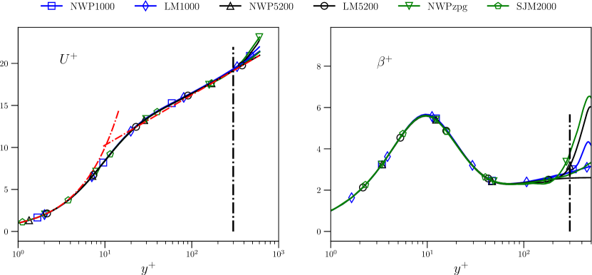
Figure 5: Mean velocity $U^{+}$ (left) and the indicator function $\beta^{+}=y^{+}\,\partial_{y^{+}}U^{+}$ (right) versus $\log(y^{+})$. The black dashed-dotted vertical line marks $y^{+}=300$, and the red dashed-dotted lines plot the law-of-the-wall $U^{+}=y^{+}$ and $U^{+}=(1/\kappa)\log(y^{+})+B$, where $\kappa=0.384$ and $B=4.27$ (Lee & Moser, 2015).

The NWP model’s Reynolds shear stress $\left\langle u^{\prime}v^{\prime}\right\rangle$ is in excellent agreement with that of the DNS in the region $y^{+}\in[0,300]$, as expected given the agreement of the mean velocity; see figure 6. For the channel cases, the error is less than $0.5\%$, and for the zero pressure gradient case the error is below $4\%$. In the former, the total stress at $y=L_{y}$ is known analytically as $\tau^{+}_{\rm tot}=1+L_{y}^{+}dP^{+}/dx^{+}$ and is used to define $f(y)$ in (2), (8), and (9). In the latter, the same relations are used, though they are approximate due to the streamwise growth of the near wall layer in a boundary layer. This may explain the relatively larger discrepancy between the $\left\langle u^{\prime}v^{\prime}\right\rangle$ profiles for the boundary layer. In both instances, recall that $\left\langle u^{\prime}v^{\prime}\right\rangle$ necessarily vanishes at the upper computational boundary as a consequence of the boundary condition $v=0$ in (1). The accuracy of the Reynolds shear stress profiles in spite of this condition demonstrates the utility of the forcing function $f$ in enabling momentum transport to the near wall region $y^{+}\in[0,300]$.

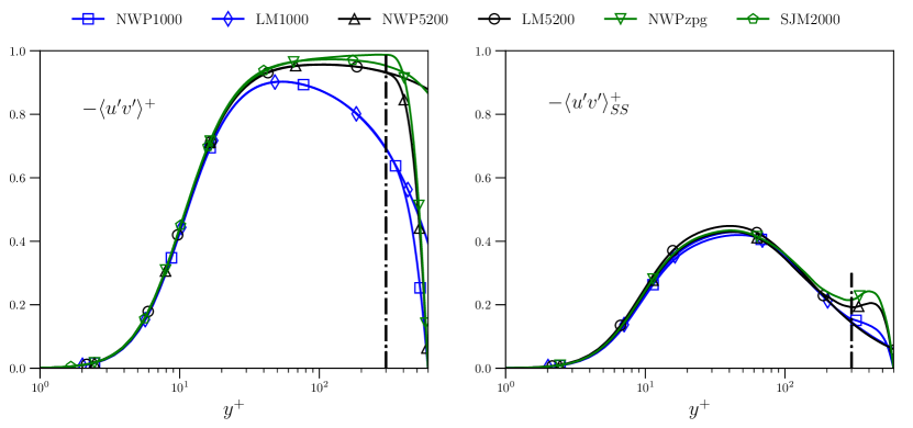
Figure 6: (a) Reynolds stress $-\left\langle u^{\prime}v^{\prime}\right\rangle^{+}$ and (b) the filtered Reynolds stress $-\left\langle u^{\prime}v^{\prime}\right\rangle^{+}_{SS}$ (defined by (19) and discussed in section 3.3) as a function of $\log(y^{+})$. The black dashed-dotted vertical line marks $y^{+}=300$.

3.2 Energy spectral density

For two points $(x,y,z),(x^{\prime},y,z^{\prime})\in\mathbb{R}\times[0,2\delta]\times\mathbb{R}$ in an infinitely long channel, define the separation distances $r_{x}=x-x^{\prime}$ and $r_{z}=z-z^{\prime}$. For a turbulent flow that is statistically homogeneous in the stream and spanwise directions, the two point correlation tensor

$$R_{ij}(r_{x},y,r_{z}):=\left\langle u_{i}^{\prime}(x+r_{x},y,z+r_{z})u_{j}^{\prime}(x,y,z)\right\rangle$$ (13)

is a function only of $r_{x}$, $y$, and $r_{z}$. Taking the Fourier transform of (13) in the variables $r_{x}$ and $r_{z}$ defines the spectral density $E_{ij}(k_{x},y,k_{z})$, which encodes the average contribution to the Reynolds stress tensor from different length scales as a function of the wall-normal variable $y$. The Reynolds stress tensor can be recovered by taking the limit $(r_{x},r_{z})\to(0,0)$ in (13), or by integrating the spectral density over all wavenumbers

$$\left\langle u_{i}^{\prime}u_{j}^{\prime}\right\rangle(y)=\int\int E_{ij}(k_{x},y,k_{z})dk_{x}\,dk_{z}.$$ (14)

For a wall bounded flow in a full size domain, the low-wavenumber contributions to the Reynolds stress represent the mean influences of the large scale structures on the near wall dynamics. As is well known (Hutchins & Marusic, 2007; Marusic et al., 2010a; Lee & Moser, 2017; Samie et al., 2018; Lee & Moser, 2019), these low-wavenumber features of the near wall flow depend on $Re_{\tau}$. In contrast, there is evidence that the high-wavenumber (small-scale) contributions to the Reynolds stress profiles are universal and independent of $Re_{\tau}$ (Samie et al., 2018; Lee & Moser, 2019). By design, the NWP model’s domain size does not allow accurate representation of the very large-scale structures known to exist in the near wall region, and thus one cannot expect to capture their influence on the near-wall velocity fluctuations. Instead, one expects the NWP model to correctly capture the dynamics of the universal small scales elucidated by Samie et al. (2018) and Lee & Moser (2019) associated with the autonomous cycle of Jiménez & Pinelli (1999).

To determine whether or not this is the case, the model’s spectra $E_{ij}$ are compared to their DNS counterparts. The spectra are visualized in so-called log-polar coordinates (Lee & Moser, 2019), in which the wavenumber magnitude $k=\sqrt{k_{x}^{2}+k_{z}^{2}}$ is represented on a logarithmic scale. For fixed wall-normal location, the log-polar coordinates are defined as

$$k_{x}^{\#}:=\frac{k_{x}}{k}\log_{10}\left(\frac{k}{k_{\text{ref}}}\right)$$ (15)

$$k_{z}^{\#}:=\frac{k_{z}}{k}\log_{10}\left(\frac{k}{k_{\text{ref}}}\right)$$

where $k_{\text{ref}}$ is an arbitrary reference wavenumber that must be smaller than the smallest nonzero wavenumber included in the spectrum, taken here to be $k^{+}_{\text{ref}}=1/50\,000$. Two advantages of these coordinates are that lines of constant $k_{z}/k_{x}$ have slopes of $k_{z}/k_{x}$, and lines of constant magnitude $k$ map to circles. In this way, the orientation and alignments of the Fourier modes are easily interpreted; see Lee & Moser (2019) for a more detailed discussion.

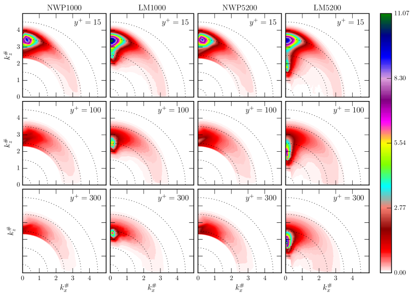
Figure 7: Two-dimensional spectra of the streamwise velocity variance $\left\langle u^{\prime}u^{\prime}\right\rangle^{+}$ in log-polar coordinates, as defined by equation (15). $\lambda^{+}=10$ on the outermost dotted circle and increases by a factor of 10 for each dotted circle moving inward, where $\lambda=2\pi/k$ is the wavelength.

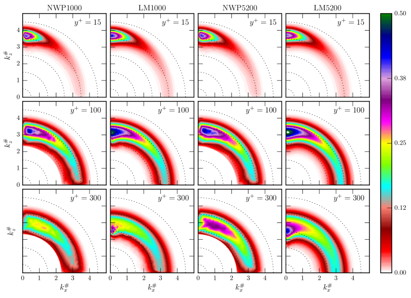
Figure 8: Two-dimensional spectra of the wall-normal velocity variance $\left\langle v^{\prime}v^{\prime}\right\rangle^{+}$ in log-polar coordinates, as defined by equation (15). $\lambda^{+}=10$ on the outermost dotted circle and increases by a factor of 10 for each dotted circle moving inward, where $\lambda=2\pi/k$ is the wavelength.

The two-dimensional spectral densities of the streamwise and wall-normal velocity variances are shown in figures 7 and 8, respectively. The spectra are visualized at the wall-normal locations $y^{+}=15$, $y^{+}=100$ and $y^{+}=300$ for the simulations NWP1000, NWP5200, LM1000, and LM5200.

In each of the cases, the streamwise velocity spectra $E_{11}$ consist primarily of energy concentrated along the $k_{z}^{\#}$ axis, with Fourier modes for which $k_{z}/k_{x}\gtrsim 10$ (Lee & Moser, 2019). These correspond to structures that are strongly elongated in the streamwise $x$-direction, such as the well-known, near wall low and high speed streaks. The channel flow data LM1000 and LM5200 (columns two and four in figure 7) show that this energy exhibits two distinct features. The first is an “inner energy site” (Samie et al., 2018), a triangular shaped region in the near wall layer $y^{+}\approx 15$ distributed primarily between wavelengths $\lambda^{+}=100$ and $\lambda^{+}=1000$ that can be attributed to the autonomous near wall dynamics described by Hamilton et al. (1995); Jeong et al. (1997); Jiménez & Pinelli (1999), and others. The model $E_{11}$ spectra, shown in columns one and three in figure 7, qualitatively reproduce the inner energy site, suggesting that it captures the dynamics of the near wall, small scale energetic motions.

The second feature is a concentration of energy at relatively low wavenumbers (in the range $1000<\lambda^{+}<10\,000$) along the $k_{z}^{\#}$ axis at each of the wall-normal locations $y^{+}=15$, $y^{+}=100$, and $y^{+}=300$. These are due to the very large scale motions (VLSMs) imposed from the outer layer flow described by Hutchins & Marusic (2007) and Marusic et al. (2010a). These VLSMs contribute energy in the near wall region around $y^{+}=15$, and farther away from the wall they are responsible for the majority of the turbulent kinetic energy. As both $y^{+}$ and $Re_{\tau}$ increase, the energy becomes more concentrated and is found at larger wavelengths, consistent with the attached eddy hypothesis of Townsend (1976). In addition, the VLSMs modulate the near wall cycle through nonlinear interactions, creating large scale variations in the local wall shear stress that result in local variations in the dominant (most-energetic) wavelength (Lee & Moser, 2019). Consequently, the spectral peak of the inner energy site for the DNS data is reduced and “smeared out” as a function of $Re_{\tau}$. For example, the $Re_{\tau}=5200$ peak is about ten percent lower than the $Re_{\tau}=1000$ peak.

By design, the NWP model can only support modes with wavelengths less than or equal to $L_{x}^{+}=L_{z}^{+}=1500$, meaning the VLSMs present in real wall bounded turbulence are not represented by the model. As a result, there is no energy associated with such large scale structures; the concentration of energy at low wavenumbers along the $k_{z}^{\#}$ axis (corresponding to wavelengths $\lambda^{+}\gtrsim 1000$) present in the DNS spectra is not present in that of the model. This is true both in the near wall region and farther away from the wall at $y^{+}=100$ and $y^{+}=300$.

Furthermore, the NWP model does not capture the nonlinear modulations of the autonomous cycle by the VLSMs. For instance, even though the model represents wavenumbers along the $\lambda^{+}=1000$ band, its spectra is not simply a spectral truncation of the DNS spectra. Additionally, the peak of the inner energy site is nearly identical for the two model cases, differing by only a few percent. These differences between spectra of the model and DNS highlight the important role the VLSMs play in the turbulent near wall layer.

The $E_{22}$ spectra are largest in the wavenumber regions in which the $E_{11}$ spectra are peaked, as discussed in Lee & Moser (2019). Additionally, the distribution of energy generally becomes more isotropic with increasing wall-normal distance $y^{+}$. Figure 8 shows that the DNS energy density $E_{22}$ is primarily, but not exclusively, located at the small scales, i. e. at wavenumbers $\lambda^{+}<1000$. Because the NWP model adequately resolves such structures, its energy density $E_{22}$ is in overall good agreement with the DNS spectra, especially in the near wall region. Farther away from the wall the agreement is not as good since the DNS spectra are peaked at lower wavenumbers. Accordingly, the model’s unfiltered $\left\langle v^{\prime}v^{\prime}\right\rangle$ profiles shown in figure 10 show excellent agreement with the corresponding DNS profiles in region $y^{+}\in[0,300]$; they are nearly identical for $y^{+}\lesssim 50$ and only display slight discrepancies for $y^{+}\in[50,300]$.

Lastly, fidelity of the NWP model’s energy density $E_{33}$ (not shown) in reproducing the DNS spectra is similar to the $E_{11}$ spectra. It clearly approximates the small scales in the near wall region well, but it fails to capture the modulation by the large scale structures at each wall-normal location.

3.3 Universality of small scales

To better quantify the universality of the small scales and assess the NWP model’s ability to reproduce them, the energy spectral density is high-pass filtered and then integrated to measure the energy residing in the small scales. Let $\mathcal{K}$ denote the set of wavenumbers supported by a simulation, and let $k_{\rm cut}=2\pi/\lambda_{\rm cut}$ with $\lambda^{+}_{\rm cut}=1000$. Define $\mathcal{K}_{SS}$ to be the subset of $\mathcal{K}$ with the property that $(k_{x},k_{z})\in\mathcal{K}_{SS}$ if

$$\min\{|k_{x}|,|k_{z}|\}>k_{\rm cut},$$ (16)

visualized in figure 9 (left). The $\mathcal{K}_{SS}$ sets are meant to contain large wavenumbers associated with the universal small scales. Here $k_{\rm cut}$ is chosen based on the two-dimensional spectra in Lee & Moser (2019), where it is observed that the energy associated with the autonomous cycle has $\lambda^{+}<1000$.

Note the high-pass filter (16) is slightly different than the $L^{2}$ filter

$$\sqrt{k_{x}^{2}+k_{z}^{2}}>k_{\rm cut}$$ (17)

used in Lee & Moser (2019) and visualized in figure 9 (right). In particular, the wavenumbers on the axis $k_{x}=0$ (respectively $k_{z}=0$) with $k_{z}>k_{\rm cut}$ (resp. $k_{x}>k_{\rm cut}$) are filtered out by (16) but not by (17). These axes contain the NWP model’s approximation to the large scale motions present in a DNS that do not “fit” in the near wall patch domain. Such motions correspond to wavenumbers smaller than $2\pi/L_{x}=2\pi/L_{z}$, and they are not well represented by the NWP model. Hence, they are filtered out by (16). The approximation can be improved by increasing $L_{x}$ and $L_{z}$ (confirmed by numerical tests), although this of course increases the model’s overall computational cost.

Figure 9: (Left) The shaded gray region indicates the subset (in the first quadrant) of wavespace $\mathcal{K}_{SS}$ defined by (16). (Right) the corresponding region defined instead by the circular, $L^{2}$ filter (17) used in Lee & Moser (2019).

Given $\mathcal{K}$ and $\mathcal{K}_{SS}$, the Reynolds stresses are

$$\left\langle u_{i}^{\prime}u_{j}^{\prime}\right\rangle(y)=\sum_{(k_{x},k_{z})\in\mathcal{K}}E_{ij}(k_{x},y,k_{z}),$$ (18)

and the small scale energy can be quantified as

$$\left\langle u_{i}^{\prime}u_{j}^{\prime}\right\rangle_{SS}(y)=\sum_{(k_{x},k_{z})\in\mathcal{K}_{SS}}E_{ij}(k_{x},y,k_{z}).$$ (19)

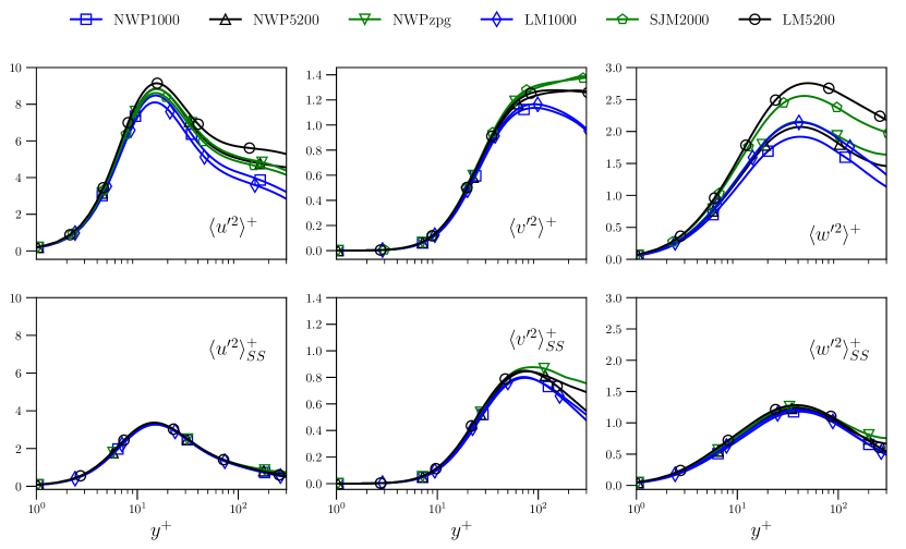
Figure 10: Velocity variances $\left\langle u^{\prime}_{\alpha}u^{\prime}_{\alpha}\right\rangle^{+}$ (top) and the corresponding high-pass filtered quantities $\left\langle u^{\prime}_{\alpha}u^{\prime}_{\alpha}\right\rangle^{+}_{SS}$ (bottom) as a function of $\log(y^{+})$.

The velocity covariance $\left\langle u^{\prime}v^{\prime}\right\rangle$ and variances $\left\langle u^{\prime}_{\alpha}u^{\prime}_{\alpha}\right\rangle$, $\alpha=1,2,3$ and their high-pass filtered counterparts are shown in figures 6 and 10, respectively. As previously mentioned, the model’s unfiltered $\left\langle u^{\prime}v^{\prime}\right\rangle$ and $\left\langle v^{\prime}v^{\prime}\right\rangle$ profiles both agree quite well with the corresponding DNS profiles. The model’s streamwise and spanwise velocity variances, however, display nontrival discrepancies with the DNS profiles, as expected from the observed differences in the two dimensional spectra. In contrast, the model’s high-pass filtered profiles all show agreement with the high-pass filtered DNS quantities. In all cases the agreement is excellent in the region $y^{+}\in[0,100]$, although there are some relatively mild discrepancies for $y^{+}\in[100,300]$. Moreover, it is clear that the high-pass filtered quantities are nearly $Re_{\tau}$ independent; the collapse of the $\left\langle u^{\prime}u^{\prime}\right\rangle_{SS}$ profiles is particularly convincing. Although two-dimensional spectra data is not available for the zero-pressure gradient DNS case SJM2000, the $\left\langle u_{i}^{\prime}u_{j}^{\prime}\right\rangle_{SS}$ profiles computed from the model simulation NWPzpg are included for completeness; they display the same universal behavior as the favorable pressure gradient flows. These observations lend support to the conclusion that the small scales in the near wall region are universal, and that the difference in the Reynolds stress profiles as a function of $Re_{\tau}$ is due to the increasing influence of the VLSMs. Previous results of this type obtained in both Lee & Moser (2019) and Samie et al. (2018) involve high-pass filtering the entire turbulent flow field, in which there are nonlinear interactions between wavenumbers across all the scales of motion. It is particularly remarkable, however, that the NWP model reproduces the universal behavior of the small scales without the dynamic modulation of the near wall autonomous cycle by the large scale structures.

3.4 Reynolds Stress Transport

The production of turbulent kinetic energy in a wall bounded flow is primarily due to the large mean velocity gradient in the wall normal direction $\partial U/\partial y$. In a flow that is homogeneous in the stream/spanwise directions with $V=W=0$, the only $\left\langle u^{\prime}_{\alpha}u^{\prime}_{\alpha}\right\rangle$ term with a nonzero production is $\left\langle u^{\prime}u^{\prime}\right\rangle$; it is given by

$$\mathcal{P}_{11}=-2\,\frac{\partial U}{\partial y}\,\left\langle u^{\prime}v^{\prime}\right\rangle.$$ (20)

The two dimensional spectra of $\mathcal{P}_{11}$ is accordingly defined as

$$E_{11}^{\mathcal{P}}(k_{x},y,k_{z}):=-2\,\frac{\partial U}{\partial y}(y)\,E_{12}(k_{x},y,k_{z}).$$ (21)

The spectral analysis of channel flow data in Lee & Moser (2019) demonstrated that in contrast to the near wall energy spectra $E_{11}$, the near wall production spectra $E^{\mathcal{P}}_{11}$ contains only a high wavenumber peak (see columns two and four in figure 11). It follows that the large scales in the near wall region, and hence the energy that they contain, are due to energy transport (either in $y$ or in scale), rather than local production. This observation suggests that the NWP model should be able to capture the near wall energy production, even though the VLSMs are not present. The production spectra shown in figure 11 show that this is indeed true. At both $y^{+}=15$ and $y^{+}=30$, the NWP1000 and NWP5200 spectra are qualitatively similar to that of DNS, including the regions of negative production occurring over a range of scales around $\lambda^{+}=100$. Farther away from the wall, the large scale structures increasingly influence the energy production, and their influence increases with $Re_{\tau}$. At $y^{+}=300$, the large scale influences dominate the DNS production spectra, and the model is not able to reproduce such low wavenumber features.

The one-dimensional, premultiplied production profiles are shown in figure 12, and they are consistent with the aforementioned observations regarding the two-dimensional spectra. The DNS profiles are approximately $Re_{\tau}$-independent for $y^{+}\lesssim 70$, the corresponding model profiles show strong agreement for $y^{+}\lesssim 100$, and they begin to show modest discrepancies for $y^{+}\gtrsim 200$.

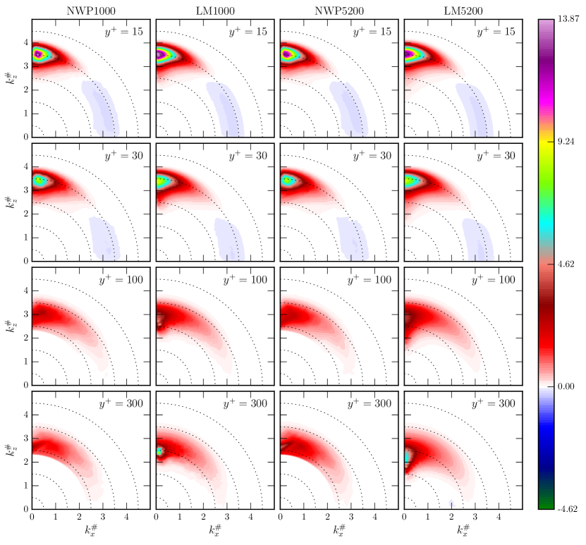
Figure 11: Two-dimensional, premultiplied spectra $y^{+}\,(E^{\mathcal{P}}_{11})^{+}$ in log-polar coordinates, as defined by equation (15). $\lambda^{+}=10$ on the outermost dotted circle and increases by a factor of 10 for each dotted circle moving inward, where $\lambda=2\pi/k$ is the wavelength.

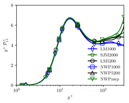
Figure 12: Profiles of the premultiplied $\left\langle u^{\prime}u^{\prime}\right\rangle$ production $\mathcal{P}^{+}_{11}$ versus $\log(y^{+})$ in the region $y^{+}\in[0,300]$.

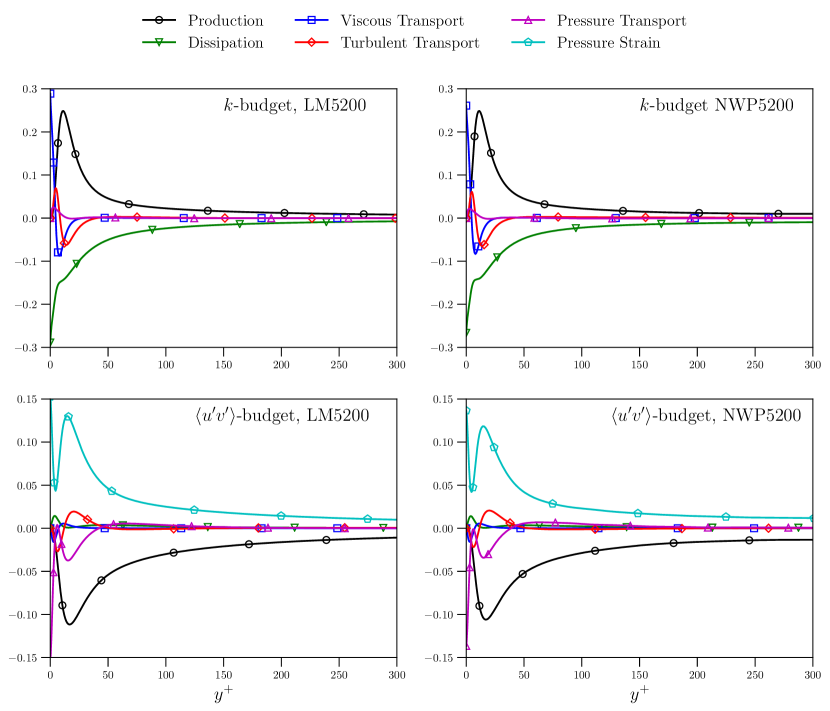
Figure 13: Budget equations of the turbulent kinetic energy $k=\left\langle u_{i}^{\prime}u_{i}^{\prime}\right\rangle/2$ (top) and shear stress $\left\langle u^{\prime}v^{\prime}\right\rangle$ for the largest Reynolds number cases LM5200 (left) and NWP5200 (right). The terms are defined in the appendix (22)

After being produced by the mean velocity gradient, turbulent kinetic energy is redistributed across scales and velocity components, transported both towards and away from the wall, and ultimately dissipated by viscosity. The relative strength, or importance, of these processes as a function of wall-normal distance can be measured by the terms in the Reynolds stress budget equation (Pope, 2000). Exhaustive analyses of the behavior of these terms for wall bounded flows can be found in Hoyas & Jiménez (2008); Richter (2015); Mizuno (2015, 2016); Aulery et al. (2017); Lee & Moser (2019), and other references therein. A general conclusion to be drawn from these works is that, similar to the production and velocity variances, the small scale contributions to the terms in the budget equation are universal in the near wall region, and differences in the profiles as a function of $Re_{\tau}$ can be attributed to modulations by large scale motions.

As a consequence, the terms in the Reynolds stress budget equations evaluated in the NWP model are consistent with those in near-wall turbulence. For example, the terms in the turbulent kinetic energy and Reynolds shear stress budget equations are shown in figure 13 for both NWP5200 and LM5200. The precise definitions of the terms in figure 13 are standard, but for clarity they are specified in the appendix (22).

3.5 Near-wall Turbulence Structure

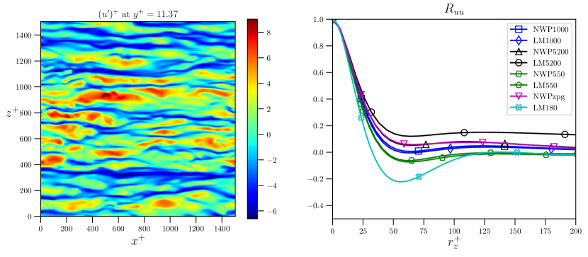
Figure 14: Left: snapshot of the streamwise velocity fluctuation $u^{\prime}$ in the $x-z$ plane; right: two-point correlation function $R_{uu}(r_{z})$ for all three model cases, as well as an additional model case NWP550, and channel flow DNS ranging from $Re_{\tau}\approx 180-5200$. Each $R_{uu}$ is measured at $y^{+}\approx 11.5$.

In addition to producing consistent near-wall statistics, the NWP model flow produces flow structures that are consistent with expectations for near-wall turbulence. For example, the well-known high- and low-speed streaks are apparent in visualizations of the streamwise velocity fluctuations near the wall (figure 14), and those streaks have the expected spanwise spacing, as evidenced by the two-dimensional spectra in figure 7 at $y^{+}=15$, and the spanwise two-point correlations of streamwise velocity fluctuations in figure 14. In the NWP flows, increasing the magnitude of the imposed favorable pressure gradient appears to increase the coherence of the streaks, as indicated by the depth of the mild local minimum at $r_{z}^{+}\approx 50$, though the imposed pressure gradient in the NWP5200 case is weak enough to have no effect relative to NWPzpg. The correlations from NWP1000 and NWP550 are also in excellent agreement with those of their corresponding channel flow DNS, while the correlations from NWP5200 and LM5200 are quite different. This is almost certainly due to the large scale modulations of the near wall turbulence that occurs in the high Reynolds number channel flow. This is apparent from the two-dimensional spectrum for LM5200 at $y^{+}=15$ (see figure 7), which cannot be represented in the NWP model, and which are largely absent in the lower Reynolds number channel flows (LM1000 at $y^{+}=15$ in figure 7).

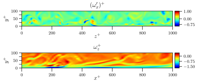
Figure 15: Contour plots of the streamwise vorticity fluctuation $\omega_{x}^{\prime}$ in the $y-z$ plane and spanwise vorticity $\omega_{z}$ in the $x-y$ plane.

In the autonomous near wall dynamics, the near wall streaks are formed by near wall streamwise vortices (Jiménez & Pinelli, 1999), and such streamwise vortices are indeed present in the NWP flow (figure 15). The presence of near wall streamwise vortices is also imprinted in the streamwise vorticity variance profiles (figure 16) in the local maximum that occurs at about $y^{+}=15$. Streamwise, wall-normal and spanwise vorticity variances in the NWP model flows are also all largely consistent with those from the channel flow and boundary layer DNS. Other features of the autonomous near wall dynamics include the predominantly streamwise vortices that lift up from the wall forming inclined vortices, as well as sharp gradients in the streamwise velocity that are manifested as inclined spanwise vorticity structures. These too are apparant in visualizations of spanwise vorticity from the NWP flows (figure 15).

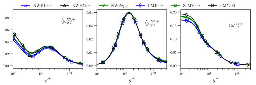
Figure 16: Vorticity variances $\left\langle\omega^{\prime}_{\alpha}\omega^{\prime}_{\alpha}\right\rangle^{+}$ versus $\log(y^{+})$ in the region $y^{+}\in[0,300]$.

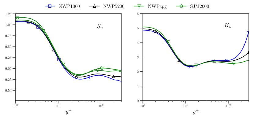
Figure 17: Skewness $S_{u}$ and kurtosis $K_{u}$ of the streamwise velocity fluctuations in the NWP cases, and skewness in SJM2000.

Given the consistency of the NWP flow structures with those of near-wall turbulence, one would expect that higher order statistical quantities would also be consistent. As an example, the skewness and kurtosis of the streamwise velocity fluctuations are shown in figure 17. While these quantities are not as widely reported, and are in particular not currently available for LM1000 and LM5200, their profiles in the NWP cases are none-the-less consistent with data in the literature (Monty et al., 2009; Chin et al., 2015; Samie et al., 2018). In particular, skewness has a local minimum at $y^{+}\approx 20$, crosses zero at $y^{+}\approx 10$ and attains a maximum at the wall of about 1.1. Also, kurtosis has a local minimum at $y^{+}\approx 10$ and reaches a maximum at the wall of about 5.

4 Conclusions

The near-wall patch (NWP) model of near-wall turbulence described here was formulated in part to address the hypothesis that the autonomous dynamics of the near-wall turbulence modulated by the large-scale outer-layer turbulence is responsible for the observed characteristics of near-wall turbulence. The NWP flow was also formulated to serve as as a computationally accessible quantitative model of near-wall turbulence which will be useful in a number of contexts.

Regarding the former objective, the study described here builds on previous work by Jiménez & Pinelli (1999) and Jiménez & Moin (1991), which use simulations with restricted periodic domains, and in the case of Jiménez & Pinelli (1999), manipulation of the turbulence outside the near wall layer. These simulations were used to characterize in detail the fluid dynamic processes responsible for near-wall turbulence, and establish that these processes are autonomous, not requiring interaction with the outer turbulence. Here, however, the objectives were different, and so the domain sizes, while still restricted, are larger in the horizontal and vertical directions (1500 and 600 wall units, respectively), motivated by the spectral analysis of Lee & Moser (2019)).

The statistical profiles from the NWP flows are in close agreement with those from DNS of turbulent channels and a boundary layer in large spatial domains. For some quantities for which very large scales make a significant contribution, such as the streamwsie velocity variance, this agreement is attained only after the large-scale fluctuations that are too large to be represented in the NWP have been filtered out. This indicates that there is a universal near-wall small-scale dynamics that produces the familiar statistics of near-wall turbulence, which had been suggested previously based on analysis of both experimental and DNS data from wall bounded turbulent flows (Marusic et al., 2010b; Mathis et al., 2011; Lee & Moser, 2019). By actually simulating the autonomous near-wall dynamics over the range of scales at which they occur, as determined from spectral analysis (Lee & Moser, 2019), we confirm that the “universal signal” described by Marusic et al. (2010b); Mathis et al. (2011) arises from universal dynamics, where universal here means independent of Reynolds number or external flow configuration.

As a quantitative model of near-wall turbulence, the NWP flow defines a one-dimensional family of near-wall turbulent flows, parameterized by the imposed streamwise pressure gradient $\partial P^{+}/\partial x^{+}$. In this context, the NWP model can, for example, be used as a source of data to inform a wall model for wall-modeled large eddy simulation (LES). For such an application, one would invoke the scale separation assumption discussed in §2.2 and use NWP flows matched to the local pressure gradient and momentum flux associated with the large-scale outer-layer flow simulated by the LES. Other applications of the NWP model are as a vehicle for numerical experiments on near wall turbulence as in Jiménez & Pinelli (1999) and to investigate the interactions of the small-scale, near wall turbulence with such complications as surface roughness, heat transfer, chemical reactions, and turbophoresis. These applications of the NWP were out of scope for the current study, but the NWP model allows such near wall phenomena to be studied computationally at a much lower cost than a full DNS of a real turbulent flow. For example, the NWP computational grid is a factor of 24080 smaller than the DNS grid used for the LM5200 channel case.

Finally, the NWP formulation described here can be considered a lowest order asymptotic description of near-wall turbulence, in which the imposed pressure gradient, the momentum flux from the outer flow and the mean wall shear stress are considered uniform in space and time on the scale of the patch. A higher order approximation could allow one or more of these quantities to vary slowly in the streamwise direction or time, which can be treated asymptotically as in Spalart (1988) or Topalian et al. (2017) to model the resulting spatial or temporal evolution of the wall turbulence. This would broaden the applicability of NWP models, which, for example, would allow them to be used with stronger pressure gradients, especially strong adverse pressure gradient boundary layers in which wall shear stress generally evolves relatively rapidly.

5 Acknowledgments

The work presented here was supported by the National Science Foundation Award no. (DMS-1620396), as well as by the Oden Institute for Computational Science and Engineering. The research utilized the computing resources of the Texas Advanced Computing Center (TACC) at the University of Texas at Austin.

We wish to thank Myoungkyu Lee for assistance with the PoongBack code, supplying post-processing scripts for visualizing data, and insightful discussions. We also thank Todd Oliver, Prakash Mohan, and Gopal Yalla for insightful discussions and useful suggestions for this manuscript.

The authors report no conflicts of interest.

Appendix A Reynolds stress budget equation

The Reynolds stress budget equations govern the evolution of the Reynolds stress tensor. The terms of the equation are given by:

$$\frac{D\left\langle u_{i}^{\prime}u_{j}^{\prime}\right\rangle}{Dt}= -\overbrace{\left(\left\langle u_{i}^{\prime}u_{k}^{\prime}\right\rangle\frac{\partial U_{j}}{\partial x_{k}}+\left\langle u_{j}^{\prime}u_{k}^{\prime}\right\rangle\frac{\partial U_{i}}{\partial x_{k}}\right)}^{\mathcal{P}_{ij}}$$ (22)

$$-\overbrace{\frac{\partial\left\langle u_{i}^{\prime}u_{j}^{\prime}u_{k}^{\prime}\right\rangle}{\partial x_{k}}}^{T_{ij}}+\overbrace{\nu\frac{\partial^{2}\left\langle u_{i}^{\prime}u_{j}^{\prime}\right\rangle}{\partial x_{k}\partial x_{k}}}^{D_{ij}}$$

$$+\overbrace{\left\langle p^{\prime}\left(\frac{\partial u_{i}^{\prime}}{\partial x_{j}}+\frac{\partial u_{j}^{\prime}}{\partial x_{i}}\right)\right\rangle}^{\Pi_{ij}}-\overbrace{\left(\frac{\partial\left\langle p^{\prime}u_{i}^{\prime}\right\rangle}{\partial x_{j}}+\frac{\partial\left\langle p^{\prime}u_{j}^{\prime}\right\rangle}{\partial x_{i}}\right)}^{\Upsilon_{ij}}$$

$$-\overbrace{2\nu\left\langle\frac{\partial u_{i}^{\prime}}{\partial x_{k}}\frac{\partial u_{j}^{\prime}}{\partial x_{k}}\right\rangle}^{\epsilon_{ij}}.$$

Here $\mathcal{P}_{ij}$ denotes turbulence production, $T_{ij}$ turbulent transport, $D_{ij}$ viscous transport, $\Pi_{ij}$ pressure strain, $\Upsilon_{ij}$ pressure transport, and $\epsilon_{ij}$ dissipation.

References

- Abdulle et al. (2012) Abdulle, A., E, W., Engquist, B. & Vanden-Eijnden, E. 2012 The heterogeneous multiscale method. Acta Numerica 21, 1–87.
- Aulery et al. (2017) Aulery, F., Dupuy, D., Toutant, A., Bataille, F. & Zhou, Y. 2017 Spectral analysis of turbulence in anisothermal channel flows. Computers & Fluids 151, 115 – 131.
- Berendsen et al. (1984) Berendsen, H. J. C., Postma, J. P. M., van Gunsteren, W. F., DiNola, A. & Haak, J. R. 1984 Molecular dynamics with coupling to an external bath. The Journal of Chemical Physics 81 (8), 3684–3690.
- Berselli et al. (2006) Berselli, L.C., Iliescu, T. & Layton, W.J. 2006 Mathematics of Large Eddy Simulation of Turbulent Flows. Springer.
- Borrell et al. (2013) Borrell, G., Sillero, J. A. & Jiménez, J. 2013 A code for direct numerical simulation of turbulent boundary layers at high Reynolds numbers in BG/P supercomputers. Computers and Fluids 80, 37–43.
- Bose & Park (2018) Bose, S. T. & Park, G. I. 2018 Wall-modeled large-eddy simulation for complex turbulent flows. Annual Review of Fluid Mechanics 50 (1), 535–561.
- Botella & Shariff (2003) Botella, O. & Shariff, K. 2003 B-spline Methods in Fluid Dynamics. International Journal of Computational Fluid Dynamics 17 (2), 133–149.
- Chin et al. (2015) Chin, C., Ng, H. C. H., Blackburn, H. M., Monty, J. P. & Ooi, A. 2015 Turbulent pipe flow at : A comparison of wall-resolved large-eddy simulation, direct numerical simulation and hot-wire experiment. Computers & Fluids 122, 26–33.
- Coleman et al. (2015) Coleman, G. N., Garbaruk, A. & Spalart, P. R. 2015 Direct numerical simulation, theories and modelling of wall turbulence with a range of pressure gradients. Flow, Turbulence and Combustion 95 (2), 261–276.
- Colonius (2004) Colonius, T. 2004 Modeling artificial boundary conditions for compressible flow. Annual Review of Fluid Mechanics 36, 315–345.
- Darcy (1854) Darcy, H. 1854 Recherches expérimentales rélatives au mouvement de l’eau dans les tuyeaux. Mém. Savants Etrang. Acad. Sci. Paris 17, 1–268.
- DeGraaff & Eaton (2000) DeGraaff, D. B. & Eaton, J. K. 2000 Reynolds-number scaling of the flat-plate turbulent boundary layer. Journal of Fluid Mechanics 422, 319–346.
- Ganapathisubramani et al. (2012) Ganapathisubramani, B., Hutchins, N., Monty, J. P., Chung, D. & Marusic, I. 2012 Amplitude and frequency modulation in wall turbulence. Journal of Fluid Mechanics 712, 61–91.
- Hagen (1839) Hagen, G. H. L. 1839 Über den bewegung des wassers in engen cylindrischen röhren. Poggendorfs Ann. Phys. Chem. 46, 423–42.
- Hamilton et al. (1995) Hamilton, J. M., Kim, J. & Waleffe, F. 1995 Regeneration mechanisms of near-wall turbulence structures. Journal of Fluid Mechanics 287, 317–348.
- Hoyas & Jiménez (2008) Hoyas, S. & Jiménez, J. 2008 Reynolds number effects on the Reynolds-stress budgets in turbulent channels. Physics of Fluids 20, 101511.
- Hutchins & Marusic (2007) Hutchins, N. & Marusic, I. 2007 Large-scale influences in near-wall turbulence. Philosophical Transactions of the Royal Society A: Mathematical, Physical and Engineering Sciences 365, 647–664.
- Jeong et al. (1997) Jeong, J., Hussain, F., Schoppa, W. & Kim, J. 1997 Coherent structures near the wall in a turbulent channel flow. Journal of Fluid Mechanics 332, 185–214.
- Jiménez & Moin (1991) Jiménez, J. & Moin, P. 1991 The minimal flow unit in near-wall turbulence. Journal of Fluid Mechanics 225, 213–240.
- Jiménez & Pinelli (1999) Jiménez, J. & Pinelli, A. 1999 The autonomous cycle of near-wall turbulence. Journal of Fluid Mechanics 389, 335–359.
- Khujadze & Oberlack (2004) Khujadze, G. & Oberlack, M. 2004 DNS and scaling laws from new symmetry groups of ZPG turbulent boundary layer flow. Theoretical Computational Fluid Dynamics 18, 391–411.
- Kim et al. (1987) Kim, J., Moin, P. & Moser, R. 1987 Turbulence statistics in fully developed channel flow at low Reynolds number. Journal of Fluid Mechanics 177, 133–166.
- Kwok et al. (2001) Kwok, W. Y., Moser, R. D. & Jiménez, J. 2001 A critical evaluation of the resolution properties of b-spline and compact finite difference methods. Journal of Computational Physics 174 (2), 510 – 551.
- Lee et al. (2013) Lee, M., Malaya, N. & Moser, R. D. 2013 Petascale direct numerical simulation of turbulent channel flow on up to 786K cores. In the International Conference for High Performance Computing, Networking, Storage and Analysis, pp. 1–11. New York, New York, USA: ACM Press.
- Lee & Moser (2015) Lee, M. & Moser, R. D. 2015 Direct numerical simulation of turbulent channel flow up to Reτ= 5200. Journal of Fluid Mechanics 774, 395–415.
- Lee & Moser (2017) Lee, M. & Moser, R. D. 2017 Large-scale Motions in Turbulent Poiseuille & Couette flows. In Tenth International Symposium on Turbulence and Shear Flow Phenomena. Chicago, Illinois, USA.
- Lee & Moser (2019) Lee, M. & Moser, R. D. 2019 Spectral analysis of the budget equation in turbulent channel flows at high reynolds number. Journal of Fluid Mechanics 860, 886–938.
- Lee et al. (2014) Lee, M., Ulerich, R., Malaya, N. & Moser, R. D. 2014 Experiences from Leadership Computing in Simulations of Turbulent Fluid Flows. Computing in Science Engineering 16 (5), 24–31.
- Marusic et al. (2010a) Marusic, I., Mathis, R. & Hutchins, N. 2010a High Reynolds number effects in wall turbulence. International Journal of Heat and Fluid Flow 31 (3), 418–428.
- Marusic et al. (2010b) Marusic, I., Mathis, R. & Hutchins, N. 2010b Predictive model for wall-bounded turbulent flow. Science 329 (5988), 193–196.
- Mathis et al. (2011) Mathis, R., Hutchins, N. & Marusic, I. 2011 A predictive inner–outer model for streamwise turbulence statistics in wall-bounded flows. Journal of Fluid Mechanics 681, 537–566.
- Millikan (1938) Millikan, C. B. 1938 A critical discussion of turbulent flows in channels and circular tubes. In Proceedings of the fifth International Congress for Applied Mechanics, pp. 386–392.
- Mizuno (2015) Mizuno, Y. 2015 Spectra of turbulent energy transport in channel flows. In 15th European Turbulence Conference. Delft, The Netherlands.
- Mizuno (2016) Mizuno, Y. 2016 Spectra of energy transport in turbulent channel flows for moderate Reynolds numbers. Journal of Fluid Mechanics 805, 171–187.
- Mizuno & Jiménez (2013) Mizuno, Y. & Jiménez, J. 2013 Wall turbulence without walls. Journal of Fluid Mechanics 723, 429–455.
- Monty et al. (2009) Monty, J. P., Hutchins, N., Ng, H. C. H., Marusic, I. & Chong, M. S. 2009 A comparison of turbulent pipe, channel and boundary layer flows. Journal of Fluid Mechanics 632, 431–442.
- Oliver et al. (2014) Oliver, T. A., Malaya, N., Ulerich, R. & Moser, R. D. 2014 Estimating uncertainties in statistics computed from direct numerical simulation. Physics of Fluids 26, 035101.
- Pascarelli et al. (2000) Pascarelli, A., Piomelli, U. & Candler, G. V. 2000 Multi-block large-eddy simulations of turbulent boundary layers. Journal of Computational Physics 157 (1), 256–279.
- Piomelli & Balaras (2002) Piomelli, U. & Balaras, E. 2002 Wall-layer models for large-eddy simulations. Annual Review of Fluid Mechanics 34 (1), 349–374.
- Pope (2000) Pope, S. B. 2000 Turbulent Flows. Cambridge University Press.
- Reynolds (1895) Reynolds, O. 1895 On the Dynamical Theory of Incompressible Viscous Fluids and the Determination of the Criterion. Philosophical Transactions of the Royal Society of London Series A 186, 123–164.
- Richter (2015) Richter, D. H. 2015 Turbulence modification by inertial particles and its influence on the spectral energy budget in planar Couette flow. Physics of Fluids 27 (6), 063304.
- Sagaut et al. (2006) Sagaut, P., Deck, S. & Terracol, M. 2006 Multiscale and Multiresolution Approaches in Turbulence. Imperial College Press.
- Samie et al. (2018) Samie, M., Marusic, I., Hutchins, N., Fu, M. K., Fan, Y., Hultmark, M. & Smits, A. J. 2018 Fully resolved measurements of turbulent boundary layer flows up to . Journal of Fluid Mechanics 851, 391–415.
- Sandham et al. (2017) Sandham, N. D., Johnstone, R. & Jacobs, C. T. 2017 Surface-sampled simulations of turbulent flow at high reynolds number. International Journal for Numerical Methods in Fluids 85 (9), 525–537.
- Sillero et al. (2013) Sillero, J. A., Jiménez, J. & Moser, R. D. 2013 One-point statistics for turbulent wall-bounded flows at Reynolds numbers up to . Physics of Fluids 25 (10), 105102.
- Simens et al. (2009) Simens, M. P., Jiménez, J., Hoyas, S. & Mizuno, Y. 2009 A high-resolution code for turbulent boundary layers. Journal of Computational Physics 228 (11), 4218 – 4231.
- Spalart (1988) Spalart, P. R. 1988 Direct simulation of a turbulent boundary layer up to . Journal of Fluid Mechanics 187, 61–98.
- Spalart et al. (1991) Spalart, P. R., Moser, R. D. & Rogers, M. M. 1991 Spectral methods for the Navier-Stokes equations with one infinite and two periodic directions. Journal of Computational Physics 96, 297–324.
- Tang & Akhavan (2016) Tang, Y. & Akhavan, R. 2016 Computations of equilibrium and non-equilibrium turbulent channel flows using a nested-les approach. Journal of Fluid Mechanics 793, 709–748.
- Topalian et al. (2017) Topalian, V., Oliver, T. A., Ulerich, R. & Moser, R. D. 2017 Temporal slow-growth formulation for direct numerical simulation of compressible wall-bounded flows. Physical Review Fluids 2 (8), 084602.
- Townsend (1976) Townsend, A. A. 1976 The Structure of Turbulent Shear Flow, 2nd edn. Cambridge University Press.
- Wu & Moin (2009) Wu, X. & Moin, P. 2009 Direct numerical simulation of turbulence in a nominally zero-pressure-gradient flat-plate boundary layer. Journal of Fluid Mechanics 630, 5–41.
- Yong & Zhang (2013) Yong, X. & Zhang, L. T. 2013 Thermostats and thermostat strategies for molecular dynamics simulations of nanofluidics. The Journal of Chemical Physics 138 (8), 084503.