The Stellar Population of Metal-Poor Galaxies at $z\approx 0.8$ and the Evolution of the Mass–Metallicity Relation

Abstract

We present results from deep Spitzer/Infrared Array Camera (IRAC) observations of 28 metal-poor, strongly star-forming galaxies selected from the DEEP2 Galaxy Survey. By modelling infrared and optical photometry, we derive stellar masses and other stellar properties. We determine that these metal-poor galaxies have low stellar masses, $M_{\star}$ $\approx 10^{8.1}$–10^9.5 $M_{\odot}$. Combined with the Balmer-derived star formation rates (SFRs), these galaxies have average inverse SFR/$M_{\star}$ of $\approx$100 Myr. The evolution of stellar mass–gas metallicity relation to $z\approx 0.8$ is measured by combining the modelled masses with previously obtained spectroscopic measurements of metallicity from [O iii] $\lambda$4363 detections. Here, we include measurements for 79 galaxies from the Metal Abundances across Cosmic Time Survey. Our mass–metallicity relation is lower at a given stellar mass than at $z=0.1$ by 0.27 dex. This demonstrates a strong evolution in the mass–metallicity relation, $(1+z)^{-1.45^{+0.61}_{-0.76}}$. We find that the shape of the $z\approx 0.8$ mass-metallicity relation, a steep rise in metallicity at low stellar masses, transitioning to a plateau at higher masses, is consistent with $z\sim 0.1$ studies. We also compare the evolution in metallicity between $z\approx 0.8$ and $z\sim 0.1$ against recent strong-line diagnostic studies at intermediate redshifts and find good agreement. Specifically, we find that lower mass galaxies ($4\times 10^{8}$ $M_{\odot}$) built up their metal content 1.6 times more rapidly than higher mass galaxies ($10^{10}$ $M_{\odot}$). Finally, we examine whether the mass–metallicity relation has a secondary dependence on SFR, and statistically concluded that there is no strong secondary dependence for $z\approx 0.8$ low-mass galaxies.

1 Introduction

One key observable for understanding galaxy evolution is the chemical content of the interstellar gas and how it evolves. Specifically, comparisons of the gas-phase heavy-element abundances (i.e., “metallicity”) against the stellar mass enable us to understand how baryons behave in galaxies (Tremonti et al., 2004). The chemical enrichment of galaxies is first driven by star formation. As massive stars age, they produce heavy elements in their cores which are released via supernova winds into the interstellar medium when these stars reach their end stage. This chemical enrichment process is regulated by the cosmic accretion of more chemically pristine gas (e.g., Davé et al., 2011; Lilly et al., 2013).

The most reliable chemical abundance measurements are derived from the electron temperature ($T_{e}$) method (Aller, 1984; Izotov et al., 2006). This method uses the emission-line flux ratio of [O iii] $\lambda$4363 to [O iii] $\lambda$$\lambda$4959,5007. However, reliable measurements of [O iii] $\lambda$4363 are difficult to obtain in metal-rich and even harder to detect in high-$z$ galaxies. Currently, there are 172 intermediate-redshift galaxies with robust (S/N $\geq 3$) $T_{e}$-based metallicities (e.g., Hoyos et al., 2005; Hu et al., 2009; Atek et al., 2011; Amorín et al., 2014, 2015; Jones et al., 2015; Ly et al., 2014, 2015b, 2016a).
Due to the difficulty in obtaining temperature-based metallicities, previous studies have been primarily limited to using strong nebular emission lines (e.g., Pagel et al., 1979; Pettini & Pagel, 2004) to measure the evolution of the mass–metallicity ($M_{\star}$–$Z$) relation (e.g., Erb et al., 2006; Liu et al., 2008; Maiolino et al., 2008; Lamareille et al., 2009; Thuan et al., 2010; Hunt et al., 2012; Nakajima et al., 2012; Wuyts et al., 2012; Yabe et al., 2012, 2014, 2015; Yates et al., 2012; Belli et al., 2013; Guaita et al., 2013; Henry et al., 2013; Cullen et al., 2014; Maier et al., 2014; Salim et al., 2014; Troncoso et al., 2014; Whitaker et al., 2014; Zahid et al., 2014; de los Reyes et al., 2015; Sanders et al., 2015, and references therein). A number of mass–metallicity studies have used the $T_{e}$ method, but mostly in the local universe with stacked spectra (e.g., Andrews & Martini, 2013, hereafter AM13). In addition, robust stellar mass measurements at $z\gtrsim 1$ require deep infrared observations.
To address the lack of reliable $T_{e}$-based metallicity and stellar mass measurements at $z\approx 0.8$, we present new infrared measurements from the Spitzer Space Telescope (Werner et al., 2004, hereafter Spitzer) for 28 $z\approx 0.8$ [O iii] $\lambda$4363-detected galaxies identified by Ly et al. (2015b) from the DEEP2 survey (Newman et al., 2013).

The primary objectives of this study are: (1) measure the stellar population (i.e., stellar mass, stellar age, SFR) of these metal-poor galaxies; (2) determine the relationship between stellar mass and gas metallicity at $z\approx 0.8$ for low-mass galaxies; and (3) explore the possible relationship between SFR, stellar mass, and gas metallicity. The oxygen abundances for these galaxies have been determined using the $T_{e}$ method by Ly et al. (2015b). Currently, the stellar masses of these galaxies are poorly constrained with existing optical data, 1900–5000 Å rest-frame. Spitzer/IRAC (Fazio et al., 2004) observations, which sample red-ward of 1.6 $\micron$, are necessary for reliable stellar mass constraints.

This paper is outlined as follows. In Section 2, we discuss the DEEP2 sample, the Spitzer data for this study, and the Metal Abundance across Cosmic Time ($\mathcal{MACT}$) survey (Ly et al., 2016a). The latter is used to extend our analyses toward lower stellar masses relative to the DEEP2 sample. In Section 3, we describe our approach for estimating stellar masses and other stellar population properties from spectral energy distribution (SED) modelling. In Section 4, we present our main results on the stellar population for these low-metallicity galaxies, our $M_{\star}$–$Z$ relation, the evolution of the $M_{\star}$–$Z$ relation, its dependence on SFR, and the selection function of our study. We summarize our results in Section 5.

Throughout this paper, we adopt a flat cosmology with $\Omega_{\Lambda}$ = 0.728, $\Omega_{\rm M}$ = 0.272, and $H_{0}$ = 70.4 km s^-1 Mpc^-1 (WMAP7; Komatsu et al., 2011). We note that adopting $\Omega_{\Lambda}$ = 0.7, $\Omega_{\rm M}$ = 0.3, and $H_{0}$ = 70 km s^-1 Mpc^-1 would decrease stellar masses by 0.007 dex at $z=0.8$. Magnitudes are reported on the AB system (Oke, 1974).

2 The Samples

2.1 DEEP2 Survey

In this study, we use the sample of 28 $z\approx 0.8$ galaxies identified by Ly et al. (2015b) to have spectroscopic detections of [O iii] $\lambda$4363. Here, we briefly summarize the sample and refer readers to Ly et al. (2015b) for more details. From the fourth data release of the DEEP2 Galaxy Redshift Survey ($\approx$3 deg² surveyed area), 37,396 sources were selected with reliable spectroscopic redshifts. Of those, only sources with rest-frame spectral coverage of 3720–5010 Å were considered, limiting the sample to 4,140 galaxies. The emission lines of these galaxies were then fitted with Gaussian profiles, following the approach of Ly et al. (2014). Using emission-line fluxes, galaxies were selected with [O iii] $\lambda$4363 and [O iii] $\lambda$5007 detections at S/N $\geq$ 3 and S/N $\geq$ 100, respectively. Of the remaining galaxies, 26 were removed primarily due to OH night skyline contamination. This reduced the sample to 28 [O iii] $\lambda$4363-detected galaxies at $z=0.710$–0.856, with a median (average) redshift of 0.774 (0.773).

2.1.1 Spitzer/IRAC Data

Of the 28 DEEP2 galaxies, 19 galaxies had no previous Spitzer data, or the existing data were too shallow for stellar mass estimates. In order to derive robust stellar masses, we observe these 19 galaxies at 3.6 $\mu$m with the Spitzer/IRAC (Prop. No. 12104; Ly et al., 2015a). For DEEP2 galaxies #01–07, 10 and 26, see Table 1, existing Spitzer 3.6 $\mu$m and 4.5 $\mu$m data were obtained through the Spitzer Heritage Archive. We illustrate the Spitzer/IRAC 3.6 $\mu$m and 4.5 $\mu$m data in Figure 1. The total integration times are listed in Table 1. The median (mean) total integration times were 52.5 (52.54) minutes for 3.6 $\mu$m and 47 (75.7) minutes for 4.5 $\mu$m.

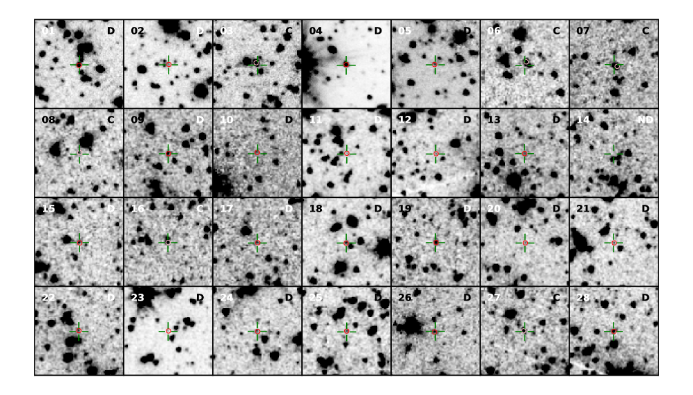
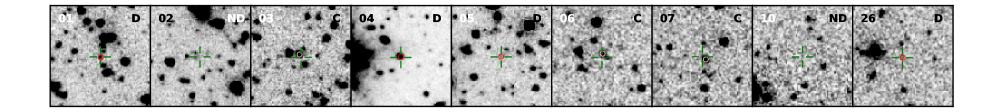
Figure 1: Spitzer/IRAC 3.6 $\mu$m (4.5 $\mu$m) imaging for 28 (9) metal-poor galaxies illustrated on top (bottom) panel. Of the galaxies with 3.6 $\mu$m (4.5 $\mu$m) data, 21 (four) were detected (“D”), one (two) was not detected (“ND”), and six (three) suffer from confusion/blending with nearby sources (“C”). The targeted galaxies are at the centre of the images. Green crosshairs mark the optical position of the galaxies. These positions were improved by Matthews et al. (2013) using SDSS and CFHT data. Red circles (radius of 1$\aas@@fstack{\prime\prime}$5) mark the IRAC position, and pink circles (radius of 1$\aas@@fstack{\prime\prime}$5) mark the closest object found by MOPEX to the optical position for blended cases. Each image is 40″ on a side, which corresponds to an angular distance of 300 kpc at $z=0.8$, and oriented such that North is up and East is left.

Table 1: Summary of Spitzer/IRAC Observations and Photometry

ID	R.A.	Declination	Obs. Date	Int. Time	$F$([3.6])tn:1	$F$([4.5])tn:1	IRAC Det.	Aper. Corr.
	hh:mm:ss.ss	dd:mm:ss.ss		(min)	($\mu$Jy)	($\mu$Jy)
(1)	(2)	(3)	(4)	(5)	(6)	(7)	(8)	(9)
01	14:18:31.26	52:49:42.49	…tn:2	227/230tn:3	4.30$\pm$0.14	2.86$\pm$0.18	Yes/Yes	1.55/1.53
02	14:21:21.53	53:01:07.84	…tn:2	113/127tn:3	2.47$\pm$0.22	$<$0.64tn:4	Yes/No	1.55/1.50
03	14:21:25.48	53:09:48.09	…tn:2	143/136tn:3	…	…	Conf./Conf.	1.55/1.62
04	14:22:03.72	53:25:47.77	…tn:2	103/125tn:3	35.04$\pm$0.24	27.80$\pm$0.27	Yes/Yes	1.55/1.64
05	14:21:45.40	53:23:52.71	…tn:2	152/147tn:3	3.49$\pm$0.18	2.58$\pm$0.20	Yes/Yes	1.57/1.66
06	16:47:26.17	34:45:11.89	…tn:2	115/113tn:3	…	…	Conf./Conf.	1.64/1.65
07	16:46:35.40	34:50:27.82	…tn:2	113/113tn:3	…	…	Conf./Conf.	1.67/1.65
08	16:47:26.47	34:54:09.55	2016-05-26	125/…tn:5	…	…	Conf./…tn:5	1.62/…tn:5
09	16:49:51.35	34:45:18.05	2016-05-26	129/…tn:5	3.60$\pm$0.30	…	Yes/…tn:5	1.54/…tn:5
10	16:51:31.45	34:53:15.83	…tn:2	114/114tn:3	2.73$\pm$0.36	$<$1.87tn:4	Yes/No	1.63/1.70
11	16:50:55.32	34:53:29.66	2016-05-26	156/…tn:5	1.36$\pm$0.24	…	Yes/…tn:5	1.47/…tn:5
12	16:53:03.46	34:58:48.71	2016-05-26	156/…tn:5	1.30$\pm$0.40	…	Yes/…tn:5	1.51/…tn:5
13	16:51:24.04	35:01:38.54	2016-05-26	126/…tn:5	2.02$\pm$0.30	…	Yes/…tn:5	1.57/…tn:5
14	16:51:20.32	35:02:32.39	2016-05-26	126/…tn:5	$<$0.92tn:4	…	No/…tn:5	1.58/…tn:5
15	23:27:20.38	00:05:54.40	2016-03-07	156/…tn:5	1.77$\pm$0.30	…	Yes/…tn:5	1.67/…tn:5
16	23:27:43.14	00:12:42.45	2016-03-07	114/…tn:5	…	…	Conf./…tn:5	1.74/…tn:5
17	23:27:29.87	00:14:19.94	2016-03-07	114/…tn:5	2.03$\pm$0.40	…	Yes/…tn:5	1.67/…tn:5
18	23:27:07.50	00:17:41.16	2016-03-07	130/…tn:5	4.39$\pm$0.50	…	Yes/…tn:5	1.72/…tn:5
19	23:26:55.43	00:17:52.68	2016-09-14	156/…tn:5	3.63$\pm$0.36	…	Yes/…tn:5	1.77/…tn:5
20	23:30:57.95	00:03:37.92	2016-09-13	156/…tn:5	1.15$\pm$0.39	…	Yes/…tn:5	1.79/…tn:5
21	23:31:50.74	00:09:38.91	2016-09-14	156/…tn:5	1.01$\pm$0.37	…	Yes/…tn:5	1.62/…tn:5
22	02:27:48.86	00:24:39.57	2016-10-27	156/…tn:5	1.76$\pm$0.31	…	Yes/…tn:5	1.62/…tn:5
23	02:27:05.71	00:25:21.54	2016-10-27	145/…tn:5	1.81$\pm$0.27	…	Yes/…tn:5	1.75/…tn:5
24	02:27:30.46	00:31:06.04	2016-10-27	151/…tn:5	1.81$\pm$0.37	…	Yes/…tn:5	1.70/…tn:5
25	02:26:03.72	00:36:21.98	2016-10-27	156/…tn:5	1.77$\pm$0.29	…	Yes/…tn:5	1.63/…tn:5
26	02:26:21.49	00:48:06.64	…tn:2	117/116tn:3	5.11$\pm$0.28	4.33$\pm$0.57	Yes/Yes	1.49/1.67
27	02:29:33.68	00:26:07.91	2016-10-27	153/…tn:5	…	…	Conf./…tn:5	1.62/…tn:5
28	02:29:02.03	00:30:07.83	2016-10-27	153/…tn:5	3.15$\pm$0.30	…	Yes/…tn:5	1.62/…tn:5

• (1): DEEP2 [O iii] $\lambda$4363 galaxy ID. (2): Right ascension. (3): Declination. (4): Observation date for new Spitzer/IRAC data. (5): Total on-source integration for 3.6 $\micron$ and 4.5 $\micron$ data, respectively. (6): Spitzer/IRAC 3.6 $\micron$ flux. (7): Spitzer/IRAC 4.5 $\micron$ flux. (8): Flags indicating whether galaxy was detected with Spitzer or confused (“Conf.”) for 3.6 $\micron$ and 4.5 $\micron$, respectively. (9): Aperture corrections for 3.6 $\micron$ and 4.5 $\micron$, respectively.

• Fluxes and uncertainties include aperture corrections given in Column (9).

• These galaxies were observed multiple times over many years.

• Integration times listed are the average exposure time from the Spitzer Heritage Archive images.

• 3$\sigma$ limits adopted.

• IRAC 4.5 $\mu$m observations are not available.

2.2 $\mathcal{MACT}$ Survey

To increase the sample size and extend toward lower stellar masses ($M_{\star}\lesssim 3\times 10^{9}$ $M_{\odot}$; DEEP2 is a magnitude-limited survey, $R<24.1$), we include the [O iii] $\lambda$4363-based samples from the $\mathcal{MACT}$ survey in our mass–metallicity relation analysis. Here, we briefly summarize the $\mathcal{MACT}$ sample and refer readers to Ly et al. (2016a) for more details.

The survey targeted $\approx$1,900 emission-line galaxies of the Subaru Deep Field ($\approx$0.25 deg² surveyed area; Kashikawa et al., 2004) that had excess flux in the narrow-band and/or intermediate-band filters (Ly et al., 2007). Using Keck and MMT, deep rest-frame optical spectra were obtained. The $\mathcal{MACT}$ survey consists of two sub-samples, those with detections of the [O iii] $\lambda$4363 line at S/N $\geq$ 3 ($N=29$ at $z\geq 0.5$) and those with upper limits on [O iii] $\lambda$4363 ($N=50$; $z\geq 0.5$). For the latter, Ly et al. (2016a) required that [O iii] $\lambda$5007 was detected at S/N $\geq$ 100 and [O iii] $\lambda$4363 at S/N $<$ 3. We refer to these two sub-samples collectively as the $\mathcal{MACT}$ sample.

The stellar masses for the $\mathcal{MACT}$ galaxies were determined with the Fitting and Assessment of Stellar Templates (FAST; Kriek et al., 2009) code using the following photometric data: (1) FUV and NUV imaging from GALEX (Martin et al., 2005); (2) $U$-band imaging from Kitt Peak National Observatory (KPNO) Mayall telescope using MOSAIC (Sawyer et al., 2010); (3) $BVR_{C}i^{\prime}z^{\prime}z_{b}z_{r}$ imaging from the Subaru telescope with Suprime-Cam (Miyazaki et al., 2002); (4) $H$-band imaging from KPNO Mayall telescope using NEWFIRM (Probst et al., 2008); and (5) $J$- and $K$-band imaging from UKIRT using WFCAM (Casali et al., 2007). Further discussion of the photometric data for $\mathcal{MACT}$ is provided in Ly et al. (2011) and Ly et al. (2016a). Together, the DEEP2 and $\mathcal{MACT}$ galaxies are at $z=0.578$ to $z=0.955$ with a median (mean) redshift of 0.789 (0.763).

3 Derived Measurements

3.1 Infrared Photometry

Using the MOsaicker and Point source EXtractor (MOPEX, vers. 18.5.6; Makovoz & Marleau, 2005), designed specifically to analyse Spitzer data, we performed aperture photometry to obtain the stellar continuum emission from the DEEP2 [O iii] $\lambda$4363-detected galaxies. We executed MOPEX mostly with default parameters with the following differences: not executing the fit_radius module, using a background-subtracted image for the point source probability (psp), adopting one aperture with a radius of 1$\aas@@fstack{\prime\prime}$8, and the values listed in Table 2 for the signal-to-noise ratio (SNR) in the select_conditions constraint. We then applied aperture corrections to obtain total photometric fluxes and calculated the background rms flux to estimate the uncertainty in the Spitzer images.

Table 2: Adopted SNR Threshold Values for Aperture Photometry with MOPEX

SNR	ID
(1)	(2)
3.0	04, 05, 08, 09, 10, 11, 12, 15, 16, 19, 21, 22, 23, 24, 25, 26, 27, 28
2.8	02, 03, 06, 07, 14, 18
2.5	13, 17, 20
2.0	01

• (1): Signal-to-noise ratio threshold used to identify sources by MOPEX (set in the select_conditions constraint). (2): DEEP2 [O iii] $\lambda$4363 galaxy ID. An SNR of 2.5 was used for all Spitzer 4.5$\mu$m images.

3.1.1 Total Spitzer Fluxes

The aperture corrections for the Spitzer/IRAC 3.6 $\mu$m and 4.5 $\mu$m photometry were determined as follows:
First, we identified bright stars in each image (within a radius of 6′ from the [O iii] $\lambda$4363-detected galaxy) using the coordinates of stars from the SDSS and cross-matched them against the Spitzer MOPEX catalogues. Stars were then rejected if they were (1) within 12″ of the edge of the image, (2) within 7″ of another object identified by MOPEX, or (3) if the MOPEX flux was below 400 $\mu$Jy in a circular aperture (1$\aas@@fstack{\prime\prime}$8, radius). These restrictions were used to limit our calculations to bright isolated stars. Fluxes were then calculated using a circular aperture ranging from a radius of 1 pixel (0$\aas@@fstack{\prime\prime}$6) to 9 pixels (5$\aas@@fstack{\prime\prime}$4). The latter was chosen to include as much starlight as possible while excluding the light of other sources. The aperture corrections were then derived from the ratio of the 9- to 3-pixel fluxes. Outliers contaminated by nearby sources were removed iteratively using a sigma-clipping approach ($\sigma=2.5$). The aperture correction, given in Table 1, is the mean from sigma clipping and has been applied to the IRAC fluxes in Table 1. If there were four or fewer stars within the search area after the restrictions, the aperture correction was set to the average correction (1.62 for both bands) of the remaining images. The 3.6 (4.5) $\mu$m aperture corrections range from 1.47 to 1.79 (1.50 to 1.68).

3.1.2 Measurements Uncertainties

To determine the uncertainty in the IRAC 3.6 $\mu$m and 4.5 $\mu$m detections, we computed the background rms flux in the Spitzer images. This was done by measuring the flux within randomly placed apertures throughout an image that has been masked for sources and then fitting the distribution of fluxes to obtain the Gaussian width. The Python package photutils.detect was used to construct a segmentation map to identify and mask pixels containing source emission. Here we required four contiguous pixels above a threshold value of 1.5$\sigma$. We then used photutils.aperture_photometry to measure the flux within a photutils.CircularAperture of three pixels (1$\aas@@fstack{\prime\prime}$8, radius) for 12000 random positions across the masked image (typically $\sim$7000 positions were not affected by emission from sources). The distribution of background fluxes was then constructed and mirroring of the lower half relative to the median or peak (whichever was lower) was performed. For 3.6 $\mu$m data, the 3$\sigma$ flux limits range between 0.42 and 1.49 $\mu$Jy, with a median and mean of 0.91 and 0.93 $\mu$Jy, respectively. For 4.5 $\mu$m data, 3$\sigma$ flux limits range between 0.51 and 1.87 $\mu$Jy with a median (mean) of 0.72 (1.01) $\mu$Jy. These limits are provided in Table 1.

Additionally, we visually inspected the Spitzer images to determine if the galaxy was detected and not blended with neighbouring sources. If the galaxy was not detected, we use the 3$\sigma$ background flux limit around the galaxy. If the galaxy was contaminated, we do not report a flux. Of the 28 galaxies, 21 were detected at 3.6 $\mu$m, one was not detected, and six suffered contamination from nearby sources. Among the nine galaxies with 4.5 $\mu$m data, four were detected, two were not detected, and three were confused with nearby sources.

3.2 Stellar Masses

To estimate the stellar masses of DEEP2 [O iii] $\lambda$4363-detected galaxies, we combine Spitzer measurements with optical and near-infrared data, to model the SED of each galaxy. We describe below the photometric data (Section 3.2.1), the adopted SED models (Section 3.2.2), assumptions in our SED fitting (Section 3.2.3), and stellar mass comparisons (Section 3.2.4).

3.2.1 Optical and Near-Infrared Data

The optical and near-infrared data, provided in Table 3, include Canada-France-Hawaii Telescope (CFHT) $BRI$ photometry from Coil et al. (2004), $ugriz$ from Matthews et al. (2013), $JHK_{s}$ for DEEP2 #01 from the NEWFIRM Medium-Band Survey (Whitaker et al., 2011), and $K_{s}$ photometry for DEEP2 #04 from Bundy et al. (2006).

These photometric data have been corrected for nebular emission lines from optical spectroscopy using the technique described in Ly et al. (2015b) and Ly et al. (2016a). For our sample, this correction can be significant due to the strong H$\beta$+[O iii] emission such that it can over correct redder optical band(s), such as $z$-band. To avoid this overcorrection, we perform the SED modelling excluding the affected band(s).

3.2.2 SED Modelling

Models. The stellar synthesis models were created in Python using Code Investigating GALaxy Emission, (CIGALE, vers. 0.9.0; Noll et al., 2009), an open-source software that has been well tested. The models assumed a Bruzual & Charlot (2003, hereafter BC03) simple stellar population (SSP), Chabrier (2003) initial mass function (IMF), and a “delayed $\tau$” star formation history:

$${\rm SFR}(t)\propto\frac{t}{\rm\tau_{main}^{2}}\exp{\left(\frac{-t}{\rm\tau_{main}}\right)},$$ (1)

where ${\rm\tau_{main}}$ is the $e$-folding time of the main stellar population. Here, the SFR rises steadily, peaks at $t={\rm\tau_{main}}$, and then declines exponentially.

In addition, we assumed a stellar metallicity of 0.02, a power-law dust attenuation with a slope of –0.7 (Charlot & Fall, 2000), and an old-to-young stellar population reduction factor in $A_{V}$ of 0.44. We did not include an active galactic nuclei (AGN) model or the 2175 Å bump in the fitting, and the nebular component is excluded (see Section 3.2.1). The models also included a separation age between young and old stars of 10 Myr (default value for CIGALE). We defer discussions on our choices in SSP models and star formation histories to Section 3.2.3.

Physical Parameters. The modelled parameters are listed in Table 4. Here we provide a brief discussion of the physical stellar population parameters and refer readers to Noll et al. (2009) for more information. The $t_{\rm age}$ parameter is the age of the oldest stars in the galaxy. The values for ${\rm\tau_{main}}$ and $t_{\rm age}$ were chosen to allow for a wide range (star-forming to passive) of possible star formation histories. The $A_{V}$ parameter measures the V-band attenuation for the young stellar population used in the dust attenuation model. The values for $A_{V}$ were chosen to allow for a broad range of possible attenuation corrections, from zero reddening to three magnitudes.

Using these adopted parameters, CIGALE created thousands of models for each galaxy and determined the best fitting model using a Bayesian-like approach. A Bayesian methodology provides robust estimates on the physical properties, their associated uncertainties, and accounts for degeneracies between parameters by weighting each model by their $\chi^{2}$ (Boquien et al., 2019). The results of the SED modelling are summarized in Table 5. We illustrate in Figure 2 the SED-fitting result from CIGALE for one of our galaxies, DEEP2 #18.

We note that the SED results for DEEP2 #04 and #14 are not used. The SED models for these galaxies are not well constrained due to their limited photometric dataset. DEEP2 #04 is a very bright galaxy that its optical measurements are not available in the DEEP2 catalogs. DEEP2 #14 was not detected by Spitzer/IRAC, thus limiting its photometric dataset to three bands (BRI) and an upper limit at 3.6 $\mu$m. The upper limit is far below the BRI photometry, causing a poor fit ($\chi^{2}_{\nu}=5.7$).

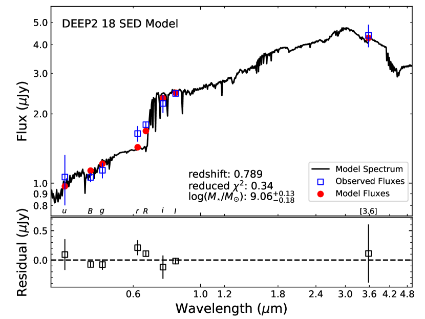
Figure 2: Top: The best-fit spectral synthesis model constructed by CIGALE for DEEP2 #18. The rightmost blue square is the new Spitzer/IRAC 3.6 $\micron$ photometry. Bottom: Difference between observed and model fluxes.

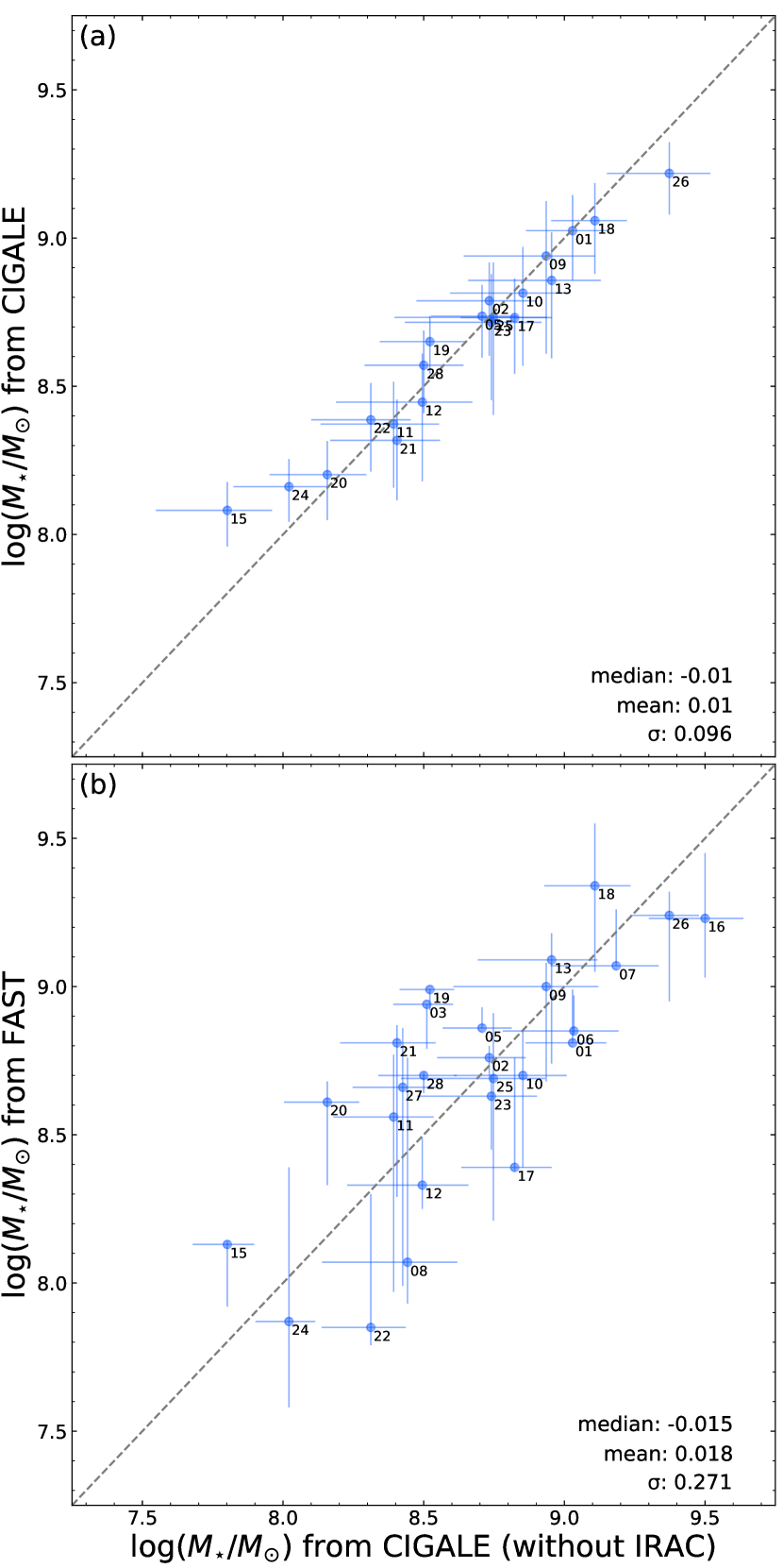
Figure 3: (a) Comparison between stellar masses derived from CIGALE with and without IRAC photometry. Blue circles are $z\approx 0.8$ DEEP2 galaxies with IRAC detections (3.6 $\mu$m or 3.6 and 4.5 $\mu$m). Galaxies with confused measurements are excluded. Good agreement is seen between stellar masses derived with and without infrared photometry. (b) Comparison between stellar masses derived from CIGALE and FAST (see Ly et al. 2015b) without the use of Spitzer/IRAC photometry. The grey dashed line marks one-to-one. The median, mean, and $\sigma$ values are calculated from the difference in mass between the two stellar mass estimates illustrated here. Generally, these mass estimates using different SED fitting code agree within measurement uncertainties.

3.2.3 Explanations for Assumptions in SED Fitting

There are two reasons why we chose the BC03 SSP model. First, it is more commonly used for galaxy evolution studies, which enable direct comparisons to earlier studies. Specifically, we will later compare our work against the local $M_{\star}$–$Z$ relation of AM13, which used stellar masses determined with the BC03 SSP model (Kauffmann et al., 2003).

Second, BC03 is the more conservative choice, as CIGALE only supports the BC03 and Maraston (2005, hereafter M05) SSP models. M05 was one of the first SSP models to include the thermally-pulsating asymptotic giant branch (TP-AGB) phase. TP-AGB stars heavily affect the SED of galaxies at stellar ages of about 1 to 3 Gyr. Its effects are still debated (e.g., Kriek et al., 2010; Capozzi et al., 2016, and references therein); we refer readers to Conroy et al. (2009), which discussed differences in physical properties for these models.

We note that this age range is generally older than the ages of our galaxies, given our emission-line selection, thus TP-AGB stars are not expected to have a significant effect in our modelling. This is supported by the fact that stellar masses, which we derived with the M05 SSP, are only systematically lower by a median (mean) value of 0.14 (0.13) dex compared to BC03 (assuming a Salpeter (1955) IMF for both models).

A delayed $\tau$ star formation history is well-suited for young galaxies with ages < $\tau$ and is commonly used for both star-forming and quiescent galaxies at high redshifts (e.g., Papovich et al., 2011; Pacifici et al., 2013; Lee et al., 2015, 2018; Estrada-Carpenter et al., 2019). Furthermore, with our limited photometric dataset, other star formation histories, such as those with episodic bursts, have more degrees of freedom to constrain.

3.2.4 Stellar Mass Comparisons

In panel (a) of Figure 3, we examine how the new Spitzer/IRAC observations constrain the masses of the 28 galaxies. Here, we illustrate the masses derived from CIGALE including and excluding the new Spitzer/IRAC observations. As illustrated, the stellar masses estimated with or without the new observations are consistent for most of the galaxies with a dispersion below 0.1 dex. This suggests that the other galaxies without Spitzer measurements have robust stellar mass estimates from mostly optical data. In panel (b) of Figure 3, we compare stellar masses calculated from CIGALE and a different SED fitting code, FAST (Kriek et al., 2009). These FAST estimates were derived by Ly et al. (2015b). To compare directly, we do not include the new Spitzer/IRAC 3.6 and 4.5 $\micron$ observations. While there are differences between the FAST and CIGALE estimates, there is generally good agreement with a dispersion of 0.27 dex. The good agreement between CIGALE and FAST indicates that we are able to conduct our $M_{\star}$–$Z$ analysis with the DEEP2 and $\mathcal{MACT}$ samples.

In addition, we compare our stellar mass estimates against those obtained from modelling DEEP2 optical spectra (Comparat et al., 2017, hereafter C17). Here we briefly summarize the sample and modelling, and refer readers to C17 for more details. From the fourth DEEP2 data release, $\approx$23,000 unique galaxy spectra were selected with a redshift between 0.7 and 1.2. SED models were created using the FIREFLY fitting code (Wilkinson et al., 2017), which uses a Maraston & Strömbäck (2011) SSP, three different stellar libraries, and three different IMFs. In the below comparisons, we adopt a Salpeter (1955) IMF for all stellar mass estimates, and use the C17 estimates that adopted the STELIB stellar library (Le Borgne et al., 2003).

Out of our 28 DEEP2 galaxies, 27 were modelled by C17 (DEEP2 #15 was not modelled). For BC03, we find that C17 stellar masses were higher by a median (mean) value of 0.47 (0.44) dex. For M05, C17 stellar masses were again higher by a median (mean) value of 0.62 (0.56) dex. The higher stellar masses measured by C17 is possibly due to the inability to constrain the Balmer stellar absorption lines. Specifically C17 masked regions affected by nebular emission lines, which included the Balmer lines. The best fits revealed significant stellar absorption, which was not seen from double Gaussian fitting by Ly et al. (2015b). We note that the average stellar mass uncertainty from C17 is 0.62 dex. This uncertainty is larger than that obtained from modelling broadband optical and infrared data (0.17 dex). One of the factors contributing to the larger uncertainty is that obtaining significant detection of the continuum with spectroscopy is more difficult for these low-mass galaxies.

3.3 $T_{e}$-based Oxygen Abundances

Both [O iii] $\lambda$4363 and [O iii] $\lambda$5007 are collisionally excited emission lines where their flux ratio is dependent on the free electron kinetic temperature of the ionized gas, $T_{e}$. The cooling of the gas is controlled by collisional excitation of ionized atoms, such as single and doubly ionized oxygen, and radiation from these excited states. However, for metal-poor gas, cooling is difficult with the lack of ionized metals. Thus, the electron temperature of the gas is high and results in more collisions to the excited doubly-ionized oxygen state that produces the [O iii] $\lambda$4363 emission (Aller, 1984). The gas-phase metallicity for our galaxies was determined by Ly et al. (2015b) by following previous direct metallicity studies and using the empirical relations of Izotov et al. (2006). Here, we briefly summarize the approach, and we refer readers to Ly et al. (2014) for more details. The electron temperature is determined from the flux ratio of [O iii] $\lambda$$\lambda$4959,5007 against [O iii] $\lambda$4363. Using $T_{e}$ and two emission-line flux ratios, [O ii] $\lambda$$\lambda$3726,3729/H$\beta$ and [O iii] $\lambda$$\lambda$4959,5007/H$\beta$, the oxygen-to-hydrogen ratio (O/H) can be determined. A standard two-zone temperature model with $T_{e}$(O⁺) = 0.7$T_{e}$(O⁺⁺) + 3000 K was adopted (AM13). The median, mean, and dispersion in metallicity for the DEEP2 galaxies are $12+\log({\rm O/H})=8.17$, 8.1, and 0.26, respectively.

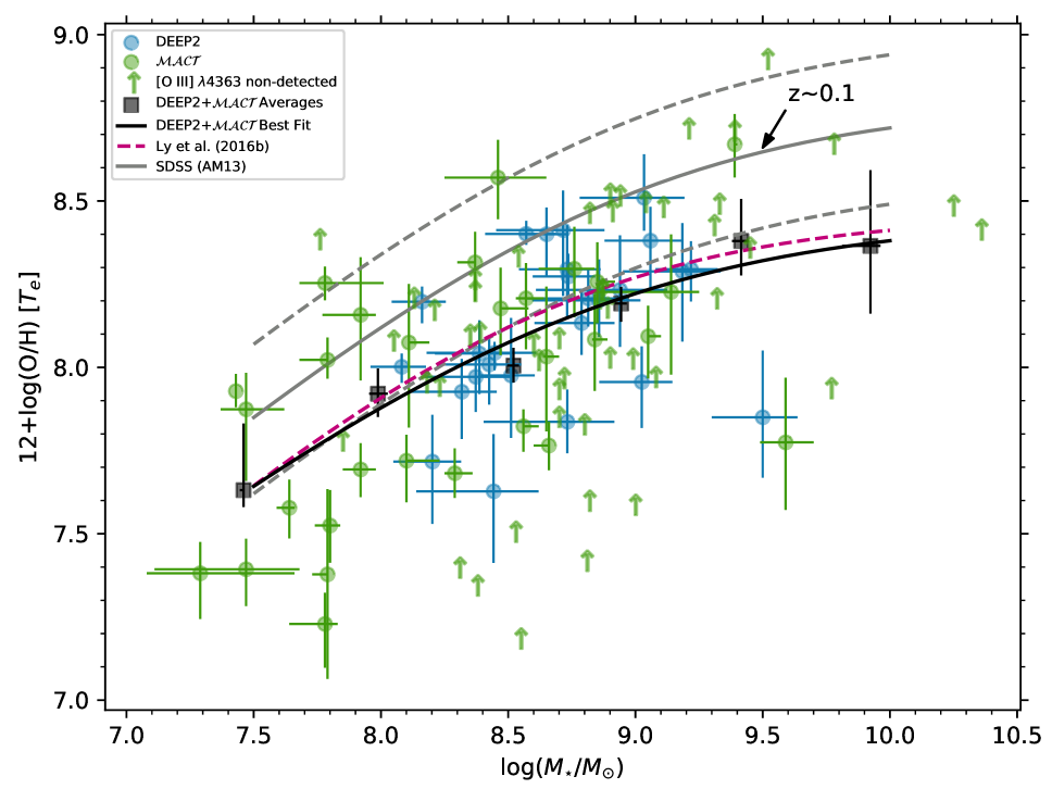
Figure 4: Oxygen abundance as a function of stellar mass. Blue circles are $z\approx 0.8$ DEEP2 galaxies from this study. Green circles and green arrows are the $\mathcal{MACT}$ [O iii] $\lambda$4363-detected and non-detected samples, respectively. The DEEP2 and $\mathcal{MACT}$ galaxies are binned in stellar mass (see Table 6), and the resulting average mass and metallicity of the bins are shown as black squares with their corresponding uncertainty. The binned points are fitted to Equation (2) (black line; see Figure 5 for fitting results). We compare our $M_{\star}$–$Z$ relation to SDSS galaxies from AM13 (solid grey line, with grey dashed lines enclosing $\pm$1$\sigma$), and the DEEP2+$\mathcal{MACT}$ relation from Ly et al. (2016b) (dashed magenta line).

4 Results

We describe below the stellar population of these low-metallicity galaxies (Section 4.1), measurements of the $M_{\star}$–$Z$ relation (Section 4.2), comparisons to previous studies (Section 4.3), dependence on SFR for the $M_{\star}$–$Z$ relation (Section 4.4), and the selection function of our study (Section 4.5).

4.1 Stellar Population

The 28 galaxies in our sample were originally classified as low-mass galaxies based on their optical photometry. However, infrared data is needed to observe the low-mass stars in these galaxies. Using the 3.6 $\micron$ (and 4.5 $\micron$ where available) photometry from Spitzer/IRAC and existing optical data, our SED models have confirmed that the 28 galaxies have low masses, with stellar masses between $\log(M_{\star}/M_{\odot})$=8.08 and 9.50 with a median (mean) of 8.72 (8.69). The good agreement in stellar mass measurements with and without Spitzer infrared data, as illustrated in Figure 3(b), suggests that there is no evidence for an old ($\gtrsim$1 Gyr) population of low-mass stars in these galaxies. This result is driven primarily by the low luminosities observed at rest-frame 2 $\mu$m.

We note that we considered bottom-heavier IMFs by running CIGALE with a Salpeter (1955) IMF. As expected, the masses with the Salpeter (1955) IMF are systematically higher by 0.22 dex. While the stellar masses are higher, the results still support the lack of a significant old population of low-mass stars in these galaxies.

For our sample, we have spectroscopic measurements of H$\beta$ and higher-order Balmer lines (e.g., H$\gamma$, H$\delta$). These measurements allow us to measure the SFRs using the H$\beta$ luminosity corrected for dust attenuation using the H$\gamma$/H$\beta$ Balmer decrement (Ly et al., 2015b). Combining the Balmer-derived SFRs with derived stellar masses, the specific SFR (sSFR $\equiv$ SFR/$M_{\star}$) for these galaxies range from $\log{\left({\rm sSFR}/{\rm yr}^{-1}\right)}$ = –8.79 to –6.62 with a median and mean of –8.1 and –8.0, respectively.

4.2 $M_{\star}$–$Z$ Relation

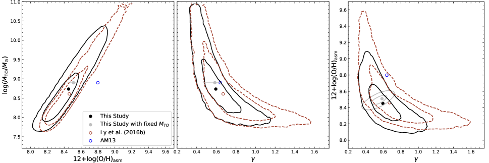
Figure 5: Confidence contours (68% and 95%) for the best fit parameters of the $M_{\star}$–$Z$ relation (see Table 7). Our fitting results for the $M_{\star}$–$Z$ relation are shown by solid black circles, while filled grey circles and grey contours are for $\log(M_{\rm TO}/M_{\odot})$ fixed to 8.901 from AM13. Overlaid in brown dashed lines and unfilled brown circles are the fitting results from Ly et al. (2016b). Blue unfilled circles are the best fit parameters from AM13.

In Figure 4, we examine the gas-phase metallicity dependence on stellar mass at $z\approx 0.8$ for the 28 DEEP2 galaxies and the $\mathcal{MACT}$ sample, and compare it against the $z\sim 0.1$ $M_{\star}$–$Z$ relation from AM13. Here we use the following formalism from Moustakas et al. (2011) to describe the shape of the $M_{\star}$–$Z$ relation:

$$12+\log({\rm O/H})=12+\log({\rm O/H})_{\rm asm}-\log\left[1+\left(\frac{M_{\rm TO}}{M_{\star}}\right)^{\gamma}\right],$$ (2)

where $\log({\rm O/H})_{\rm asm}$ is the asymptotic metallicity at the high-mass end, $M_{\rm TO}$ is the turnover mass in the $M_{\star}$–$Z$ relation, and $\gamma$ is the power-law slope at the low-mass end. We fit this equation to the average mass and metallicity of the DEEP2 galaxies and the $\mathcal{MACT}$ sample in each stellar mass bin. These averages are given in Table 6 and are illustrated in Figure 4 as black squares. In our fitting, we use a Monte Carlo approach where we repeat the fit 50 000 times using uncertainties obtained from the bootstrap method. In our fitting of the $M_{\star}$–$Z$ relation, we allow $M_{\rm TO}$ (1) to be a free parameter, and (2) fixed it to the local value from AM13. The results are given in Table 7, and confidence contours are illustrated in Figure 5.

Our best fit of the $M_{\star}$–$Z$ relation illustrates that there is a strong evolution between $z\sim 0.1$ and $z\approx 0.8$. At a given stellar mass, the $z\approx 0.8$ $M_{\star}$–$Z$ relation is lower than the relation from AM13 on average by 0.27 dex. This evolution follows $(1+z)^{-1.45^{+0.61}_{-0.76}}$. The overall shape of the $M_{\star}$–$Z$ relation between AM13 and our results is similar, comprising of a steep rise in metallicity at low stellar masses then transitioning to a plateau at high stellar masses. Additionally, the overall shape of the $M_{\star}$–$Z$ relation is consistent with the relation found by Ly et al. (2016b).

4.3 Comparison with Previous $z\approx 0.8$ $M_{\star}$–$Z$ Studies

Recent studies, such as Zahid et al. (2013, hereafter Z13) and Guo et al. (2016), have measured the evolution of the $M_{\star}$–$Z$ relation at intermediate redshifts. In these studies, strong-line metallicity diagnostics were used to determine chemical abundances. Specifically, Z13 used the Kobulnicky & Kewley (2004, hereafter KK04) calibration. Utilizing this calibration on our DEEP2 sample would yield metallicities that are 0.5–1 dex higher than those determined with the $T_{e}$ method. This suggests that the local KK04 calibration is not valid for metal-poor galaxies at $z\approx 0.8$. The use of different metallicity diagnostics inhibits a direct comparison against our results. However, relative comparisons against $z\approx 0.1$ measurements using the same metallicity diagnostics can be examined.

In Z13, a sample of 1254 galaxies at $0.75<z<0.82$ was selected from the third data release of the DEEP2 Galaxy Redshift Survey. Here, we briefly summarize the sample and refer readers to Z13 for more details. Among the $\sim$50,000 spectra, galaxies were selected with [O ii] $\lambda$3727 and H$\beta$ detections at S/N $>$ 3. In addition, 17 X-ray galaxies were removed to limit AGN contamination. Stellar masses were determined from BRI-band photometry, and average Balmer stellar absorption was corrected for each of the selected galaxies.

In Figure 6, we illustrate the evolution in metallicity as a function of stellar mass between $z\approx 0.1$ and $z\approx 0.8$ for Z13. Additionally, we extrapolate Z13 results to lower stellar masses using a linear fit, $\Delta Z$ $\propto$ 0.13 $\log(M_{\star}/M_{\odot})$, and compare it to the average evolution in metallicity of our samples (DEEP2, $\mathcal{MACT}$, and DEEP2+$\mathcal{MACT}$). Here we take the average metallicity of our samples due to a limited sample size and the effects of the selection function at high masses (see Section 4.5). As shown in the figure, our evolution in metallicity is in good agreement with the extrapolated evolution of Z13 toward lower stellar masses. The difference in $\Delta Z$ between Z13 and our study is expected, because we are sampling two different stellar populations. For reference, Z13 galaxies are higher mass galaxies with stellar masses between $\log(M_{\star}/M_{\odot})$ = 9.25 and 10.5, while our low-mass galaxies range from $\log(M_{\star}/M_{\odot})$ = 8.08 to 9.50. As illustrated in Figure 6, high-mass galaxies have accumulated most of their metallicity before $z\approx 0.8$. Between $z\approx 0.8$ and $z\approx 0.1$, the chemical evolution for Z13 is low, ranging from $\Delta Z$ = –0.21 to –0.08 dex. On the contrary, low-mass galaxies appear to undergo significant metal enrichment, with our samples (DEEP2, $\mathcal{MACT}$, and DEEP2+$\mathcal{MACT}$) at $\Delta Z$ = –0.29, –0.30, and –0.29 dex, respectively. Thus, a dwarf galaxy of $M_{\star}\approx 4\times 10^{8}$ $M_{\odot}$ at $z\approx 0.8$ undergoes 1.6 times more enrichment than a massive galaxy of $M_{\star}\approx 10^{10}$ $M_{\odot}$ at the same redshift.

As a further test, we can directly compare our evolution in the $M_{\star}$–$Z$ relation to Ly et al. (2016b). We determined that the $M_{\star}$–$Z$ relation follows a $(1+z)^{-1.45^{+0.61}_{-0.76}}$ evolution, such that metallicity is lower by $\approx$0.27 dex at $z\approx 0.8$ compared to $z=0.1$. This evolution is in agreement, within measurement uncertainties, of Ly et al. (2016b): $(1+z)^{-2.32^{+0.52}_{-0.26}}$. We note that the higher dependence measured by Ly et al. (2016b) is due to a higher (i.e., more enriched) $M_{\star}$–$Z$ relation at $z\approx 0.07$ than AM13.

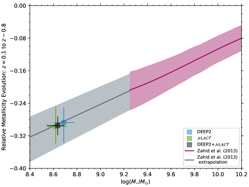
Figure 6: Relative metallicity evolution ($\Delta\log({\rm O/H})$) in the $M_{\star}$–$Z$ relation as a function of stellar mass. The blue, green, and black squares are the average $T_{e}$-based metallicity for DEEP2 galaxies from this study, $\mathcal{MACT}$ galaxies, and DEEP2 and $\mathcal{MACT}$, respectively. We compare our results to Z13 (magenta line with shaded region enclosing $\pm$1$\sigma$), which used strong-line metallicity diagnostics. In both studies, relative evolution is derived from SDSS ($z\approx 0.1$). Additionally, we extrapolate Z13 results to lower stellar masses (grey line with shaded region enclosing $\pm$1$\sigma$). The evolution in our $M_{\star}$–$Z$ relation is in good agreement with the extrapolation of Z13 results toward lower stellar masses. This demonstrates that lower mass galaxies build up their interstellar metal content more recently.

4.4 SFR Dependence

The idea that the $M_{\star}$–$Z$ relation has a secondary dependency on the SFR has been proposed by a number of observational and theoretical studies (e.g., Ellison et al., 2008; Lara-López et al., 2010; Mannucci et al., 2010; Davé et al., 2011; Lilly et al., 2013; Salim et al., 2014). Specifically, it has been suggested that higher SFRs can account for the lower metal abundances at higher redshifts, such that the $M_{\star}$–$Z$ relation is part of a larger non-evolving metallicity relation. To test this idea, we follow the approach of adopting a non-parametric method of projecting the $M_{\star}$–$Z$–SFR relation onto two-dimensional spaces. This was first implemented by Salim et al. (2014) and later applied to higher redshifts by Salim et al. (2015) and Ly et al. (2016b).

First, we consider how the $M_{\star}$–$Z$ relation depends on sSFR, which we illustrate in the left panel of Figure 7. The $M_{\star}$–$Z$ relation is divided into two sSFR bins, at the median of our DEEP2+$\mathcal{MACT}$ galaxies. Average measurements from composite spectra of AM13 are overlaid as grey squares. For reference, the local $M_{\star}$–$Z$ relation of AM13 is shown by the grey line. At a given stellar mass, the left panel of Figure 7 suggests that the metallicity for $z\approx 0.8$ low-mass galaxies does not decrease as the (s)SFR increases.

Next, we consider how the metallicity and sSFR depend on mass. This is illustrated in the right panel of Figure 7. The galaxies are divided into two stellar mass bins, at the median of our samples. Galaxies from AM13 are overlaid as grey squares. In each stellar mass bin, the galaxies from AM13 demonstrate that there is a moderate negative correlation between metallicity and sSFR, as expected. However, the metallicities of the DEEP2+$\mathcal{MACT}$ galaxies do not decrease as the sSFRs increase. In the lower mass bin, there are a number of low-sSFR and low-metallicity galaxies ($12+\log({\rm O/H})\sim 7.5$), which go against what is predicted by Mannucci et al. (2010).

Finally, we consider how the $M_{\star}$–SFR relation depends on metallicity. This is illustrated in the left panel of Figure 8. The galaxies are divided into four $12+\log({\rm O/H})$ bins ranging from 7.19 to 9.09. Galaxies from AM13 are overlaid as grey squares. The right panel of Figure 8 illustrates the sSFR dependence on metallicity. The average values of sSFR, illustrated in the left panel, are overlaid as black squares in the right panel. We fit our DEEP2+$\mathcal{MACT}$ [O iii] $\lambda$43636-detected galaxies to a linear relation using scipy.optimize.curve_fit. This was repeated 40 000 times, perturbing the galaxies in metallicity and sSFR to account for measurement uncertainties. We find that the best fit is

$$\log({\rm sSFR})=-6.69^{+0.68}_{-0.76}-(0.17^{+0.09}_{-0.08})\cdot[12+\log({\rm O/H})].$$ (3)

For comparison, we run the same fitting analysis on the stacked results from AM13, and find a best fit of

$$\log({\rm sSFR})=10.24^{+0.17}_{-0.19}-(2.27\pm 0.02)\cdot[12+\log({\rm O/H})].$$ (4)

The shallower slope that we measure is due to (1) the selection function missing metal-rich low-sSFR galaxies (see Section 4.5), and (2) a population of extremely low metallicity galaxies that have relatively low sSFR. We note that the latter is not due to a selection bias since [O iii] $\lambda$4363 is more easily detected in low-metallicity, high-sSFR galaxies.

Our best fit yields $t=-2.04$ and $p=0.046$ for a linear regression t-test. Thus, it suggests that we cannot rule out the null hypothesis (i.e., no correlation) at $>$95% confidence. We note that a t-test of AM13 sSFR–$Z$ relation with our DEEP2+$\mathcal{MACT}$ data yields $t=25.5$ with $p<10^{-5}$ ($>$4$\sigma$). This suggests that we are able to rule out a strong sSFR–$Z$ dependence.

In summary, we conclude that the $M_{\star}$–$Z$ relation at $z\approx 0.8$ does not have a significant secondary dependence on SFR such that galaxies with higher sSFR have reduced metallicity. As illustrated in Figures 7 and 8, in each of the three projections, our galaxies display either a mild dependence or no dependence. Our result is in agreement with previous studies that have found a moderate or no SFR dependence of the $M_{\star}$–$Z$ relation (e.g., Pérez-Montero et al., 2013; de los Reyes et al., 2015; Salim et al., 2015; Guo et al., 2016; Sánchez et al., 2017). However, several studies have found a strong SFR dependence for galaxies in the local Universe (Lara-López et al., 2010; Lilly et al., 2013; Salim et al., 2014), and for high redshift galaxies, studies have found a similar trend but offset from the local relation (i.e. there is redshift dependence; Zahid et al., 2014; Salim et al., 2015).

4.5 [O iii] $\lambda$4363 Selection Function

The requirement to detect [O iii] $\lambda$4363 in our spectroscopic study leads to a concern of selection bias for our samples. Here, we briefly outline the effects on our results. We refer readers to Ly et al. (2016b) for an in-depth analysis.

The detection of the [O iii] $\lambda$4363 line is dependent on a combination of (1) the electron temperature/metallicity of the gas (Nicholls et al., 2014), and (2) the dust-corrected SFRs which determine the absolute strengths of the emission-line fluxes. At high SFRs, [O iii] $\lambda$4363 is detectable for a wide range of metallicities. As SFR decreases, only metal-poor galaxies can be detected in an emission-line flux-limited survey. The effects of the [O iii] $\lambda$4363 selection function is illustrated in the right panel of Figure 8 where sSFR decreases as metallicity increases, but at a lower rate than AM13. The difference in the slopes is the result of two factors at high and low metallicities. First, there is a selection toward metal-rich galaxies with high SFRs because those with low SFRs will not have [O iii] $\lambda$4363 detections and will fall below the flux limit cuts adopted by Ly et al. (2015b). Second, the DEEP2+$\mathcal{MACT}$ sample is lacking low-metallicity, high-sSFR galaxies. Unlike their metal-rich counterparts, these galaxies have detectable [O iii] $\lambda$4363 measurements.

5 Conclusions

We present new Spitzer/IRAC 3.6 $\micron$ (4.5 $\micron$ where available) photometry for 28 metal-poor strongly star-forming galaxies at $z\approx 0.8$ from the DEEP2 Survey. These new measurements were necessary to better constrain the stellar masses of these galaxies by observing the light from low-mass stars. Our SED modelling of 0.35–3.6(4.5) $\mu$m data confirmed that these galaxies have low stellar masses, $M_{\star}\approx 10^{8.1}$–10^9.5 $M_{\odot}$.

Combining these stellar masses with metal abundances derived from the electron temperature method, and measurements from the $\mathcal{MACT}$ Survey, we determined that the $M_{\star}$–$Z$ relation evolves toward lower metallicity by $\approx$0.27 dex between $z\approx 0.8$ and $z=0.1$: $\propto$$(1+z)^{-1.45^{+0.61}_{-0.76}}$. Our evolution is in agreement within measurement uncertainties of Ly et al. (2016b): $\propto(1+z)^{-2.32^{+0.52}_{-0.26}}$. We compared the evolution in metallicity from $z\approx 0.8$ to $z\approx 0.1$ against recent studies at intermediate redshifts. Specifically, we find good agreement with those reported by Z13 when extrapolated toward lower stellar masses. This suggests that lower mass galaxies ($4\times 10^{8}$ $M_{\odot}$) chemically enriched their interstellar contents 1.6 times more rapidly than high mass galaxies ($10^{10}$ $M_{\odot}$). Additionally, we measured the shape of the $M_{\star}$–$Z$ relation at $z\approx 0.8$, which is consistent with the shape of local relation (AM13). Finally, we considered whether the $M_{\star}$–$Z$ relation has a secondary dependence on specific SFR. We determined an sSFR–$Z$ relation of: $\log({\rm sSFR})=-6.69^{+0.68}_{-0.76}-(0.17^{+0.09}_{-0.08})\cdot[12+\log({\rm O/H})]$. A linear t-test determined that we cannot rule out no dependence at $>$95% confidence. However, a strong dependence, as determined for local galaxies (AM13), can be ruled out at $>$4$\sigma$ confidence.

Table 3: Optical and Near-Infrared Photometry for [O iii] $\lambda$4363-detected DEEP2 Galaxies

ID	$u$	$B$	$g$	$r$	$R$	$i$	$I$	$z$	$J$	$H$	$K_{s}$
(1)	(2)	(3)	(4)	(5)	(6)	(7)	(8)	(9)	(10)	(11)	(12)
01	1.58	1.88	1.94	2.04	2.16	3.02	2.96	3.27	4.26	3.37	3.21
	$\pm$0.02	$\pm$0.05	$\pm$0.10	$\pm$0.01	$\pm$0.04	$\pm$0.02	$\pm$0.07	$\pm$0.05	$\pm$0.20	$\pm$0.18	$\pm$0.18
02	0.83	0.93	0.94	1.10	1.01	1.79	1.62	1.48	…	…	…
	$\pm$0.02	$\pm$0.08	$\pm$0.01	$\pm$0.02	$\pm$0.05	$\pm$0.02	$\pm$0.12	$\pm$0.06	…	…	…
03	0.44	0.76	0.67	0.79	0.75	1.04	1.06	1.29	…	…	…
	$\pm$0.01	$\pm$0.04	$\pm$0.01	$\pm$0.01	$\pm$0.03	$\pm$0.02	$\pm$0.05	$\pm$0.05	…	…	…
04	…	…	…	…	…	…	…	…	…	…	23.11
	…	…	…	…	…	…	…	…	…	…	$\pm$0.15
05	1.47	1.55	1.73	1.87	1.80	2.23	1.27tn:3a	0.35tn:3a	…	…	…
	$\pm$0.06	$\pm$0.04	$\pm$0.04	$\pm$0.07	$\pm$0.08	$\pm$0.11	$\pm$0.18	$\pm$0.17	…	…	…
06	…	1.58	…	…	2.23	…	3.13	…	…	…	…
	…	$\pm$0.03	…	…	$\pm$0.06	…	$\pm$0.15	…	…	…	…
07	2.05	2.74	3.03	2.90	3.50	4.07	5.02	1.20tn:3a	…	…	…
	$\pm$0.81	$\pm$0.03	$\pm$0.33	$\pm$0.45	$\pm$0.05	$\pm$0.70	$\pm$0.12	$\pm$1.87	…	…	…
08	…	0.77	…	…	0.91	…	1.10	…	…	…	…
	…	$\pm$0.03	…	…	$\pm$0.05	…	$\pm$0.13	…	…	…	…
09	…	0.93	…	…	1.21	…	1.90	…	…	…	…
	…	$\pm$0.03	…	…	$\pm$0.04	…	$\pm$0.10	…	…	…	…
10	…	1.44	…	…	1.73	…	2.30	…	…	…	…
	…	$\pm$0.03	…	…	$\pm$0.04	…	$\pm$0.09	…	…	…	…
11	…	0.87	…	…	0.96	…	1.09	…	…	…	…
	…	$\pm$0.03	…	…	$\pm$0.04	…	$\pm$0.11	…	…	…	…
12	…	0.76	…	…	0.86	…	1.20	…	…	…	…
	…	$\pm$0.03	…	…	$\pm$0.03	…	$\pm$0.08	…	…	…	…
13	…	0.75	…	…	1.00	…	1.69	…	…	…	…
	…	$\pm$0.04	…	…	$\pm$0.04	…	$\pm$0.10	…	…	…	…
14	…	1.33	…	…	1.66	…	2.05	…	…	…	…
	…	$\pm$0.04	…	…	$\pm$0.05	…	$\pm$0.10	…	…	…	…
15	1.02	1.38	1.16	1.19	0.91	0.55tn:3a	0.86	…	…	…	…
	$\pm$0.29	$\pm$0.05	$\pm$0.1	$\pm$0.14	$\pm$0.07	$\pm$0.22	$\pm$0.07	…	…	…	…
16	0.67	1.08	1.07	1.63	2.08	3.17	3.38	1.94tn:3a	…	…	…
	$\pm$0.29	$\pm$0.05	$\pm$0.09	$\pm$0.14	$\pm$0.05	$\pm$0.22	$\pm$0.06	$\pm$1.06	…	…	…
17	0.8	1.6	1.42	1.19	2.01	1.98	2.40	2.36	…	…	…
	$\pm$0.27	$\pm$0.06	$\pm$0.09	$\pm$0.13	$\pm$0.07	$\pm$0.20	$\pm$0.06	$\pm$0.98	…	…	…
18	1.06	1.06	1.14	1.64	1.80	2.22	2.45	1.66tn:3a	…	…	…
	$\pm$0.26	$\pm$0.05	$\pm$0.09	$\pm$0.13	$\pm$0.05	$\pm$0.2	$\pm$0.06	$\pm$0.95	…	…	…
19	1.6	1.69	2.13	2.10	1.85	2.23	1.87	2.04	…	…	…
	$\pm$0.32	$\pm$0.04	$\pm$0.11	$\pm$0.16	$\pm$0.08	$\pm$0.25	$\pm$0.07	$\pm$1.17	…	…	…
20	0.91	0.94	0.73	0.92	0.98	0.63	0.96	1.75tn:3a	…	…	…
	$\pm$0.28	$\pm$0.05	$\pm$0.09	$\pm$0.13	$\pm$0.07	$\pm$0.21	$\pm$0.07	$\pm$1.0	…	…	…
21	1.08	0.7	0.74	0.69	0.90	1.13	0.94	0.22tn:3a	…	…	…
	$\pm$0.29	$\pm$0.05	$\pm$0.10	$\pm$0.14	$\pm$0.05	$\pm$0.23	$\pm$0.09	$\pm$1.22	…	…	…
22	1.06	0.94	0.79	0.80	0.89	1.37	1.00	1.87	…	…	…
	$\pm$0.25	$\pm$0.07	$\pm$0.08	$\pm$0.11	$\pm$0.04	$\pm$0.18	$\pm$0.06	$\pm$0.84	…	…	…
23	0.93	0.84	0.69	0.92	0.94	1.73	1.34	1.97	…	…	…
	$\pm$0.22	$\pm$0.07	$\pm$0.09	$\pm$0.12	$\pm$0.04	$\pm$0.21	$\pm$0.07	$\pm$0.69	…	…	…
24	1.41	1.55	1.52	1.01	1.29	1.39	1.18	0.60tn:3a	…	…	…
	$\pm$0.24	$\pm$0.07	$\pm$0.10	$\pm$0.13	$\pm$0.04	$\pm$0.23	$\pm$0.06	$\pm$0.76	…	…	…
25	0.81	0.8	0.59	0.57	0.90	0.99	1.28	0.56tn:3a	…	…	…
	$\pm$0.21	$\pm$0.14	$\pm$0.09	$\pm$0.12	$\pm$0.05	$\pm$0.21	$\pm$0.08	$\pm$0.68	…	…	…
26	…	3.08	…	…	4.44	…	5.90	…	…	…	…
	…	$\pm$0.1	…	…	$\pm$0.06	…	$\pm$0.08	…	…	…	…
27	0.77	0.94	0.90	1.06	1.14	1.42	1.24	1.62tn:3a	…	…	…
	$\pm$0.23	$\pm$0.03	$\pm$0.09	$\pm$0.13	$\pm$0.04	$\pm$0.23	$\pm$0.06	$\pm$0.73	…	…	…
28	2.63	2.58	2.48	2.56	2.26	2.75	1.98tn:3a	1.75tn:3a	…	…	…
	$\pm$0.24	$\pm$0.03	$\pm$0.09	$\pm$0.13	$\pm$0.04	$\pm$0.22	$\pm$0.07	$\pm$0.73	…	…	…

• (1): DEEP2 [O iii] $\lambda$4363 galaxy ID. (2)–(12): Photometric fluxes from shorter to longer wavelengths. These photometric data are obtained from several studies: $BRI$ (Coil et al., 2004), $ugriz$ (SDSS or CFHT; Matthews et al., 2013), $JHK_{s}$ (for #01; Whitaker et al., 2011), and $K_{s}$ (for #04; Bundy et al., 2006). All fluxes are given in $\mu$Jy and have been corrected for nebular emission lines from optical spectroscopy using the technique described in Ly et al. (2014, 2016a).

• Fluxes are heavily affected by nebular emission line correction and not used in SED modelling.

Table 4: Adopted Parameters for SED Fitting with CIGALE

Parameter	Values
(1)	(2)
$\rm{\tau_{main}}$ (Myr)	250,500,1000,2000,4000,6000,8000
$t_{\rm age}$ (Myr)	10,25,50,75,100,125,150,175,200,225,250,500,1000,2000,4000,8000
$A_{V}$(young)	0.0,0.5,1.0,1.5,2.0,2.5,3.0

• (1): $\tau_{\rm main}$ is the e-folding time of the main stellar population model, $t_{\rm age}$ refers to the age of the oldest stars in the galaxy, and $A_{V}$(young) is the $V$-band attenuation of the young population. All other parameters were the default values set by CIGALE. (2): Allowed values for the SED modeling grid.

Table 5: Summary of SED-derived Stellar Properties from CIGALE

ID	$\log(M_{\rm\star}/M_{\rm\odot})$	SFR	SFR(10Myr)	SFR(100Myr)	$A_{\rm FUV}$	$A_{\rm{V}}$	$\tau_{\rm main}$	Age	$\chi^{2}_{\nu}$
	(dex)	($M_{\rm\odot}$/yr)	($M_{\rm\odot}$/yr)	($M_{\rm\odot}$/yr)	(mag)	(mag)	(Gyr)	(Myr)
(1)	(2)	(3)	(4)	(5)	(6)	(7)	(8)	(9)	(10)
01	$9.02^{+0.12}_{-0.17}$	9.66$\pm$8.31	9.27$\pm$5.66	7.52$\pm$4.05	1.52$\pm$0.54	0.53$\pm$0.21	3.14$\pm$2.81	390$\pm$388	1.06
02	$8.79^{+0.13}_{-0.19}$	2.45$\pm$1.64	2.41$\pm$1.48	2.13$\pm$1.04	0.91$\pm$0.72	0.31$\pm$0.25	3.38$\pm$2.79	915$\pm$736	1.71
03	$8.51^{+0.09}_{-0.12}$	12.17$\pm$11.2	9.90$\pm$6.49	6.60$\pm$5.35	3.39$\pm$0.80	1.35$\pm$0.38	3.18$\pm$2.77	…tn:2a	1.75
04	…	…	…	…	…	…	…	…	…
05	$8.74^{+0.11}_{-0.14}$	11.24$\pm$7.49	10.43$\pm$5.78	6.97$\pm$3.31	1.94$\pm$0.44	0.72$\pm$0.20	3.20$\pm$2.77	156$\pm$155	0.1
06	$9.03^{+0.16}_{-0.25}$	25.19$\pm$32.21	21.09$\pm$20.43	14.54$\pm$15.60	2.78$\pm$1.24	1.08$\pm$0.54	3.25$\pm$2.78	…tn:2a	0.03
07	$9.18^{+0.15}_{-0.23}$	34.72$\pm$39.05	29.90$\pm$25.25	20.33$\pm$18.67	2.44$\pm$1.01	0.93$\pm$0.44	3.22$\pm$2.78	…tn:2a	0.25
08	$8.44^{+0.18}_{-0.30}$	7.53$\pm$9.24	6.06$\pm$5.38	4.31$\pm$4.46	1.90$\pm$1.02	0.72$\pm$0.43	3.20$\pm$2.78	…tn:2a	0.01
09	$8.94^{+0.19}_{-0.33}$	12.91$\pm$13.26	11.83$\pm$8.83	8.17$\pm$6.31	2.68$\pm$0.91	1.02$\pm$0.39	3.28$\pm$2.77	…tn:2a	0.28
10	$8.81^{+0.16}_{-0.25}$	7.44$\pm$10.12	6.82$\pm$5.81	5.11$\pm$4.90	1.29$\pm$0.73	0.46$\pm$0.29	3.23$\pm$2.79	…tn:2a	0.23
11	$8.37^{+0.14}_{-0.21}$	4.78$\pm$5.52	4.25$\pm$3.21	2.93$\pm$2.62	1.27$\pm$0.66	0.46$\pm$0.27	3.16$\pm$2.78	…tn:2a	0.13
12	$8.45^{+0.16}_{-0.27}$	4.00$\pm$7.50	3.36$\pm$3.87	2.57$\pm$3.66	1.29$\pm$0.84	0.47$\pm$0.34	3.24$\pm$2.79	…tn:2a	0.05
13	$8.86^{+0.16}_{-0.26}$	7.87$\pm$21.38	5.85$\pm$10.66	5.08$\pm$10.53	1.68$\pm$1.07	0.60$\pm$0.44	3.24$\pm$2.79	…tn:2a	0.15
14tn:2b	…	…	…	…	…	…	…	…	…
15	$8.08^{+0.10}_{-0.12}$	3.81$\pm$1.69	3.51$\pm$1.37	2.05$\pm$0.77	0.79$\pm$0.54	0.29$\pm$0.21	3.16$\pm$2.77	90$\pm$52	2.65
16	$9.50^{+0.14}_{-0.20}$	33.44$\pm$70.79	27.53$\pm$36.26	23.22$\pm$34.89	3.66$\pm$1.09	1.39$\pm$0.50	3.27$\pm$2.79	…tn:2a	0.13
17	$8.73^{+0.13}_{-0.19}$	19.18$\pm$35.97	11.28$\pm$17.46	10.63$\pm$17.61	1.41$\pm$1.39	0.53$\pm$0.59	3.05$\pm$2.76	369$\pm$348	1.69
18	$9.06^{+0.13}_{-0.18}$	26.50$\pm$52.20	19.62$\pm$25.67	15.99$\pm$25.48	2.94$\pm$0.96	1.11$\pm$0.43	3.17$\pm$2.78	…tn:2a	0.34
19	$8.65^{+0.09}_{-0.11}$	15.70$\pm$6.49	14.27$\pm$5.08	8.35$\pm$2.89	1.79$\pm$0.46	0.68$\pm$0.19	3.17$\pm$2.77	84$\pm$57	0.93
20	$8.20^{+0.11}_{-0.15}$	4.12$\pm$3.17	3.70$\pm$2.19	2.40$\pm$1.46	1.13$\pm$0.56	0.42$\pm$0.23	3.20$\pm$2.78	135$\pm$109	0.84
21	$8.32^{+0.14}_{-0.20}$	4.46$\pm$7.12	3.64$\pm$3.70	2.74$\pm$3.44	1.06$\pm$0.72	0.39$\pm$0.30	3.16$\pm$2.78	225$\pm$218	0.63
22	$8.39^{+0.12}_{-0.17}$	5.33$\pm$3.09	4.97$\pm$2.47	3.15$\pm$1.37	1.69$\pm$0.58	0.63$\pm$0.24	3.20$\pm$2.78	…tn:2a	0.75
23	$8.72^{+0.16}_{-0.26}$	3.83$\pm$6.02	3.52$\pm$3.50	2.84$\pm$2.96	1.34$\pm$0.85	0.47$\pm$0.33	3.35$\pm$2.78	…tn:2a	0.57
24	$8.16^{+0.09}_{-0.12}$	4.08$\pm$1.77	3.79$\pm$1.44	2.26$\pm$0.76	0.76$\pm$0.51	0.28$\pm$0.19	3.16$\pm$2.77	104$\pm$62	1.02
25	$8.73^{+0.19}_{-0.33}$	4.12$\pm$6.10	3.83$\pm$3.67	2.95$\pm$3.02	1.59$\pm$0.94	0.57$\pm$0.37	3.41$\pm$2.80	…tn:2a	0.55
26	$9.22^{+0.11}_{-0.14}$	158.32$\pm$156.20	81.72$\pm$76.19	81.05$\pm$76.76	2.74$\pm$2.08	1.10$\pm$0.88	3.06$\pm$2.76	…tn:2a	0.14
27	$8.43^{+0.13}_{-0.18}$	9.08$\pm$10.38	7.00$\pm$5.51	5.06$\pm$4.98	2.04$\pm$0.92	0.78$\pm$0.40	3.17$\pm$2.78	…tn:2a	0.11
28	$8.57^{+0.12}_{-0.16}$	8.37$\pm$4.55	7.79$\pm$3.50	4.93$\pm$2.03	0.96$\pm$0.44	0.35$\pm$0.17	3.22$\pm$2.78	137$\pm$108	0.32

• (1): DEEP2 [O iii] $\lambda$4363 galaxy ID. (2): Stellar mass. (3)–(5): SFRs measured instantaneously, averaged over the last 10 Myr, and averaged over the last 100 Myr, respectively. (6)–(7): Dust attenuation in the FUV- and V-bands, respectively. (8): e-folding time for star formation. (9): Age of galaxy. (10): Reduced $\chi^{2}$ for best fit. Uncertainties are reported at the 16th and 84th percentile.

• Ages are not well constrained.

• SED model not well constrained due to the limited photometric dataset (e.g., 3 bands, $BRI$, and 1 limit, [3.6]).

Table 6: Binned DEEP2+$\mathcal{MACT}$ $M_{\star}$–$Z$ Relation

Bin	$N$	$\left<\log(M_{\star}/M_{\odot})\right>$	$\left<12+\log({\rm O/H})\right>$
(1)	(2)	(3)	(4)
7.5$\pm$0.25	5	$7.46^{+0.002}_{-0.01}$	$7.63^{+0.20}_{-0.05}$
8.0$\pm$0.25	19	$7.99^{+0.04}_{-0.03}$	$7.92^{+0.08}_{-0.07}$
8.5$\pm$0.25	36	$8.52^{+0.02}_{-0.03}$	$8.01^{+0.05}_{-0.05}$
9.0$\pm$0.25	32	$8.94^{+0.02}_{-0.03}$	$8.19^{+0.05}_{-0.06}$
9.5$\pm$0.25	9	$9.42^{+0.03}_{-0.04}$	$8.38^{+0.13}_{-0.10}$
10.0$\pm$0.25	3	$9.92^{+0.04}_{-0.11}$	$8.37^{+0.23}_{-0.20}$

• (1): Stellar mass bin. (2): Number of galaxies. (3): Average $\log(M_{\star}/$$M_{\odot}$$)$. (4): Average 12 + $\log({\rm O/H})$. Uncertainties are reported at the 16th and 84th percentile, and are determined using the bootstrapping method (described in Section 4.2).

Table 7: Best Fit for the $z\sim 1$ $M_{\star}$–$Z$ Relation

$\log\left(M_{\rm TO}/M_{\odot}\right)$	12 + $\log({\rm O/H})_{\rm asm}$	$\gamma$
(1)	(2)	(3)
$8.74^{+0.43}_{-0.83}$	$8.45^{+0.15}_{-0.25}$	$0.59^{+0.15}_{-0.21}$
8.901tn:1b	$8.51^{+0.06}_{-0.05}$	$0.59^{+0.09}_{-0.09}$

• Fitting parameters of the $M_{\star}$–$Z$ relation: (1) turnover mass, (2) asymptotic metallicity at the high stellar mass end, and (3) slope at the low-mass end. Uncertainties are reported at the 16th and 84th percentile, and are determined from the probability functions marginalized over the other two fitting parameters.

• $M_{\rm TO}$ was held fixed to the value determined by AM13.

Appendix A Mass–Metallicity–SFR Plots

In this appendix, we provide different projections of the mass–metallicity–SFR relation. Figure 7 compares gas metallicity against stellar mass (left panel) and sSFR (right panel). Here, binning was performed along sSFR and stellar mass, respectively. In Figure 8, we illustrate SFR as a function of stellar mass in different metallicity bins (left panel), and how the sSFR depends on metallicity (right panel).

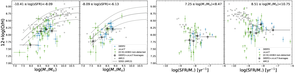
Figure 7: Oxygen abundance as a function of stellar mass (sSFR $\equiv$ SFR/$M_{\star}$) binned along sSFR (stellar mass) illustrated in the left (right) panel. Blue circles are $z\approx 0.8$ DEEP2 galaxies from this study. Green circles and green arrows are the $\mathcal{MACT}$ [O iii] $\lambda$4363-detected and non-detected samples, respectively. Black circles are the average metallicity and bootstrapped errors in bins with equal number (6–7) of [O iii] $\lambda$4363-detected galaxies. The range of the $x$ error bars is based on the minimum and maximum mass (sSFR) in each bin. Galaxies from AM13 are overlaid as grey squares. In the left panel, the $M_{\star}$–$Z$ relation from AM13 is shown by a solid grey line, with grey dashed lines enclosing $\pm$1$\sigma$. These projections illustrate that a strong dependence of the $M_{\star}$–$Z$ relation on sSFR, as seen in local galaxies, is not seen for these $z\approx 0.8$ galaxies.

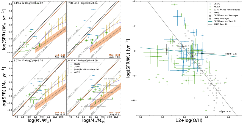
Figure 8: Left: SFR as a function of stellar mass for sub-samples binned according to oxygen abundance. Colour and point style schemes for galaxies follow those in Figure 7. The $M_{\star}$–$\rm{SFR}$ relation, determined by Salim et al. (2007) at $z\sim 0.1$, de los Reyes et al. (2015) at $z\approx 0.8$, and Whitaker et al. (2014) at $0.5<z<1$, are plotted as an orange band, yellow diamonds, and a purple line, respectively. Lines of constant inverse specific SFR (sSFR^-1) are shown as dashed grey lines with corresponding timescales. The median (average) sSFR^-1 of the DEEP2+$\mathcal{MACT}$ galaxies is shown as a brown (black) line, and the average is illustrated in the right panel. Right: Specific SFR as a function of metallicity. The black circles are the average sSFR in bins with equal number (13–14) of [O iii] $\lambda$4363-detected galaxies. Here the sSFR error bars are the bootstrapped averages while the metallicity error bars are based on the minimum and maximum in those bins. The turquoise (grey) line illustrates the least-squares fit for DEEP2+$\mathcal{MACT}$ (AM13). As shown, sSFR increases as metallicity decreases, but at a shallower slope than local galaxies. For DEEP2+$\mathcal{MACT}$, we performed t-tests that demonstrated that we cannot rule out zero sSFR–$Z$ dependence at $>$95%, but we are able to rule out the steep dependence found for local galaxies at $>$4$\sigma$ significance.

References

- Aller (1984) Aller, L. H. 1984, Astrophysics and Space Science Library, 112
- Amorín et al. (2015) Amorín, R., Pérez-Montero, E., Contini, T., et al. 2015, A&A, 578, A105
- Amorín et al. (2014) Amorín, R., Sommariva, V., Castellano, M., et al. 2014, A&A, 568, L8
- Andrews & Martini (2013) Andrews, B. H., & Martini, P. 2013, ApJ, 765, 140
- Astropy Collaboration et al. (2013) Astropy Collaboration, Robitaille, T. P., Tollerud, E. J., et al. 2013, A&A, 558, A33
- Atek et al. (2011) Atek, H., Siana, B., Scarlata, C., et al. 2011, ApJ, 743, 121
- Belli et al. (2013) Belli, S., Jones, T., Ellis, R. S., & Richard, J. 2013, ApJ, 772, 141
- Boquien et al. (2019) Boquien, M., Burgarella, D., Roehlly, Y., et al. 2019, A&A, 622, A103
- Bruzual & Charlot (2003) Bruzual, G., & Charlot, S. 2003, MNRAS, 344, 1000
- Bundy et al. (2006) Bundy, K., Ellis, R. S., Conselice, C. J., et al. 2006, ApJ, 651, 120
- Capozzi et al. (2016) Capozzi, D., Maraston, C., Daddi, E., et al. 2016, MNRAS, 456, 790
- Casali et al. (2007) Casali, M., Adamson, A., Alves de Oliveira, C., et al. 2007, A&A, 467, 777
- Chabrier (2003) Chabrier, G. 2003, PASP, 115, 763
- Charlot & Fall (2000) Charlot, S., & Fall, S. M. 2000, ApJ, 539, 718
- Coil et al. (2004) Coil, A. L., Newman, J. A., Kaiser, N., et al. 2004, ApJ, 617, 765
- Comparat et al. (2017) Comparat, J., Maraston, C., Goddard, D., et al. 2017, A&A, submitted (arXiv:1711.06575)
- Conroy et al. (2009) Conroy, C., Gunn, J. E., & White, M. 2009, ApJ, 699, 486
- Cullen et al. (2014) Cullen, F., Cirasuolo, M., McLure, R. J., Dunlop, J. S., & Bowler, R. A. A. 2014, MNRAS, 440, 2300
- Davé et al. (2011) Davé, R., Oppenheimer, B. D., & Finlator, K. 2011, MNRAS, 415, 11
- de los Reyes et al. (2015) de los Reyes, M. A., Ly, C., Lee, J. C., et al. 2015, AJ, 149, 79
- Ellison et al. (2008) Ellison, S. L., Patton, D. R., Simard, L., & McConnachie, A. W. 2008, ApJ, 672, L107
- Erb et al. (2006) Erb, D. K., Shapley, A. E., Pettini, M., et al. 2006, ApJ, 644, 813
- Estrada-Carpenter et al. (2019) Estrada-Carpenter, V., Papovich, C., Momcheva, I., et al. 2019, ApJ, 870, 133
- Fazio et al. (2004) Fazio, G. G., Hora, J. L., Allen, L. E., et al. 2004, ApJS, 154, 10
- Guaita et al. (2013) Guaita, L., Francke, H., Gawiser, E., et al. 2013, A&A, 551, A93
- Guo et al. (2016) Guo, Y., Koo, D. C., Lu, Y., et al. 2016, ApJ, 822, 103.
- Gwyn (2012) Gwyn, S. D. J. 2012, AJ, 143, 38
- Henry et al. (2013) Henry, A., Martin, C. L., Finlator, K., & Dressler, A. 2013, ApJ, 769, 148
- Hoyos et al. (2005) Hoyos, C., Koo, D. C., Phillips, A. C., Willmer, C. N. A., & Guhathakurta, P. 2005, ApJ, 635, L21
- Hu et al. (2009) Hu, E. M., Cowie, L. L., Kakazu, Y., & Barger, A. J. 2009, ApJ, 698, 2014
- Hunt et al. (2012) Hunt, L., Magrini, L., Galli, D., et al. 2012, MNRAS, 427, 906
- Izotov et al. (2006) Izotov, Y. I., Stasińska, G., Meynet, G., Guseva, N. G., & Thuan, T. X. 2006, A&A, 448, 955
- Jones et al. (2015) Jones, T., Martin, C., & Cooper, M. C. 2015, ApJ, 813, 126
- Kashikawa et al. (2004) Kashikawa, N., Shimasaku, K., Yasuda, N., et al. 2004, PASJ, 56, 1011
- Kauffmann et al. (2003) Kauffmann, G., Heckman, T. M., White, S. D. M., et al. 2003, MNRAS, 341, 33
- Kobulnicky & Kewley (2004) Kobulnicky, H. A., & Kewley, L. J. 2004, ApJ, 617, 240
- Komatsu et al. (2011) Komatsu, E., Smith, K. M., Dunkley, J., et al. 2011, ApJS, 192, 18
- Kriek et al. (2009) Kriek, M., van Dokkum, P. G., Labbé, I., et al. 2009, ApJ, 700, 221
- Kriek et al. (2010) Kriek, M., Labbé, I., Conroy, C., et al. 2010, ApJ, 722, L64
- Lamareille et al. (2009) Lamareille, F., Brinchmann, J., Contini, T., et al. 2009, A&A, 495, 53
- Lara-López et al. (2010) Lara-López, M. A., Cepa, J., Bongiovanni, A., et al. 2010, A&A, 521, L53
- Le Borgne et al. (2003) Le Borgne, J.-F., Bruzual, G., Pelló, R., et al. 2003, A&A, 402, 433
- Lee et al. (2018) Lee, B., Giavalisco, M., Whitaker, K., et al. 2018, ApJ, 853, 131
- Lee et al. (2015) Lee, S.-K., Im, M., Kim, J.-W., et al. 2015, ApJ, 810, 90
- Lilly et al. (2013) Lilly, S. J., Carollo, C. M., Pipino, A., Renzini, A., & Peng, Y. 2013, ApJ, 772, 119
- Liu et al. (2008) Liu, X., Shapley, A. E., Coil, A. L., Brinchmann, J., & Ma, C.-P. 2008, ApJ, 678, 758-779
- Ly et al. (2016a) Ly, C., Malhotra, S., Malkan, M. A., et al. 2016a, ApJS, 226, 5
- Ly et al. (2016b) Ly, C., Malkan, M. A., Rigby, J. R., & Nagao, T. 2016b, ApJ, 828, 67
- Ly et al. (2015a) Ly, C., Rigby, J., Cooper, M., Newman, J., & Yan, R. 2015a, Spitzer Proposal,
- Ly et al. (2015b) Ly, C., Rigby, J. R., Cooper, M., & Yan, R. 2015b, ApJ, 805, 45
- Ly et al. (2014) Ly, C., Malkan, M. A., Nagao, T., et al. 2014, ApJ, 780, 122
- Ly et al. (2011) Ly, C., Malkan, M. A., Hayashi, M., et al. 2011, ApJ, 735, 91
- Ly et al. (2007) Ly, C., Malkan, M. A., Kashikawa, N., et al. 2007, ApJ, 657, 738
- Maier et al. (2014) Maier, C., Lilly, S. J., Ziegler, B. L., et al. 2014, ApJ, 792, 3
- Maiolino et al. (2008) Maiolino, R., Nagao, T., Grazian, A., et al. 2008, A&A, 488, 463
- Makovoz & Marleau (2005) Makovoz, D., & Marleau, F. R. 2005, PASP, 117, 1113
- Mannucci et al. (2010) Mannucci, F., Cresci, G., Maiolino, R., Marconi, A., & Gnerucci, A. 2010, MNRAS, 408, 2115
- Maraston & Strömbäck (2011) Maraston, C., & Strömbäck, G. 2011, MNRAS, 418, 2785
- Maraston (2005) Maraston, C. 2005, MNRAS, 362, 799
- Martin et al. (2005) Martin, D. C., Fanson, J., Schiminovich, D., et al. 2005, ApJ, 619, L1
- Matthews et al. (2013) Matthews, D. J., Newman, J. A., Coil, A. L., Cooper, M. C., & Gwyn, S. D. J. 2013, ApJS, 204, 21
- Miyazaki et al. (2002) Miyazaki, S., Komiyama, Y., Sekiguchi, M., et al. 2002, PASJ, 54, 833
- Moustakas et al. (2011) Moustakas, J., Zaritsky, D., Brown, M., et al. 2011, arXiv:1112.3300
- Nakajima et al. (2012) Nakajima, K., Ouchi, M., Shimasaku, K., et al. 2012, ApJ, 745, 12
- Newman et al. (2013) Newman, J. A., Cooper, M. C., Davis, M., et al. 2013, ApJS, 208, 5
- Nicholls et al. (2014) Nicholls, D. C., Dopita, M. A., Sutherland, R. S., Jerjen, H., & Kewley, L. J. 2014, ApJ, 790, 75
- Noll et al. (2009) Noll, S., Burgarella, D., Giovannoli, E., et al. 2009, A&A, 507, 1793
- Oke (1974) Oke, J. B. 1974, ApJS, 27, 21
- Pacifici et al. (2013) Pacifici, C., Kassin, S. A., Weiner, B., et al. 2013, ApJ, 762, L15
- Pagel et al. (1979) Pagel, B. E. J., Edmunds, M. G., Blackwell, D. E., Chun, M. S., & Smith, G. 1979, MNRAS, 189, 95
- Papovich et al. (2011) Papovich, C., Finkelstein, S. L., Ferguson, H. C., et al. 2011, MNRAS, 412, 1123
- Pérez-Montero et al. (2013) Pérez-Montero, E., Contini, T., Lamareille, F., et al. 2013, A&A, 549, A25
- Pettini & Pagel (2004) Pettini, M., & Pagel, B. E. J. 2004, MNRAS, 348, L59
- Probst et al. (2008) Probst, R. G., George, J. R., Daly, P. N., Don, K., & Ellis, M. 2008, Proc. SPIE, 7014, 70142S
- Salim et al. (2015) Salim, S., Lee, J. C., Davé, R., & Dickinson, M. 2015, ApJ, 808, 25
- Salim et al. (2014) Salim, S., Lee, J. C., Ly, C., et al. 2014, ApJ, 797, 126
- Salim et al. (2007) Salim, S., Rich, R. M., Charlot, S., et al. 2007, ApJS, 173, 267
- Sánchez et al. (2017) Sánchez, S. F., Barrera-Ballesteros, J. K., Sánchez-Menguiano, L., et al. 2017, MNRAS, 469, 2121
- Sanders et al. (2015) Sanders, R. L., Shapley, A. E., Kriek, M., et al. 2015, ApJ, 799, 138
- Salpeter (1955) Salpeter, E. E. 1955, ApJ, 121, 161
- Sawyer et al. (2010) Sawyer, D. G., Daly, P. N., Howell, S. B., Hunten, M. R., & Schweiker, H. 2010, Proc. SPIE, 7735, 77353A
- Thuan et al. (2010) Thuan, T. X., Pilyugin, L. S., & Zinchenko, I. A. 2010, ApJ, 712, 1029
- Tremonti et al. (2004) Tremonti, C. A., Heckman, T. M., Kauffmann, G., et al. 2004, ApJ, 613, 898
- Troncoso et al. (2014) Troncoso, P., Maiolino, R., Sommariva, V., et al. 2014, A&A, 563, A58
- Werner et al. (2004) Werner, M. W., Roellig, T. L., Low, F. J., et al. 2004, ApJS, 154, 1
- Whitaker et al. (2014) Whitaker, K. E., Franx, M., Leja, J., et al. 2014, ApJ, 795, 104
- Whitaker et al. (2011) Whitaker, K. E., Labbé, I., van Dokkum, P. G., et al. 2011, ApJ, 735, 86
- Wilkinson et al. (2017) Wilkinson, D. M., Maraston, C., Goddard, D., et al. 2017, MNRAS, 472, 4297
- Wuyts et al. (2012) Wuyts, E., Rigby, J. R., Sharon, K., & Gladders, M. D. 2012, ApJ, 755, 73
- Yabe et al. (2015) Yabe, K., Ohta, K., Akiyama, M., et al. 2015, PASJ, 67, 102
- Yabe et al. (2014) Yabe, K., Ohta, K., Iwamuro, F., et al. 2014, MNRAS, 437, 3647
- Yabe et al. (2012) Yabe, K., Ohta, K., Iwamuro, F., et al. 2012, PASJ, 64, 60
- Yates et al. (2012) Yates, R. M., Kauffmann, G., & Guo, Q. 2012, MNRAS, 422, 215
- Zahid et al. (2014) Zahid, H. J., Kashino, D., Silverman, J. D., et al. 2014, ApJ, 792, 75
- Zahid et al. (2013) Zahid, H. J., Geller, M. J., Kewley, L. J., et al. 2013, ApJ, 771, L19