Autonomous Aerial Cinematography In Unstructured Environments With Learned Artistic Decision-Making

Abstract

Aerial cinematography is revolutionizing industries that require live and dynamic camera viewpoints such as entertainment, sports, and security. However, safely piloting a drone while filming a moving target in the presence of obstacles is immensely taxing, often requiring multiple expert human operators. Hence, there is demand for an autonomous cinematographer that can reason about both geometry and scene context in real-time. Existing approaches do not address all aspects of this problem; they either require high-precision motion-capture systems or GPS tags to localize targets, rely on prior maps of the environment, plan for short time horizons, or only follow artistic guidelines specified before flight.

In this work, we address the problem in its entirety and propose a complete system for real-time aerial cinematography that for the first time combines: (1) vision-based target estimation; (2) 3D signed-distance mapping for occlusion estimation; (3) efficient trajectory optimization for long time-horizon camera motion; and (4) learning-based artistic shot selection. We extensively evaluate our system both in simulation and in field experiments by filming dynamic targets moving through unstructured environments. Our results indicate that our system can operate reliably in the real world without restrictive assumptions. We also provide in-depth analysis and discussions for each module, with the hope that our design tradeoffs can generalize to other related applications. Videos of the complete system can be found at: https://youtu.be/ookhHnqmlaU.

1 Introduction

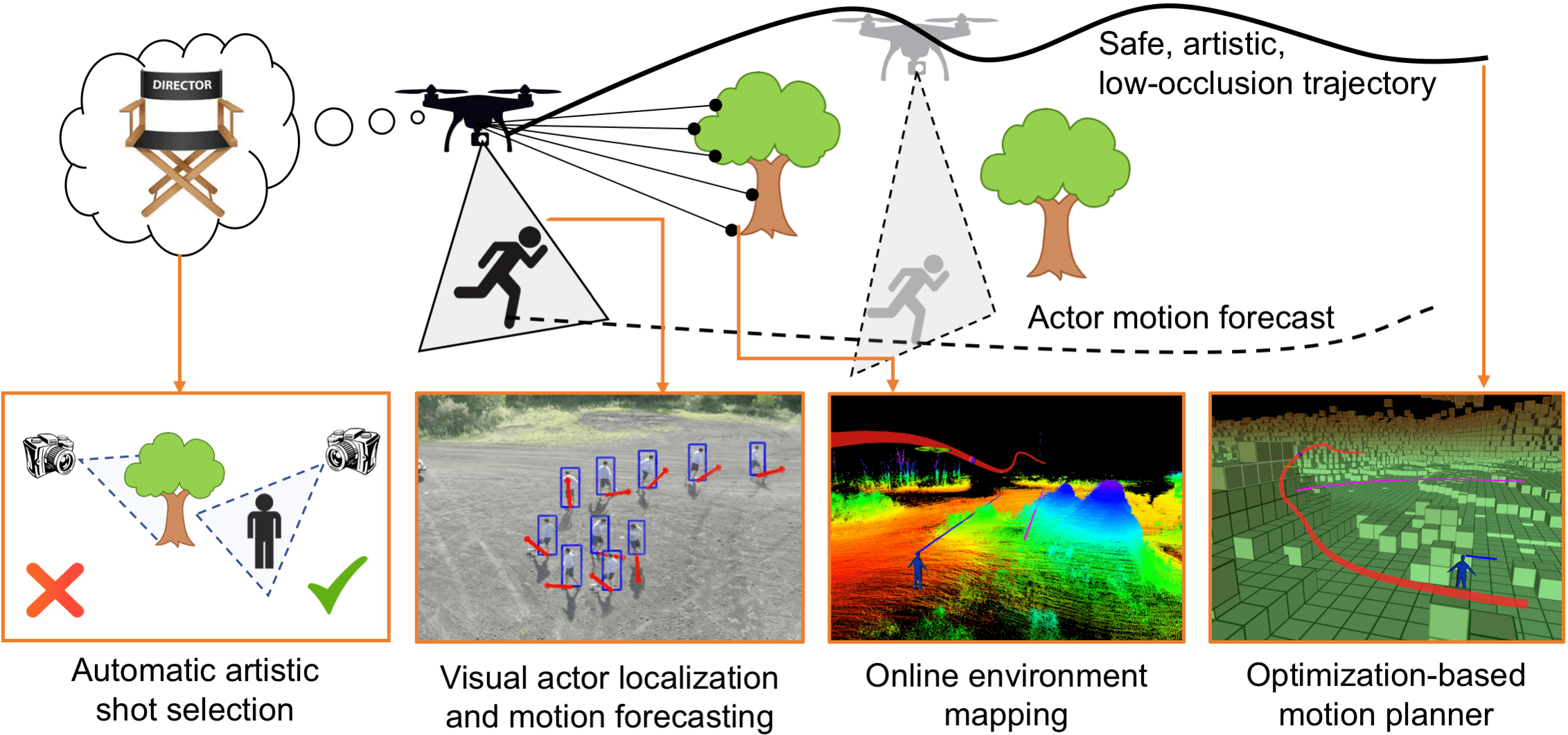
Figure 1: Aerial cinematographer pipeline: the UAV visually detects the actor’s motion using a vision-based localization module, maps the environment with an onboard LiDAR sensor, reasons about artistic guidelines, and plans a smooth, collision-free trajectory while avoiding occlusions.

Manually-operated unmanned aerial vehicles (UAVs) are drastically improving efficiency and productivity in a diverse set of industries and economic activities. In particular, tasks that require dynamic camera viewpoints have been most affected, where the development of small scale UAVs has alleviated the need for sophisticated hardware to manipulate cameras in space. For instance, in the movie industry, drones are changing the way both professional and amateur film-makers can capture shots of actors and landscapes by allowing the composition of aerial viewpoints which are not feasible using traditional devices such as hand-held cameras and dollies [Santamarina-Campos and Segarra-Oña, 2018]. In the sports domain, flying cameras can track fast-moving athletes and accompany dynamic movements [La Bella, 2016]. Furthermore, flying cameras show a largely unexplored potential for tracking subjects of interest in security applications [De-Miguel-Molina, 2018], which are not possible with static sensors.

However, manually-operated UAVs often require multiple expert pilots due to the difficulty of executing all necessary perception and motion planning tasks synchronously: it takes high attention and effort to simultaneously identify the actor(s), predict how the scene is going to evolve, control the UAV, avoid obstacles and reach the desired viewpoints. Hence the need for an autonomous aerial cinematography system.

The distinctive challenge of developing an autonomous aerial cinematography system is the need to tightly couple contextual and geometric threads. Contextual reasoning involves processing camera images to detect the actor, understanding how the scene is going to evolve, and selecting desirable viewpoints. Geometric reasoning considers the 3D configuration of objects in the environment to evaluate the visibility quality of a particular viewpoint and whether the UAV can reach it in a safe manner. Although these two threads differ significantly in terms of sensing modalities, computational representation and computational complexity, both sides play a vital role when addressing the entirety of the autonomous filming problem. In this work we present a complete system that combines both threads in a cohesive and principled manner. In order to develop our autonomous cinematographer, we address several key challenges.

1.1 Challenges

Consider a typical filming scenario in Figure 1. The UAV must overcome several challenges:

Actor pose estimation with challenging visual inputs:

The UAV films a dynamic actor from various angles, therefore it is critical to accurately localize the actor’s position and orientation in a 3D environment. In practice, the use of external sensors such as motion capture systems [Nägeli et al., 2017] and GPS tags [Bonatti et al., 2018, Joubert et al., 2016] for pose estimation is highly impractical; a robust system should only rely on visual localization. The challenge is to deal with all possible viewpoints, scales, backgrounds, lighting conditions, motion blur caused by both the dynamic actor and camera.

Operating in unstructured scenarios:

The UAV flies in diverse, unstructured environments without prior information. In a typical mission, it follows an actor across varying terrain and obstacle types, such as slopes, mountains, and narrow trails between trees or buildings. The challenge is to maintain an online map that has a high enough resolution to reason about viewpoint occlusions and that updates itself fast enough to keep the vehicle safe.

Keep actor visible while staying safe:

In cinematography, the UAV must maintain visibility of the actor for as long as possible while staying safe in a partially known environment. When dealing with dynamic targets, the UAV must anticipate the actor’s motion and reason about collisions and occlusions generated by obstacles in potential trajectories. The challenge of visibility has been explored in previous works in varying degrees of obstacle complexity [Penin et al., 2018, Nägeli et al., 2017, Galvane et al., 2018, Bonatti et al., 2019].

Understanding scene context for autonomous artistic decision-making:

When filming a movie, the director actively selects the camera pose based on the actor’s movement, environment characteristics and intrinsic artistic values. Although humans can make such aesthetic decisions implicitly, it is challenging to define explicit rules to define the ideal artistic choices for a given context.

Making real-time decisions with onboard resources:

Our focus is on unscripted scenarios where shots are decided on the fly; all algorithms must run in real-time with limited computational resources.

1.2 Contributions

Our paper revolves around two key ideas. First, we design differentiable objectives for camera motion that can be efficiently optimized for long time horizons. We architect our system to compute these objectives efficiently online to film a dynamic actor. Second, we apply learning to elicit human artistic preferences in selecting a sequence of shots. Specifically, we offer the following contributions:

1. We propose a method for visually localizing the actor’s position, orientation, and forecasting their future trajectory in the world coordinate frame. We present a novel semi-supervised approach that uses temporal continuity in sequential data for the heading direction estimation problem (Section 5);

2. We propose an incremental signed distance transform algorithm for large-scale real-time environment mapping using a range sensor, e.g., LiDAR (Section 6);

3. We formalize the aerial filming motion planning problem following cinematography guidelines for arbitrary types of shots and arbitrary obstacle shapes. We propose an efficient optimization-based motion planning method that exploits covariant gradients and Hessians of the objective functions for fast convergence (Section 7);

4. We propose a deep reinforcement learning method that incorporates human aesthetic preferences for artistic reasoning to act as an autonomous movie director, considering the current scene context to select the next camera viewpoints (Section 8);

5. We offer extensive quantitative and qualitative performance evaluations both for our integrated system and for each module, both in simulation and field tests (Section 9), along with detailed discussions on experimental lessons learned (Section 10).

This paper builds upon our previous works that each focuses on an individual component of our framework: visual actor detection, tracking and heading estimation [Wang et al., 2019], online environment mapping [Bonatti et al., 2019], motion planning for cinematography [Bonatti et al., 2018], and autonomous artistic viewpoint selection [Gschwindt et al., 2019]. In this paper, for the first time we present a detailed description of the unified architecture (Section 4), provide implementation details of the entire framework, and offer extensive flight test evaluations of the complete system.

2 Problem Definition

The overall task is to control a UAV to film an actor who is moving through an unknown environment. Let $\xi_{q}(t):[0,t_{f}]\rightarrow^{3}\times SO(2)$ be the trajectory of the UAV as a mapping from time to a position and heading, i.e., $\xi_{q}(t)=\{x_{q}(t),y_{q}(t),z_{q}(t),\psi_{q}(t)\}$. Analogously, let $\xi_{a}(t):[0,t_{f}]\rightarrow^{3}\times SO(2)$ be the trajectory of the actor: $\xi_{a}(t)=\{x_{a}(t),y_{a}(t),z_{a}(t),\psi_{a}(t)\}$. In our work, a instantaneous measurement of the actor state $S_{a}:^{3}\times SO(2)$ is obtained using onboard sensors (monocular camera and LiDAR, as seen in Section 5), but external sensors and motion capture systems could also be employed (Section 3). Measurements $S_{a}$ are continuously fed into a prediction module that computes $\xi_{a}$ (Section 5).

The UAV also needs to store a representation of the environment. Let grid $\mathcal{G}:^{3}\rightarrow[0,1]$ be a voxel occupancy grid that maps every point in space to a probability of occupancy. Let $\mathcal{M}:^{3}\rightarrow$ be the signed distance value of a point to the nearest obstacle. Positive signs are for points in free space, and negative signs are for points either in occupied or unknown space, which we assume to be potentially inside an obstacle. During flight the UAV senses the environment with the onboard LiDAR, updates grid $\mathcal{G}$, and then updates $\mathcal{M}$ (more details at Section 6).

We can generically formulate a motion planning problem that aims to minimize a particular cost function $J\left(\xi_{q}\right)$ for cinematography. Within the filming context, this cost function measures jerkiness of motion, safety, environmental occlusion of the actor and shot quality (artistic quality of viewpoints). This cost function depends on the environment $\mathcal{G}$ and $\mathcal{M}$, and on the actor forecast $\xi_{a}$, all of which are sensed on-the-fly. The changing nature of environment and $\xi_{a}$ demands re-planning at a high frequency.

Here we briefly touch upon the four components of the cost function $J\left(\xi_{q}\right)$ (refer to Section 7 for details and mathematical expressions):

1. Smoothness $J_{\mathrm{smooth}}\left(\xi_{q}\right)$: Penalizes jerky motions that may lead to camera blur and unstable flight;

2. Safety $J_{\mathrm{obs}}\left(\xi_{q},\mathcal{M}\right)$: Penalizes proximity to obstacles that are unsafe for the UAV;

3. Occlusion $J_{\mathrm{occ}}\left(\xi_{q},\xi_{a},\mathcal{M}\right)$: Penalizes occlusion of the actor by obstacles in the environment;

4. Shot quality $J_{\mathrm{shot}}\left(\xi_{q},\xi_{a},\Omega_{\mathrm{art}}\right)$: Penalizes poor viewpoint angles and scales that deviate from the desired artistic guidelines, given by the set of parameters $\Omega_{\mathrm{art}}$.

In its simplest form, we can express $J\left(\xi_{q}\right)$ as a linear composition of each individual cost, weighted by scalars $\lambda_{i}$. The objective is to minimize $J\left(\xi_{q}\right)$ subject to initial boundary constraints $\xi_{q}(0)$. The solution $\xi_{q}^{*}$ is then tracked by the UAV:

$$J\left(\xi_{q}\right) =\begin{bmatrix}1&\lambda_{1}&\lambda_{2}&\lambda_{3}\end{bmatrix}\begin{bmatrix}J_{\mathrm{smooth}}\left(\xi_{q}\right)\\ J_{\mathrm{obs}}\left(\xi_{q},\mathcal{M}\right)\\ J_{\mathrm{occ}}\left(\xi_{q},\xi_{a},\mathcal{M}\right)\\ J_{\mathrm{shot}}\left(\xi_{q},\xi_{a},\Omega_{art}\right)\end{bmatrix}$$ (1)

$$\xi_{q}^{*} =\underset{\xi_{q}}{\operatorname*{arg\,min}}\quad J\left(\xi_{q}\right),\quad\text{s.t.}\;\xi_{q}(0)=\{x_{0},y_{0},z_{0},\psi_{0}\}$$

We describe in Section 7 how (1) is solved. The parameters $\Omega_{\mathrm{art}}$ of the shot quality term $J_{\mathrm{shot}}$ are usually specified by the user prior to takeoff, and assumed constant throughout flight. For instance, based on the terrain characteristics and the type of motion the user expects the actor to do, they may specify a frontal or circular shot with a particular scale to be the best artistic choice for that context. Alternatively, $\Omega_{\mathrm{art}}$ can change dynamically, either by user’s choice or algorithmically.

A dynamically changing $\Omega_{\mathrm{art}}$ leads to a new challenge: the UAV must make choices that maximize the artistic value of the incoming visual feed. As explained further in Section 8, artistic choices affect not only the immediate images recorded by the UAV. By changing the positioning of the UAV relative to the subject and obstacles, current choices influence the images captured in future time steps. Therefore, the selection of $\Omega_{\mathrm{art}}$ needs to be framed as a sequential decision-making process.

Let $v_{t}=\{I_{1},I_{2},...,I_{k}\}$ be a sequence of $k$ observed images captured by the UAV during time step $t$ between consecutive artistic decisions. Let $R_{\mathrm{art}}(v_{t})$ be the user’s implicit evaluation reward based on the observed the video segment $v_{t}$. The user’s choice of an optimal artistic parameter sequence $\{\Omega_{1}^{*},\Omega_{2}^{*},...,\Omega_{n}^{*}\}$ can be interpreted as an optimization of the following form:

$$\{\Omega_{1}^{*},\Omega_{2}^{*},...,\Omega_{n}^{*}\}=\underset{\{\Omega_{1},\Omega_{2},...,\Omega_{n}\}}{\operatorname*{arg\,max}}\quad\sum_{t}R_{\mathrm{art}}(v_{t})$$ (2)

The optimization from Equation 2 is usually left up to the UAV operator’s experience and intuition. In Section 8, we detail a novel method for implicitly learning the selection of artistic parameters depending on the scene’s context.

3 Related Work

Our work exploits synergies at the confluence of several domains of research to develop an aerial cinematography platform that can follow dynamic targets in unstructured environments using onboard sensors and computing power. Next, we describe related works in different areas that come together under the problem definition described in Section 2.

Virtual cinematography:

Camera control in virtual cinematography has been extensively examined by the computer graphics community as reviewed by [Christie et al., 2008]. These methods typically reason about the utility of a viewpoint in isolation, follow artistic principles and composition rules [Arijon, 1976, Bowen and Thompson, 2013] and employ either optimization-based approaches to find good viewpoints or reactive approaches to track the virtual actor. The focus is typically on through-the-lens control where a virtual camera is manipulated while maintaining focus on certain image features [Gleicher and Witkin, 1992, Drucker and Zeltzer, 1994, Lino et al., 2011, Lino and Christie, 2015]. However, virtual cinematography is free of several real-world limitations such as robot physics constraints and assumes full knowledge of the environment.

Several works analyse the choice of which viewpoint to employ for a particular situation. For example, in [Drucker and Zeltzer, 1994], the researchers use an A* planner to move a virtual camera in pre-computed indoor simulation scenarios to avoid collisions with obstacles in 2D. More recently, we find works such as [Leake et al., 2017] that post-processes videos of a scene taken from different angles by automatically labeling features of different views. The approach uses high-level user-specified rules which exploit the labels to automatically select the optimal sequence of viewpoints for the final movie. In addition, [Wu et al., 2018] help editors by defining a formal language of editing patterns for movies.

Autonomous aerial cinematography:

There is a rich history of work in autonomous aerial filming. For instance, several works focus on following user-specified artistic guidelines [Joubert et al., 2016, Nägeli et al., 2017, Galvane et al., 2017, Galvane et al., 2018] but often rely on perfect actor localization through a high-precision RTK GPS or a motion-capture system. Additionally, although the majority of work in the area deals with collisions between UAV and actors[Nägeli et al., 2017, Joubert et al., 2016, Huang et al., 2018a], they do not factor in the environment for safety considerations. While there are several successful commercial products, they too have certain limitations such as operating in low speed and low clutter regimes (e.g. DJI Mavic [DJI, 2018]) or relatively short planning horizons (e.g. Skydio R1 [Skydio, 2018]). Even our previous work [Bonatti et al., 2018], despite handling environmental occlusions and collisions, assumes a prior elevation map and uses GPS to localize the actor. Such simplifications impose restrictions on the diversity of scenarios that the system can handle.

Several contributions on aerial cinematography focus on keyframe navigation. [Roberts and Hanrahan, 2016, Joubert et al., 2015, Gebhardt et al., 2018, Gebhardt et al., 2016, Xie et al., 2018] provide user interface tools to re-time and connect static aerial viewpoints to provide smooth and dynamically feasible trajectories, as well as a visually pleasing images. [Lan et al., 2017] use key-frames defined on the image itself instead of world coordinates.

Other works focus on tracking dynamic targets, and employ a diverse set of techniques for actor localization and navigation. For example, [Huang et al., 2018a, Huang et al., 2018b] detect the skeleton of targets from visual input, while others approaches rely on off-board actor localization methods from either motion-capture systems or GPS sensors [Joubert et al., 2016, Galvane et al., 2017, Nägeli et al., 2017, Galvane et al., 2018, Bonatti et al., 2018]. These approaches have varying levels of complexity: [Bonatti et al., 2018, Galvane et al., 2018] can avoid obstacles and occlusions with the environment and with actors, while other approaches only handle collisions and occlusions caused by actors. In addition, in our latest work [Bonatti et al., 2019] we made two important improvements on top of [Bonatti et al., 2018] by including visual actor localization and online environment mapping.

Specifically on the motion planning side, we note that different UAV applications can influence the choice of motion planning algorithms. The main motivation is that different types of planners can exploit specific properties and guarantees of the cost functions. For example, sampling-based planners [Kuffner and LaValle, 2000, Karaman and Frazzoli, 2011, Elbanhawi and Simic, 2014] or search-based planners [LaValle, 2006, Aine et al., 2016] should ideally use fast-to-compute costs so that many different states can be explored during search in high-dimensional state spaces. Other categories of planners, based on trajectory optimization [Ratliff et al., 2009a, Schulman et al., 2013], usually require cost functions to be differentiable to the first or higher orders. We also find hybrid methods that make judicious use of optimization combined with search or sampling [Choudhury et al., 2016, Luna et al., 2013].

Furthermore, different systems present significant differences in onboard versus off-board computation. We summarize and compare contributions from past works in Table LABEL:tab:related_work. It is important to notice that none of the previously published approaches provides a complete solution to the generic aerial cinematography problem using only onboard resources.

Table 1: Comparison of dynamic aerial cinematography systems. Notes: i) [Huang et al., 2018a] define artistic selection as the viewpoint that maximizes the projection of the actor on the image; ii) [Bonatti et al., 2018] localize the actor visually only for control of the camera gimbal, but use GPS to obtain the actor’s position in global coordinates for planning; iii) Cells marked with “Actor” for occlusion and obstacle avoidance mean that those approaches only take into account the actors in the scene as ellipsoidal obstacles, and disregard other objects.

0cmReference	1.8cmOnline
art. selec.

& 1.1cmOnline map 0.6cmActor localiz. 1.3cmOnboard comp. 0cmAvoids occl. 0cmAvoids obst. 0.9cmOnline plan [Galvane et al., 2017] $\times$ $\times$ $\times$ $\times$ $\times$ $\times$ ✓ [Joubert et al., 2016] $\times$ $\times$ $\times$ $\times$ $\times$ Actor ✓ [Nägeli et al., 2017] $\times$ $\times$ $\times$ $\times$ Actor Actor ✓ [Galvane et al., 2018] $\times$ $\times$ $\times$ $\times$ ✓ ✓ ✓

[Huang et al., 2018b] $\times$ $\times$ ✓ ✓ $\times$ Actor ✓ [Huang et al., 2018a] Actor proj. $\times$ $\checkmark$ ✓ $\times$ Actor ✓ [Bonatti et al., 2018] $\times$ $\times$ Vision ✓ ✓ ✓ ✓ [Bonatti et al., 2019] $\times$ ✓ ✓ ✓ ✓ ✓ ✓       Ours ✓ ✓ ✓ ✓ ✓ ✓ ✓

Making artistic choices autonomously:

A common theme behind all the work presented so far is that a user must always specify which kind of output they expect from the system in terms of artistic behavior. This behavior is generally expressed in terms of the set of parameters $\Omega_{art}$, and relates to different shot types, camera angles and angular speeds, type of actor framing, etc. If one wishes to autonomously specify artistic choices, two main points are needed: a proper definition of a metric for artistic quality of a scene, and a decision-making agent which takes actions that maximize this quality metric, as explained in Equation 2.

Several works explore the idea of learning a beauty or artistic quality metric directly from data. [Karpathy, 2015] learns a measure for the quality of selfies; [Fang and Zhang, 2017] learn how to generate professional landscape photographs; [Gatys et al., 2016] learn how to transfer image styles from paintings to photographs.

On the action generation side, we find works that have exploited deep reinforcement learning [Mnih et al., 2015] to train models that follow human-specified behaviors. Closest to our work, [Christiano et al., 2017] learns behaviors for which hand-crafted rewards are hard to specify, but which humans find easy to evaluate.

Our work, as described in Section 8, brings together ideas from all the aforementioned areas to create a generative model for shot type selection in aerial filming drones which maximizes an artistic quality metric.

Online environment mapping:

Dealing with imperfect representations of the world becomes a bottleneck for viewpoint optimization in physical environments. As the world is sensed online, it is usually incrementally mapped using voxel occupancy maps [Thrun et al., 2005]. To evaluate a viewpoint, methods typically raycast on such maps, which can be very expensive [Isler et al., 2016, Charrow et al., 2015]. Recent advances in mapping have led to better representations that can incrementally compute the truncated signed distance field (TSDF) [Newcombe et al., 2011, Klingensmith et al., 2015], i.e. return the distance and gradient to nearest object surface for a query. TSDFs are a suitable abstraction layer for planning approaches and have already been used to efficiently compute collision-free trajectories for UAVs [Oleynikova et al., 2016, Cover et al., 2013].

Visual target state estimation:

Accurate object state estimation with monocular cameras is critical for many robot applications, including autonomous aerial filming. Two key problems in target state estimation include detecting objects and their orientation.

Deep learning based techniques have achieved remarkable progress in the area of 2D object detection, such as YOLO (You Only Look Once) [Redmon et al., 2016], SSD (Single Shot Detector) [Liu et al., 2016b] and Faster R-CNN method [Ren et al., 2015]. These methods use convolutional neural networks (CNNs) for bounding box regression and category classification. They requires powerful GPUs, and cannot achieve real-time performance when deployed to the onboard platform. Another problem with off-the-shelf models trained on open datasets is that they do not generalize well to the areal filming scenario due to mismatches in data distribution due to angles, lighting, distances to actor and motion blur. Later in Section 5 we present our approach for obtaining a real-time object detector for our application.

Another key problem in the actor state estimation for aerial cinematography is estimating the heading direction of objects in the scene. Heading direction estimation (HDE) has been widely studied especially in the context of humans and cars as target objects. There have been approaches that attach sensors including inertial sensors and GPS to the target object to obtain the object’s [Liu et al., 2016a, Deng et al., 2017][Vista et al., 2015] heading direction. While these sensors provide reliable and accurate estimation, it is highly undesirable for the target actor to carry these extra sensors. Thus, we primarily focus on vision-based approaches for our work that don’t require the actor to carry any additional equipment.

In the context of Heading Direction Estimation using visual input, there have been approaches based on classical machine learning techniques. Based on a probabilistic framework, [Flohr et al., 2015] present a joint pedestrian head and body orientation estimation method, in which they design a HOG based linear SVM pedestrian model. Learning features directly from data rather than handcrafting them has proven more successful, especially in the domain of computer vision. We therefore leverage learning based approaches that ensure superior generalizability and improved robustness.

Deep learning based approaches have been successfully applied to the area of 2D pose estimation [Toshev and Szegedy, 2014, Cao et al., 2017] which is a related problem. However, the 3D heading direction cannot be trivially recovered from 2D points because the keypoint’s depth remains undefined and ambiguous. Also, these approaches are primarily focused on humans and don’t address other objects including cars.

There are fewer large scale datasets for 3D pose estimation [Ionescu et al., 2014, Raman et al., 2016, Liu et al., 2013, Geiger et al., 2013] and the existing ones generalize poorly to our aerial filming task, again due to mismatch in the data distribution. Thus, we look for approaches that can be applied in limited labeled data setting. The limited dataset constraint is common in many robotics applications, where the cost of acquiring and labeling data is high. Semi-supervised learning (SSL) is an active research area in this domain. However, most of the existing SSL works are primarily focused on classification problems [Weston et al., 2012, Hoffer and Ailon, 2016, Rasmus et al., 2015, Dai et al., 2017], which assume that different classes are separated by a low-density area and easy to separate in high dimensional space. This assumption is not directly applicable to regression problems.

In the context of cinematography, temporal continuity can be leveraged to formulate a semi-supervised regression problem. [Mobahi et al., 2009] developed one of the first approaches to exploit temporal continuity in the context of deep convolutional neural networks. The authors use video temporal continuity over the unlabeled data as a pseudo-supervisory signal and demonstrate that this additional signal can improve object recognition in videos from the COIL-100 dataset [Nene et al., 1996]. There are other works that learn feature representations by exploiting temporal continuity [Zou et al., 2012, Goroshin et al., 2015, Stavens and Thrun, 2010, Srivastava et al., 2015, Wang and Gupta, 2015]. [Zou et al., 2012] included the video temporal constraints in an autoencoder framework and learn invariant features across frames. [Wang and Gupta, 2015] designed a Siamese-triplet network which can be trained in an unsupervised manner with a large amount of video data, and showed that the unsupervised visual representation can achieve competitive performance on various tasks, compared to its ImageNet-supervised counterpart. Inspired by these approaches, our recent work [Wang et al., 2019] aims to improve the learning of a regression model from a small labeled dataset by leveraging unlabeled video sequences to enforce temporally smooth output predictions.

After the target’s location and heading direction is estimated on the image plane, we can project it onto the world coordinates and use different methods to estimate the actor’s future motion. Motion forecast methods can range from filtering methods such as Kalman filters and extended Kalman filters [Thrun et al., 2005], which are based solely on the actor’s dynamics, to more complex methods that take into account environmental features as well. As an example of the latter, [Urmson et al., 2008] use traditional motion planner with handcrafted cost functions for navigation among obstacles, and [Zhang et al., 2018] use deep inverse reinforcement learning to predict the future trajectory distribution vehicles among obstacles.

4 System Overview

In this section we detail the design hypotheses (Subsec. 4.1) that influenced the system architecture layout (Subsec. 4.2), as well as our hardware (Subsec. 4.3) and simulation (Subsec. 4.4) platforms.

4.1 Design Hypotheses

Given the application challenges (Subsec. 1.1) and problem definition (Sec. 2), we defined three key hypotheses to guide the layout of the system architecture for the autonomous aerial cinematography task. These hypotheses serve as high-level principles for our choice of sub-systems, sensors and hardware. We evaluate the hypotheses later in Section 9, where we detail our simulation and field experiments.

This is a fundamental assumption and a necessary condition for development of real-world aerial cinematography systems that do not rely on ground-truth data from off-board sensors. We hypothesize our system can deal with noisy measurements and extract necessary actor and obstacle information for visual actor localization, mapping and planning.

Decoupling gimbal control from motion planning improves real-time performance and robustness to noisy actor measurements. We assume that an independent 3-DOF camera pose controller can compensate for noisy actor measurements. We expect advantages in two sub-systems: (i) the motion planner can operate faster and with a longer time horizon due to the reduced trajectory state space, and (ii) visual tracking will be more precise because the controller uses direct image feedback instead of a noisy estimate of the actor’s location. We use a gimbaled camera with 3-DOF control, which is a reasonable requirement given today’s UAV and camera technology.

Analogous to the role of a movie director, the artistic intent sub-system should provide high-level guidelines for camera positioning, but not interfere directly on low-level controls. We hypothesize that a hierarchical structure to guide artistic filming behavior employing high-level commands is preferable to an end-to-end low-level visio-motor policy because: (i) it’s easier to ensure overall system safety and stability by relying on more established motion planning techniques, and (ii) it’s more data-efficient and easier to train a high-level decision-making agent than an end-to-end low-level policy.

4.2 System Architecture

Taking into account the design hypotheses, we outline the software architecture in Figure 2. The system consists of 4 main modules: Vision, Mapping, Planning and Artistic Shot Selection. The four modules run in parallel, taking in camera, LiDAR and GPS inputs to output gimbal and flight controller commands for the UAV platform.

Vision (Section 5):

The module takes in monocular images to compute a predicted actor trajectory for the Shot Selection and Planning Module. Following Hyp. 2, the vision module also controls the camera gimbal independently of the planning module.

Mapping (Section 6):

The module registers the accumulated LIDAR point cloud and outputs different environment representations: obstacle height map for raycasting and shot selection, and truncated signed distance transform (TSDT) map for the motion planner.

Artistic Shot Selection (Section 8):

Following Hyp. 3 the module acts as an artistic movie director and defines high-level inputs for the motion planner defining the most aesthetic shot type (left, right, front, back) for a given scene context, composed of actor trajectory and obstacle locations.

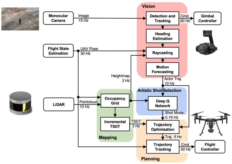
Figure 2: The system consists of 4 main modules running in parallel: Vision, Mapping, Planning and Artistic Shot Selection. The system takes in visual, LiDAR and GPS inputs to output gimbal and flight controller commands.

Planning (Section 7):

The planning module takes in the predicted actor trajectory, TSDT map, and the desired artistic shot mode to compute a trajectory that balances safety, smoothness, shot quality and occlusion avoidance. Using the UAV pose estimate, the module outputs velocity commands for the UAV to track the computed trajectory.

4.3 Hardware

Our base platform is the DJI M210 quadcopter, shown in Figure 3. The UAV fuses GPS, IMU and compass for state estimation, which can be accessed via DJI’s SDK. The M210 has a maximum payload capacity of $2.30$ kg , which limits our choice of batteries and onboard computers and sensors.

Our payload is composed of (weights are summarized in Table 2):

• DJI TB50 Batteries, with maximum flight time of $13$ minutes at full payload;

• DJI Zenmuse X4S gimbaled camera, whose 3-axis gimbal can be controlled independently of the UAV’s motion with angular precision of $\pm 0.01^{\circ}$, and counts with a vibration-dampening structure. The camera records high-resolution videos, up to 4K at 60 FPS;

• NVIDIA Jetson TX2 with Astro carrier board. 8 GB of RAM, 6 CPU cores and 256 GPU cores for onboard computation;

• Velodyne Puck VLP-16 Lite LiDAR, with $\pm 15^{\circ}$ vertical field of view and $100$ m max range.

Table 2: System and payload weights.

Component	Weight (kg)
DJI M210	2.80
DJI Zenmuse X4S	0.25
DJI TB 50 Batteries $\times$ 2	1.04
NVIDIA TX2 w/ carrier board	0.30
VLP-16 Lite	0.59
Structure Modifications	0.63
Cables and connectors	0.28
Total:	5.89 $\leq$ 6.14 (maximum takeoff weight 1)

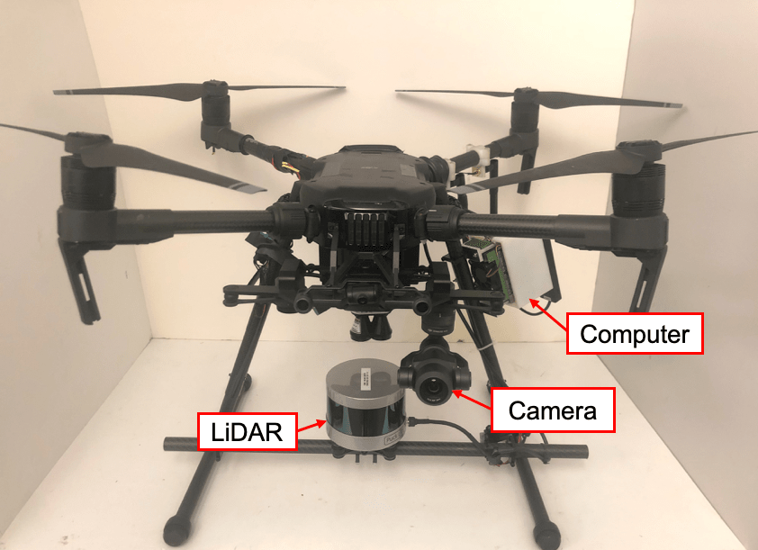
Figure 3: System hardware: DJI M210 drone equipped with Nvidia TX2 computer, Velodyne VLP-16 Puck Lite LiDAR and Zenmuse X4S camera gimbal.

4.4 Photo-realistic Simulation Platform

We use the Microsoft AirSim simulation platform [Shah et al., 2018] to test our framework and to collect training data for the shot selection module, as explained in detail in Section 8. Airsim offers a high-fidelity visual and physical simulation for quadrotors and actors (such as humans and cars), as shown in Figure 4. We built a custom ROS [Quigley et al., 2009] interface for the simulator, so that our system can switch between the simulation and the real drone seamlessly. All nodes from the system architecture are written in C++ and Python languages, and communicate using the ROS framework.

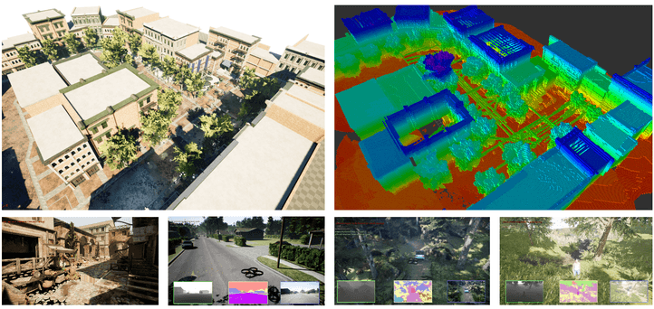
Figure 4: Simulation platform: Airsim combines a physics engine with photo-realistic renderings of various environments and actors (human and vehicles). Here we show the urban and forest environments we used for testing our framework. We build a point cloud and an occupancy map in the simulation. The simulation provides ground truth data for the actor’s pose, which is used to evaluate the performance of the vision pipeline.

5 Visual Actor Localization and Heading Estimation

The vision module is responsible for two critical roles in the system: to estimate the actor’s future trajectory and to control the camera gimbal to keep the actor within the frame. Figure 5 details the four main sub-modules: actor detection and tracking, heading direction angle estimation, global position ray-casting, and finally a filtering stage for trajectory forecasting. Next, we detail each sub-module.

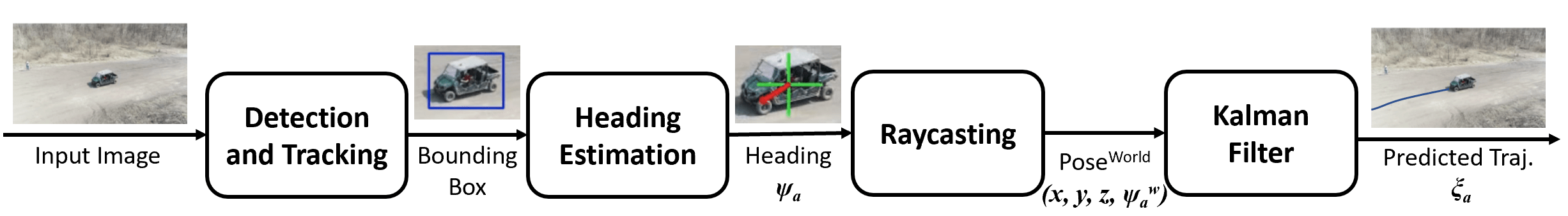
Figure 5: Vision sub-system. We detect and track the actor’s bounding box, estimate its heading, and project its pose to world coordinates. A Kalman Filter predicts the actor’s forecasted trajectory $\xi_{a}$.

5.1 Detection and Tracking

As we discussed in Section 3, the state-of-the-art object detection methods require large computational resources, which are not available on our onboard platform, and do not perform well in our scenario due to the data distribution mismatch. Therefore, we develop two solutions: first, we build a custom network structure and train it on both the open and context-specific datasets in order to improve speed and accuracy; second, we combine the object detector with a real-time tracker for stable performance.

The deep learning based object detectors are composed of a feature extractor followed by a classifier or regressor. Different feature extractors could be used in each detector to balance efficiency and accuracy. Since the onboard embedded GPU is less powerful, we can only afford feature extractor with relatively fewer layers. We compare several lightweight publicly available trained models for people detection and car detection.

Due to good real-time inference speed and low memory usage, we combine the MobileNet [Howard et al., 2017] for feature extraction and the Faster-RCNN [Ren et al., 2015] architecture. Our feature extractor consists of 11 depth-wise convolutional modules, which contains 22 convolutional layers. Following the Faster-RCNN structure, the extracted feature then goes to a two-stage detector, namely a region proposal stage and a bounding box regression and classification stage. While the size of the original Faster-RCNN architecture with VGG is 548 MB, our custom network’s is 39 MB, with average inference time of $300$ ms.

The distribution of images in the aerial filming task differs significantly from the usual images found in open accessible datasets, due to highly variable relative yaw and tilt angles to the actors, large distances, varying lighting conditions and heavy motion blur. Figure 6 displays examples of challenging situations faced in the aerial cinematography problem. Therefore, we trained our network with images from two sources: a custom dataset of 120 challenging images collected from field experiments, and images from the COCO [Lin et al., 2014] dataset, in a 1:10 ratio. We limited the detection categories only to person, car, bicycle, and motorcycle, which are object types that commonly appear as actors in aerial filming.

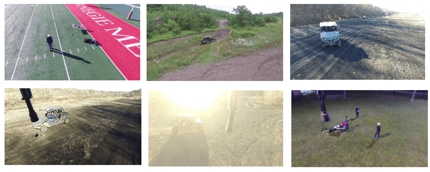
Figure 6: Examples of challenging images for actor detection in the aerial filming task. Large relative tilt angles to the ground, variable lighting, large distance to actor and heavy motion blur make bounding box detection harder than in images from open datasets.

The detection module receives the main camera’s monocular image as inputs, and outputs a bounding box. We use this initial bounding box to initialize a template tracking process, and re-initialize detection whenever the tracker’s confidence falls below acceptable limits. We adopt this approach, as opposed to detecting the actor in every image frame, because detection is a computationally heavy process, and the high rate of template tracking provides more stable measurements for subsequent calculations. We use Kernelized Correlation Filters [Henriques et al., 2015] to track the template over the next incoming frames.

As mentioned in Section 4, we actively control camera gimbal independently of the UAV’s motion to maintain visibility of the target. We use a PD controller to frame the actor on the desired screen position, following the commanded artistic principles from the operator. Typically, the operator centers the target on the middle of the image space, or uses visual composition rules such as the rule of thirds [Bowen and Thompson, 2013], as seen on Figure 7.

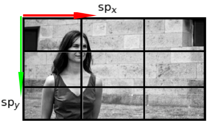
Figure 7: Desired screen position of the actor projection, defined by parameters: $\mathrm{sp_{x}},\mathrm{sp_{y}}\in[0,1]$. Typically the user uses one of the thirds of the screen to set the actor’s position, or centers the actor on the frame [Bowen and Thompson, 2013].

5.2 Heading Estimation

When filming a moving actor, heading direction estimation (HDE) plays a central role in motion planning. Using the actor’s heading information, the UAV can position itself within the desired shot type determined by the user’s artistic objectives, e.g: back, front, left and right side shots, or within any other desired relative yaw angle.

Estimating the heading of people and objects is also an active research problem in many other applications, such as pedestrian collision risk analysis [Tian et al., 2014], human-robot interaction [Vázquez et al., 2015] and activity forecasting [Kitani et al., 2012]. Similar to challenges in bounding box detection, models obtained in other datasets do not easily generalize to the aerial filming task, due to a mismatch in the types of images from datasets to our application. In addition, when the trained model is deployed on the UAV, errors is compounded because the HDE relies on a imperfect object detection module, increasing the mismatch [Ristani et al., 2016, Geiger et al., 2013].

No current dataset satisfies our needs for aerial HDE, creating the need for us to create a custom labeled dataset for our application. As most deep learning approaches, training a network is a data-intensive process, and manually labeling a large enough dataset for conventional supervised learning is a laborious and expensive task. The process is further complicated as multiple actor types such as people, cars and bicycles can appear in footages.

These constraints motivated us to formulate a novel semi-supervised algorithm for the HDE problem [Wang et al., 2019]. To drastically reduce the quantity of labeled data, we leverage temporal continuity in video sequences as an unsupervised signal to regularize the model and achieve better generalization. We apply the semi-supervised algorithm in both training and testing phases, drastically increasing inference performance, and show that by leveraging unlabeled sequences, the amount of labeled data required can be significantly reduced.

5.2.1 Defining the loss for temporal continuity

We define the pose of the actor as a vector $[x,y,z,\psi_{a}^{w}]$ on the ground surface. In order to estimate the actor’s heading direction in the world frame $\psi_{a}^{w}$, we first predict the actor’s heading $\psi_{a}$ in the image frame, as shown in Figure 8. Once $\psi_{a}$ is estimated, we project this direction onto the world frame coordinates using the camera’s intrinsic and extrinsic matrices.

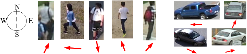
Figure 8: Example of actor bounding boxes and their respective heading angles $\psi_{a}$ in image space. Given the images, our objective is to predict the heading direction, shown as red arrows.

The HDE module outputs the estimated heading angle $\psi_{a}$ in image space. Since $\psi_{a}$ is ambiguously defined at the frontier between $-\pi$ and $\pi$, we define the inference as a regression problem that outputs two continuous values: $[\cos(\psi_{a}),\sin(\psi_{a})]$. This avoids model instabilities during training and inference.

We assume access to a relatively small labeled dataset $D=\{(x_{i},y_{i})\}_{i=0}^{n}$, where $x_{i}$ denotes input image, and $y_{i}=[cos(\psi_{i}),sin(\psi_{i})]$ denotes the angle label. In addition, we assume access to a large unlabeled sequential dataset $U=\{q_{j}\}_{j=0}^{m}$, where $q_{j}=\{x_{0},x_{1},...,x_{t}\}$ is a sequence of temporally-continuous image data.

The HDE module’s main objective is to approximate a function $y=f(x)$, that minimizes the regression loss on the labeled data $\sum_{(x,y)\in{D}}L_{l}(x_{l},y_{l})=\sum_{(x,y)\in{D}}||y_{i}-f(x_{i})||^{2}$. One intuitive way to leverage unlabeled data is to add a constraint that the output of the model should not have large discrepancies over a consecutive input sequence. Therefore, we train the model to jointly minimize the labeled loss $L_{l}$ and some continuity loss $L_{u}$. We minimize the combined loss:

$$L_{tot}=\min{\sum_{(x_{l},y_{l})\in{L}}L_{l}(x_{l},y_{l})+\lambda\sum_{q_{u}\in{U}}{L_{u}(q_{u})}}$$ (3)

We define the unsupervised loss using the idea that samples closer in time should have smaller differences in angles than samples further away in time. A similar continuity loss is also used by [Wang and Gupta, 2015] when training an unsupervised feature extractor:

$$L_{u}(q_{u}) =\sum_{x_{1},x_{2},x_{3}}\max[0,D(x_{1},x_{2};f)-D(x_{1},x_{3};f)],$$ (4)

where: $$D(x_{1},x_{2};f)=||f(x_{1})-f(x_{2})||_{2},$$

and: $$x_{1},x_{2},x_{3}\in{q_{u}}$$

5.2.2 Network structure

For lower memory usage and faster inference time in the onboard computer, we design a compact CNN architecture based on MobileNet [Howard et al., 2017]. The input to the network is a cropped image of the target’s bounding box, outputted by the detection and tracking modules. The cropped image is padded to a square shape and resized to 192 x 192 pixels. After the 10 group-wise and point-wise convolutional blocks from the original MobileNet architecture, we add another convolutional layer and a fully connected layer that output two values representing the cosine and sine values of the angle. Figure 9 illustrates the architecture.

During each training iteration, one shuffled batch of labeled data and one sequence of unlabeled data are passed through the network. The labeled loss and unlabeled losses are computed and backpropagated through the network.

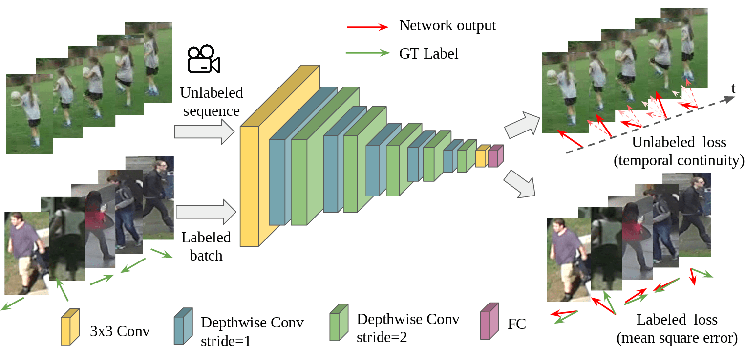
Figure 9: Our network architecture for predicting the actor’s heading direction. We use a Mobilenet-based feature extractor followed by a convolutional layer and a fully connected layer to regress to angular values. The network is trained using both labeled and unsupervised losses.

5.2.3 Cross-dataset semi-supervised fine-tuning

Due to data distribution mismatch between the aerial cinematography task and open datasets, we train our network on a combination of images from both sources. Later in Subsection 9.2 we evaluate the impact of fine-tuning the training process with unsupervised videos from our application.

5.3 Ray-casting

The ray-casting module convert the detection/tracking and HDE results from image space to coordinates and heading in the world frame $[x,y,z,\psi_{a}^{w}]$. Given the actor’s bounding box, we project its center-bottom point onto a height map of the terrain, provided by the mapping module. The intersection of this line with the height map provides the $[x,y,z]$ location of the actor.

Assuming that the camera gimbal’s roll angle is fixed at zero degrees by the active gimbal controller, we can directly obtain the actor’s heading direction on the world frame $\psi_{a}^{w}$ by transforming the heading $\psi$ from the image space with the camera’s extrinsic matrix in world coordinates.

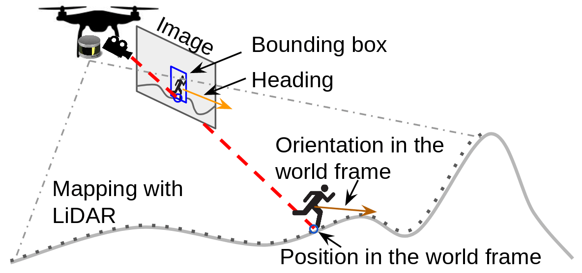
Figure 10: Raycasting module uses the actor’s bounding box, estimated heading angle, environment height map and camera matrices to obtain pose of actor in the world frame $[x,y,z,\psi_{a}^{w}]$.

5.4 Motion Forecasting

Given a sequence of actor poses in the world coordinates, we estimate the actor’s future trajectory based on motion models. The motion planner later uses the forecast to plan non-myopically over long time horizons.

We use two different motion models depending on the actor types. For people, we apply a linear Kalman filter with a two-dimensional motion model. Since a person’s movement direction can change drastically, we use no kinematic constraints applied to the motion model, and just assume constant velocity. We assume no control inputs for state $[x,y,\dot{x},\dot{y}]$ in the prediction step, and use the next measurement of $[x,y,z]$ in the correction step. When forecasting the motion of cars and bicycles we apply an extended Kalman filter with a kinematic bicycle model. For both cases we use a $10$ s horizon for prediction.

6 Online Environment Mapping

As explained in Section 2, the motion planner requires signed distance values $\mathcal{M}$ to solve the optimization problem that results in the final UAV trajectory. The main role of the mapping subsystem described here is to register LiDAR points from the onboard sensor, update the occupancy grid $\mathcal{G}$, and incrementally update the signed distance $\mathcal{M}$.

6.1 LiDAR Registration

During our filming operation, we receive approximately $300,000$ points per second from the laser sensor mounted at the bottom of the aircraft. We register the points in the world coordinate system using a rigid body transform between the sensor and the aircraft plus the UAV’s state estimation, which fuses GPS, barometer, internal IMUs and accelerometers. For each point we also store the corresponding sensor coordinate, which is used for the occupancy grid update.

LiDAR points can be categorized either as hits, which represent successful laser returns within the maximum range of $100$ m, or as misses, which represent returns that are either non-existent, beyond the maximum range, or below a minimum sensor range. We filter all expected misses caused by reflections from the aircraft’s own structure. Finally, we probabilistically update all voxels from $\mathcal{G}$ between the sensor and its LiDAR returns, as described in Subsection 6.2.

6.2 Occupancy Grid Update

The mapping subsystem holds a rectangular grid that stores the likelihood that any cell in space is occupied. In this work we use a grid size of $250\times 250\times 100$ m, with $1$ m square voxels that store an $8$-bit integer value between $0-255$ as the occupancy probability, where $0$ is the limit for a fully free cell, and $255$ is the limit for a fully occupied cell. All cells are initialized as unknown, with value of $127$.

Algorithm 1 covers the grid update process. The inputs to the algorithm are the sensor position $p_{\mathrm{sensor}}$, the LiDAR point $p_{\mathrm{point}}$, and a flag is_hit that indicates whether the point is a hit or miss. The endpoint voxel of a hit will be updated with log-odds value $l_{\mathrm{occ}}$, and all cells in between sensor and endpoint will be updated by subtracting value $l_{\mathrm{free}}$. We assume that all misses are returned as points at the maximum sensor range, and in this case only the cells between endpoint and sensor are updated $l_{\mathrm{free}}$.

As seen in Algorithm 1, all voxel state changes to occupied or free are stored in lists $V^{\mathrm{change}}_{\mathrm{occ}}$ and $V^{\mathrm{change}}_{\mathrm{free}}$. State changes are used for the signed distance update, as explained in Subsection 6.3.

Initialize $V^{\mathrm{change}}_{\mathrm{occ}}$, $V^{\mathrm{change}}_{\mathrm{free}}$ $\triangleright$ list of changed voxels

 Initialize $l_{\mathrm{free}}$, $l_{\mathrm{occ}}$ $\triangleright$ log-odds probabilistic updates

1 for each voxel $v$ between $p_{\mathrm{sensor}}$ and $p_{\mathrm{point}}$ do

2       $v\leftarrow v-l_{\mathrm{free}}$;

3       if $v$ was occupied or unknown and now is free then

4             Append($v$, $V^{\mathrm{change}}_{\mathrm{free}}$);

5             for each unknown neighbor $v_{\mathrm{unk}}$ of $v$ do

6                   Append($v_{\mathrm{unk}}$, $V^{\mathrm{change}}_{\mathrm{occ}}$)

7             end for

8            

9       end if

10      if $v$ is the endpoint and is_hit is true then

11             $v\leftarrow v+l_{\mathrm{occ}}$;

12             if $v$ was free or unknown and now is occupied then

13                   Append($v$, $V^{\mathrm{change}}_{\mathrm{occ}}$)

14             end if

15            

16       end if

17      

18 end for

return $V^{\mathrm{change}}_{\mathrm{occ}}$, $V^{\mathrm{change}}_{\mathrm{free}}$

Algorithm 1 Update $\mathcal{G}$ ($p_{\mathrm{sensor}}$, $p_{\mathrm{point}}$, is_hit)

6.3 Incremental Distance Transform Update

We use the list of voxel state changes as input to an algorithm, modified from [Cover et al., 2013], that calculates an incremental truncated signed distance transform (iTSDT), stored in $\mathcal{M}$. The original algorithm described by [Cover et al., 2013] initializes all voxels in $\mathcal{M}$ as free, and as voxel changes arrive in sets $V^{change}_{occ}$ and $V^{\mathrm{change}}_{\mathrm{free}}$, it incrementally updates the distance of each free voxel to the closest occupied voxel using an efficient wavefront expansion technique within some limit (therefore truncated).

Our problem, however, requires a signed version of the DT, where the inside and outside of obstacles must be identified and given opposite signs (details of this requirement are given in the description of the occlusion cost function detailed in Section 7). The concept of regions inside and outside of obstacles cannot be captured by the original algorithm, which provides only a iTDT (with no sign). Therefore, we introduced two important modifications:

Using the borders of obstacles.

The original algorithm uses only the occupied cells of $\mathcal{G}$, which are incrementally pushed into $\mathcal{M}$ using set $V^{\mathrm{change}}_{\mathrm{occ}}$. We, instead, define the concept of obstacle border cells, and push them incrementally as $V^{\mathrm{change}}_{\mathrm{occ}}$.

Let $v_{\mathrm{border}}$ be an obstacle border voxel, and $V_{\mathrm{border}}$ be the set of all border voxels in the environment. We define $v_{\mathrm{border}}$ as any voxel that is either a direct hit from the LiDAR (lines $13-15$ of Alg. 1), or as any unknown voxel that is a neighbor of a free voxel (lines $5-9$ of Alg. 1). In other words, the set $V_{\mathrm{border}}$ will represent all cells that separate the known free space from unknown space in the map, whether this unknown space is part of cells inside an obstacle or cells that are actually free but just have not yet been cleared by the LiDAR.

By incrementally pushing $V^{\mathrm{change}}_{\mathrm{occ}}$ and $V^{\mathrm{change}}_{\mathrm{free}}$ into $\mathcal{M}$, its data structure will maintain the current set of border cells $V_{\mathrm{border}}$. By using the same algorithm described in [Cover et al., 2013] but now with this distinct type of data input, we can obtain the distance of any voxel in $\mathcal{M}$ to the closest obstacle border. One more step is required to obtain the sign of this distance.

Querying $\mathcal{G}$ for the sign.

The data structure of $\mathcal{M}$ only stores the distance of each cell to the nearest obstacle border. Therefore we query the value of $\mathcal{G}$ to attribute the sign of the iTSDT, marking free voxels as positive, and unknown or occupied voxels as negative (Figure 11).

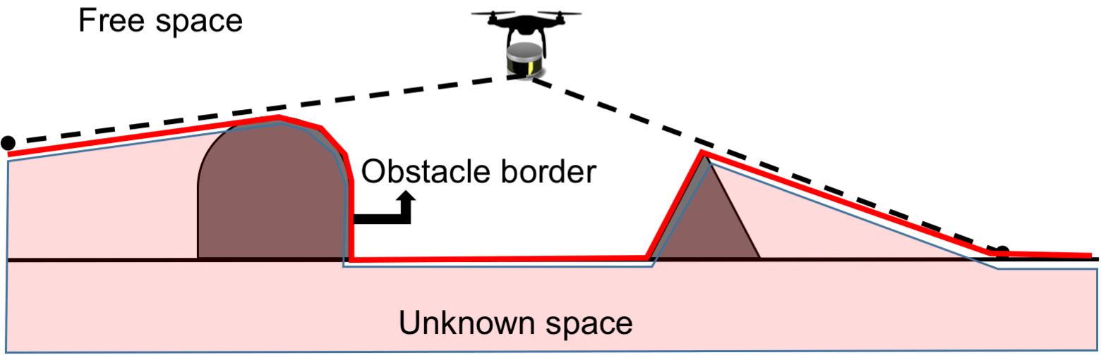
Figure 11: Diagram with our obstacle representation. Unknown voxels (red shade) are either inside of obstacles, or in zones occluded from the sensor’s field of view. The red line displays the obstacle border, which is at the interface between LiDAR hits and free space, and at the interface between unknown and free space. In this conceptual figure we assume the sensor to be onmidirectional, so the ground and obstacles below aircraft were captured as hits; however in practice the sensor has field of view limitations.

6.4 Building a Height Map

Despite keeping a full 3D map structure as the representation used for planning (Section 7), we also incrementally build a height map of the environment that is used for both the raycasting procedure when finding the actor position in world coordinates (Section 5), and for the online artistic choice selection procedure (Section 8).

The height map is a 2D array where the value of each cell corresponds to a moving average of the height of the LiDAR hits that arrive in each position. All cells are initialized with $0m$ of height, relative to the world coordinate frame, which is taken from the UAV’s takeoff position. An example height map is shown in Figure 12.

Figure 12: The left figure shows the height map accumulated over flight over a small mountain. Color scale goes from 0 ($-10$m) to 255 ($+10$m), where the zero reference of $127$ is taken at the UAV’s initial takeoff height. The right figure is the top-down view of the mountain of the same place.

7 Motion Planning

The motion planner’s objective is to calculate trajectories for the UAV to film the moving actor. Next we detail the definition of our trajectory, cost functions, the trajectory optimization algorithm, and implementation details.

7.1 UAV Trajectory Definition

Recall Section 2, where we defined $\xi_{q}(t):[0,t_{f}]\rightarrow^{3}\times SO(2)$ as the UAV trajectory and $\xi_{a}(t):[0,t_{f}]\rightarrow^{3}\times SO(2)$ as the actor trajectory, where $\xi_{q}(t)=\{x_{q}(t),y_{q}(t),z_{q}(t),\psi_{q}(t)\}$ and $\xi_{a}(t)=\{x_{a}(t),y_{a}(t),z_{a}(t),\psi_{a}(t)\}$. High-frequency measurements of the actor’s current position generate the actor’s motion forecast $\xi_{a}(t)$ in the vision module (Subsection 5.4), and it is the motion planner’s objective to output the UAV trajectory $\xi_{q}(t)$.

Since the gimbal controller can position the camera independently of the UAV’s body motion, we purposefully decouple the UAV body’s heading $\psi(t)$ from the main motion planning algorithm. We set $\psi_{q}(t)$ to always point from $\xi_{q}(t)$ towards $\xi_{a}(t)$ at all times, as seen in Equation 5.

$$\psi_{q}(t)=atan2(y_{a}(t)-y_{q}(t),x_{a}(t)-x_{q}(t))$$ (5)

This assumption significantly reduces the complexity of the planning problem by removing four degrees of freedom (three from the camera and one from the UAV’s heading), and improves filming performance because the camera can be controlled directly from image feedback, without the accumulation of errors from the raycasting module (Section 5).

Now, let $\xi_{q}(t)$ represent the UAV’s trajectory in a continuous time-parametrized form, and let $\xi_{q}$ represent the same trajectory in a finite discrete form, with total time length $t_{f}$. Let point $p_{0}$ represents the contour conditions of the beginning of the trajectory. $\xi_{q}$ contains a total of $n-1$ waypoints of the form $p_{i}$, where $i=1,...,n-1$, as shown in Equation 6.

$$\xi_{q}=\begin{bmatrix}p_{1}\\ p_{2}\\ \vdots\\ p_{n-1}\end{bmatrix}=\begin{bmatrix}p_{1x}&p_{1y}&p_{1z}\\ p_{2x}&p_{2y}&p_{2z}\\ \vdots&\vdots&\vdots\\ p_{n-1\ x}&p_{n-1\ y}&p_{n-1\ z}\\ \end{bmatrix}$$ (6)

7.2 Planner Requirements

As explained in Section 2, in a generic aerial filming framework we want trajectories which are smooth ($J_{\mathrm{smooth}}{}$), capture high quality viewpoints ($J_{\mathrm{shot}}{}$), avoid occlusions ($J_{\mathrm{occ}}{}$) and keep the UAV safe ($J_{\mathrm{obs}}{}$). Each objective can then be encoded in a separate cost function, and the motion planner’s objective is to find the trajectory that minimizes the overall cost, assumed to be a linear combination of individual cost functions, subject to the initial condition constraints. For the sake of completeness, we repeat Equation 1 below as Equation 7:

$$J\left(\xi_{q}\right) =\begin{bmatrix}1&\lambda_{1}&\lambda_{2}&\lambda_{3}\end{bmatrix}\begin{bmatrix}J_{\mathrm{smooth}}\left(\xi_{q}\right)\\ J_{\mathrm{obs}}\left(\xi_{q},\mathcal{M}\right)\\ J_{\mathrm{occ}}\left(\xi_{q},\xi_{a},\mathcal{M}\right)\\ J_{\mathrm{shot}}\left(\xi_{q},\xi_{a},\Omega_{art}\right)\end{bmatrix}$$ (7)

$$\xi_{q}^{*} =\underset{\xi_{q}}{\operatorname*{arg\,min}}\quad J\left(\xi_{q}\right),\quad\text{s.t.}\;\xi_{q}(0)=\{x_{0},y_{0},z_{0},\psi_{0}\}$$

Our choice of cost functions and planning is dictated by two main observations. First, filming requires the UAV to reason over a longer horizon than reactive approaches, usually in the order of $\sim 10$s. The UAV not only has to avoid local obstacles such as small branches or light posts, but also consider how larger obstacles such as entire trees, buildings, and terrain elevations may affect image generation. Note that the horizons are limited by how accurate the actor prediction is. Second, filming requires a high planning frequency. The actor is dynamic, constantly changing direction and velocity. The map is continuously evolving based on sensor readings. Finally, since jerkiness in trajectories have significant impact on video quality, the plans need to be smooth, free of large time discretization.

Based on these observations, we chose local trajectory optimization techniques to serve as the motion planner. Optimizations are fast and reason over a smooth continuous space of trajectories. In addition, locally optimal solutions are almost always of acceptable quality, and plans can be incrementally updated across planning cycles.

A popular optimization-based approach that addresses the aerial filming requisites is to cast the problem as an unconstrained cost optimization, and apply covariant gradient descent [Zucker et al., 2013, Ratliff et al., 2009b]. This is a quasi-Newton method, and requires that some of the objectives have analytic Hessians that are easy to invert and that are well-conditioned. With the use of first and second order information about the problem, such methods exhibit fast convergence while being stable and computationally inexpensive. The use of such quasi-Newton methods requires a set of differentiable cost functions for each objective, which we detail next.

7.3 Definition of Cost Functions

7.3.1 Smoothness

We measure smoothness as the cumulative sum of n-th order derivatives of the trajectory, following the rationale of [Ratliff et al., 2009a]. Let $D$ be a discrete difference operator. The smoothness cost is:

$$J_{\mathrm{smooth}}\left(\xi_{q}(t)\right)=\frac{1}{t_{f}}\frac{1}{2}\int_{0}^{t_{f}}\sum_{d=1}^{d_{\mathrm{max}}}\alpha_{n}(D^{d}\xi_{q}(t))^{2}dt,$$ (8)

where $\alpha_{n}$ is a weight for different orders, and $d_{\mathrm{max}}$ is the number of orders. In practice, we penalize derivatives up to the third order, setting $\alpha_{n}=1,d_{\mathrm{max}}=3$.

Appendix A.1 expands upon this cost function and reformulates it in matrix form using auxiliary matrices $A_{\mathrm{smooth}}$, $b_{\mathrm{smooth}}$, and $c_{\mathrm{smooth}}$. We state the cost, gradient and Hessian for completeness:

$$J_{\mathrm{smooth}}\left(\xi_{q}\right) =\frac{1}{2(n-1)}Tr(\xi_{q}^{T}A_{\mathrm{smooth}}\xi_{q}+2\xi_{q}^{T}b_{\mathrm{smooth}}+c_{\mathrm{smooth}})$$ (9)

$$\nabla J_{\mathrm{smooth}}\left(\xi_{q}\right) =\frac{1}{(n-1)}(A_{\mathrm{smooth}}\xi_{q}+b_{\mathrm{smooth}})$$

$$\nabla^{2}J_{\mathrm{smooth}}\left(\xi_{q}\right) =\frac{1}{(n-1)}A_{\mathrm{smooth}}$$

7.3.2 Shot quality

First, we analytically define the the artistic shot parameters. Based on cinematography literature [Arijon, 1976, Bowen and Thompson, 2013], we select a minimal set of parameters that compose most of the shots possible for single-actor, single-camera scenarios. We define $\Omega_{\mathrm{art}}$ as a set of three parameters: $\Omega_{\mathrm{art}}=\{\rho,\psi_{\mathrm{rel}},\phi_{\mathrm{rel}}\}$, where: (i) $\rho$ is the shot scale, which can be mapped to the distance between actor and camera, (ii) $\psi_{\mathrm{rel}}$ is the relative yaw angle between actor and camera, and (iii) $\phi_{\mathrm{rel}}$ is the relative tilt angle between the actor’s current height plane and the camera. Figure 13 depicts the components of $\Omega_{\mathrm{art}}$.

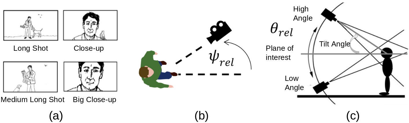
Figure 13: Shot parameters $\Omega_{\mathrm{art}}$ for shot quality cost function, adapted from [Bowen and Thompson, 2013]: a) shot scale $\rho$ corresponds to the size of the projection of the actor on the screen; b) line of action angle $\psi_{\mathrm{rel}}\in[0,2\pi]$; c) tilt angle $\theta_{\mathrm{rel}}\in[-\pi,\pi].$

Given a set $\Omega_{\mathrm{art}}$, we can now define a desired cinematography path $\xi_{shot}(t)$:

$$\xi_{shot}(t)=\xi_{a}(t)+\rho\begin{bmatrix}\cos(\psi_{a}+\psi_{rel})\sin(\theta_{rel})\\ \sin(\psi_{a}+\psi_{rel})\cos(\theta_{rel})\\ \cos(\theta_{rel})\end{bmatrix}$$ (10)

Next, we can define an analytical expression for the shot quality cost function as the distance between the current camera trajectory and the the desired cinematography path:

$$J_{\mathrm{shot}}\left(\xi_{q},\xi_{a}\right)=\frac{1}{t_{f}}\frac{1}{2}\int_{0}^{t_{f}}||\xi_{q}(t)-\xi_{shot}(\xi_{a}(t))||^{2}dt$$ (11)

Appendix A.2 expands upon this cost function and reformulates it in matrix form using auxiliary matrices $A_{\mathrm{shot}}$, $b_{\mathrm{shot}}$, and $c_{\mathrm{shot}}$. Again, we state the cost, gradient and Hessian for completeness:

$$J_{\mathrm{shot}}\left(\xi_{q},\xi_{a}\right) =\frac{1}{2(n-1)}Tr(\xi_{q}^{T}A_{\mathrm{shot}}\xi_{q}+2\xi_{q}^{T}b_{\mathrm{shot}}+c_{\mathrm{shot}})$$ (12)

$$\nabla J_{\mathrm{shot}}\left(\xi_{q}\right) =\frac{1}{(n-1)}(A_{\mathrm{shot}}\xi_{q}+b_{\mathrm{shot}})$$

$$\nabla^{2}J_{\mathrm{shot}}\left(\xi_{q}\right) =\frac{1}{(n-1)}A_{\mathrm{shot}}$$

We note that although the artistic parameters of the shot quality cost described in this work are defined for single-actor single-camera scenarios, the extension of $J_{\mathrm{shot}}$ to multi-actor scenarios is trivial. It can be achieved by defining an artistic guideline $\xi_{shot}$ using multi-actor parameters such as the angles with respect to the line of action [Bowen and Thompson, 2013], or geometric center of the targets. We detail more possible extensions of our work in Section 11.

7.3.3 Safety

Given the online map $\mathcal{G}$, we can obtain the truncated signed distance (TSDT) map $\mathcal{M}:^{3}\to$ as described in Section 6. Given a point $p$, we adopt the obstacle avoidance function from [Zucker et al., 2013]. This function linearly penalizes the intersection with obstacles, and decays quadratically with distance, up to a threshold $\epsilon_{\mathrm{obs}}$:

$$c(p)=\begin{cases}-\mathcal{M}(p)+\frac{1}{2}\epsilon_{\mathrm{obs}}&\mathcal{M}(p)<0\\ \frac{1}{2\epsilon_{\mathrm{obs}}}(\mathcal{M}(p)-\epsilon_{\mathrm{obs}})^{2}&0<\mathcal{M}(p)\leq\epsilon_{\mathrm{obs}}\\ 0&\text{otherwise}\end{cases}$$ (13)

Similarly to [Zucker et al., 2013], define a safety cost function for the entire trajectory:

$$J_{\mathrm{obs}}\left(\xi_{q},\mathcal{M}\right)=\int_{t=0}^{t_{f}}c(\xi_{q}(t))\left|\frac{d}{dt}\xi_{q}(t)\right|{}dt$$ (14)

We can differentiate $J_{\mathrm{obs}}$ with respect to a point at time $t_{i}$ to obtain the cost gradient (note that $\hat{v}=\frac{v}{|v|}$ denotes a normalized vector):

$$\nabla J_{\mathrm{obs}}\left(\xi_{q}(t_{i}),\mathcal{M}\right) =\nabla J_{\mathrm{obs}}\left(p_{i},\mathcal{M}\right)=\left|\dot{p_{i}}\right|{}\left[\;\left(I-\hat{\dot{p_{i}}}\hat{\dot{p_{i}}}^{T}\right)\nabla c(p_{i})-c(p_{i})\kappa\;\right]\;,$$ (15)

$$\text{where:}\quad\kappa=\frac{1}{\left|\dot{p_{i}}\right|{}^{2}}(I-\hat{\dot{p_{i}}}\hat{\dot{p_{i}}}^{T})\ddot{p_{i}}$$

In practice, we use discrete derivatives to calculate $\mathcal{M}$, the velocities $\dot{p_{i}}$, and accelerations $\ddot{p_{i}}$.

7.3.4 Occlusion avoidance

Even though the concept of occlusion is binary, i.e, we either have or don’t have visibility of the actor, a major contribution of our past work [Bonatti et al., 2018] was to define a differentiable cost that expresses a viewpoint’s occlusion intensity among arbitrary obstacle shapes. The fundamental idea behind this cost is that it measures along how much obstacle blockage the best possible camera viewpoints of $\xi_{q}$ would go through, assuming the camera pointed directly at the actor’s true position at all times. For illustration purposes, Figure 14 shows the concept of occlusion for motion in a 2D environment, even though our problem fully defined in 3D.

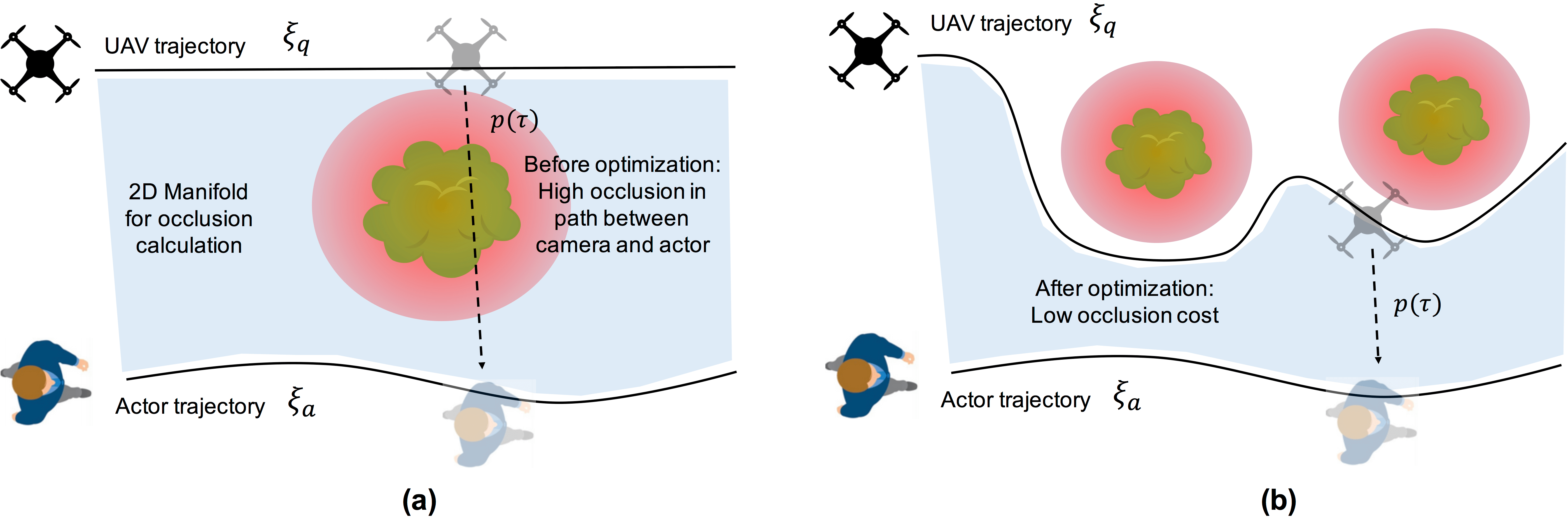
Figure 14: Occlusion cost representation. (a) For every pair of UAV-actor position, we integrate the penalization $c$ on the signed distance field over a 2D manifold. (b) After optimization, occlusion gradients pull the UAV trajectory towards regions with full visibility of the actor.

Mathematically, we define occlusion as the integral of the TSDT cost $c$ over a 2D manifold connecting both trajectories $\xi_{q}$ and $\xi_{a}$. The manifold is built by connecting each UAV-actor position pair at time $t$ using the parametrized path $p(\tau)$, where $p(\tau=0)=\xi_{q}(t)$ and $p(\tau=1)=\xi_{a}(t)$:

$$J_{\mathrm{occ}}\left(\xi_{q},\xi_{a},\mathcal{M}\right)=\int_{t=0}^{t_{f}}\left(\int_{\tau=0}^{1}\;c(p(\tau))\left|\frac{d}{d\tau}p(\tau)\right|{}d\tau\right)\,\left|\frac{d}{dt}\xi_{q}(t)\right|{}dt$$ (16)

We can derive the functional gradient with respect to a point $p_{i}$ at time $t_{i}$, resulting in:

$$\nabla J_{\mathrm{occ}}\left(\xi_{q},\xi_{a},\mathcal{M}\right)(t_{i})=\int_{\tau=0}^{1}\nabla c(p(\tau))|L||\dot{q}|\left[I-(\hat{\dot{q}}+\tau(\frac{\dot{a}}{|\dot{q}|}-\hat{\dot{q}}))\hat{\dot{q}}^{T}\right]-c(p(\tau))|\dot{q}|\left[\hat{L}^{T}+\frac{\hat{L}^{T}\dot{L}\hat{\dot{q}}{}^{T}}{|\dot{q}|}+|L|\kappa^{T}\right]d\tau,$$ (17)

where:

$$q=\xi_{q}(t_{i}),\quad a=\xi_{a}(t_{i}),\quad p(\tau)=(1-\tau)q+\tau a,,\quad L=a-q,\quad\hat{v}=\frac{v}{|v|},\quad\kappa=\frac{1}{|\dot{q}|^{2}}(I-\hat{\dot{q}}\hat{\dot{q}}^{T})\ddot{q}$$ (18)

Intuitively, the term multiplying $\nabla c(p(\tau))$ is related to variations of the signed distance gradient in space, with the rest of the term acting as a lever to deform the trajectory. The term $c(p(\tau))$ is linked to changes in path length between camera and actor.

7.4 Trajectory Optimization Algorithm

Our objective is to minimize the total cost function $J\left(\xi_{q}\right)$ (1). We do so by covariant gradient descent, using the gradient of the cost function $\nabla J(\xi_{q})$, and a analytic approximation of the Hessian $\nabla^{2}J(\xi_{q})\approx(A_{\mathrm{smooth}}+\lambda_{3}A_{\mathrm{shot}})$:

$$\xi_{q}^{+}=\xi_{q}-\frac{1}{\eta}(A_{\mathrm{smooth}}+\lambda_{1}A_{\mathrm{shot}})^{-1}\nabla J(\xi_{q})$$ (19)

In the optimization context, $\nabla^{2}J(\xi_{q})$ acts as a metric to guide the solution towards a direction of steepest descent on the functional cost. This step is repeated until convergence. We follow two conventional stopping criteria for descent algorithms based on current cost landscape curvature and relative cost decrease [Boyd and Vandenberghe, 2004], and limit the maximum number of iterations. We use the current trajectory as initialization for the next planning problem, appending a segment with the same curvature as the final points of the trajectory for the additional points until the end of the time horizon.

Note in Algorithm 2 one of the main advantages of the CHOMP algorithm [Ratliff et al., 2009a]: we only perform the Hessian matrix inversion once, outside of the main optimization loop, rendering good convergence rates [Bonatti et al., 2018]. By fine-tuning hyper-parameters such as trajectory discretion level, trajectory time horizon length, optimization convergence thresholds, and relative weights between costs, we can achieve a re-planning frequency of approximately $5$Hz considering a $10$s horizon. These are adequate parameters for safe and non-myopic operations in our environments, but lower or higher frequencies can be achieved with the same underlying algorithm depending on application-specific requirements.

1 $M_{inv}\leftarrow(A_{\mathrm{smooth}}+\lambda_{3}A_{\mathrm{shot}})^{-1}$;

2 for $i=0,1,...,i_{\mathrm{max}}$ do

3       if $(\nabla J(\xi_{q}{}_{i})^{T}M_{\mathrm{inv}}\nabla J(\xi_{q}{}_{i}))^{2}/2<\epsilon_{0}$ or $(J(\xi_{q}{}_{i})-J(\xi_{q}{}_{i-1}))<\epsilon_{1}$ then

4             return $\xi_{q}{}_{i}$;

5            

6       end if

7      $\xi_{q}{}_{i+1}=\xi_{q}{}_{i}-\frac{1}{\eta}M_{inv}\nabla J(\xi_{q}{}_{i})$;

8      

9 end for

10return $\xi_{q}{}_{i}$;

Algorithm 2 Optimize ($\xi_{q}$)

The resulting trajectory from the most recent plan is appended to the UAV’s trajectory tracker, which uses a PD controller to send velocity commands to the aircraft’s internal controller.

8 Learning Artistic Shot Selection

In this section, we introduce a novel method for online artistic shot type selection. Parameter selection which specifies the shot type can be set before deployment with a fixed set of parameters $\Omega_{\mathrm{art}}$. However, using a fixed shot type renders undesirable results during operation since the UAV does not adapt to different configurations of obstacles in the environment. Instead, here we design an algorithm for selecting adaptive shot types, depending on the context of each scene.

8.1 Deep Reinforcement Learning Problem Formulation

As introduced in Section 2, the choice of artistic parameters is a time-dependent sequential decision-making problem. Decisions taken at the current time step influence the quality of choices in future states. Figure 15 exemplifies the sequential nature of the problem.

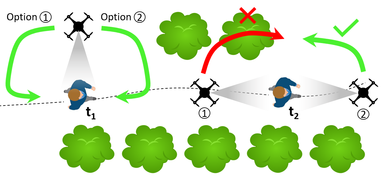
Figure 15: Example of artistic parameter selection as a sequential decision-making problem. The choice of frontal or back shots at time step $t_{1}$ influence the quality of left side shot choice at time step $t_{2}$.

We define the problem as a Contextual Markov Decision Process (C-MDP) [Krishnamurthy et al., 2016], and use an RL algorithm to find an optimal shot selection policy. Our goal is to learn a policy $\pi_{\theta}(a_{t}|c_{t})$, parametrized by $\theta$, that allows an agent to choose action $a_{t}$, given scene context $c_{t}$, to select among a discrete set of UAV artistic parameters $\Omega_{\mathrm{art}}$. Our action set is defined as four discrete values of $\Omega$ relative to left, right, back, and frontal shots. These shot types define the relative yaw angle $\phi_{\mathrm{rel}}$, which is fed into the UAV’s motion planner, as explained in Section 7.

We define state $c_{t}$ as the scene context, which is an observation drawn from the current MDP state $s_{t}$. The true state of the MDP is not directly observable because, to maintain the Markovian assumption, it encodes a diverse set of information such as: the UAV’s full state and future trajectory, the actor’s true state and future trajectory, the full history of shot types executed in past choices, a set of images that the UAV’s camera has recorded so far, ground-truth obstacle map, environmental properties such as lighting and wind conditions, etc. Therefore, our definition of context $c_{t}$ can be seen as a lower dimensional compression of $s_{t}$, given by a concatenation of following three elements:

1. Height map: a local 2.5D map containing the elevation of the obstacles near the actor;

2. Current shot type: four discrete values corresponding to the current relative position of the UAV with respect to the actor;

3. Current shot count: number of time steps the current shot type has been executed consecutively.

We assume that states evolve according to the system dynamics: $s_{t+1}\sim p(s_{t},a_{t})$. Finally, we define the artistic reward $R_{\mathrm{art}}(v_{t})$ where $v_{t}(s_{t},a_{t})=\{I_{1},I_{2},...,I_{k}\}$ is the video taken after the UAV executed action $a_{t}$ at state $s_{t}$. Our objective is to find the parameters of the optimal policy, which maximizes the expected cumulative reward:

$$\theta^{*}=\underset{\theta}{\operatorname*{arg\,max}}\quad\mathbb{E}\left[\sum_{t=1}^{T}R_{\mathrm{art}}(v_{t})\right],$$ (20)

where the expectation accounts for all randomness in the model and the policy. A major challenge for solving Equation 20 is the difficulty of explicitly modeling the state transition function $p(s_{t},a_{t})$. This function is dependent on variables such as the quadrotor and actor dynamics, the obstacle set, the motion planner’s implicit behavior, the quadrotor and camera gimbal controllers, and the disturbances in the environment. In practice, we cannot derive an explicit model for the transition probabilities of the MDP. Therefore, we use a model-free method for the RL problem, using an action-value function $Q(c_{t},a_{t})$ to compute the artistic value of taking action $a_{t}$ given the current context $c_{t}$:

$$Q(c_{t},a_{t})=\sum_{t^{\prime}=t}^{T}\mathbb{E}_{\pi_{\theta}}\left[R_{\mathrm{art}}(v(c_{t^{\prime}},a_{t^{\prime}}))|c_{t},a_{t}\right]$$ (21)

The large size and complexity of the state space for our application motivates us to use a deep neural network with parameters $\theta$ to approximate $Q$: $Q(c_{t},a_{t})\approx f(c_{t},a_{t},\theta)$ [Sutton and Barto, 1998, Mnih et al., 2013].

8.2 Reward Definition

Now we define the artistic reward function $R\textsubscript{art}$. At a high level, we define the following basic desired aesthetical criteria for an incoming shot sequence:

• Keep the actor within camera view for as much time as possible;

• Maintain the tilt viewing angle $\theta\textsubscript{t}$ within certain bounds; neither too low nor too high above the actor;

• Vary the relative yaw viewing angle over time, in order to show different sides of the actor and backgrounds. Constant changes keep the video clip interesting. However, too frequent changes don’t leave the viewer enough time to get a good overview of the scene;

• Keep the drone safe, since collisions at a minimum destabilize the UAV, and usually cause complete loss of actor visibility due to a crash.

While these basic criteria represent essential aesthetical rules, they cannot account for all possible aesthetical requirements. The evaluation of a movie clip can be highly subjective, and depend on the context of the scene and background of the evaluator. Therefore, in this work we compare two different approaches for obtaining numerical reward values. In the first approach we hand-craft an arithmetical reward function $R_{\mathrm{art}}$, which follows the basic aesthetics requirements outlined above. In addition, we explore an alternative approach for obtaining $R_{\mathrm{art}}$ directly from human supervision. Next, we describe both methods.

Hand-crafted reward:

The reward calculation from each control time step involves the analysis and evaluation of each frame of the video clip. Since our system operates with steps that last $6$s, the reward value depends on the evaluation of $180$ frames, given that images arrive at $30$Hz. We define $R_{\mathrm{frame}}$ as the sub-reward relative to each frame, and compute it using the following metrics:

Shot angle: $R_{\mathrm{frame}}^{\mathrm{shot}}$ considers the current UAV tilt angle $\theta_{\mathrm{rel}}$ in comparison with an optimal value $\theta_{\mathrm{opt}}=15^{\circ}$ and an accepted tolerance $\theta_{\mathrm{tol}}=\pm 10^{\circ}$ around it. The shot angle sub-reward decays linearly and symmetrically between $1.0$ and $0.0$ from $\theta_{\mathrm{opt}}$ to the tolerance bounds. Out of the bounds, we assign a negative penalty of $R_{\mathrm{frame}}^{\mathrm{shot}}=-0.5$.

Actor’s presence ratio: considers the screen space occupied by the actor’s body. We set two bounds $pr_{\mathrm{min}}=0.05$ and $pr_{\mathrm{max}}=0.10$ based on a desired long-shot scale, actor size of $1.8$m, and the camera’s intrinsic matrix. If the presence ratio lies within the bounds, we set the value of $R_{\mathrm{frame}}=R_{\mathrm{frame}}^{\mathrm{shot}}$. Otherwise, this parameter indicates that the current frame contains very low aesthetics value, with the actor practically out of the screen or occupying an exorbitant proportion of it. In that case, we set a punishment $R_{\mathrm{frame}}=-0.5$.

We average the resulting $R_{\mathrm{frame}}$ over all frames present in one control step to obtain an intermediate reward $R_{\mathrm{step}}=\frac{1}{N}\sum_{i=1}^{N}R_{\mathrm{frame,\ i}}$. Next, we consider the interaction between consecutive control steps to discount $R_{\mathrm{step}}$ using a third metric: shot type duration.

Shot type duration: considers the duration of the current shot type, given by the count of steps $c$ in which the same action was selected sequentially. We use the heuristic that the ideal shot type has a length $12$s, or $c_{\mathrm{opt}}=2$ time steps, and define a variable discount parameter $\alpha_{c}$, as seen in Fig. 16. High repetition counts are penalized quadratically to maintain the viewers interested in the video clip.

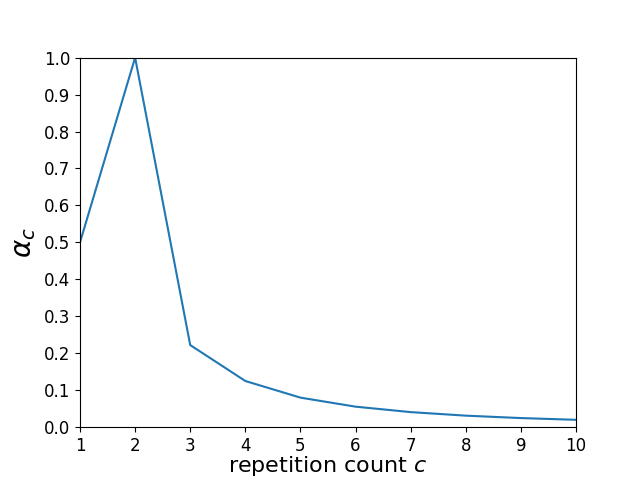
Figure 16: Values of the variable discount parameter $\alpha_{c}$ over shot repetition counts $c$.

Eq. (22) shows how we obtain the final artistic reward $R_{\mathrm{art}}$ for the current movie clip. If $R_{\mathrm{step}}$ is positive, $\alpha_{c}$ serves as a discount factor, with the aim of guiding the learner towards the optimal shot repetition count. In the case of negative $R_{\mathrm{step}}$, we multiply the reward by the inverse $\alpha_{c}$, with the objective of accentuating the penalization, and to incentivize the policy to quickly recover from executing bad shot types repetitively.

$$R_{\mathrm{art}}=\begin{cases}R_{\mathrm{step}}\cdot\alpha_{c},&\text{if }R_{\mathrm{step}}\geq 0\\ \frac{R_{\mathrm{step}}}{\alpha_{c}},&\text{otherwise.}\end{cases}$$ (22)

In the eventual case of a UAV collision during the control step we override the reward calculation procedure to only output a negative reward of $R_{\mathrm{art}}=-1.0$.

Human supervision reward:

We also explore a reward scheme for video segments based solely on human evaluation. We create an interface (Fig. 17) in which the user gives an aesthetics score between 1 (worst) and 5 (best) to the video generated by the previous shot selection action. The score is then linearly mapped to a reward $R_{\mathrm{art}}$ between $-0.5$ and $1.0$ to update the shot selection policy in the RL algorithm. In the case of a crash during the control step, we override the user’s feedback with a penalization of $R_{\mathrm{art}}=-1.0$.

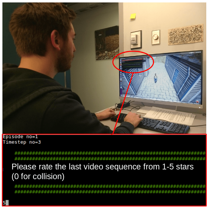
Figure 17: Evaluators rate video clips during the training procedure using an interface on the screen.

8.3 Implementation Details

Our DQN architecture is composed of different linear layers which combine the state inputs, as seen in Figure 18. We use ReLU functions after each layer except for the last, and use the Adam optimizer [Kingma and Ba, 2014] with Huber loss [Huber et al., 1964] for creating the gradients. We use an experience replay (ER) buffer for training the network, such as the one described by [Mnih et al., 2015].

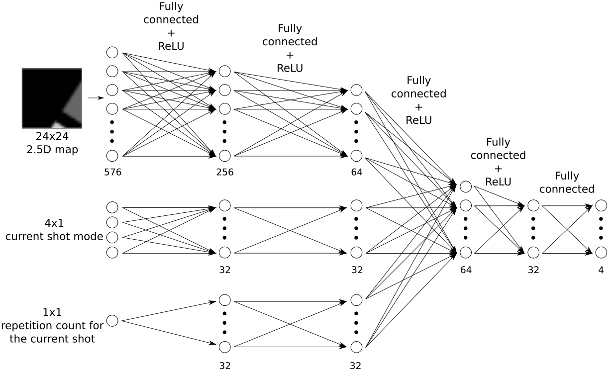
Figure 18: DQN architecture consisting of fully connected layers. Each portion of state is first fed to separate mini-networks of two layers. Then, the outputs of these are combined in three consecutive layers whose output is the Q values.

9 Experimental Results

In this section we detail integrated experimental results, followed by detailed results on each subsystem.

9.1 Integrated System Results

We conducted a series of field trials to evaluate our integrated system in real-life conditions. We used a large open facility named Gascola in Penn Hills, PA, located about $20$ min east of Pittsburgh, PA. The facility has a diverse set of obstacle types and terrain types such as several off-road trails, large mounds of dirt, trees, and uneven terrain. Figure 19 depicts the test site and shows the different areas where the UAV flew during experiments. We summarize the test’s objectives and results in Table 3, and indicate which results explain our initial hypotheses from Subsection 4.1.

Table 3: Objectives and results for integrated experiments.

Objectives	Results
Stay safe among unstructured obstacles sensed online (addresses Hyp.1)	Avoided all obstacles successfully, including trees, dirt mound, slopes, posts. See Figs. 20-21.
Avoid occlusions among any obstacle shape (addresses Hyp.1)	Planner maintained actor visibility. See Fig. 20. More results in Subsec 9.3.
Process data fully onboard (addresses Hyp.1)	Data processed solely on onboard computer. Table 4 and Fig. 22 show system statistics.
Operate with different types of actors at different speeds (addresses Hyps.2-3)	Person, car, bikes shot at high-speed chases. See Figs. 20-23.
Execute different shot types (addresses Hyp.3)	Successful recording of back, right, front, circling shots (Fig. 20). Smooth shot transitions (Fig. 23).
Automatically select artistically meaningful shot types (addresses Hyp.3)	Policy adapted to current context to produce a visually aesthetic video. Fig. 23.

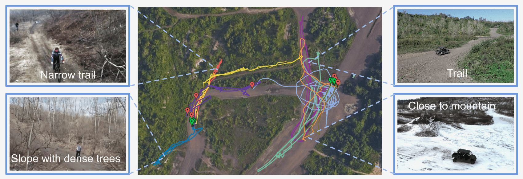
Figure 19: Testing facility. The middle figure shows a top-down satellite view of testing terrain, overlayed with UAV positions from different trials. We accumulated over $2$h of flight time, and a total distance of almost $6$km. The side figures show the diverse types of terrains in our experiments. The figures also depict different actors and different seasons.

Figure 20 summarizes our experiments conducted with fixed shot types. We employ a variety of shot types and actors, while operating in a wide range of unstructured environments such as open fields, in proximity to a large mound of dirt, on narrow trails between trees and on slopes. In addition, Figure 21 provides a detailed time lapse of how the planner’s trajectory output evolves during flight through a narrow trail between trees.

Figure 23 shows experiments where we employed the online automatic artistic selection module. In-depth results of this module are described in Subsection 9.4.

We also summarize our integrated system’s runtime performance statistics in Table 4, and discuss details of the online mapping performance in Figure 22. Videos of the system in action can be found attached with the submission, or online at https://youtu.be/ookhHnqmlaU.

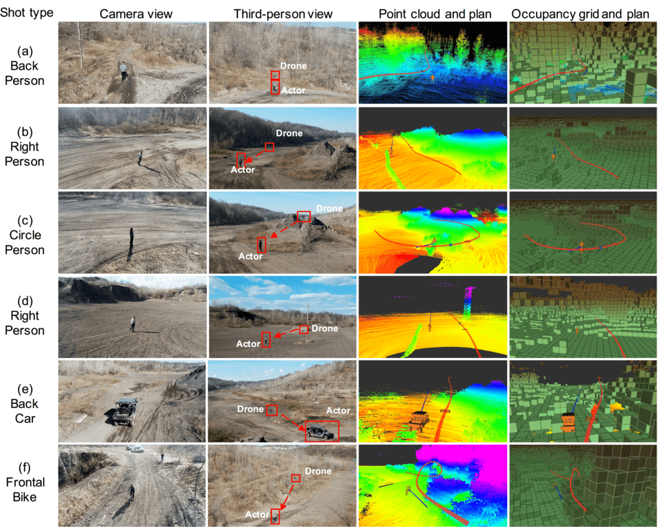
Figure 20: Field results with different fixed shot types in multiple environment types, following different actor types. The UAV trajectory (red) tracks the actor’s forecasted motion (blue), and stays safe while avoiding occlusions from obstacles. We display accumulated point clouds of LiDAR hits and the occupancy grid: a) Back shot following runner in narrow tree trail; b) Right side shot following a runner close to dirt mound; c) Circular shot on person close to dirt mound; d) Right side shot below the 3D structure of an electric wire. Note that LiDAR registration is noisy close to the pole in row due to large electromagnetic interference with the UAV’s compass; e) Right side shot following car close to dirt mound; f) Frontal shot on biker going downhill on a trail with tall trees.

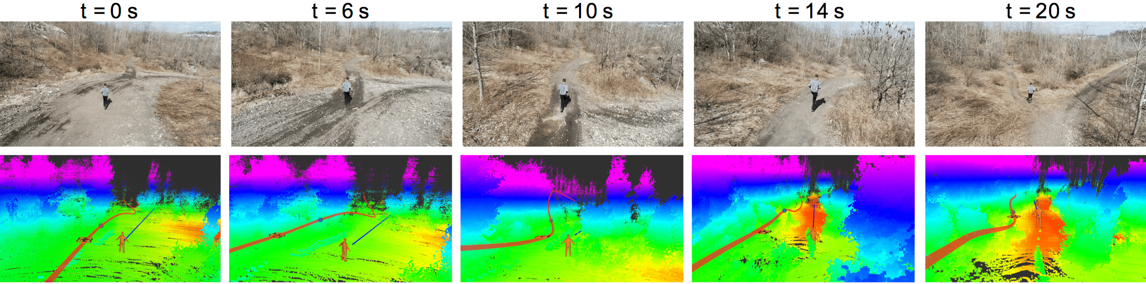
Figure 21: Detailed time lapse of back shot following a runner in a narrow trail with trees. As the UAV approaches the trees at $t=6$s, the trajectory bends to keep the vehicle safe, maintain target visibility, and follow the terrain’s downwards inclination.

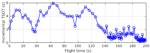
Figure 22: Incremental distance transform computation time over flight time. The first operations take significantly more time because of our map initialization scheme where all cells are initially considered as unknown instead of free, causing the first laser scans to update a significantly larger number of voxels than later scans. During calculation the planner is not blocked: it can still access TSDT values from the latest version of $\mathcal{M}$.

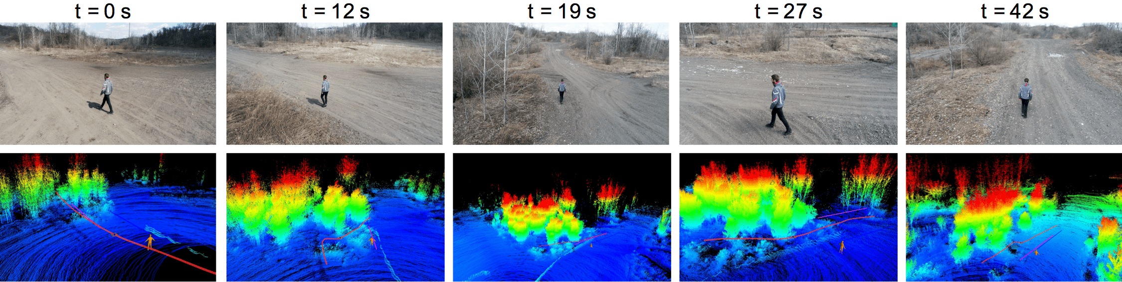
Figure 23: Field test results using the online artistic shot selection module. UAV trajectory is shown in red, actor motion forecast in blue, and desired shot reference in pink. The UAV initially does a left side shot at $t=0$s in the open field, but as a line of trees appear, it switches to a back shot at $t=12$s. When an opening appears among the tree lines, the UAV selects a left side shot again at $t=27$s, and when the clearance ends, the module selects a back shot again.

Table 4: System statistics recorded during flight time on onboard computer.

0.2cmSystem	1.0cmModule	2.0cmCPU
	2.0cmRAM (MB)	2.0cmRuntime (ms)	2.0cmTarget freq. (Hz)
	Detection	57	2160	145
Vision	Tracking	24	25	14.4	15
	Heading	24	1768	13.9
	KF	8	80	0.207
	Grid	22	48	36.8
Mapping	TSDF	91	810	100-6000	10
	LiDAR	24	9	100
Planning	Planner	98	789	198	5
Controls	DJI SDK	89	40	NA	50
Shot selection	DQN	4	1371	10.0	0.16

From the field experiments, we verify that our system achieved all system-level objectives in terms of safely and robustly executing a diverse set of aerial shots with different actors and environments. Our data also confirms the questions raised to validate our hypotheses: onboard sensors and computing power sufficed to provide smooth plans, producing artistically appealing images.

Next we present detailed results on the individual sub-systems of the aircraft.

9.2 Visual Actor Localization and Heading Estimation

Here we detail dataset collection, training and testing of the different subcomponents of the vision module. We summarize the vision-specific test’s objectives and results in Table 5.

Table 5: Objectives and results for vision-specific experiments.

Objectives	Results
Compare object detection network architectures	Faster-RCNN showed significantly better performance than SSD architecture (Fig. 24).
Compare supervised and semi-supervised methods for heading estimation	Semi-supervised method has smoother output and higher accuracy(Table 7 and Fig. 25 )
Analyze the amount of labeled data needed for semi-supervised training	Loss increased by less than $\sim 8\%$ when we trained the model with $1/10$ of labeled data (Fig. 26)
Validate integrated 3D pose estimator using image projections	Error of less than $1.7$m in estimated actor path length over a $40$m long ground-truth actor trajectory (Fig. 27).

9.2.1 Object detection network

Dataset collection. We trained the network on the COCO dataset [Lin et al., 2014], and fine-tuned it with a custom aerial filming dataset. To test, we manually labeled 120 images collected from our aerial filming experiments, with bounding box over people and cars.

Training procedure: We trained and compared two architectures: one based on Faster-RCNN, another on SSD. As mentioned in Section 5, we simplify feature extraction with MobileNet-based structure to improve efficiency. First we train both structures on the COCO dataset. While the testing performance is good on the COCO testing dataset, the performance shows a significant drop, when tested on our aerial filming data. The network has a low recall rate (lower than 33%) due to big angle of view, distant target, and motion blur. To address the generalization problem, we augmented the training data by adding blur, resizing and cropping images, and modifying colors. After training on a mixture of COCO dataset [Lin et al., 2014] and our own custom dataset as described in Section 5, Figure 24 show the recall-precision curve of the two networks when tested on our filming testing data. The SSD-based network has difficulties detecting small objects, an important need for aerial filming. Therefore, we use Faster-RCNN-based network in our experiments and set the detection threshold to precision=0.9, as shown with the green arrow in Figure 24.

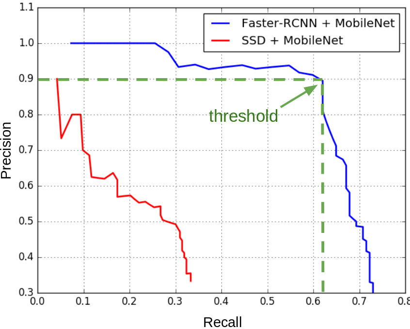
Figure 24: Precision recall curve for object detection. The results are tested on the filming testing data, which contains many challenging cases.

9.2.2 Heading direction estimation (HDE) network

Dataset collection:

We collected a large number of image sequences from various sources. For the person HDE, we used two surveillance datasets: VIRAT [Oh et al., 2011] and DukeMCMT [Ristani et al., 2016], and one action classification dataset: UCF101 [Soomro et al., 2012]. We manually labeled 453 images in the UCF101 dataset as ground-truth HDE. As for the surveillance datasets, we adopted a semi-automatic labeling approach where we first detected the actor in every frame, then computed the ground-truth heading direction based on the derivative of the subject’s position over a sequence of consecutive time frames. For the car HDE we used two surveillance datasets, VIRAT and Ko-PER [Strigel et al., 2014], in addition to one driving dataset, PKU-POSS [Wang et al., 2016]. Table 6 summarizes our data.

Table 6: Datasets used in HDE study. *MT denotes labeling by motion tracking, HL denotes hand labels.

Dataset	Target	GT	No. Seqs	No. Imgs
VIRAT	Car/Person	MT*	650	69680
UCF101	Person	HL(453)*	940	118027
DukeMCMT	Person	MT*	4336	274313
Ko-PER	Car	$\checkmark$	12	18277
PKU-POSS	Car	$\checkmark$	-	28973

Training the network:

We first train the HDE network using only labeled data from the datasets shown in Table 6. Rows 1-3 of Table 7 display the results. Then, we fine-tune the model with unlabeled data to improve generalization.

We collected 50 videos, each contains approximately 500 sequential images. For each video, we manually labeled 6 images. The HDE model is finetuned with both labeled loss and continuity loss, same as the training process on the open accessible datasets. We qualitatively and quantitatively show the results of HDE using semi-supervised finetuning in Figure 25 and Table 7. The experiment verifies our model could generalize well to our drone filming task, with a average angle error of $0.359$ rad. Compared to the pure supervised learning, utilizing unlabeled data improves generalization and results in more robust and stable performance.

Figure 25: Three models are tested on the sequential data. Two testing sequences are shown in this figure. The top row of each testing sequence shows the results that directly employ the model trained on other open accessible datasets to the aerial filming task. It generalizes poorly due to the distribution difference. The middle row and bottom row show the results after finetuning the model on the filming data with and without continuity loss, respectively. The model using continuity loss for finetuning (bottom row) outputs more accurate and smooth results.

Baseline comparisons: We compare our HDE approach against two baselines. The first baseline Vanilla-CNN is a simple CNN inspired by [Choi et al., 2016]. The second baseline CNN-GRU implicitly learns temporal continuity using a GRU network inspired by [Liu et al., 2017]. One drawback for this model is that although it models the temporal continuity implicitly, it needs large number of labeled sequential data for training, which is very expensive to obtain.

We employ three metrics for quantitative evaluation: 1) Mean square error (MSE) between the output $(\cos\theta,\sin\theta)$ and the ground truth $(\hat{\cos\theta},\hat{\sin\theta})$. 2) Angular difference (AngleDiff) between the output and the ground truth. 3) Accuracy obtained by counting the percentage of correct outputs, which satisfies AngleDiff$<\pi/8$. We use the third metric, which allows small error, to alleviate the ambiguity in labeling human heading direction.

Vanilla-CNN [Choi et al., 2016] and CNN-GRU [Liu et al., 2017] baselines trained on open datasets don’t transfer well to drone filming dataset with accuracy below 30%. Our SSL based model trained on open datasets achieves 48.7% accuracy. By finetuning on labelled samples of drone filming, we improve this to 68.1%. Best performance is achieved by finetuning on labelled and unlabeled sequences of the drone filming data with accuracy of 72.2% (Table 7).

Table 7: Semi-Supervised Finetuning results

Method	MSE loss	AngleDiff (rad)	Accuracy (%)
Vanilla-CNN w/o finetune	0.53	1.12	26.67
CNN-GRU w/o finetune	0.5	1.05	29.33
SSL w/o finetune	0.245	0.649	48.7
SL w/ finetune	0.146	0.370	68.1
SSL w/ finetune	0.113	0.359	72.2

Reduction in required labeled data using semi-supervised learning: Following Section 5, we show how semi-supervised learning can significantly decrease the number of labeled data required for the HDE task.

In this experiment, we train the HDE network on the DukeMCMT dataset, which consists of 274k labeled images from 8 different surveillance cameras. We use the data from 7 cameras for training, and one for testing (about 50k). Figure 26 compares result from the proposed semi-supervised method with a supervised method using different number of labeled data. We verify that by utilizing unsupervised loss, the model generalizes better to the validation data than the one with purely supervised loss.

As mentioned, in practice, we only use 50 unlabeled image sequences, each containing approximately 500 sequential images, and manually labeled 300 of those images. We achieve comparable performance with purely supervised learning methods, which require more labeled data.

Figure 26: The top row shows training and validation loss for supervised learning using different number of labeled data. The validation performance drops from 0.13 to 0.22, when decreasing the number of labeled data from 100% to 1%. The bottom row shows results with semi-supervised learning. The validation losses are 0.13, 0.14 and 0.17 respectively for 100%, 10% and 1% labeled data.

9.2.3 3D pose estimation

Based on the detected bounding box and the actor’s heading direction in 2D image space, we use ray-casting method to calculate the 3D pose of the actor, given the online occupancy map and the camera pose. We assume the actor is in a upward pose, in which case the pose is simplified as $(x,y,z,\psi_{a}^{w})$, which represents the position and orientation in the world frame.

We validate the precision of our 3D pose estimation in two field experiments where the drone hovers and visually tracks the actor. First, the actor walks between two points along a straight line, and we compare the estimated and ground truth path lengths. Second, the actor walks in a circle at the center of a football field, and we compute the errors in estimated position and heading direction. Figure 27 shows our estimation error is less than 5.7%.

Figure 27: Pose and heading estimation results. a) Actor walks on a straight line from points A-B-A. Ground-truth trajectory length is 40.6m, while the estimated motion length is 42.3m. b) The actor walks along a circle. Ground-truth diameter is 18.3m, while the estimated diameter from ray casting is 18.7m. Heading estimation appears tangential to the ground circle.

9.3 Planner Evaluation

Next we present detailed results on different aspects of the UAV’s motion planner. Table 8 summarizes the experiments’ objectives and results.

Table 8: Objectives and results for detailed motion planner experiments.

Objectives	Results
Performance comparison between online vs. ground-truth map	Similar path quality, with increase in planning time. See Fig. 28 and Table 9.
Performance comparison between noisy actor forecast vs. ground-truth actor positioning	Similar path quality: smoothness cost handles noisy inputs. See Fig. 29.
Confirm ability to operate in full 3D environments	Can fly under 3D obstacles, not only height maps. See Fig. 20-d.
Performance comparison between different planning time horizons	Longer horizons significantly improve path quality. See Fig. 30 and Table 10.
Test impact of occlusion cost function on actor visibility	Occlusion cost significantly improves path quality. See Fig. 32, Fig. 31, and Table 11.

Ground-truth obstacle map vs. online map: We compare average planning costs between results from a real-life test where the planner operated while mapping the environment in real time with planning results with the same actor trajectory but with full knowledge of the map beforehand. Results are averaged over 140 s of flight and approximately 700 planning problems. Table 9 shows a small increase in average planning costs with online map, and Fig 28 shows that qualitatively both trajectories differ minimally. The planning time, however, doubles in the online mapping case due to mainly two factors: extra load on CPU from other system modules, and delays introduced by accessing the map that is constantly being updated. Nevertheless, computation time is low enough such that the planning module can still operate at the target frequency of $5$ Hz.

Figure 28: Performance comparisons between planning with full knowledge of the map (yellow) versus with online mapping (red), displayed over ground truth map grid. Online map trajectory is less smooth due to imperfect LiDAR registration and new obstacle discoveries as flight progresses.

Table 9: Performance comparison between ground-truth and online map.

4cmPlanning condition	4cmAvg. plan time(ms)	2cmAvg. cost	3cmMedian cost
Ground-truth map	32.1	0.1022	0.0603
Online map	69.0	0.1102	0.0825

Ground-truth actor pose versus noisy estimate: We compare the performance between simulated flights where the planner has full knowledge of the actor’s position versus artificially noisy estimates with $1$m amplitude of random noise. The qualitative comparison with the actor’s ground-truth trajectory shows close proximity of both final trajectories, as seen in Fig 29.

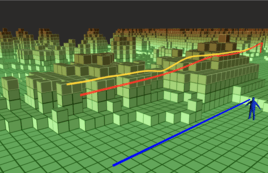
Figure 29: Performance comparison between planning with perfect ground truth of actor’s location (red) versus noisy actor estimate with artificial noise of 1m amplitude (yellow). The planner is able to handle noisy actor localization well due to smoothness cost terms, with final trajectory similar to ground-truth case.

Operation on unstructured 3D map: As seen in Figure 20d, our current system is able to map and avoid unstructured obstacles in 3D environments such as wires and poles. This capability is a significant improvement over previous work that only deals with ellipsoidal obstacle representations [Nägeli et al., 2017, Joubert et al., 2016, Huang et al., 2018a], or a height map assumption [Bonatti et al., 2018].

Advantage of longer planning horizons: We evaluate the overall system behavior when using different planning time horizons between $1$ and $20$ seconds, as seen in Table 10. Short horizons reason myopically about the environment, and cannot render robust and safe behavior in complex scenes, thus increasing the normalized cost per time length of the resulting trajectory. Figure 30 displays the qualitative difference between trajectories, keeping all variables except planning horizon constant.

Table 10: Performance of motion planner with varying planning time horizons for the environment shown in Fig 30. Longer planning horizons allow better reasoning for safety and occlusion avoidance, lowering the normalized planning cost. However, longer horizons naturally increase planning computing time.

Planning horizon length [s]:	1.0	5.0	10.0	20.0
Normalized trajectory cost [$J$/$t_{f}$]	0.0334	0.0041	0.0028	0.0016
Computing time [ms]	0.0117	0.0131	0.0214	0.0343

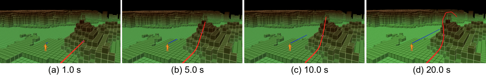
Figure 30: Planner behavior with different time horizons of $1$ (a), $5$ (b), $10$ (c), and $20$ (d) seconds for same actor trajectory and environment. The shortest time horizon of $1$s is not sufficient for the planner to find a trajectory that avoids the mound, and the vehicle gets stuck in a bad local minimum of solutions. Longer horizons let the UAV plan more intelligent trajectories, reasoning about obstacle shapes long before the UAV reaches those positions.

Qualitative role of the occlusion cost function: For this experiment, unlike the tests with visual actor localization, we detect the actor using a ground-truth GPS tag. We set up the motion planner to calculate the UAV paths with and without the occlusion cost function, keeping all other scenario variables equal. As seen in Figure 31, our proposed occlusion cost significantly improves the aesthetics of the resulting image, keeping the actor visibility. In addition to aesthetics, maintaining actor visibility is a vital feature of our architecture, allowing vision-based actor localization.

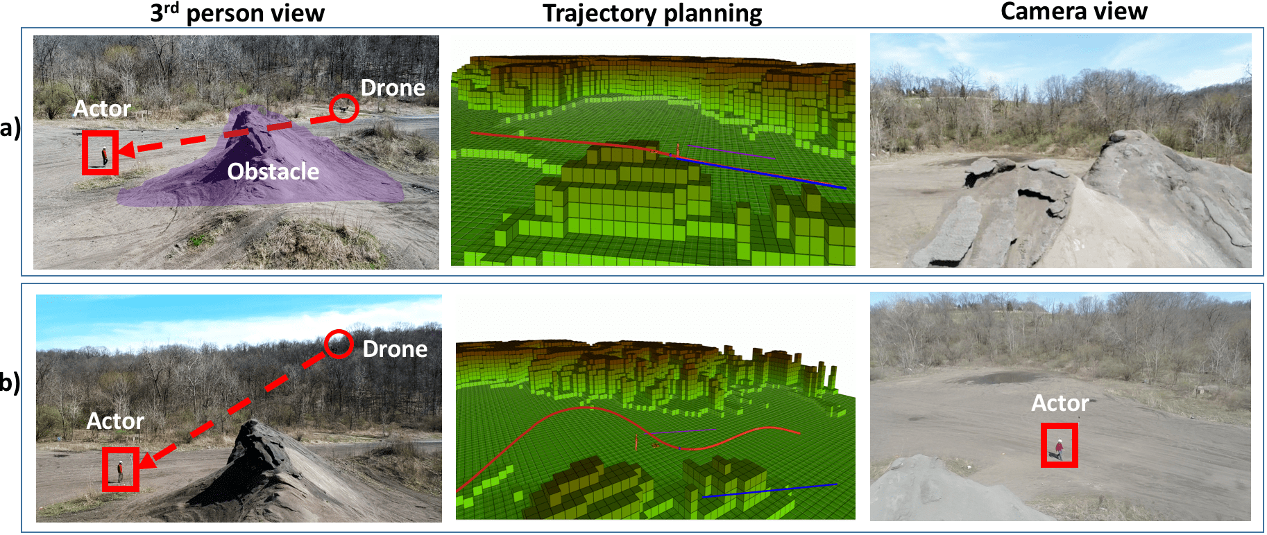
Figure 31: Comparison of planning a) without and b) with occlusion cost function in a special setup where actor positioning comes from a GPS tag. The occlusion cost function significantly improves the quality of the camera image in comparison with pure obstacle avoidance, for same shot type.

Quantitative role of the occlusion cost function: We evaluate our planning algorithm on environments with increasing levels of randomized clutter, as seen in Figure 32. Table 11 summarizes the planner performance in different environments in terms of actor visibility and the average distance to the artistically desired trajectory. By using the occlusion cost function, we improve actor visibility by over 10% in comparison with pure obstacle avoidance in environments with 40 random spheres; however, the trade-off is an increase in the average distance to the desired artistic trajectory.

Table 11: Evaluation of motion planner performance in the randomized environment from Fig 32. Statistics computed using $100$ random configurations for each environment complexity level.

		Num. of spheres in environment
Success metric	Cost functions	1	20	40
Actor visibility	$J_{\mathrm{occ}}+J_{\mathrm{obs}}$	$99.4\pm 2.2\%$	$94.2\pm 7.3\%$	$86.9\pm 9.3\%$
along trajectory	$J_{\mathrm{obs}}$	$98.8\pm 3.0\%$	$87.1\pm 8.5\%$	$75.3\pm 11.8\%$
Avg. dist. to $\xi_{\mathrm{shot}}$,	$J_{\mathrm{occ}}+J_{\mathrm{obs}}$	$0.4\pm 0.4$	$6.2\pm 11.2$	$10.7\pm 13.2$
in m	$J_{\mathrm{obs}}$	$0.05\pm 0.1$	$0.3\pm 0.2$	$0.5\pm 0.3$

Figure 32: Randomized environment with obstacles to evaluate planner robustness. UAV trajectory initialization shown in blue, actor trajectory in purple, and planner iterations vary from red to green (final solution). a) Solution including occlusion cost function, and b) Pure obstacle avoidance.

These detailed results allow us to draw insights into the planner performance under different conditions: it can operate smoothly, in full 3D maps, even under noise of real-time environment mapping and noisy actor inputs. We can also verify the importance of the efficient optimization algorithm for planning: by allowing longer time horizons, we can generate significantly higher quality plans. Finally, we demonstrate the essential role of our occlusion cost, which is defined for arbitrary obstacle shapes in the environment, in maintaining actor visibility.

9.4 Artistic Shot Selection

Next we present detailed results on training and testing the artistic shot selection module, as well as experiments that provide insights to understand which artistic concepts this subsystem is learning. Table 12 summarizes our test objectives and results.

We trained our agent exclusively in simulation, using the Microsoft AirSim release (see Section 4.4). We organize our environments in three categories:

• BlockWorld: It is generated from a height map, and the actor walks on a path with alternating blocks on the left and right sides. Blocks have varying heights and lengths (Figure 33a).

• BigMap: It is generated from a height map, and significantly more complex. It is separated into three zones: one that resembles the BlockWorld environment, a second zone with alternating pillars, and third zone with different shapes of mound-like structures (Figure 33b).

• Neighborhood: Unlike the two previous height maps, this environment is a photo-realistic rendering of a suburban residential area. The actor walks among structures like streets, houses, bushes, trees, and cars (Figure 33c).

Table 12: Objectives and results for artistic shot selection.

Objectives	Results
Compare policy generalizability to different environments	Learned policies generalized well to new unseen environments. Table 13 compares performances.
Analyze role of specific environment context in policy behavior	Policy learned to actively avoid potential occlusions and switch often to keep video interesting (Figs. 34-35)
Evaluate policies against baselines using real human aesthetics in user study	Our policy outperformed constant shot types or random actions (Table 14 and Fig. 36)
Transfer policy learned in simulation to real-life environments	We deployed the policy in additional field experiments (Fig. 37).

Figure 33: Rendering and height maps of AirSim environments with training routes. a) BlockWorld 1 (red), BlockWorld 2 (blue) b) Bigmap (yellow) c) Neighborhood 1 (orange), Neighborhood 2 (purple).

9.4.1 Learning an artistic policy

Hand-crafted reward: Using the hand-crafted reward definition from Section 8, we train a total of six policies in different environments. For all policies except Neighborhood 1 roam, the actor walks along a pre-defined path. We define each episode as a concatenation of 5 consecutive time steps, each with a duration of $6$ seconds, and we train each policy between 300 to 2000 episodes, depending on the complexity of the environment:

• BlockWorld 1 and 2: Trained in different randomized BlockWorld environments, BW1 and BW2, for 300 episodes.

• BigMap: Trained in a randomized BigMap environment, BM, for 1500 episodes.

• Neighborhood 1 and 2: Trained in different sections of the Neighborhood environment, NH1 and NH2. Trained for 500 episodes.

• Neighborhood roam: Trained in the entirety of the Neighborhood environment NH, with actor walking in random motion, for 2000 episodes.

We test all policies in all environments to evaluate generalizability. Table 13 summarizes the quantitative results. As expected, all policies perform better than random choice, and we achieve highest testing rewards in the same environments the policies were trained in. We also verify that the best generalization performance occurs when policies are trained and tested on the same environment category. It is interesting to note that policies trained on the Neighborhood environments tested on BigMap perform significantly better than those trained on BlockWorld, likely due to the simple geometry of the BlockWorld obstacles.

Table 13: Average reward per time step. As expected, policies have the highest rewards when trained and tested on the same environment (bold diagonal). The second-best policy for each environment is underlined and italicized.

	BW1	BW2	BM	NH1	NH2
BlockWorld 1	0.3444	0.3581	0.3635	0.3622	0.2985
BlockWorld 2	0.3316	0.3718	0.3918	0.4147	0.3673
BigMap	0.2178	0.2506	0.5052	0.5142	0.5760
Neighborhood 1	0.1822	0.1916	0.4311	0.5398	0.5882
Neighborhood 2	0.0813	0.1228	0.4488	0.4988	0.5897
Neighborhood 1 roam	0.1748	0.1779	0.4394	0.5221	0.5546
Random choice	-0.0061	0.0616	0.1944	0.2417	0.2047

Figures 34 and 36 show examples of trajectories generated with trained policies. In addition, Figure 35 shows a heatmap with different actions, providing insights into the learned policy’s behavior. Qualitatively, we observe that the learned behavior matches the intended goals:

• Keeps the actor in view by avoiding drastic shot mode switches between opposite positions such as left and right or front and back, which often cause visual loss of the actor;

• Switches shot types regularly to keep the viewer’s interest;

• Avoids flying above high obstacles to keep the shot angle within desirable limits;

• Avoids high obstacles to maintain aircraft safety.

Human-generated rewards: Using the interface described in Section 8, we use human aesthetics evaluations as rewards to train two new policies in the BlockWorld and Neighborhood environments for 300 and 500 episodes respectively. Comparisons between both reward schemes are presented next.

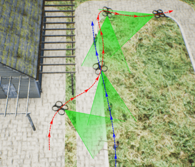
Figure 34: Time lapse of drone trajectory during filming in photo-realistic environment. Since the left hand side is occupied, the drone switches from left to front and then right shot.

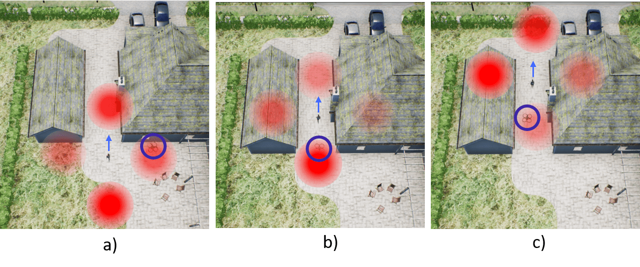
Figure 35: Visualization of the Q-values of the DQN during testing corresponding to the 4 shot types. The more opaque a circle is, the higher is the action’s Q-value. The drone position before each decision is indicated by a blue ring around the drone. The drone starts on the right side of the actor and switches to back shot mode to traverse a narrow passage (a) where it stays in the actor’s back for one time step (b). Finally it decides to switch to a left side shot once the obstacles are passed (c).

9.4.2 User study results

We asked ten participants to watch 30-seconds video clips taken from four different policies in five different scenes. Each participant ranked clips from most to least visually pleasing, and wrote open-ended comments on each clip. We chose two scenes from the BlockWorld and three from the Neighborhood environments, and compared the highest-performing handcrafted reward policy for each environment against the human-generated reward policy. In addition, we included a constant back shot policy and a random action policy for comparison.

Table 14 summarizes the user study results, and Figure 36 shows the best-rated drone trajectories for each scene. As seen in Table 14, the trained policies using both reward schemes have higher ratings in all scenes than the random or constant back shot policies.

On average, the hand-crafted rewards trained policies which were ranked better than those trained with human-defined rewards, although participants’ opinions were the opposite in some cases. We also summarize the participant’s comments on the clips:

• All participants criticize the back shot policy as ‘boring’ or ‘unexciting’;

• All participants mention that the random policy loses view of the actor too often;

• The most common aesthetics complaint is due to loss of actor visibility;

• Participants often complained about too little camera movement when only one shot type is used for the entire $30$s clip. They also complained about camera movements being visually unpleasing when the shot type changes at every time step (every $6$s);

• Participants frequently mention that they like to see an overview of the surrounding environment, and not only viewpoints with no scene context where the actor’s background is just a building or wall. Clips where the UAV provides multiple multiple viewpoints were positively marked;

• The human reward policy was often described as the most exciting one, while the handcrafted reward policy was described as very smooth.

Table 14: Average normalized score of video clips between 0 (worst) and 10 (best).

	Average	Scene 1	Scene 2	Scene 3	Scene 4	Scene 5
Hand-crafted reward	8.2	10.0	5.3	9.3	7.7	8.7
Human reward	7.1	5.0	9.0	6.0	7.7	8.0
Back shot	3.8	4.0	4.7	4.3	4.0	2.0
Random	0.9	1.0	1.0	0.3	0.7	1.3

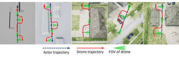
Figure 36: Drone trajectories of the highest rated policies in the user study in scenes 1 to 5.

The main perceived difference between the handcrafted reward policy and the human reward policy was the consistency of switching shots. While the former tries to switch shots every 2 times steps ($12$s) if not disturbed by an obstacle, the latter is more irregular in timing. From the user studies it is evident that a more regular period that is neither too short nor too long improves aesthetic scores.

9.4.3 Extended results in field experiments

We tested our trained policies in real-life settings. Since these tests were only focused on the shot selection module we operated using a pre-mapped environment, differently than the integrated results from Subsection 9.1 that uses online mapping. We filmed scenes using three distinct policies: one trained with handcrafted rewards on the BigMap environment, a second fixed back shot policy and a third random policy. Figure 37 summarizes the results.

Similar to the simulation results, the random policy results in constant loss of actor due to drastic position changes and close proximity to obstacles. For example, a random action of right shot will cause the UAV to climb much above the actor if it is too close to a large mound. The back shot policy, although stable in vehicle behavior, results in visually unappealing movies. Finally, our trained policy provides a middle ground, resulting in periodic changes in UAV viewpoint, while providing stable visual tracking.

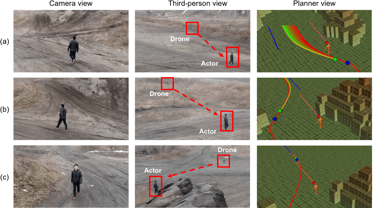
Figure 37: UAV follows an actor while switching shot types autonomously with our trained policy: a) UAV starts at the back of the actor; b) The mound’s presence on the right side of the actor leads to a left shot selection; c) UAV switches to a frontal shot in the open area.

10 Discussion

In this section we discuss lessons learned throughout the development of our work, and also present comments on how our methods can be used with different types of sensors and UAV platforms.

10.1 Lessons Learned

During development of our autonomous aerial cinematographer platform we learned several lessons and gained insights into problem specificities, which we summarize below. We expect these lessons to not only be useful to researchers in the field of aerial vehicles, but also to generalize to other related areas.

Cascading errors can destabilize the robot:

Estimation errors in a module get amplified if used downstream in decision making. For example, we learned that jerky UAV movements lead to mis-registration of camera pose, which leads to poor actor detection. This in turn leads to poor actor prediction, which can be off by meters. Unlike previous works that operate under highly precise motion capture systems, in real scenarios we observe that controlling the camera orientation towards the position estimates causes the robot to completely lose the actor. To mitigate this effect, we chose to decouple motion planning, which uses the actor world projection estimates, from camera control, which uses only object detections on the current image as feedback. To validate the quality of both threads independently, we performed statistical performance evaluations, as seen throughout Section 9.

Long-range sensors are beneficial to planning performance:

The planner relies on the online map. Slow online map updates slow down the planner. This typically happens when the robot moves near large pockets of unknown areas, which triggers large updates for the TSDT. We learned that a relatively long range LiDAR sensor maps out a significantly larger area. Hence almost always, the area near the robot is mapped out fully and the planner does not have to wait for map updates to enter an unknown region. While our system used a relatively large map of $250\times 250\times 100$m, significantly faster mapping-planning frequencies could be achieved with the use of a smaller local map. Such change would likely be necessary with the use of shorter-range sensors like stereo pairs, which are common in commercial aircrafts due to their reduced price.

Semi-supervised methods can improve learning generalization:

While deep learning methods are ubiquitous in computer vision, they rely on massive amounts of labeled data due to the complexity of the model class. Moreover, these models do not generalize to varying data distributions. We learned that one can reduce sample complexity by enforcing regularization / additional structure. In our case, we enforce temporal continuity on the network output. We show that a combination of small labeled dataset for supervisory loss and a large unlabeled dataset for temporal continuity loss is enough to solve the problem. Exploring other regularization techniques such as consistency between different sensory modalities is also an interesting area to be investigated in the future.

Height estimate using IMU and barometer is not enough for long operations:

During extended vehicle operations (over $5-10$ minutes), we learned that the UAV’s height calculated by fusing IMU and barometer data drifts significantly, especially after large vertical maneuvers. Inaccurate height estimates degrade pointcloud registration, thereby degrading the overall system performance. In the future, we plan to use LiDAR or visual SLAM to provide more accurate 3D localization.

Real-world noise reduces transferability of the artistic policy trained in simulation:

The noise present in real-world testing conditions, in particular for the map registration and actor localization, affected the results generated by the policy that was trained purely in simulation using ground-truth data. Shot selection in simulation highly prioritized viewpoints that drew the UAV away from tall obstacles, while in deployment we observed that the drone avoided proximity to tall objects with a significantly smaller frequency. In the future we will consider artificially adding noise to simulations for better transferability, or training the artistic policy with a combination of simulated and real-life data.

10.2 Adapting Our Work to Different UAVs and Sensors

In this work we employed a long-range LiDAR sensor for mapping the environment, and a DJI M210 UAV as the base platform. Even though we used relatively standard robotics development platform and sensor, researchers and developers who work on problems similar to aerial cinematography may face different constraints in terms of payload capacity, vehicle size, sensor modalities and costs. We argue that our problem formulation can be easily extended to other contexts.

First, we argue that the LiDAR sensor used in the online mapping module (Section 6) can be replaced by other sensors. Stereo cameras and depth sensors, for example, can be light-weight and significantly cheaper alternatives. The incoming hits for the mapping pipeline can then be acquired by using each pixel from a depth image, or each match from the stereo pair. The main advantage of LiDAR is the relatively long range, in the order of hundreds of meters. When using lighter sensors, the developer needs to take into account the new sensor range in order to keep the UAV safe. They must consider the expected vehicle speed and the scale of obstacles in the environment, so that the planner can reason about obstacles far from the UAV’s current position.

In addition, our system architecture is platform-agnostic. Our methods can easily be adapted to smaller or potentially cheaper platforms. To do so, one only needs to care for the software interface between the trajectory controller and the aircraft’s internal attitude or velocity controller.

In the future, we hope to see our architecture extended to other UAV types: our framework is not constrained to uniquely multi-rotors. With the appropriate changes in the motion planner’s trajectory parametrization and cost functions, our pipeline can also be employed by fixed-wing or hybrid aircrafts. More generally, despite the lower path dimensionality, even ground robots can employ the same methodology for visually tracking dynamic targets.

11 Conclusion

In this work we presented a complete system for robust autonomous aerial cinematography in unknown, unstructured environments while following dynamic actors in unscripted scenes. Current approaches do not address all theoretical and practical challenges present in real-life operation conditions; instead, they rely on simplifying assumptions such as requiring ground truth actor position, using prior maps of the environment, or only following one shot type specified before flight. To solve the entirety of the aerial cinematography, our system revolves around two key ideas. First, we frame the filming task as an efficient cost optimization problem, which allows trajectories with long time horizons to be computed in real time, even under sensor noise. Second, instead of using hand-defined heuristics to guide the UAV’s motion, we approach the artistic decision-making problem as a learning problem that can directly use human feedback.

We developed a system with four modules that work in parallel. (1) A vision-based actor localization module with motion prediction. (2) A real-time incremental mapping algorithm using a long-range LiDAR sensor. (3) A real-time optimization-based motion planner that exploits covariant gradients to efficiently calculate safe trajectories with long time horizons while balancing artistic objectives and occlusion avoidance for arbitrary obstacle shapes. (4) Finally, a deep reinforcement learning policy for artistic viewpoint selection.

We offered extensive detailed experiments to evaluate the robustness and real-time performance of our system both in simulation and real-life scenarios. These experiments occur among a variety of terrain types, obstacle shapes, obstacle complexities, actor trajectories, actor types (i.e., people, cars, bikes) and shot types.

Based on our results, we identify several key directions for possible future work. One clear direction is the extension of our theory to multi-drone, multi-actor scenarios. This improvement can be achieved by the addition of new cost functions that penalize inter-drone collisions, inter-drone sight, and a metric for multi-actor coverage. In addition, multi-actor scenarios require a slight modification in the definition of artistic parameters that define the desired artistic shot for our motion planner. Another interesting direction to follow lies among the reconstruction of dynamic scenes. While systems such as the CMU PanOptic Studio [Joo et al., 2015] can precisely reconstruct scenes volumetrically in indoor and static scenarios, to our knowledge, no current system offers good volumetric reconstruction of dynamic scenes in natural environments in real-life conditions. Lastly, we envision further research in learning the artistic reasoning behind human choices. More broadly, as robotics evolves, autonomous agents are required to operate in a large variety of tasks in proximity to humans, where success is in great part measured by the ability of the robot to execute aesthetic and human-like behaviors. We identify important related areas to cinematography, such as autonomous driving and human-robot interaction, where fine nuances of human behavior modeling are important for the development of autonomous agents.

Acknowledgments

We thank Xiangwei Wang and Greg Armstrong for the assistance in field experiments and robot construction. Research presented in this paper was funded by Yamaha Motor Co., Ltd. under award #A019969.

Appendix A Derivations of planning cost functions

A.1 Smoothness cost

We can discretize Equation 8 to compute the smoothness for $\xi_{q}$:

$$J_{\mathrm{smooth}}\left(\xi_{q}\right)=\frac{1}{(n-1)}\frac{1}{2}\sum_{t=1}^{n-1}\left[\alpha_{0}\left|\frac{p_{t}-p_{t-1}}{\Delta t}\right|^{2}+\alpha_{1}\left|\frac{\dot{p_{t}}-\dot{p_{t-1}}}{\Delta t}\right|^{2}+\alpha_{2}\left|\frac{\ddot{p_{t}}-\ddot{p_{t-1}}}{\Delta t}\right|^{2}+\dots\right]$$ (23)

To simplify Equation 23, we define: $\Delta t=\frac{t_{f}}{n-1}$, a finite differentiation operator $K$, and an auxiliary matrix $e$ for the contour conditions:

$$K_{(n-1)\times(n-1)}=\begin{bmatrix}1&0&0&\cdots&0&0&0\\ -1&1&0&\cdots&0&0&0\\ 0&-1&1&\cdots&0&0&0\\ &&&\vdots&&&\\ 0&0&0&0\cdots&0&-1&1\end{bmatrix}\quad e_{(n-1)\times 3}=\begin{bmatrix}-p_{0x}&-p_{0y}&-p_{0z}\\ 0&0&0\\ \vdots&\vdots&\vdots\\ 0&0&0\end{bmatrix}$$ (24)

By manipulating the terms $K$, $e$, and $\Delta t$ we obtain the auxiliary terms:

$$K_{0}=\frac{K}{\Delta t},\quad e_{0}=\frac{e}{\Delta t}$$ (25)

$$K_{1}=\frac{K^{2}}{\Delta t^{2}},\quad e_{1}=\frac{Ke}{\Delta t^{2}}+\frac{\dot{e}}{\Delta t^{2}}$$

$$K_{2}=\frac{K^{3}}{\Delta t^{3}},\quad e_{2}=\frac{K^{2}e}{\Delta t^{3}}+\frac{K\dot{e}}{\Delta t^{3}}+\frac{\ddot{e}}{\Delta t^{3}}$$

$$A_{0}=K_{0}^{T}K_{0},\quad b_{0}=K_{0}^{T}e_{0},\quad c_{0}=e_{0}^{T}e_{0}$$ (26)

$$A_{1}=K_{1}^{T}K_{1},\quad b_{1}=K_{1}^{T}e_{1},\quad c_{1}=e_{1}^{T}e_{1}$$

$$A_{2}=K_{2}^{T}K_{1},\quad b_{2}=K_{2}^{T}e_{2},\quad c_{2}=e_{2}^{T}e_{2}$$

Finally, we can analytically write the smoothness cost as a quadratic objective:

$$J_{\mathrm{smooth}}\left(\xi_{q}\right) =\frac{1}{2(n-1)}Tr(\xi_{q}^{T}A_{\mathrm{smooth}}\xi_{q}+2\xi_{q}^{T}b_{\mathrm{smooth}}+c_{\mathrm{smooth}})$$ (27)

where: $$A_{\mathrm{smooth}}=\alpha_{0}A_{0}+\alpha_{1}A_{1}+\dots$$

$$b_{\mathrm{smooth}}=\alpha_{0}b_{0}+\alpha_{1}b_{1}+\dots$$

$$c_{\mathrm{smooth}}=\alpha_{0}c_{0}+\alpha_{1}c_{1}+\dots$$

Since $J_{\mathrm{smooth}}\left(\xi_{q}\right)$ is quadratic, we find analytic expressions for its gradient and Hessian. Note that the Hessian expression does not depend on the current trajectory, which is a property used serve to speed up the optimization algorithm described in Subsection 7.4:

$$\nabla J_{\mathrm{smooth}}\left(\xi_{q}\right) =\frac{1}{(n-1)}(A_{\mathrm{smooth}}\xi_{q}+b_{\mathrm{smooth}})$$ (28)

$$\nabla^{2}J_{\mathrm{smooth}}\left(\xi_{q}\right) =\frac{1}{(n-1)}A_{\mathrm{smooth}}$$

A.2 Shot quality cost

We can calculate $J_{\mathrm{shot}}$ in the discrete form:

$$J_{\mathrm{shot}}\left(\xi_{q},\xi_{a}\right)=\frac{1}{(n-1)}\frac{1}{2}\sum_{t=1}^{n}\left|p_{t}-p_{\mathrm{t\ shot}}\right|^{2}$$ (29)

By defining auxiliary matrices, we can also define a quadratic expression:

$$J_{\mathrm{shot}}\left(\xi_{q},\xi_{a}\right)=\frac{1}{2(n-1)}Tr(\xi_{q}^{T}A_{\mathrm{shot}}\xi_{q}+2\xi_{q}^{T}b_{\mathrm{shot}}+c_{\mathrm{shot}})$$ (30)

where:

$$K_{\mathrm{shot}}=-I_{(n-1)\times(n-1)}$$ (31)

$$e_{\mathrm{shot}}=\xi_{\mathrm{shot}}=\begin{bmatrix}p_{\mathrm{1x\ shot}}&p_{\mathrm{1y\ shot}}&p_{\mathrm{1z\ shot}}\\ p_{\mathrm{1x\ shot}}&p_{\mathrm{1y\ shot}}&p_{\mathrm{1z\ shot}}\\ \vdots&\vdots&\vdots\\ p_{\mathrm{(n-1)x\ shot}}&p_{\mathrm{(n-1)y\ shot}}&p_{\mathrm{(n-1)z\ shot}}\\ \end{bmatrix},$$

and:

$$A_{\mathrm{shot}}=K_{\mathrm{shot}}^{T}K_{\mathrm{shot}},\quad b_{\mathrm{shot}}=K^{T}e_{\mathrm{shot}},\quad c_{\mathrm{shot}}=e_{\mathrm{shot}}^{T}e_{\mathrm{shot}}$$ (32)

We can again find analytic expressions for the shot quality gradient and Hessian, which is independent from the current trajectory:

$$\nabla J_{\mathrm{shot}}\left(\xi_{q}\right) =\frac{1}{(n-1)}(A_{\mathrm{shot}}\xi_{q}+b_{\mathrm{shot}})$$ (33)

$$\nabla^{2}J_{\mathrm{shot}}\left(\xi_{q}\right) =\frac{1}{(n-1)}A_{\mathrm{shot}}$$

References

- Aine et al., 2016 Aine, S., Swaminathan, S., Narayanan, V., Hwang, V., and Likhachev, M. (2016). Multi-heuristic a. The International Journal of Robotics Research, 35(1-3):224–243.
- Arijon, 1976 Arijon, D. (1976). Grammar of the film language.
- Bonatti et al., 2019 Bonatti, R., Ho, C., Wang, W., Choudhury, S., and Scherer, S. (2019). Towards a robust aerial cinematography platform: Localizing and tracking moving targets in unstructured environments. 2019 IEEE/RSJ International Conference on Intelligent Robots and Systems (IROS).
- Bonatti et al., 2018 Bonatti, R., Zhang, Y., Choudhury, S., Wang, W., and Scherer, S. (2018). Autonomous drone cinematographer: Using artistic principles to create smooth, safe, occlusion-free trajectories for aerial filming. International Symposium on Experimental Robotics.
- Bowen and Thompson, 2013 Bowen, C. J. and Thompson, R. (2013). Grammar of the Shot. Taylor & Francis.
- Boyd and Vandenberghe, 2004 Boyd, S. and Vandenberghe, L. (2004). Convex optimization. Cambridge university press.
- Cao et al., 2017 Cao, Z., Simon, T., Wei, S.-E., and Sheikh, Y. (2017). Realtime multi-person 2d pose estimation using part affinity fields. In CVPR.
- Charrow et al., 2015 Charrow, B., Kahn, G., Patil, S., Liu, S., Goldberg, K., Abbeel, P., Michael, N., and Kumar, V. (2015). Information-theoretic planning with trajectory optimization for dense 3d mapping. In Robotics: Science and Systems, volume 11. Rome.
- Choi et al., 2016 Choi, J., Lee, B.-J., and Zhang, B.-T. (2016). Human body orientation estimation using convolutional neural network. arXiv preprint arXiv:1609.01984.
- Choudhury et al., 2016 Choudhury, S., Gammell, J. D., Barfoot, T. D., Srinivasa, S. S., and Scherer, S. (2016). Regionally accelerated batch informed trees (rabit*): A framework to integrate local information into optimal path planning. In 2016 IEEE International Conference on Robotics and Automation (ICRA), pages 4207–4214. IEEE.
- Christiano et al., 2017 Christiano, P. F., Leike, J., Brown, T., Martic, M., Legg, S., and Amodei, D. (2017). Deep reinforcement learning from human preferences. In Advances in Neural Information Processing Systems, pages 4299–4307.
- Christie et al., 2008 Christie, M., Olivier, P., and Normand, J.-M. (2008). Camera control in computer graphics. In Computer Graphics Forum, volume 27, pages 2197–2218. Wiley Online Library.
- Cover et al., 2013 Cover, H., Choudhury, S., Scherer, S., and Singh, S. (2013). Sparse tangential network (spartan): Motion planning for micro aerial vehicles. In 2013 IEEE International Conference on Robotics and Automation, pages 2820–2825. IEEE.
- Dai et al., 2017 Dai, Z., Yang, Z., Yang, F., Cohen, W. W., and Salakhutdinov, R. R. (2017). Good semi-supervised learning that requires a bad gan. In Advances in Neural Information Processing Systems, pages 6513–6523.
- De-Miguel-Molina, 2018 De-Miguel-Molina, M. (2018). Ethics and Civil Drones: European Policies and Proposals for the Industry. Springer.
- Deng et al., 2017 Deng, Z., Si, W., Qu, Z., Liu, X., and Na, Z. (2017). Heading estimation fusing inertial sensors and landmarks for indoor navigation using a smartphone in the pocket. EURASIP Journal on Wireless Communications and Networking, 2017(1):160.
- DJI, 2018 DJI (2018). Dji mavic, https://www.dji.com/mavic.
- Drucker and Zeltzer, 1994 Drucker, S. M. and Zeltzer, D. (1994). Intelligent camera control in a virtual environment. In Graphics Interface, pages 190–190.
- Elbanhawi and Simic, 2014 Elbanhawi, M. and Simic, M. (2014). Sampling-based robot motion planning: A review. IEEE Access, (2):56–77.
- Fang and Zhang, 2017 Fang, H. and Zhang, M. (2017). Creatism: A deep-learning photographer capable of creating professional work. arXiv preprint arXiv:1707.03491.
- Flohr et al., 2015 Flohr, F., Dumitru-Guzu, M., Kooij, J. F., and Gavrila, D. M. (2015). A probabilistic framework for joint pedestrian head and body orientation estimation. IEEE Transactions on Intelligent Transportation Systems, 16(4):1872–1882.
- Galvane et al., 2017 Galvane, Q., Fleureau, J., Tariolle, F.-L., and Guillotel, P. (2017). Automated cinematography with unmanned aerial vehicles. arXiv preprint arXiv:1712.04353.
- Galvane et al., 2018 Galvane, Q., Lino, C., Christie, M., Fleureau, J., Servant, F., Tariolle, F., Guillotel, P., et al. (2018). Directing cinematographic drones. ACM Transactions on Graphics (TOG), 37(3):34.
- Gatys et al., 2016 Gatys, L. A., Ecker, A. S., and Bethge, M. (2016). Image style transfer using convolutional neural networks. In Proceedings of the IEEE Conference on Computer Vision and Pattern Recognition, pages 2414–2423.
- Gebhardt et al., 2016 Gebhardt, C., Hepp, B., Nägeli, T., Stevšić, S., and Hilliges, O. (2016). Airways: Optimization-based planning of quadrotor trajectories according to high-level user goals. In Proceedings of the 2016 CHI Conference on Human Factors in Computing Systems, pages 2508–2519. ACM.
- Gebhardt et al., 2018 Gebhardt, C., Stevšić, S., and Hilliges, O. (2018). Optimizing for aesthetically pleasing qadrotor camera motion. ACM Transactions on Graphics (TOG), 37(4):90.
- Geiger et al., 2013 Geiger, A., Lenz, P., Stiller, C., and Urtasun, R. (2013). Vision meets robotics: The kitti dataset. International Journal of Robotics Research (IJRR).
- Gleicher and Witkin, 1992 Gleicher, M. and Witkin, A. (1992). Through-the-lens camera control. In ACM SIGGRAPH Computer Graphics, volume 26, pages 331–340. ACM.
- Goroshin et al., 2015 Goroshin, R., Bruna, J., Tompson, J., Eigen, D., and LeCun, Y. (2015). Unsupervised learning of spatiotemporally coherent metrics. In Proceedings of the IEEE international conference on computer vision, pages 4086–4093.
- Gschwindt et al., 2019 Gschwindt, M., Camci, E., Bonatti, R., Wang, W., and Scherer, S. (2019). Can a robot become a movie director? learning artistic principles for aerial cinematography. 2019 IEEE/RSJ International Conference on Intelligent Robots and Systems (IROS).
- Henriques et al., 2015 Henriques, J. F., Caseiro, R., Martins, P., and Batista, J. (2015). High-speed tracking with kernelized correlation filters. IEEE Transactions on Pattern Analysis and Machine Intelligence, 37(3):583–596.
- Hoffer and Ailon, 2016 Hoffer, E. and Ailon, N. (2016). Semi-supervised deep learning by metric embedding. arXiv preprint arXiv:1611.01449.
- Howard et al., 2017 Howard, A. G., Zhu, M., Chen, B., Kalenichenko, D., Wang, W., Weyand, T., Andreetto, M., and Adam, H. (2017). Mobilenets: Efficient convolutional neural networks for mobile vision applications. arXiv preprint arXiv:1704.04861.
- Huang et al., 2018a Huang, C., Gao, F., Pan, J., Yang, Z., Qiu, W., Chen, P., Yang, X., Shen, S., and Cheng, K.-T. T. (2018a). Act: An autonomous drone cinematography system for action scenes. In 2018 IEEE International Conference on Robotics and Automation (ICRA), pages 7039–7046. IEEE.
- Huang et al., 2018b Huang, C., Yang, Z., Kong, Y., Chen, P., Yang, X., and Cheng, K.-T. T. (2018b). Through-the-lens drone filming. In 2018 IEEE/RSJ International Conference on Intelligent Robots and Systems (IROS), pages 4692–4699. IEEE.
- Huber et al., 1964 Huber, P. J. et al. (1964). Robust estimation of a location parameter. The annals of mathematical statistics, 35(1):73–101.
- Ionescu et al., 2014 Ionescu, C., Papava, D., Olaru, V., and Sminchisescu, C. (2014). Human3.6m: Large scale datasets and predictive methods for 3d human sensing in natural environments. IEEE Transactions on Pattern Analysis and Machine Intelligence, 36(7):1325–1339.
- Isler et al., 2016 Isler, S., Sabzevari, R., Delmerico, J., and Scaramuzza, D. (2016). An information gain formulation for active volumetric 3d reconstruction. In 2016 IEEE International Conference on Robotics and Automation (ICRA), pages 3477–3484. IEEE.
- Joo et al., 2015 Joo, H., Liu, H., Tan, L., Gui, L., Nabbe, B., Matthews, I., Kanade, T., Nobuhara, S., and Sheikh, Y. (2015). Panoptic studio: A massively multiview system for social motion capture. In Proceedings of the IEEE International Conference on Computer Vision, pages 3334–3342.
- Joubert et al., 2016 Joubert, N., Goldman, D. B., Berthouzoz, F., Roberts, M., Landay, J. A., Hanrahan, P., et al. (2016). Towards a drone cinematographer: Guiding quadrotor cameras using visual composition principles. arXiv preprint arXiv:1610.01691.
- Joubert et al., 2015 Joubert, N., Roberts, M., Truong, A., Berthouzoz, F., and Hanrahan, P. (2015). An interactive tool for designing quadrotor camera shots. ACM Transactions on Graphics (TOG), 34(6):238.
- Karaman and Frazzoli, 2011 Karaman, S. and Frazzoli, E. (2011). Sampling-based algorithms for optimal motion planning. The international journal of robotics research, 30(7):846–894.
- Karpathy, 2015 Karpathy, A. (2015). What a deep neural network thinks about your #selfie, andrej karpathy blog. karpathy. github. io.
- Kingma and Ba, 2014 Kingma, D. P. and Ba, J. (2014). Adam: A method for stochastic optimization. arXiv preprint arXiv:1412.6980.
- Kitani et al., 2012 Kitani, K. M., Ziebart, B. D., Bagnell, J. A., and Hebert, M. (2012). Activity forecasting. In European Conference on Computer Vision, pages 201–214. Springer.
- Klingensmith et al., 2015 Klingensmith, M., Dryanovski, I., Srinivasa, S., and Xiao, J. (2015). Chisel: Real time large scale 3d reconstruction onboard a mobile device using spatially hashed signed distance fields. In Robotics: Science and Systems, volume 4.
- Krishnamurthy et al., 2016 Krishnamurthy, A., Agarwal, A., and Langford, J. (2016). Contextual-mdps for pacreinforcement learning with rich observations. arXiv preprint arXiv:1602.02722.
- Kuffner and LaValle, 2000 Kuffner, J. and LaValle, S. (2000). Rrt-connect: An efficient approach to single-query path planning. In Proceedings 2000 ICRA. Millennium Conference. IEEE International Conference on Robotics and Automation. Symposia Proceedings (Cat. No. 00CH37065), volume 2, pages 995–1001. IEEE.
- La Bella, 2016 La Bella, L. (2016). Drones and Entertainment. The Rosen Publishing Group, Inc.
- Lan et al., 2017 Lan, Z., Shridhar, M., Hsu, D., and Zhao, S. (2017). Xpose: Reinventing user interaction with flying cameras. In Robotics: Science and Systems.
- LaValle, 2006 LaValle, S. M. (2006). Planning Algorithms. Cambridge University Press, Cambridge, U.K. Available at http://planning.cs.uiuc.edu/.
- Leake et al., 2017 Leake, M., Davis, A., Truong, A., and Agrawala, M. (2017). Computational video editing for dialogue-driven scenes. ACM Trans. Graph., 36(4):130–1.
- Lin et al., 2014 Lin, T.-Y., Maire, M., Belongie, S., Hays, J., Perona, P., Ramanan, D., Dollár, P., and Zitnick, C. L. (2014). Microsoft coco: Common objects in context. In European conference on computer vision, pages 740–755. Springer.
- Lino and Christie, 2015 Lino, C. and Christie, M. (2015). Intuitive and efficient camera control with the toric space. ACM Transactions on Graphics (TOG), 34(4):82.
- Lino et al., 2011 Lino, C., Christie, M., Ranon, R., and Bares, W. (2011). The director’s lens: an intelligent assistant for virtual cinematography. In Proceedings of the 19th ACM international conference on Multimedia, pages 323–332. ACM.
- Liu et al., 2016a Liu, D., Pei, L., Qian, J., Wang, L., Liu, P., Dong, Z., Xie, S., and Wei, W. (2016a). A novel heading estimation algorithm for pedestrian using a smartphone without attitude constraints. In Ubiquitous Positioning, Indoor Navigation and Location Based Services (UPINLBS), 2016 Fourth International Conference on, pages 29–37. IEEE.
- Liu et al., 2017 Liu, P., Liu, W., and Ma, H. (2017). Weighted sequence loss based spatial-temporal deep learning framework for human body orientation estimation. In Multimedia and Expo (ICME), 2017 IEEE International Conference on, pages 97–102. IEEE.
- Liu et al., 2016b Liu, W., Anguelov, D., Erhan, D., Szegedy, C., Reed, S., Fu, C.-Y., and Berg, A. C. (2016b). Ssd: Single shot multibox detector. In European conference on computer vision, pages 21–37. Springer.
- Liu et al., 2013 Liu, W., Zhang, Y., Tang, S., Tang, J., Hong, R., and Li, J. (2013). Accurate estimation of human body orientation from rgb-d sensors. IEEE Transactions on Cybernetics, 43(5):1442–1452.
- Luna et al., 2013 Luna, R., Şucan, I. A., Moll, M., and Kavraki, L. E. (2013). Anytime solution optimization for sampling-based motion planning. In 2013 IEEE international conference on robotics and automation, pages 5068–5074. IEEE.
- Mnih et al., 2013 Mnih, V., Kavukcuoglu, K., Silver, D., Graves, A., Antonoglou, I., Wierstra, D., and Riedmiller, M. (2013). Playing atari with deep reinforcement learning. arXiv preprint arXiv:1312.5602.
- Mnih et al., 2015 Mnih, V., Kavukcuoglu, K., Silver, D., Rusu, A. A., Veness, J., Bellemare, M. G., Graves, A., Riedmiller, M., Fidjeland, A. K., Ostrovski, G., et al. (2015). Human-level control through deep reinforcement learning. Nature, 518(7540):529.
- Mobahi et al., 2009 Mobahi, H., Collobert, R., and Weston, J. (2009). Deep learning from temporal coherence in video. In Proceedings of the 26th Annual International Conference on Machine Learning, pages 737–744. ACM.
- Nägeli et al., 2017 Nägeli, T., Meier, L., Domahidi, A., Alonso-Mora, J., and Hilliges, O. (2017). Real-time planning for automated multi-view drone cinematography. ACM Transactions on Graphics (TOG), 36(4):132.
- Nene et al., 1996 Nene, S. A., Nayar, S. K., Murase, H., et al. (1996). Columbia object image library (coil-20).
- Newcombe et al., 2011 Newcombe, R. A., Izadi, S., Hilliges, O., Molyneaux, D., Kim, D., Davison, A. J., Kohi, P., Shotton, J., Hodges, S., and Fitzgibbon, A. (2011). Kinectfusion: Real-time dense surface mapping and tracking. In Mixed and augmented reality (ISMAR), 2011 10th IEEE international symposium on, pages 127–136. IEEE.
- Oh et al., 2011 Oh, S., Hoogs, A., Perera, A., Cuntoor, N., Chen, C.-C., Lee, J. T., Mukherjee, S., Aggarwal, J., Lee, H., Davis, L., et al. (2011). A large-scale benchmark dataset for event recognition in surveillance video. In Computer vision and pattern recognition (CVPR), 2011 IEEE conference on, pages 3153–3160. IEEE.
- Oleynikova et al., 2016 Oleynikova, H., Taylor, Z., Fehr, M., Nieto, J., and Siegwart, R. (2016). Voxblox: Building 3d signed distance fields for planning. arXiv, pages arXiv–1611.
- Penin et al., 2018 Penin, B., Giordano, P. R., and Chaumette, F. (2018). Vision-based reactive planning for aggressive target tracking while avoiding collisions and occlusions. IEEE Robotics and Automation Letters, 3(4):3725–3732.
- Quigley et al., 2009 Quigley, M., Conley, K., Gerkey, B., Faust, J., Foote, T., Leibs, J., Wheeler, R., and Ng, A. Y. (2009). Ros: an open-source robot operating system. In ICRA workshop on open source software, volume 3, page 5. Kobe, Japan.
- Raman et al., 2016 Raman, R., Sa, P. K., Majhi, B., and Bakshi, S. (2016). Direction estimation for pedestrian monitoring system in smart cities: an hmm based approach. IEEE Access, 4:5788–5808.
- Rasmus et al., 2015 Rasmus, A., Berglund, M., Honkala, M., Valpola, H., and Raiko, T. (2015). Semi-supervised learning with ladder networks. In Advances in Neural Information Processing Systems, pages 3546–3554.
- Ratliff et al., 2009a Ratliff, N., Zucker, M., Bagnell, J. A., and Srinivasa, S. (2009a). CHOMP: Gradient optimization techniques for efficient motion planning. In Robotics and Automation, 2009. ICRA’09. IEEE International Conference on, pages 489–494. IEEE.
- Ratliff et al., 2009b Ratliff, N. D., Silver, D., and Bagnell, J. A. (2009b). Learning to search: Functional gradient techniques for imitation learning. Autonomous Robots, 27(1):25–53.
- Redmon et al., 2016 Redmon, J., Divvala, S., Girshick, R., and Farhadi, A. (2016). You only look once: Unified, real-time object detection. In Proceedings of the IEEE Conference on Computer Vision and Pattern Recognition, pages 779–788.
- Ren et al., 2015 Ren, S., He, K., Girshick, R., and Sun, J. (2015). Faster r-cnn: Towards real-time object detection with region proposal networks. In Advances in neural information processing systems, pages 91–99.
- Ristani et al., 2016 Ristani, E., Solera, F., Zou, R., Cucchiara, R., and Tomasi, C. (2016). Performance measures and a data set for multi-target, multi-camera tracking. In European Conference on Computer Vision workshop on Benchmarking Multi-Target Tracking.
- Roberts and Hanrahan, 2016 Roberts, M. and Hanrahan, P. (2016). Generating dynamically feasible trajectories for quadrotor cameras. ACM Transactions on Graphics (TOG), 35(4):61.
- Santamarina-Campos and Segarra-Oña, 2018 Santamarina-Campos, V. and Segarra-Oña, M. (2018). Introduction to drones and technology applied to the creative industry. airt project: An overview of the main results and actions. In Drones and the Creative Industry, pages 1–17. Springer.
- Schulman et al., 2013 Schulman, J., Ho, J., Lee, A., Awwal, I., Bradlow, H., and Abbeel, P. (2013). Finding locally optimal, collision-free trajectories with sequential convex optimization. In Robotics: Science and Systems, volume 9, pages 1–10.
- Shah et al., 2018 Shah, S., Dey, D., Lovett, C., and Kapoor, A. (2018). Airsim: High-fidelity visual and physical simulation for autonomous vehicles. In Field and service robotics, pages 621–635. Springer.
- Skydio, 2018 Skydio (2018). Skydio r1 self-flying camera, https://www.skydio.com/technology/.
- Soomro et al., 2012 Soomro, K., Zamir, A. R., and Shah, M. (2012). Ucf101: A dataset of 101 human actions classes from videos in the wild. arXiv preprint arXiv:1212.0402.
- Srivastava et al., 2015 Srivastava, N., Mansimov, E., and Salakhudinov, R. (2015). Unsupervised learning of video representations using lstms. In International conference on machine learning, pages 843–852.
- Stavens and Thrun, 2010 Stavens, D. and Thrun, S. (2010). Unsupervised learning of invariant features using video. In Computer Vision and Pattern Recognition (CVPR), 2010 IEEE Conference on, pages 1649–1656. IEEE.
- Strigel et al., 2014 Strigel, E., Meissner, D., Seeliger, F., Wilking, B., and Dietmayer, K. (2014). The ko-per intersection laserscanner and video dataset. In 17th International IEEE Conference on Intelligent Transportation Systems (ITSC), pages 1900–1901. IEEE.
- Sutton and Barto, 1998 Sutton, R. S. and Barto, A. G. (1998). Reinforcement learning: An introduction, volume 1. MIT press Cambridge.
- Thrun et al., 2005 Thrun, S., Burgard, W., and Fox, D. (2005). Probabilistic robotics. MIT press.
- Tian et al., 2014 Tian, R., Li, L., Yang, K., Chien, S., Chen, Y., and Sherony, R. (2014). Estimation of the vehicle-pedestrian encounter/conflict risk on the road based on tasi 110-car naturalistic driving data collection. In Intelligent Vehicles Symposium Proceedings, 2014 IEEE, pages 623–629. IEEE.
- Toshev and Szegedy, 2014 Toshev, A. and Szegedy, C. (2014). Deeppose: Human pose estimation via deep neural networks. In Proceedings of the IEEE conference on computer vision and pattern recognition, pages 1653–1660.
- Urmson et al., 2008 Urmson, C., Anhalt, J., Bagnell, D., Baker, C., Bittner, R., Clark, M., Dolan, J., Duggins, D., Galatali, T., Geyer, C., et al. (2008). Autonomous driving in urban environments: Boss and the urban challenge. Journal of Field Robotics, 25(8):425–466.
- Vázquez et al., 2015 Vázquez, M., Steinfeld, A., and Hudson, S. E. (2015). Parallel detection of conversational groups of free-standing people and tracking of their lower-body orientation. In Intelligent Robots and Systems (IROS), 2015 IEEE/RSJ International Conference on, pages 3010–3017. IEEE.
- Vista et al., 2015 Vista, F. P., Lee, D.-J., and Chong, K. T. (2015). Design of an ekf-ci based sensor fusion for robust heading estimation of marine vehicle. International Journal of Precision Engineering and Manufacturing, 16(2):403–407.
- Wang et al., 2016 Wang, C., Fang, Y., Zhao, H., Guo, C., Mita, S., and Zha, H. (2016). Probabilistic inference for occluded and multiview on-road vehicle detection. IEEE Transactions on Intelligent Transportation Systems, 17(1):215–229.
- Wang et al., 2019 Wang, W., Ahuja, A., Zhang, Y., Bonatti, R., and Scherer, S. (2019). Improved generalization of heading direction estimation for aerial filming using semi-supervised regression. Robotics and Automation (ICRA), 2019 IEEE International Conference on.
- Wang and Gupta, 2015 Wang, X. and Gupta, A. (2015). Unsupervised learning of visual representations using videos. In Proceedings of the 2015 IEEE International Conference on Computer Vision (ICCV), pages 2794–2802. IEEE Computer Society.
- Weston et al., 2012 Weston, J., Ratle, F., Mobahi, H., and Collobert, R. (2012). Deep learning via semi-supervised embedding. In Neural Networks: Tricks of the Trade, pages 639–655. Springer.
- Wu et al., 2018 Wu, H.-Y., Palù, F., Ranon, R., and Christie, M. (2018). Thinking like a director: Film editing patterns for virtual cinematographic storytelling. ACM Transactions on Multimedia Computing, Communications, and Applications (TOMM), 14(4):81.
- Xie et al., 2018 Xie, K., Yang, H., Huang, S., Lischinski, D., Christie, M., Xu, K., Gong, M., Cohen-Or, D., and Huang, H. (2018). Creating and chaining camera moves for quadrotor videography. ACM Transactions on Graphics, 37:14.
- Zhang et al., 2018 Zhang, Y., Wang, W., Bonatti, R., Maturana, D., and Scherer, S. (2018). Integrating kinematics and environment context into deep inverse reinforcement learning for predicting off-road vehicle trajectories. In Conference on Robot Learning, pages 894–905.
- Zou et al., 2012 Zou, W., Zhu, S., Yu, K., and Ng, A. Y. (2012). Deep learning of invariant features via simulated fixations in video. In Advances in neural information processing systems, pages 3203–3211.
- Zucker et al., 2013 Zucker, M., Ratliff, N., Dragan, A. D., Pivtoraiko, M., Klingensmith, M., Dellin, C. M., Bagnell, J. A., and Srinivasa, S. S. (2013). CHOMP: Covariant hamiltonian optimization for motion planning. The International Journal of Robotics Research, 32(9-10):1164–1193.