Some Geometric Applications of Anti-Chains

Abstract

We present an algorithmic framework for computing anti-chains of maximum size in geometric posets. Specifically, posets in which the entities are geometric objects, where comparability of two entities is implicitly defined but can be efficiently tested. Computing the largest anti-chain in a poset can be done in polynomial time via maximum-matching in a bipartite graph, and this leads to several efficient algorithms for the following problems, each running in (roughly) $O(n^{3/2})$ time:

1. Computing the largest Pareto-optimal subset of a set of $n$ points in $\mathbb{R}^{d}$.

2. Given a set of disks in the plane, computing the largest subset of disks such that no disk contains another. This is quite surprising, as the independent version of this problem is computationally hard.

3. Given a set of axis-aligned rectangles, computing the largest subset of non-crossing rectangles.

1 Introduction

Partial orderings.

Let $\left({V,\prec}\right)$ be a partially ordered set (or a poset), where $V$ is a set of entities. An anti-chain is a subset of elements $D\subseteq V$ such that all pairs of elements in $D$ are incomparable in $\left({V,\prec}\right)$. A chain is a subset $C\subseteq V$ such that all pairs of elements in $C$ are comparable. A chain cover $\mathcal{C}$ is a collection of chains whose union covers $V$. Observe that any anti-chain can contain at most one element from any given chain. As such, if $\mathcal{C}$ is the smallest collection of chains covering $V$, then for any anti-chain $D$, $\left|{D}\right|\leq\left|{\mathcal{C}}\right|$. Dilworth’s Theorem [Dil50] states that the minimum number of chains whose union covers $V$ is equal to the anti-chain of maximum size.

Implicit posets arising from geometric problems.

We are interested in implicitly defined posets, where the elements of the poset are geometric objects. In particular, if one can compute the largest anti-chain in these implicit posets, we obtain algorithms solving natural geometric problems. To this end, we describe a framework for computing anti-chains in an implicitly defined poset $\left({V,\prec}\right)$, under the following two assumptions: (i) comparability of two elements in the poset can be efficiently tested, and (ii) given an element $v\in V$, one can quickly find an element $u\in V$ with $v\prec u$.

As an example, let $P$ be a set of $n$ points in the plane. Form the partial ordering $\left({P,\prec}\right)$, where $q\prec p$ if $p$ dominates $q$. One can efficiently test comparability of two points, and given $q$, can determine if it is dominated by a point $p$ by reducing the problem to an orthogonal range query. Observe that an anti-chain in $\left({P,\prec}\right)$ corresponds to a collection of points in which no point dominates another. The largest such subset can be computed efficiently by finding the largest anti-chain in $\left({P,\prec}\right)$, see Lemma 3.2.

Previous work.

Posets have been previously utilized and studied in computational geometry [SK98, FW98, MW92]. For the poset $\left({P,\prec}\right)$ described above, Felsner and Wernisch [FW98] study the problem of computing the largest subset of points which can be covered by $k$-antichains.

Our results.

We describe a general framework for computing anti-chains in posets defined implicitly, see Theorem 2.4. As a consequence, we have the following applications:

1. Largest Pareto-optimal subset. Let $P\subseteq\mathbb{R}^{d}$ be a set of $n$ points. A point $p\in\mathbb{R}^{d}$ dominates a point $q\in\mathbb{R}^{d}$ if $p\geq q$ coordinate wise. Compute the largest subset of points $S\subseteq P$, so that no point in $S$ dominates any other point in $S$. In two dimensions this corresponds to computing the longest downward “staircase”, which can be done in $O(n\log n)$ time (our algorithm is not interesting in this case). However, for three and higher dimensions, it corresponds to a surface of points that form the largest Pareto-optimal subset of the given point set.

2. Largest loose subset. Let $\mathcal{D}$ be a set of $n$ regions in $\mathbb{R}^{d}$. A subset $S\subseteq\mathcal{D}$ is loose if for every pair $\mathsf{d}_{1},\mathsf{d}_{2}\in S$, $\mathsf{d}_{1}\not\subseteq\mathsf{d}_{2}$ and $\mathsf{d}_{2}\not\subseteq\mathsf{d}_{1}$. This is a weaker concept than independence, which requires that no pair of objects intersect. Surprisingly, computing the largest loose set can be done in polynomial time, as it reduces to finding the largest anti-chain in a poset. Compare this to the independent set problem, which is NP-Hard for all natural shapes in the plane (triangles, rectangles, disks, etc).

3. Largest subset of non-crossing rectangles. Let $\mathcal{R}$ be a set of $n$ axis-aligned rectangles in the plane. Compute the largest subset of rectangles $S\subseteq\mathcal{R}$, such that every pair of rectangles in $S$ intersect at most twice. Equivalently, $S$ is non-crossing, or $S$ forms a collection of pseudo-disks.

4. Largest isolated subset of points. Let $L$ be a collection lines in the plane (not necessarily in general position), and let $P$ be a set of points lying on the lines of $L$. A point $p\in P$ can reach a point $q\in P$ if $p$ can travel from left to right, along the lines of $L$, to $q$. A subset of points $Q\subseteq P$ are isolated if no point in $Q$ can reach any other point in $Q$ using the lines $L$, see Figure 1.1.

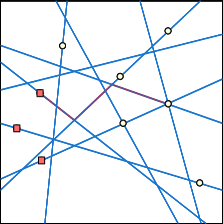
Figure 1.1: Left: A set of points on lines. Middle: A point reaching another. Right: An isolated subset.

Our results are summarized in Table 1.1.

Computing largest subset of	Entities	Running time	Ref
Pareto-optimal	Points in $\mathbb{R}^{d}$, $d>2$	$\scalerel*{\widetilde{O}}{j^{2}}(n^{1.5})\Bigr{.}$	Lemma 3.2
Loose	Arbitrary regions in $\mathbb{R}^{d}$	$O(n^{2.5})\Bigr{.}$	Lemma 3.6
	Arbitrary regions in $\mathbb{R}^{d}$ with a dynamic range searching data structure, $Q(n)$ time per operation	$O(n^{1.5}Q(n))\Bigr{.}$	Lemma 3.7
	Disks in the plane	$\scalerel*{\widetilde{O}}{j^{2}}(n^{1.5})\Bigr{.}$	Corollary 3.9
Non-crossing	Axis aligned rectangles in $\mathbb{R}^{2}$	$\scalerel*{\widetilde{O}}{j^{2}}(n^{1.5})\Bigr{.}$	Lemma 3.12
Isolated	Points on lines in $\mathbb{R}^{2}$	$O(n^{3})$	Lemma 3.14

Table 1.1: Our results, where $\widetilde{O}$ hides factors of the form $\log^{c}n$ ($c$ may depend on $d$).

2 Framework

2.1 Computing anti-chains

The following is a constructive proof of Dilworth’s Theorem from the max-flow min-cut Theorem, and is of course well known [Sch03]. We provide a proof for the sake of completeness.

Lemma 2.1.

Let $\left({V,\prec}\right)$ be a poset. Assume that comparability of two elements can be checked in $O(1)$ time. Then a maximum size anti-chain in $\left({V,\prec}\right)$ can be computed in $O(n^{2.5})$ time.

Proof:

Given $\left({V,\prec}\right)$, construct the bipartite graph $G=(U,E)$, where $U={{V}^{-}}\cup{{V}^{+}}$ and ${{V}^{-}}$, ${{V}^{+}}$ are copies of $V$. Add an edge $({{v}^{-}},{{u}^{+}})$ to $E$ when $v\prec u$ in $\left({V,\prec}\right)$. Next, compute the maximum matching in $G$ using the algorithm of Hopcroft-Karp [HK73], which runs in time $O\bigl{(}\left|{E}\right|\sqrt{\left|{U}\right|}\bigr{)}=O(n^{2.5})$. Let $M\subseteq E$ be the resulting maximum matching in $G$. Define ${{Q}^{-}}\subseteq{{U}^{-}}$ as the set of unmatched vertices. A path in $G$ is alternating if the edges of the path alternate between matched and unmatched edges. Let $S\subseteq{{V}^{-}}\cup{{V}^{+}}$ be the set of vertices which are members of alternating paths starting from any vertex in ${{Q}^{-}}$. Finally, set $D=\left\{v\in V\;\middle|\;{{v}^{-}}\in S,{{v}^{+}}\not\in S\right\}$. We claim $D$ is an anti-chain of maximum size.

Conceptually, suppose that $G$ is a directed network flow graph. Modify $G$ by adding two new vertices $s$ and $t$ and add the directed edges $(s,{{v}^{-}})$ and $({{v}^{+}},t)$, each with capacity one for all $v\in V$. Finally, direct all edges from ${{V}^{-}}$ to ${{V}^{+}}$ with infinite capacity. By the max-flow min-cut Theorem, the maximum matching $M$, induces a minimum $s$-$t$ cut, which is the cut $(s+S,t+U\setminus S)$, where $S$ is defined above. Indeed, $s+S$ is the reachable set from $s$ in the residual graph for $G$. To see why $D$ is an anti-chain, suppose that there exist two comparable elements $v,u\in D$. This implies that ${{v}^{-}},{{u}^{-}}\in S$ and ${{v}^{+}},{{u}^{+}}\notin S$. Assume without loss of generality that $v\prec u$. This implies that $({{v}^{-}},{{u}^{+}})$ is an edge of the network flow graph $G$ with infinite capacity that is in the cut $(s+S,V\setminus S+t)$. This contradicts the finiteness of the cut capacity.

We next prove that $\left|{D}\right|$ is maximum. Note that an element $v\in V$ is not in $D$ if ${{v}^{-}}\notin S$ or ${{v}^{+}}\in S$. If ${{v}^{-}}\notin S$ then $(s,{{v}^{-}})$ is in the cut. Similarly, if ${{v}^{+}}\in S$ then $({{v}^{+}},t)$ is in the cut. Since the minimum cut has capacity $\left|{M}\right|$, there are at most $\left|{M}\right|$ such vertices, which implies that $\left|{D}\right|\geq n-\left|{M}\right|$.

On the other hand, a chain cover $\mathcal{C}$ for $\left({V,\prec}\right)$ can be constructed from $M$. Given $\left({V,\prec}\right)$, create a DAG $H$ with vertex set $V$. We add the directed edge $(u,v)$ to $H$ when $u\prec v$. Now an edge $({{u}^{-}},{{v}^{+}})$ in $M$ corresponds to the edge $(u,v)$ of $H$. As such, a matching corresponds to a collection of edges in $H$, where every vertex appears at most twice. Since $H$ is a DAG, it follows that $M$ corresponds to a collection of paths in $H$. The end vertex $x$ of such a path corresponds to a vertex ${{x}^{-}}\in{{V}^{-}}$ that is unmatched (as otherwise, the path can be extended), and this is the only unmatched vertex on this path. There are at most $n-\left|{M}\right|$ unmatched vertices in ${{V}^{-}}$, which implies that $\left|{\mathcal{C}}\right|\leq n-\left|{M}\right|$. Hence, $D$ is an anti-chain with $\left|{D}\right|\geq n-\left|{M}\right|\geq\left|{\mathcal{C}}\right|$. Additionally, recall that for any anti-chain $D^{\prime}$, $\left|{D^{\prime}}\right|\leq\left|{\mathcal{C}}\right|$. These two inequalities imply that $D$ is of maximum possible size.  

Remark 2.2.

As described above, the edges of the matching $M$ correspond to a collection of edges in the DAG $H$. These edges together form a collection of vertex-disjoint paths which cover the vertices of $H$, and this is the minimum possible number of paths needed to cover the vertices.

2.2 Computing anti-chains on implicit posets

Here, we focus on computing anti-chains in posets, in which comparability of two elements are efficiently computable. Our main observation is that one can use range searching data structures to run the Hopcroft-Karp bipartite matching algorithm faster [HK73]. This observation goes back to the work of Efrat et al. [EIK01], where they study the problem of computing a perfect matching $M$ in a weighted bipartite graph $G$ such that the maximum weight edge in $M$ is minimized. They focus on solving the decision version of the problem: given a parameter $r$, is there a perfect matching $M$ with maximum edge weight at most $r$?

Theorem 2.3 ([EIK01, Theorem 3.2]).

Let $G$ be a bipartite graph on $n$ vertices with bipartition $A\cup B$, and $r>0$ a parameter. For any subset $U\subseteq B$ of $m$ vertices, suppose one can construct a data structure $\mathcalb{D}\left({B}\right)$ such that:

1. Given a query vertex $v\in A$, $\mathcalb{D}\left({B}\right)$ returns a vertex $u\in B$ such that the wight of the edge $(u,v)$ is at most $r$ (or reports that no such element in $B$ exists) in $T(m)$ time.

2. An element of $B$ can be deleted from $\mathcalb{D}\left({B}\right)$ in $T(m)$ time.

3. $\mathcalb{D}\left({B}\right)$ can be constructed in $O\bigl{(}m\cdot T(m)\bigr{)}$ time.

Then one can decide if there is a perfect matching $M$ in $G$, such that all edges in $M$ have weight at most $r$, in $O\bigl{(}n^{1.5}\cdot T(n)\bigr{)}$ time.

Recently, Cabello and Mulzer [CM20] also use a similar framework as described above for computing minimum cuts in disk graphs in $\scalerel*{\widetilde{O}}{j^{2}}(n^{1.5})$ time. We show that the above framework can also be extended to computing anti-chains, with a small modification to the data structure requirements.

Theorem 2.4.

Let $\left({V,\prec}\right)$ be a poset, where $n=\left|{V}\right|$. For any subset $P\subseteq V$ of $m$ elements, suppose one can construct a data structure $\mathcalb{D}\left({P}\right)$ such that:

1. Given a query $v\in V$, $\mathcalb{D}\left({P}\right)$ returns an element $u\in P$ with $v\prec u$ (or reports that no such element in $P$ exists) in $T(m)$ time.

2. An element can be deleted from $\mathcalb{D}\left({P}\right)$ in $T(m)$ time.

3. $\mathcalb{D}\left({P}\right)$ can be constructed in $O\bigl{(}m\cdot T(m)\bigr{)}$ time.

Then one can compute the maximum size anti-chain for $\left({V,\prec}\right)$ in $O\bigl{(}n^{1.5}\cdot T(n)\bigr{)}$ time.

Proof:

Create the vertex set $U={{V}^{-}}\cup{{V}^{+}}$ of the bipartite graph $G=(U,E)$ associated with $\left({V,\prec}\right)$. The neighborhood of a vertex in the bipartite graph can be found by constructing and querying the data structure $\mathcalb{D}$. Recall that in each iteration of the maximum matching algorithm of Hopcroft-Karp [HK73], a BFS tree is computed in the residual network of $G$. Such a tree can be computed in $O(nT(n))$, as can be easily verified (the BFS algorithm is essentially described below). Furthermore, the algorithm terminates after $O(\sqrt{n})$ iterations, which implies that one can compute the maximum matching in $G$ in $O(n^{1.5}\cdot T(n))$ time. See Efrat et al. [EIK01] for details. Let $M$ be the matching computed.

By Lemma 2.1, computing the maximum anti-chain reduces to computing the set of vertices which can be reached by alternating paths originating from unmatched vertices in ${{V}^{-}}$. Call this set of vertices $S$, as in Lemma 2.1.

To compute $S$, we do a BFS in the residual network of $G$. To this end, build the data structure $\mathcalb{D}\left({{{V}^{+}}}\right)$. Start at an arbitrary unmatched vertex $v\in{{V}^{-}}$, add it to $S$, and query $\mathcalb{D}\left({{{V}^{+}}}\right)$ to travel to a neighbor $u\in{{V}^{+}}$ along an unmatched edge. Add $u$ to $S$ and delete $u$ from $\mathcalb{D}\left({{{V}^{+}}}\right)$. Travel back to a vertex $x$ in ${{V}^{-}}$ using an edge of the matching $M$ (if possible) and add $x$ to $S$. This process is iterated until the alternating path has been exhausted. Then, restart the search from $v$ (if $v$ has any remaining unmatched neighbors) or another unmatched vertex of ${{V}^{-}}$. Observe that each vertex in ${{V}^{+}}$ is inserted and deleted at most once from the data structure $\mathcalb{D}$. Furthermore, each query to $\mathcalb{D}$ can be charged to a vertex deletion. Hence, $S$ can be computed in $O(n\cdot T(n))$ time.

Given $S$, in $O(n)$ time we can compute a maximum anti-chain $D=\left\{v\in V\;\middle|\;{{v}^{-}}\in S,{{v}^{+}}\not\in S\right\}$.  

3 Applications

3.1 Largest Pareto-optimal subset of points

Definition 3.1.

Let $P$ be a set of points in $\mathbb{R}^{d}$. A point $p\in\mathbb{R}^{d}$ dominates a point $q\in\mathbb{R}^{d}$ if $p\geq q$ coordinate wise. The point set $P$ is Pareto-optimal if no point in $P$ dominates any other point in $P$.

Lemma 3.2.

Let $P\subset\mathbb{R}^{d}$ be a set of $n$ points. A Pareto-optimal subset of $P$ of maximum size can be computed in $O(n^{1.5}(\log n/\log\log n)^{d-1})$ time.

Proof:

Form the implicit poset $\left({P,\prec}\right)$ where $q\prec p$ $\iff$ $p$ dominates $q$. Hence, two elements are incomparable when neither is dominated by the other. As such, computing the largest Pareto-optimal subset is reduced to finding the maximum anti-chain in $\left({P,\prec}\right)$.

To apply Theorem 2.4, one needs to exhibit a data structure $\mathcalb{D}$ with the desired properties. For a given query $q$, finding a point $p\in P$ with $q\prec p$ corresponds to finding a point $p$ which dominates $q$. Equivalently, such a point in $P$ exists if and only if it lies in the range $[q_{1},\infty)\times\ldots\times[q_{d},\infty)$. This is a $d$-sided orthogonal range query. Chan and Tsakalidis’s dynamic data structure for orthogonal range searching [CT17] suffices—their data structure can handle deletions and queries in $T(n)=O((\log n/\log\log n)^{d-1})$ amortized time, and can be constructed in $O(n\cdot T(n))$ time.  

3.1.1 Chain decomposition

Let $P$ be a set of $n$ points in $\mathbb{R}^{d}$. We would like to decompose $P$ into disjoint chains of dominated points, such that all the points are covered, and the number of chains is minimum. By Remark 2.2, this can be done by running the algorithm Lemma 3.2, and converting the bipartite matching to chains. This would take $O(n^{1.5}(\log n/\log\log n)^{d-1})$ time.

As a concrete example, suppose we want to solve a more restricted problem in the planar case—decomposing a given point set into chains of points (that are monotone in both $x$ and $y$), such that no pair of chains intersect.

Suppose that we have computed a chain decomposition of the points $P$. Let $C_{1}$ and $C_{2}$ be two chains of points, each with an edge $p_{i}q_{i}$ in $C_{i}$ (and $p_{i}$ dominates $q_{i}$) for $i=1,2$ such that $p_{1}q_{1}$ and $p_{2}q_{2}$ intersect in the plane. An exchange argument shows that by deleting these two edges and adding the edges $p_{1}q_{2}$ to $C_{1}$ and $p_{2}q_{1}$ to $C_{2}$, we decrease the total length of the chains. Indeed, let $s$ be the intersection point of the edges $p_{1}q_{1}$ and $p_{2}q_{2}$. By the triangle inequality and assuming the points of $P$ are in general position,

$$\|p_{1}-q_{2}\|+\|p_{2}-q_{1}\|<\|p_{1}-s\|+\|s-q_{2}\|+\|p_{2}-s\|+\|s-q_{1}\|=\|p_{1}-q_{1}\|+\|p_{2}-q_{2}\|.$$

As such, suppose we assign a weight to each edge in the bipartite graph $G$ equal to the distance between the two corresponding points. If $k$ is the size of the maximum (unweighted) matching in $G$, then we can compute a matching of cardinality $k$ with minimum weight by solving a min-cost flow instance on $G$ (using the weights on the edges of $G$ as the costs). This implies that the resulting chain decomposition covers all points of $P$, and no pair of chains intersect. We obtain the following.

Lemma 3.3.

Let $P$ be a set of $n$ points in the plane in general position. In polynomial time, one can compute the minimum number of non-intersecting $(x,y)$-monotone polygonal curves covering the points of $P$, where every point of $P$ must be a vertex of one of these polygonal curves, and the vertices of the polygonal curves are points of $P$.

Remark 3.4.

If we do not require the collection of polygonal curves to be non-intersecting, there is a much simpler algorithm. Create a directed acyclic graph $H=(P,E)$, where $(p,q)\in E$ if $p$ dominates $q$. Observe that all of the points $S\subseteq P$ in $H$ with out-degree zero form a polygonal curve. We add this curve to our collection and recursively compute the set of curves on the residual graph $H\setminus S$. While the number of polygonal curves is minimum, the resulting curves may intersect.

3.2 Largest loose subset of regions

Definition 3.5.

Let $\mathcal{D}$ be a collection of $n$ regions in $\mathbb{R}^{d}$. Such a collection $\mathcal{D}$ is loose if no region of $\mathcal{D}$ is fully contained inside another region of $\mathcal{D}$.

Lemma 3.6.

Let $\mathcal{D}$ be a collection of $n$ regions in $\mathbb{R}^{d}$. Suppose that for any two regions in $\mathcal{D}$, we can test if one is contained inside the other in $O(1)$ time. Then the largest loose subset of $\mathcal{D}$ can be computed in $O(n^{2.5})$ time.

Proof:

Form the implicit poset $\left({\mathcal{D},\prec}\right)$, where $\mathsf{d}^{\prime}\prec\mathsf{d}$ $\iff$ the region $\mathsf{d}$ is contained in the interior of $\mathsf{d}^{\prime}$. In particular, a subset of regions are loose if and only if they form an anti-chain in $\left({\mathcal{D},\prec}\right)$.

By Lemma 2.1 (and the assumption that containment of objects can be tested in $O(1)$ time) the largest anti-chain, and thus the largest loose subset, can be computed in $O(n^{2.5})$ time.  

Lemma 3.7.

Let $\mathcal{D}$ be a collection of $n$ regions in $\mathbb{R}^{d}$. For any subset $R\subseteq\mathcal{D}$ of $m$ regions, suppose one can construct a data structure $\mathcalb{D}\left({R}\right)$ such that:

1. Given a query $\mathsf{d}\in\mathcal{D}$, $\mathcalb{D}\left({R}\right)$ returns a region $\mathsf{d}^{\prime}\in R$ with $\mathsf{d}^{\prime}\subseteq\mathsf{d}$ (or reports that no such region in $R$ exists) in $Q(m)$ time.

2. A region can be deleted from $\mathcalb{D}\left({R}\right)$ in $Q(m)$ time.

3. $\mathcalb{D}\left({R}\right)$ can be constructed in $O\bigl{(}m\cdot Q(m)\bigr{)}$ time.

Then one can compute the largest loose subset of $\mathcal{D}$ in $O\bigl{(}n^{1.5}\cdot Q(n)\bigr{)}$ time.

Proof:

The proof follows by considering the poset $\left({\mathcal{D},\prec}\right)$ described in Lemma 3.6 and applying Theorem 2.4 using the data structure $\mathcalb{D}$.  

3.2.1 Largest loose subset of disks

We show how to compute the largest loose subset when the regions are disks in the plane. To apply Lemma 3.7, we need to exhibit the required dynamic data structure $\mathcalb{D}$.

Lemma 3.8.

Let $\mathcal{D}$ be a set of $n$ disks in the plane. There is a dynamic data structure $\mathcalb{D}$, which given a query disk $\mathsf{q}$, can return a disk $\mathsf{d}^{\prime}\in\mathcal{D}$ such that $\mathsf{d}^{\prime}\subseteq\mathsf{q}$ (or report that so such disk exists) in $O(\log^{2}n)$ deterministic time. Insertion and deletion of disks cost $O(\log^{10+\varepsilon}n)$ amortized expected time, for all $\varepsilon>0$.

Proof:

Associate each disk $\mathsf{d}\in\mathcal{D}$, which has center $\mathsf{c}_{\mathsf{d}}$ and radius $r_{\mathsf{d}}$, with a weighted distance function $\delta_{\mathsf{d}}:\mathbb{R}^{2}\to\mathbb{R}$, where $\delta_{\mathsf{d}}\left({p}\right)=\left\|\mathsf{c}_{\mathsf{d}}-p\right\|+r_{\mathsf{d}}$. Observe that a disk $\mathsf{d}$ is contained inside the interior of a disk $\mathsf{q}$ if and only if $\delta_{\mathsf{d}}\left({\mathsf{c}_{\mathsf{q}}}\right)\leq r_{\mathsf{q}}$. For a query disk $\mathsf{q}$, our goal will be to compute $\arg\min_{\mathsf{d}\in\mathcal{D}}\delta_{\mathsf{d}}\left({\mathsf{c}_{\mathsf{q}}}\right)$. After finding such a disk $\mathsf{d}^{\prime}$, return that $\mathsf{d}^{\prime}\subseteq\mathsf{q}$ if and only if $\delta_{\mathsf{d}^{\prime}}\left({\mathsf{c}_{\mathsf{q}}}\right)\leq r_{\mathsf{q}}$.

Hence, the problem is reduced to dynamically maintaining the function $F(p)=\min_{\mathsf{d}\in\mathcal{D}}\delta_{\mathsf{d}}\left({p}\right)$, for all $p\in\mathbb{R}^{2}$, under insertions and deletions of disks. Equivalently, $F$ is also the lower envelope of the $xy$-monotone surfaces defined by $\left\{\delta_{\mathsf{d}}\;\middle|\;\mathsf{d}\in\mathcal{D}\right\}$ in $\mathbb{R}^{3}$. This problem was studied by Kaplan et al. [KMR⁺17]: They prove that if $F$ is defined by a collection of additively weighted Euclidean distance functions, then $F$ can be computed for a given query $p$ in $O(\log^{2}n)$ time. Furthermore, updates can be handled in $O\big{(}2^{O(\alpha(\log n)^{2})}\log^{10}n\big{)}$ time, where $\alpha(n)$ is the inverse Ackermann function.  

Corollary 3.9.

Let $\mathcal{D}$ be a set of $n$ disks in the plane. The largest loose subset of disks can be computed in $O(n^{1.5}\log^{10+\varepsilon}n)$ expected time, for all $\varepsilon>0$.

Proof:

Follows from Lemma 3.7 in conjunction with the data structure described in Lemma 3.8.  

Remark 3.10.

By Remark 2.2, one can decompose a given set of $n$ disks into the minimum number of disjoint towers, where each tower is a sequence of disks of the form $d_{1}\subseteq d_{2}\subseteq\cdots\subseteq d_{t}$. The resulting running time is as stated in Corollary 3.9.

3.3 Largest subset of non-crossing rectangles

Definition 3.11.

A collection $\mathcal{R}$ of axis-aligned rectangles are non-crossing if the boundaries of every pair of rectangles in $\mathcal{R}$ intersect at most twice.

Lemma 3.12.

Let $\mathcal{R}$ be a set of $n$ axis-aligned rectangles in the plane. A non-crossing subset of $\mathcal{R}$ of maximum size can be computed in $O(n^{1.5}(\log n/\log\log n)^{3})$ time.

Proof:

For each rectangle $R\in\mathcal{R}$, let $\mathsf{t}\left({R}\right)$ and $\mathsf{b}\left({R}\right)$ denote the $y$-coordinate of the top and bottom sides of $R$, respectively. Similarly, $\mathsf{l}\left({R}\right)$ and $\mathsf{r}\left({R}\right)$ denotes the $x$-coordinate for the left and right sides of $R$.

Form the poset $\left({\mathcal{R},\prec}\right)$ where

$$R^{\prime}\prec R\iff[\mathsf{l}\left({R}\right),\mathsf{r}\left({R}\right)]\subseteq[\mathsf{l}\left({R^{\prime}}\right),\mathsf{r}\left({R^{\prime}}\right)]\text{ and }[\mathsf{b}\left({R^{\prime}}\right),\mathsf{t}\left({R^{\prime}}\right)]\subseteq[\mathsf{b}\left({R}\right),\mathsf{t}\left({R}\right)].$$

Observe two rectangles $R$ and $R^{\prime}$ are incomparable if and only if the boundaries of $R$ and $R^{\prime}$ intersect at most twice. In particular, the largest subset of non-crossing rectangles corresponds to the largest anti-chain in $\left({\mathcal{R},\prec}\right)$.

To apply Theorem 2.4, we need a dynamic data structure which, given a rectangle $R\in\mathcal{R}$, returns any rectangle in $R^{\prime}\in\mathcal{R}$ where $R\prec R^{\prime}$. Equivalently, we want to return a rectangle $R^{\prime}\in\mathcal{R}$ such that $[\mathsf{l}\left({R^{\prime}}\right),\mathsf{r}\left({R^{\prime}}\right)]\subseteq[\mathsf{l}\left({R}\right),\mathsf{r}\left({R}\right)]$ and $[\mathsf{b}\left({R}\right),\mathsf{t}\left({R}\right)]\subseteq[\mathsf{b}\left({R^{\prime}}\right),\mathsf{t}\left({R^{\prime}}\right)]$. To do so, map each rectangle $R\in\mathcal{R}$ to the point $(\mathsf{l}\left({R}\right),\mathsf{r}\left({R}\right),\mathsf{t}\left({R}\right),\mathsf{b}\left({R}\right))\in\mathbb{R}^{4}$. The query of interest reduces to a 4-sided orthogonal range query in $\mathbb{R}^{4}$. Chan and Tsakalidis’s dynamic data structure for orthogonal range searching [CT17] supports such queries and updates in time $O((\log n/\log\log n)^{3})$, implying the result.  

3.4 Largest subset of isolated points

Let $L$ be a set of $n$ lines in the plane. We assume that no line in $L$ is vertical and $L$ may not necessarily be in general position. Let $P$ be a set of $n$ points lying on the lines of $L$.

Definition 3.13.

Given a set of lines $L$ and points $P$ lying on $L$, a $p\in P$ can reach a point $q\in P$ if it possible for $p$ to reach $q$ by traveling from left to right along lines in $L$. The set $P$ is isolated if no point in $P$ can reach another point in $P$.

The partial ordering.

Fix the collection of lines $L$. Given $P$, create the poset $\left({P,\prec}\right)$, where $p\prec q$ $\iff$ $p$ can reach $q$ using the lines of $L$. Observe that any subset of isolated points directly corresponds to an anti-chain in $\left({P,\prec}\right)$.

Lemma 3.14.

Let $P$ be a collection of $n$ points in the plane lying on a set $L$ of $n$ lines. The largest subset of isolated points can be computed in $O(n^{3})$ time.

Proof:

We can assume that every point of $P$ lies on at least two lines of $L$. If not, shift such a point $p$ to the right along the line it lies on, until $p$ encounters an intersection.

Start by computing the arrangement $\mathcal{A}\left({L}\right)$ of the lines $L$. Next, construct a directed graph $G$ with vertex set equal to the vertices of $\mathcal{A}\left({L}\right)$. By assumption, $P$ is a subset of the vertices of $G$. The edges of $G$ consist of the edges of the arrangement $\mathcal{A}\left({L}\right)$ (any edges of $\mathcal{A}\left({L}\right)$ which are half-lines are ignored). For each edge of $\mathcal{A}\left({L}\right)$ with endpoints $u,v$, we direct the edge in $G$ from $u$ to $v$ when $u$ has a smaller $x$-coordinate than $v$. Next, for each $p\in P$, determine the set of points of $P$ reachable from $p$ by performing a BFS in $G$. Thus, given any two points, we can determine if they are comparable in $O(1)$ time. Apply Lemma 2.1 to obtain the largest isolated subset.

To analyze the running time, note that computing the arrangement $\mathcal{A}\left({L}\right)$ and constructing $G$ can be done in $O(n^{2})$ time. A BFS from $n$ points in $G$ costs $O(n^{3})$ time total. Finally, the largest isolated subset can be found in $O(n^{2.5})$ time by Lemma 2.1.

References

- [CM20] Sergio Cabello and Wolfgang Mulzer. Minimum cuts in geometric intersection graphs. CoRR, abs/2005.00858, 2020.
- [CT17] Timothy M. Chan and Konstantinos Tsakalidis. Dynamic orthogonal range searching on the ram, revisited. In 33rd Symp. on Comput. Geom. (SoCG), pages 28:1–28:13, 2017.
- [Dil50] Robert P. Dilworth. A decomposition theorem for partially ordered sets. Annals of Mathematics, 51(1):161–166, 1950.
- [EIK01] Alon Efrat, Alon Itai, and Matthew J. Katz. Geometry helps in bottleneck matching and related problems. Algorithmica, 31(1):1–28, 2001.
- [FW98] Stefan Felsner and Lorenz Wernisch. Maximum k-chains in planar point sets: Combinatorial structure and algorithms. SIAM J. Comput., 28(1):192–209, 1998.
- [HK73] John E. Hopcroft and Richard M. Karp. An n algorithm for maximum matchings in bipartite graphs. SIAM J. Comput., 2(4):225–231, 1973.
- [KMR+17] Haim Kaplan, Wolfgang Mulzer, Liam Roditty, Paul Seiferth, and Micha Sharir. Dynamic planar voronoi diagrams for general distance functions and their algorithmic applications. In Philip N. Klein, editor, 28th Symp. on Discrete Algorithms (SODA), pages 2495–2504. SIAM, 2017.
- [MW92] Jiří Matoušek and Emo Welzl. Good splitters for counting points in triangles. J. Algorithms, 13(2):307–319, 1992.
- [Sch03] Alexander Schrijver. Combinatorial optimization: polyhedra and efficiency, volume 24. Springer, 2003.
- [SK98] Michael Segal and Klara Kedem. Geometric applications of posets. Comput. Geom., 11(3-4):143–156, 1998.