A truly exact and optimal perfect absorbing layer for time-harmonic acoustic wave scattering problems

Abstract.

In this paper, we design a truly exact and optimal perfect absorbing layer (PAL) for domain truncation of the two-dimensional Helmholtz equation in an unbounded domain with bounded scatterers. This technique is based on a complex compression coordinate transformation in polar coordinates, and a judicious substitution of the unknown field in the artificial layer. Compared with the widely-used perfectly matched layer (PML) methods, the distinctive features of PAL lie in that (i) it is truly exact in the sense that the PAL-solution is identical to the original solution in the bounded domain reduced by the truncation layer; (ii) with the substitution, the PAL-equation is free of singular coefficients and the substituted unknown field is essentially non-oscillatory in the layer; and (iii) the construction is valid for general star-shaped domain truncation. By formulating the variational formulation in Cartesian coordinates, the implementation of this technique using standard spectral-element or finite-element methods can be made easy as a usual coding practice. We provide ample numerical examples to demonstrate that this method is highly accurate, parameter-free and robust for very high wave-number and thin layer. It outperforms the classical PML and the recently advocated PML using unbounded absorbing functions. Moreover, it can fix some flaws of the PML approach.

1. Introduction

Many physical and engineering problems involving wave propagations are naturally set in unbounded domains. Accurate simulation of such problems becomes exceedingly important in a variety of applications. Typically, the first step is to reduce the unbounded domain to a bounded domain so that most of finite-domain solvers can be applied. The reduced problem should be well-posed, and the underlying solution must be as close as possible to the original solution in the truncated domain. As such, the development of efficient and robust domain truncation techniques has become a research topic of longstanding interest. Several notable techniques have been intensively studied in literature, which particularly include the artificial boundary conditions (ABCs) (see, e.g., [3, 21, 22, 25, 30, 38, 31]), and artificial absorbing (or sponge) layers (see, e.g., [4, 14, 5, 6, 16, 45]).

In regards to the former approach, the local ABCs are easy to implement, but they can only provide low order accuracy with undesirable reflections at times. Alternatively, domain truncation based on the Dirichlet-to-Neumann (DtN) map, gives rise to an equivalent boundary-value problem (BVP), so it is transparent (or equivalently non-reflecting). However, such an ABC is nonlocal in both space and time, which brings about substantial complexity in implementation. Moreover, it is only available for special artificial boundaries/surfaces (e.g., circle and sphere). For example, significant effort is needed to seamlessly integrate DtN ABC with curvilinear spectral elements in two dimensions (cf. [24, 49, 50]), but the extension to three dimensions is highly non-trivial (cf. [46]). It is also noteworthy that with a good tradeoff between accuracy and efficiency, the high order ABCs without high-order derivatives become appealing [26].

Pertinent to the latter approach, the perfect matched layer (PML) first proposed by Berenger [4, 5, 6] essentially builds upon surrounding bounded scatterers by an artificial layer of finite width. The artificial layer is filled with fictitious absorbing media that can attenuate the outgoing waves inside. Since this pioneering works of Berenger, the PML technique has become a widespread tool for various wave simulations; undergone in-depth analysis of its mathematical ground (see, e.g., [33, 10, 11, 12] and the references cited therein); and been populated into major softwares such as the COMSOL Multiphysics. In the past decade, this subject area continues to inspire new developments, just to name a few: [7, 8, 23, 19, 44, 18]. Remarkably, the essential idea of constructing PML [4] can be interpreted as a complex coordinate stretching (or transformation) [14, 16]. Consider for example the circular PML in polar coordinates for the two-dimensional Helmholtz problem [16, 10], where the domain of interest is truncated and surrounded by an artificial annulus of width $d,$ with the assumption that the inhomogeneity of the media and scatterers are enclosed by a circle $C_{R}$ of radius $R.$ The corresponding (radial) complex coordinate transformation that generates the anisotropic media inside the annular layer is of the form

$$\tilde{r}=r+{\rm i}\int_{R}^{r}\sigma(s)\,{\rm d}s,\quad R<r<R+d,$$ (1.1)

where $\sigma(s)>0$ is called the absorbing function (ABF). Note that the Helmholtz problem inside $C_{R}$ remains unchanged, i.e., $\tilde{r}=r.$ One typical choice of the ABF is

$$\sigma(s)=\sigma_{0}(s-R)^{n}\big{/}d^{n},\quad n=0,1,\cdots,$$ (1.2)

where $\sigma_{0}>0$ is a tuning parameter. The PML truncates domain at a finite distance and attenuates the wave (i.e., the original solution) in the annular layer by enforcing homogeneous Dirichlet boundary condition at the outer boundary $r=R+d,$ where some artificial reflections are usually induced. In theory, the reflection can be a less important issue based on the fundamental analysis (see, e.g., [33, 16, 10]). Lassas and Somersalo [33] showed that the PML-solution converges to the exact solution exponentially when the thickness of the layer tends to infinity. As pointed out by Collino and Monk [16], it is important to optimally choose the parameters to reduce the potentially increasing error in the discretisation. The use of adaptive techniques can significantly enhance the performance of PML as advocated by Chen and Liu [10]. It is noteworthy that the complex coordinate transformation (1.1)-(1.2) is also used in developing the uniaxial PML in Cartesian coordinates along each coordinate direction [43, 12, 13]. However, Singer and Turkel [43] demonstrated that such a transformation can magnify the evanescent waves in the waveguide setting. Recently, Zhou and Wu [52] proposed to combine the PML with few-mode DtN truncation to deal with the evanescent wave components. It is noteworthy that according to [32, 35, 23], the PML has flaws and failures at times.

An intriguing advancement is the “exact” and “optimal” PML using unbounded ABFs $\sigma(\cdot)$ (see (2.16) and (3.24) below), developed by Bermúdez et al. [7, 8] for time-harmonic acoustic wave scattering problems. Indeed, it was shown in [39, 40] through sophisticated comparison with the classical PML that it can be “parameter-free” and has some other advantages. However, according to the error analysis in [43] (also see Theorem 2.1), this technique fails to be exact for the waveguide problem, but can improve the accuracy of the classical PML. On the other hand, the unbounded ABFs lead to PML-equations with singular coefficients so much care is needed to deal with the singularities, in particular, for high wave-numbers and thin layers.

In this paper, we propose a truly exact and optimal perfect absorbing layer with general star-shaped domain truncation of the exterior Helmholtz equation in an unbounded domain. In spirit of our conference paper [47], its construction consists of two indispensable building blocks:

• Different from (1.1), we use a complex compression coordinate transformation of the form: $\tilde{r}=\rho(r)+{\rm i}(\rho(r)-R).$ Here $\rho(r)$ is a real mapping that compresses $\rho\in(R,\infty)$ into $r\in(R,R+d)$ along radial direction;

• We introduce a suitable substitution of the field in the artificial layer: $U=wV,$ where $w$ extracts the essential oscillation of $U,$ and also includes a singular factor to deal with the singular coefficients (induced by the coordinate transformation) of the resulted PAL-equation. The field $V$ to be approximated is well-behaved in the layer. We formulate the variational form of the PAL-equation (designed in polar coordinates) in Cartesian coordinates, so it is friendly for the implementation with the finite-element or spectral-element solvers.

We remark that the use of compression coordinate transformation is inspired by the notion of “inside-out” invisibility cloak [51] where a real rational mapping was used to compress an open space into a finite cloaking layer. However, this cloaking device is far from perfect (cf. [47]). To generate a perfect cloaking layer, we employ the complex compression mapping like the complex coordinator stretching in PML, in order to attenuate the compressed outgoing waves. Notably, we can show the truncation by the PAL is truly exact in the sense that the PAL-solution is identical to the original solution in the inner domain (exterior to the scatterer but inside the inner boundary of the artificial layer). The substitution in (ii) turns out critical for the success of PAL technique for the reasons that this can overcome the numerical difficulties of dealing with singular coefficients of the PAL-equation and remove the oscillations near the inner boundary of the layer. Indeed, both the analysis and ample numerical evidences show that the new PAL method is highly accurate even for high wavenumber and thin layers.

The rest of the paper is organised as follows. In Section 2, we present the essential idea of PAL using a waveguide problem in a semi-infinite domain. A delicate error estimate has been derived for the PML and PAL methods, and a comparison study has been conducted to PAL and PML with regular and unbounded absorbing functions. In Section 3, we start with a general set-up for the star-shaped truncated domain for exterior wave scattering problems, and provide new perspectives of the circular PAL reported in [47]. In Section 4, we provide in detail the construction of the PAL-equation based on the complex compression coordinate transformation and the variable substitution technique used to eliminate the oscillation and singularity. In Section 5, ample numerical experiments are provided to demonstrate the performance of the PAL method, and show its advantages over the PML methods.

2. Waveguide problem in a semi-infinite channel

In this section, we elaborate on the essential idea of the new PAL, and compare it with the classical PML (cf. [4, 14, 16, 43]), and the “exact” and “optimal” PML techniques using unbounded (singular) absorbing functions (cf. Bermúdez et al. [7, 8]) in the waveguide setting. Indeed, such a relatively simpler context enables us to conduct a precise error analysis, and better understand the significant differences between two approaches.

To this end, we consider the semi-infinite $x$-aligned waveguide from $x=0$ to $x=\infty$ (see Figure 2.1 (left)), governed by the Helmholtz equation (cf. [43, 39]):

$$\mathscr{L}[U]:=\Delta U+k^{2}U=0\;\;\;{\rm in}\;\;\;\Omega_{\infty}:=\big{\{}0<x<\infty,\;0<y<\pi\big{\}};$$ (2.1a)

$$U(x,0)=U(x,\pi)=0,\;\;x\in[0,\infty);\;\;\;U(0,y)=g(y),\;\;\;y\in[0,\pi],$$ (2.1b)

where the wave number $k>0,$ the field $U$ is outgoing, and $g\in L^{2}(0,\pi)$. We refer to Goldstein [27] for the outgoing radiation condition:

$$\frac{\partial U}{\partial x}-\sum_{l=1}^{\infty}{{\rm i}\hat{k}}\,\hat{c}_{l}\,e^{{\rm i}\hat{k}_{l}x}\sin(ly)=0\;\;\;{\rm with}\;\;\;U(x,y)=\sum_{l=1}^{\infty}\hat{c}_{l}\,e^{{\rm i}\hat{k}_{l}x}\sin(ly),$$ (2.2)

for any $x\geq x_{1},$ where $\hat{k}_{l}:=\sqrt{k^{2}-l^{2}},$ and $\{\hat{c}_{l}\}$ can be determined by given Dirichlet data at $x=x_{1}$. Using the Fourier sine expansion in $y$-direction, we find readily that the problem (2.1)-(2.2) admits the series solution:

$$U(x,y)=\sum_{l=1}^{\infty}\hat{g}_{l}\,e^{{\rm i}\hat{k}_{l}x}\sin(ly)\;\;\;{\rm with}\;\;\;\hat{g}_{l}=\frac{2}{\pi}\int_{0}^{\pi}g(y)\sin(ly)\,{\rm d}y.$$ (2.3)

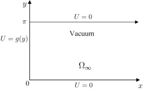
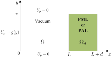
Figure 2.1. Left: schematic diagram of $x$-aligned semi-infinite waveguide. Right: domain reduction by an artificial layer using the PML or PAL technique.

2.1. The PML technique and its error analysis

To solve (2.1) numerically, one commonly-used approach is the PML technique which reduces the semi-infinite strip $\Omega_{\infty}$ in (2.1) to a rectangular domain $\Omega:=(0,L)\times(0,\pi)$ by appending an artificial layer $\Omega_{d}:=(L,L+d)\times(0,\pi)$ with a finite thickness $d$ (see Figure 2.1 (right)). Typically, the artificial layer $\Omega_{d}$ is filled with fictitious absorbing (or lossy) media that can attenuate the waves propagating into the layer. In practice, one would wish the layer can diminish the pollution (due to the reflection) of the original solution in the “physical domain” $\Omega,$ and its thickness $d$ can be as small as possible to save computational cost.

Formally, we solve the reduced Helmholtz equation (called the PML-problem with the PML-solution $U_{\rm p}$) in the finite domain $\Omega\cup\Omega_{d}:$

$$\mathcal{L}_{\rm pml}[U_{\rm p}]:=\Delta_{\rm p}U_{\rm p}+k^{2}n_{\rm p}U_{\rm p}=0\;\;\;{\rm in}\;\;\Omega\cup\Omega_{d};$$ (2.4a)

$$U_{\rm p}(x,0)=U_{\rm p}(x,\pi)=0,\;\;x\in[0,L+d];\;\;$$ (2.4b)

$$U_{\rm p}(0,y)=g(y),\;\;\;U_{\rm p}(L+d,y)=0,\;\;\;y\in[0,\pi],$$ (2.4c)

where we typically impose the homogeneous boundary condition at the outer boundary $x=L+d$ in (2.4c). Note that the operator $\mathcal{L}_{\rm pml}\equiv\mathcal{L}$ in $\Omega,$ while in the PML $\Omega_{d},$ the equation involves variable complex-valued coefficients (in $\Delta_{\rm p}$ and $n_{\rm p}$) derived from complex coordinate stretching as we present shortly. At the interface $x=L,$ we impose the usual transmission conditions (cf. (2.9)).

Remark 2.1.

In practice, it is expected that the error between the solutions of (2.1) and (2.4): $U-U_{\rm p}$ in $\Omega$ (measured in a certain norm) is as small as possible, that is, the “pollution” of the PML is insignificant. Ideally, if $U\equiv U_{\rm p},$ then the layer is non-reflecting. ∎

The critical issue is to construct the governing equation in $\Omega_{d}.$ It is known that the PML-equation can be obtained from the Helmholtz equation: $(\Delta+k^{2})U=0$ in $(\tilde{x},\tilde{y})$-coordinates through the complex coordinate stretching (see, e.g., [16, 43]). More precisely, we introduce the complex coordinate transformation of the form:

$$\begin{cases}\tilde{x}=S(x),\quad\tilde{y}=y,\quad\forall\,(x,y)\in\Omega\cup\Omega_{d}\quad\text{such that}\\[3.0pt] S(x)=x,\;\;\;\forall\,x\in(0,L);\quad\Re\{S^{\prime}(x)\}>0,\ \Im\{S^{\prime}(x)\}>0,\;\;\;\forall\,x\in(L,L+d),\end{cases}$$ (2.5)

where $S(x)$ is a differentiable complex-valued function. One typically chooses

$$S(x)=x+\frac{{\rm i}}{k}\displaystyle\int_{0}^{x}\sigma(t)\,{\rm d}t,\;\;\;\forall\,x\in(0,L+d),$$ (2.6)

where $\sigma(\cdot)\geq 0$ is known as the absorbing function (ABF). Then the substitution

$$\frac{\partial}{\partial x}\to\frac{\partial}{\partial\tilde{x}}=\frac{dx}{d\tilde{x}}\frac{\partial}{\partial x}=\frac{1}{S^{\prime}(x)}\frac{\partial}{\partial x},$$ (2.7)

leads to the PML-equation (cf. [43, (5)]):

$$\frac{\partial}{\partial x}\Big{(}\frac{1}{S^{\prime}(x)}\frac{\partial U_{\rm p}}{\partial x}\Big{)}+\frac{\partial}{\partial y}\Big{(}S^{\prime}(x)\frac{\partial U_{\rm p}}{\partial y}\Big{)}+k^{2}S^{\prime}(x)U_{\rm p}=0,\quad\forall\,(x,y)\in\Omega\cup\Omega_{d},$$ (2.8)

which is supplemented with the transmission conditions at the interface $x=L$:

$$U_{\rm p}\big{|}_{\Omega}=U_{\rm p}\big{|}_{\Omega_{d}},\quad\frac{\partial U_{\rm p}}{\partial x}\Big{|}_{\Omega}=\frac{1}{S^{\prime}(x)}\frac{\partial U_{\rm p}}{\partial x}\Big{|}_{\Omega_{d}},$$ (2.9)

together with the boundary conditions:

$$\begin{split}&U_{\rm p}(x,0)=U_{\rm p}(x,\pi)=0,\;\;\;\;x\in(0,L+d);\quad\\ &U_{\rm p}(0,y)=g(y),\;\;\;\;U_{\rm p}(L+d,y)=0,\;\;\;\;y\in(0,\pi).\end{split}$$ (2.10)

It is noteworthy that with a suitable choice of the ABF $\sigma(t),$ the PML-solution decays sufficiently fast in the artificial layer, so the homogeneous Dirichlet boundary condition is usually imposed at $x=L+d.$

Singer and Turkel [43] conducted error analysis of the PML with usual bounded ABFs. Here, we provide a much more precise description of the error between the original solution $U$ and the PML-solution $U_{\rm p}$ in the physical domain $\Omega$.

Theorem 2.1.

Let $U$ be the solution of (2.1) given by (2.3), and let $U_{\rm p}$ be the PML-solution of (2.8)-(2.10). If $k>0$ is not an integer, then for any $(x,y)\in\Omega,$

$$U(x,y)=U_{\rm p}(x,y)+\sum_{l=1}^{\infty}\hat{g}_{l}\,R_{l}(x)\,e^{{\rm i}\hat{k}_{l}x}\sin(ly),\quad R_{l}(x):=\frac{1-e^{-2{\rm i}\hat{k}_{l}x}}{1-e^{-2{\rm i}\hat{k}_{l}S_{d}}}.$$ (2.11)

If $k>0$ is an integer, then $R_{l}(x)$ for the mode $l=k$ in (2.11) should be replaced by

$$R_{l}(x)=-\frac{S(x)}{S_{d}},\quad\forall\,x\in(0,L).$$ (2.12)

Moreover, we have the following bounds:

• for $0\leq l<k,$

  $$\frac{2|\sin(\hat{k}_{l}x)|}{e^{2\hat{k}_{l}\Im\{S_{d}\}}+1}\leq|R_{l}(x)|\leq\frac{2|\sin(\hat{k}_{l}x)|}{e^{2\hat{k}_{l}{\Im}\{S_{d}\}}-1},\quad\forall\,x\in(0,L);$$ (2.13)

• for $l>k,$

  $$\frac{e^{2|\hat{k}_{l}|x}-1}{e^{2|\hat{k}_{l}|{\Re}\{S_{d}\}}+1}\leq|R_{l}(x)|\leq\frac{e^{2|\hat{k}_{l}|x}-1}{e^{2|\hat{k}_{l}|{\Re}\{S_{d}\}}-1},\quad\forall\,x\in(0,L).$$ (2.14)

In the above, $\hat{k}_{l}:=\sqrt{k^{2}-l^{2}},\,S_{d}:=S(L+d)$ and $S(x)$ is given by (2.5)-(2.6).

To avoid distraction from the main results, we sketch the proof in Appendix A. We see that for fixed $k,l,$ the decay rate of $R_{l}(x)$ is completely determined by the values of ${\Re}\{S_{d}\}$ and ${\Im}\{S_{d}\},$ i.e., the choice of ABF $\sigma(t).$ We now apply Theorem 2.1 to access the performance of PML with some typical ABFs:

$$\text{PML}_{n}:\qquad\sigma(x)=\begin{cases}0,\quad&{\rm if}\;\;x\in(0,L),\\[4.0pt] \sigma_{0}\Big{(}\dfrac{x-L}{d}\Big{)}^{n},\quad&{\rm if}\;\;x\in(L,L+d),\end{cases}$$ (2.15)

and

$$\text{PML}_{\infty}:\qquad\sigma(x)=\begin{cases}0,\quad&{\rm if}\;\;x\in(0,L),\\[4.0pt] \dfrac{\sigma_{0}\,d}{L+d-x},\;\;\;&{\rm if}\;\;x\in(L,L+d),\end{cases}$$ (2.16)

where $\sigma_{0}>0$ is a tuneable constant. We remark that $\text{PML}_{n}$ with integer $n\geq 0,$ is commonly-used (see, e.g., [16, 43, 10]), while $\text{PML}_{\infty}$ was first introduced by Bermúdez et al. [7, 8] (which was advocated for its being “optimal”, “exact” and “parameter-free” in various settings (cf. [7, 8, 39, 37, 15])). It is clear that in $\Omega_{d}$, we have

$$\text{PML}_{n}:\;\;\;S(x)=x+\frac{{\rm i}}{k}\dfrac{d\,\sigma_{0}}{n+1}\Big{(}\dfrac{x-L}{d}\Big{)}^{n+1},\quad{\Re}\{S_{d}\}=L+d,\quad{\Im}\{S_{d}\}=\frac{\sigma_{0}\,d}{(n+1)k},$$ (2.17)

and

$$\text{PML}_{\infty}:\;\;\;S(x)=x+\frac{{\rm i}\,d\,\sigma_{0}}{k}\ln\Big{(}\dfrac{d}{L+d-x}\Big{)},\quad{\Re}\{S_{d}\}=L+d,\quad{\Im}\{S_{d}\}\to\infty.$$ (2.18)

Observe that in both cases, ${\Re}\{S_{d}\}$ does not depend on the choice of ABF $\sigma(t)$. Consequently, the errors corresponding to the evanescent wave components (i.e., $l>k$) behave like

$$|R_{l}(x)|\sim e^{-2\sqrt{l^{2}-k^{2}}(L+d-x)},\quad\forall\,x\in(0,L),$$ (2.19)

so the only possibility to reduce the error is to increase the width $d.$

For the oscillatory wave components (i.e., $l<k$), the PML_∞ can make the error vanish (note: $R_{l}(x)=0$), but for the PML${}_{n},$

$$|R_{l}(x)|\sim 2\big{|}\sin\big{(}\sqrt{k^{2}-l^{2}}x\big{)}\big{|}e^{-2\sqrt{k^{2}-l^{2}}{\sigma_{0}\,d}/{((n+1)k)}},\;\;\;\forall\,x\in(0,L),$$ (2.20)

so one has to enlarge the thickness $d$ of the layer or choose large $\sigma_{0}\,d$ to reduce the error.

As an illustrative example, we consider the exact solution (2.1) with $\{\hat{g}_{l}={\rm i}^{l}J_{l}(k)\}$ (in order to mimic the plane wave expansion):

$$U(x,y)=\sum_{l=1}^{\infty}{\rm i}^{l}J_{l}(k)e^{{\rm i}\sqrt{k^{2}-l^{2}}x}\sin(ly),$$ (2.21)

where $J_{l}(\cdot)$ is the Bessel function. Define the error function:

$${\mathcal{E}}_{\rm p}(x,y)=U(x,y)-U_{\rm p}(x,y)=\sum_{l=1}^{\infty}{\rm i}^{l}J_{l}(k)\,R_{l}(x)\,e^{{\rm i}\sqrt{k^{2}-l^{2}}x}\sin(ly),\quad\forall\,(x,y)\in\Omega.$$ (2.22)

Here, we take $k=9.99,L=1,d=0.1,$ and truncate the infinite series for $l\leq 100$ so that the truncation error is negligible. The error curves $|{\mathcal{E}}_{\rm p}(x,y)|$ with fixed $x=L/2,L$ and $y\in(0,\pi)$ in Figure 2.2 with PML₂ and PML_∞ in (2.15)-(2.16).

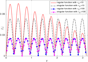
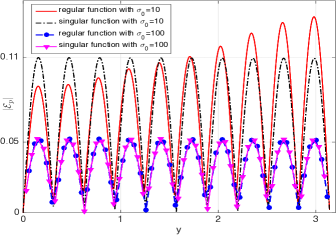
Figure 2.2. Profiles of the error function $|\mathcal{E}_{p}(x,y)|$ of the solution (2.21) with $k=9.99,L=1,d=0.1,$ and $\sigma_{0}/k=10,100$ using PML₂ and PML_∞. Left: the error curve $|\mathcal{E}_{p}(L/2,y)|$ for $y\in(0,\pi).$ Right: the error curve: $|\mathcal{E}_{p}(L,y)|$ for $y\in(0,\pi).$

Observe from Figure 2.2 that the errors of the PML₂ become slightly smaller as $\sigma_{0}$ increases, but they are still large. The PML_∞ using unbounded absorbing functions performs relatively better, but does not significantly improve the classical PML.

Remark 2.2.

The recent work [52] introduced the few-mode DtN technique to deal with the evanescent wave components, while the other modes were treated with the classical PML_n.

Remark 2.3.

As shown in [7], the PML_∞ can completely damp the planar waves of the form: $e^{{\rm i}k_{x}x+{\rm i}k_{y}y}$ with $k_{x}=k\cos\theta_{0},k_{y}=k\sin\theta_{0},$ where $\theta_{0}$ is the incident angle at the left boundary $x=0$ of the half-plane waveguide: $\Delta u+k^{2}u=0,\;x>0,\;-\infty<y<\infty.$ We also refer to [15] for some other successful scenarios. However, it fails to be “exact” and “optimal” in this setting.

Remark 2.4.

Note from (2.18) that for the PML${}_{\infty},$ $S^{\prime}(x)=1+{\rm i}\,\sigma(x)/k\to\infty$ as $x\to L+d,$ so the coefficients in (2.8) are singular at the outer boundary $x=L+d.$ In [7, 8], the use of e.g, Gauss quadrature to avoid sampling the unbounded endpoints was suggested for evaluating the matrices of the linear system in finite-element discretisation. However, for large wavenumber $k$ and very thin layer, much care is needed to deal with the singularity to achieve high order. Moreover, in more complex situations, e.g., the circular/spherical PML, $S(x)$ also appears in the PML-equation, so the logarithmic singularity poses even more challenge in numerical discretisation.

2.2. New PAL technique and its error analysis

As reported in [47], the new PAL was inspired by the design of the “inside-out” invisibility cloak (cf. [51]) using the notion of transformation optics (cf. [36]). In [51], the real rational transformation was introduced to construct the media and design the clocking layer:

$$\rho=\rho(x)=L+\frac{d(x-L)}{L+d-x},\quad\,x\in(L,L+d),\;\;\;\rho\in(L,\infty),$$ (2.23)

which compresses the outgoing waves in the infinite strip: $\rho>L$ into the finite layer: $(L,L+d).$ However, it is known that any attempt of using a real compression coordinate transform fails to work for Helmholtz and Maxwell’s equations. Indeed, according to [32], “any real coordinate mapping from an infinite to a finite domain will result in solutions that oscillate infinitely fast as the boundary is approached – such fast oscillations cannot be represented by any finite-resolution grid, and will instead effectively form a reflecting hard wall.”

To break the curse of infinite oscillation, we propose the complex compression coordinate transformation (C³T), that is, $S(x)=x$ for $x\in(0,L),$ and

$$S(x)=S_{R}(x)+{{\rm i}}\,S_{I}(x),\;\;\;\;x\in(L,L+d),$$ (2.24)

where the real part: $S_{R}(x)=\sigma_{1}\rho(x)$ and the imaginary part: $S_{I}(x)=\sigma_{0}(\rho(x)-L)/k.$ Like (2.16), the imaginary part $S_{I}(x)$ involves an unbounded ABF:

$$S_{I}(x)=\frac{1}{k}\int_{L}^{x}\sigma(t)\,{\rm d}t,\quad\sigma(x)=\sigma_{0}\,\Big{(}\frac{d}{L+d-x}\Big{)}^{2},\quad x\in(L,L+d).$$ (2.25)

For clarity, we denote the PAL-solution by $U_{\rm a}.$ Thanks to (2.7), we obtain the PAL-equation as the counterpart of (2.8)-(2.10):

$$\begin{split}&\frac{\partial}{\partial x}\Big{(}\frac{1}{S^{\prime}(x)}\frac{\partial U_{\rm a}}{\partial x}\Big{)}+\frac{\partial}{\partial y}\Big{(}S^{\prime}(x)\frac{\partial U_{\rm a}}{\partial y}\Big{)}+k^{2}S^{\prime}(x)U_{\rm a}=0,\quad(x,y)\in\Omega\cup\Omega_{d},\\[4.0pt] &U_{\rm a}\big{|}_{\Omega}=U_{\rm a}\big{|}_{\Omega_{d}},\quad\frac{\partial U_{\rm a}}{\partial x}\Big{|}_{\Omega}=\frac{1}{S^{\prime}(x)}\frac{\partial U_{\rm a}}{\partial x}\Big{|}_{\Omega_{d}}\quad{\rm at}\;\;\;x=L,\\[4.0pt] &U_{\rm a}(x,0)=U_{\rm a}(x,\pi)=0;\quad U_{\rm a}(0,y)=g(y),\;\;U_{\rm a}(L+d,y)=0.\end{split}$$ (2.26)

Importantly, we can show that the new PAL is truly exact and non-reflecting.

Theorem 2.2.

Let $U$ be the solution of (2.1), and $U_{\rm a}$ be the solution of (2.26). Then we have

$$U_{\rm a}(x,y)\equiv U(x,y),\quad\forall\,(x,y)\in\Omega.$$ (2.27)

Proof.

Note that the error formula in Theorem 2.1 is valid for general $S(x)$. It is evident that by (2.24), we have ${\Re}\{S(L+d)\}=\infty$ and ${\Im}\{S(L+d)\}=\infty.$ Thus, it follows immediately from (2.13)-(2.14) that $R_{l}(x)=0$ uniformly for all $l$ and $x\in(0,L),$ which implies $U_{\rm a}(x,y)\equiv U(x,y)$ in $\Omega.$ ∎

Different from PML, the truncation by the new PAL is exact at continuous level, but the compression coordinate transformation induces singular coefficients at $x=L+d$ in the PAL-equation (2.26), which causes some numerical difficulties in discretization. To overcome this, we introduce the substitution of the unknown:

$$U_{\rm a}(x,y)=w(x)V_{\rm a}(x,y),\quad w(x)=\dfrac{L+d-x}{d},\;\;\;x\in(L,L+d),$$ (2.28)

with $w(x)=1$ for $x\in(0,L).$ In fact, the transformed PAL-equation in the new unknown $V_{a}$ is free of singularity. To show this, it’s more convenient to work with the variational form. Denote

$${\mathbb{U}}:=\big{\{}u=wv:v\in H^{1}(\Omega\cup\Omega_{d}),\;v(x,0)=v(x,\pi)=0,\;\;x\in(0,L+d)\big{\}},$$

and introduce the sesquilinear form on ${\mathbb{U}}\times{\mathbb{U}}$:

$${\mathcal{B}}(U_{\rm a},\varPsi)=(\boldsymbol{C}\,\nabla U_{\rm a},\nabla\varPsi)-k^{2}(S^{\prime}\,U_{\rm a},\varPsi),$$ (2.29)

where $\boldsymbol{C}={\rm diag}(1/S^{\prime}(x),S^{\prime}(x)),$ and $(\cdot,\cdot)$ is the inner product of $L^{2}(\Omega\cup\Omega_{d}).$

In view of (2.25), a direct calculation leads to $w^{2}(x)S^{\prime}(x)=\alpha=\sigma_{1}+{\rm i}\sigma_{0}/k.$ Then, substituting $U_{\rm a}=wV_{\rm a}$ and $\varPsi=w\varPhi$ into (2.29), we obtain from direct calculation that

$$\begin{split}\widetilde{\mathcal{B}}_{{}_{\Omega_{d}}}(V_{\rm a},\varPhi)={\mathcal{B}}_{{}_{\Omega_{d}}}(wV_{\rm a},w\varPhi)=(\widetilde{\boldsymbol{C}}\,\widetilde{\nabla}V_{\rm a},\widetilde{\nabla}\varPhi)_{\Omega_{d}}-\alpha k^{2}(V_{\rm a},\varPhi)_{\Omega_{d}},\end{split}$$ (2.30)

where $(\cdot,\cdot)_{\Omega_{d}}$ is the inner product on the artificial layer $\Omega_{d},$ and

$$\widetilde{\boldsymbol{C}}={\rm diag}\big{(}w^{2}(x)/\alpha,\;\alpha\big{)},\quad\widetilde{\nabla}=\big{(}w(x)\partial_{x}-1/d,w(x)\partial_{y}\big{)}.$$ (2.31)

It is seen that the substitution can absorb the singular coefficients. In the implementation, one can easily incorporate the substitution into the basis functions and directly approximate $U_{\rm a}$.

Figure 2.3. Profiles of the PML-solution $U_{\rm p}$ with PML₂ in (2.15) and PML_∞ in (2.16) versus PAL solution $U_{a}$ in $\Omega$ and $V_{a}$ in $\Omega_{d}$ with $k=99.99,$ $L=1$ and $d=0.2$ along the $x$-axis at $y=\pi/2$. Left: real part of the solution; Right: imaginary part of the solution. Here, $\sigma_{0}=1.$

In Figure 2.3, we plot the profiles of the solution (2.21) under the PML transformations and the PAL transformation with or without substitution. From the portion in the layer, we observe that the PAL with substitution has a much better behaviour in the layer.

We conclude this section with some numerical results. Consider (2.1) with $k=29.9$ and the boundary source term is prescribed as $g=\sin(5y)-\sin(30y)$ in (2.1b). The semi-infinite strip $\Omega_{\infty}$ in (2.1) is reduced to a rectangular domain $\Omega:=(0,1)\times(0,\pi)$ by appending the PAL layer $\Omega_{d}:=(1,1+d)\times(0,\pi)$ with a finite thickness $d$. Spectral element method based on the sesquilinear form (2.30) is adopted for computation. Numerical results obtained by PAL ($\sigma_{0}=\sigma_{1}=1$) are also compared with PML technique with bounded and unbounded absorbing functions, i.e., PML_n ($n=1$, $\sigma_{0}=10$) and PML_∞ ($\sigma_{0}=10$) in (3.23)-(3.24), respectively.

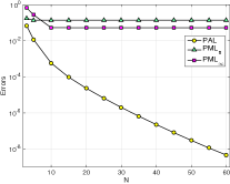
(a) $d=0.1$

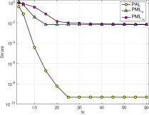
(b) $d=0.5$

Figure 2.4. A comparasion study for waveguide problem: error for PAL, $\text{PML}_{n}$ and $\text{PML}_{\infty}$ against $N$ for $k=29.9$ with different layer thickness (a) $d=0.1$ and (b) $d=0.5$.

In Figure 2.4, we depict the $L^{\infty}$ errors for the numerical solution with these three truncation methods. It can be seen that the errors of the PAL method decreases exponentially to $10^{-10}$ as $N$ increases. However, due to the existence of evanescent modes, the errors saturated at around $10^{-1}$ and $10^{-2}$ for PML method with $d=0.1$ and $d=0.5$, respectively. As analysed previously, the saturation level can only be improved by an increased layer thickness $d$, which is prohibitive due to the increased computational cost.

Test (2.39b) with $\phi=\varpi\psi$ ,we have

$$\begin{split}\big{(}-\mathcal{L}_{\rm pal}[U_{\rm a}],\phi\big{)}_{{\Omega_{d}}}=&\Big{(}\frac{1}{S^{\prime}(x)}\frac{\hat{\partial}V_{a}}{\partial x},\frac{\hat{\partial}\psi}{\partial x}\Big{)}_{{\Omega_{d}}}+\Big{(}\varpi^{2}S^{\prime}(x)\frac{\partial V_{a}}{\partial y},\frac{\partial\psi}{\partial y}\Big{)}_{{\Omega_{d}}}-k^{2}\Big{(}\varpi^{2}S^{\prime}(x)V_{a},\psi\Big{)}_{{\Omega_{d}}}\\ &+\Big{\langle}\frac{1}{S^{\prime}(x)}\frac{\hat{\partial}U_{\rm a}}{\partial x},\phi\Big{\rangle}_{\!\Gamma_{L}}-\Big{\langle}\frac{1}{S^{\prime}(x)}\frac{\hat{\partial}U_{\rm a}}{\partial x},\phi\Big{\rangle}_{\!\Gamma_{d}},\;\;\;{\rm with}\;\;\;\frac{\hat{\partial}}{\partial x}:=\varpi\frac{\partial}{dx}-\frac{1}{d},\end{split}$$ (2.32)

By (2.25)-(LABEL:niceformulas) and (LABEL:substitution1), a direct calculation leads to which shows that the singular coefficients in (2.39b) has been absorbed by the substitution (LABEL:substitution1).

Moreover, we show that the last boundary term in (2.32) vanishes. Actually, this term can be written as

$$\begin{split}\Big{\langle}\frac{1}{S^{\prime}(x)}\frac{\partial U_{\rm a}}{\partial x},\phi\Big{\rangle}_{\!\Gamma_{d}}=&\Big{\langle}\frac{1}{S^{\prime}(x)}\frac{\partial U_{\rm a}}{\partial x}-\sum_{l=1}^{\infty}\frac{2{\rm i}\hat{k}_{l}}{\pi}\Big{(}\int_{0}^{\pi}U_{\rm a}(x,y)\sin(ly)dy\Big{)}\sin(ly),\phi\Big{\rangle}_{\!\Gamma_{d}}\\ &+\varpi^{2}\sum_{l=1}^{\infty}\frac{2{\rm i}\hat{k}_{l}}{\pi}\Big{\langle}\Big{(}\int_{0}^{\pi}V_{\rm a}(x,y)\sin(ly)dy\Big{)}\sin(ly),\psi\Big{\rangle}_{\!\Gamma_{d}}\end{split}$$

Thus, by the transformed outgoing radiation condition (2.42) and the fact that $\varpi(x)\rightarrow 0$ as $x\rightarrow L_{d},$ both the first and the second term vanish in the above equation.

In what follows, we present efficient ideas, based on a suitable substitution, for removing the singularities and diminishing the essential oscillations in the artificial layer so that the outgoing waves can be completely absorbed in the layer. In view of this, we name the integrated approach consisting of the PML with new $S(x)$ and the (unknown) substitution as the PAL.

Instead of solving for $U_{\rm p}$ (denote by $U_{\rm a}$ for PAL to distinguish between existing PMLs), we search for $V_{\rm a}$ in the form:

$$V_{\rm a}(x,y)=\begin{cases}U_{a}(x,y),&{\rm in}\;\;\Omega,\\[4.0pt] {\mathbb{S}}_{w}^{-1}[U_{a}](x,y),&{\rm in}\;\;\Omega_{d},\\ \end{cases}\quad{\rm or}\quad U_{\rm a}(x,y)=\begin{cases}V_{a}(x,y),&{\rm in}\;\;\Omega,\\[4.0pt] {\mathbb{S}}_{w}[V_{a}](x,y),&{\rm in}\;\;\Omega_{d},\\ \end{cases}$$ (2.33)

where, in this setting, ${\mathbb{S}}_{w}$ and its inverse are mappings (for mode-wise substitutions) defined below. Let $w$ be a sequence of functions:

$$w=\big{\{}\hat{w}_{1},\hat{w}_{2},\hat{w}_{3},\cdots\big{\}}\quad{\rm with}\quad\hat{w}_{l}(x)=\frac{L_{d}-x}{d}e^{{\rm i}{\rm Re}\{\hat{k}_{l}(S(x)-L)\}},$$ (2.34)

and let $\{\hat{u}_{a,l}(x)\}$ and $\{\hat{v}_{a,l}(x)\}$ be the expansion coefficients of $U_{\rm a}$ and $V_{\rm a}$ in the sine-series of $\{\sin(ly)\}$, respectively. Then we define

$$U_{\rm a}={\mathbb{S}}_{w}[V_{a}]=\sum_{l=1}^{\infty}\hat{w}_{l}(x)\hat{v}_{a,l}(x)\sin(ly);\quad V_{\rm a}={\mathbb{S}}_{w}^{-1}[U_{a}]=\sum_{l=1}^{\infty}\hat{w}_{l}^{-1}(x)\hat{u}_{a,l}(x)\sin(ly).$$ (2.35)

Test (2.39b) with $\phi=\sum_{l=1}^{\infty}\hat{w}_{l}(x)\hat{\psi}_{l}(x)\sin(ly),$ we have

$$\begin{split}\big{(}-\mathcal{L}_{\rm pal}[U_{\rm a}],\phi\big{)}_{{\Omega_{d}}}=&\frac{\pi}{2}\sum_{i=1}^{\infty}\Big{\{}\Big{(}\frac{|\hat{w}_{l}^{\prime}|^{2}}{S^{\prime}}\hat{\partial}_{x}^{l}\hat{v}_{l},\hat{\partial}_{x}^{l}\hat{\psi}_{l}\Big{)}_{I_{d}}+(l^{2}-k^{2})\big{(}S^{\prime}|\hat{w}_{l}|^{2}\hat{v}_{l},\hat{\psi}_{l}\big{)}_{I_{d}}\Big{\}}\\ &+\Big{\langle}\frac{1}{S^{\prime}}\frac{\partial U_{\rm a}}{\partial x},\phi\Big{\rangle}_{\!\Gamma_{L}}-\Big{\langle}\frac{1}{S^{\prime}}\frac{\partial U_{\rm a}}{\partial x},\phi\Big{\rangle}_{\!\Gamma_{d}},\;\;\;{\rm with}\;\;\;\hat{\partial}_{x}^{l}:=\frac{\hat{w}_{l}}{\hat{w}_{l}^{\prime}}\frac{d}{dx}+1,\end{split}$$ (2.36)

where $\Gamma_{L}$ and $\Gamma_{d}$ are the inner and outer boundary of $\Omega_{d},$ respectively. Denote

$$\alpha:=\sigma_{0}(1+{\rm i}),\quad\varpi:={(L_{d}-x)}/{d}.$$ (2.37)

By (2.25)-(LABEL:niceformulas) and (2.48), a direct calculation leads to

$$\frac{|\hat{w}_{l}^{\prime}|^{2}}{S^{\prime}}=\frac{1}{\alpha}\big{(}\sigma_{0}^{2}|\hat{k}_{l}|^{2}+d^{-2}\varpi^{2}\big{)},\;\;\;S^{\prime}|\hat{w}_{l}|^{2}=\alpha,\;\;\;\frac{\hat{w}_{l}}{\hat{w}_{l}^{\prime}}=\frac{d\varpi^{2}}{-\varpi\pm{\rm i}\sigma_{0}|\hat{k}_{l}|d},$$ (2.38)

where the notation $\pm$ in the last term of (2.51) takes “plus” when $k>l$ ( “minus” when $k<l$).

Moreover, we show that the last boundary term in (2.49) vanishes. Actually, this term can be written as

$$\Big{\langle}\frac{1}{S^{\prime}}\frac{\partial U_{\rm a}}{\partial x},\phi\Big{\rangle}_{\!\Gamma_{d}}=\Big{\langle}\frac{1}{S^{\prime}}\frac{\partial U_{\rm a}}{\partial x}-\sum_{l=1}^{\infty}\frac{2{\rm i}\hat{k}_{l}}{\pi}\Big{(}\int_{0}^{\pi}U_{\rm a}(x,y)\sin(ly)dy\Big{)}\sin(ly),\phi\Big{\rangle}_{\!\Gamma_{d}}+\frac{{\rm i}\pi}{2}\varpi^{2}\sum_{l=1}^{\infty}\hat{k}_{l}\hat{v}_{l}(x)\overline{\hat{\psi}_{l}}(x)\big{|}_{x=L_{d}}.$$

Thus, by the transformed outgoing radiation condition (2.42) and the fact that $\varpi(x)\rightarrow 0$ as $x\rightarrow L_{d},$ both the first and the second term vanish in the above equation.

Remark 2.5.

It is very important to observe that

• Compared with (2.39b), the singular coefficient $S^{\prime}(x)$ has been absorbed by the substitution (2.48) and the involved coefficients in (2.49) become regular.

• The strongly indefiniteness due to $(l^{2}-k^{2})S^{\prime}(x)$ in (2.39b) has been reduced to $(l^{2}-k^{2})\alpha$ in (2.49). In fact, $\hat{w}_{l}$ incorporates complex exponential to capture the oscillation of $U_{\rm a}$. By (2.46) and (2.48), $\hat{v}_{l}(x)$ is expected to behave like $e^{-\sigma_{0}|\hat{k}_{l}|(x-L)/(L_{d}-x)}/(L_{d}-x),$ which decays smoothly to $0$ as $x\rightarrow L_{d}$ and has no oscillation at all.

• The outgoing boundary condition is transformed to the outer boundary layer $\Omega_{d}$, this naturally eliminate the last boundary term in (2.49).

the essential idea to introduce the (componentwise) substitution, that is, we solve for

More insights about the choice!

From the general setting in (2.5)-(2.7), the PAL-equation in $\Omega_{d}$ takes the same form as (2.8). As with (LABEL:UPML), the coefficients become singular at the outer boundary, since $S_{I}^{\prime}(x),S_{R}^{\prime}(x)$ tend to infinity as $x\to L_{d}.$ We summarise the PAL-equation, together with the idea of resolving the singularities, as follows

$$\mathcal{L}_{\rm pal}[U_{\rm a}]:=\Delta U_{\rm a}+k^{2}U_{\rm a}=0\;\;\;{\rm in}\;\;\Omega;$$ (2.39a)

$$\mathcal{L}_{\rm pal}[U_{\rm a}]:=\frac{\partial}{\partial x}\Big{(}\frac{1}{S^{\prime}(x)}\frac{\partial U_{\rm a}}{\partial x}\Big{)}+\frac{\partial}{\partial y}\Big{(}S^{\prime}(x)\frac{\partial U_{\rm a}}{\partial y}\Big{)}+k^{2}S^{\prime}(x)U_{\rm a}=0\;\;\;{\rm in}\;\;\Omega_{d};$$ (2.39b)

$$U_{\rm a}\big{|}_{\Omega}=U_{\rm a}\big{|}_{\Omega_{d}},\quad\frac{\partial U_{\rm a}}{\partial x}\Big{|}_{\Omega}=\frac{1}{S^{\prime}(x)}\frac{\partial U_{\rm a}}{\partial x}\Big{|}_{\Omega_{d}},\quad{\rm at}\;\;x=L,$$ (2.39c)

$$U_{\rm a}(x,0)=U_{\rm a}(x,\pi)=0,\;\;x\in[0,L+d];\;\;U_{\rm a}(0,y)=g(y),\;\;y\in[0,\pi];$$ (2.39d)

where we transform the radiation condition (2.2) from the far field to the outer boundary $x=L_{d}:$

$$\frac{1}{S^{\prime}(x)}\frac{\partial U_{\rm a}}{\partial x}-\sum_{l=1}^{\infty}\frac{2{\rm i}\hat{k}_{l}}{\pi}\Big{(}\int_{0}^{\pi}U_{\rm a}(x,y)\sin(ly)dy\Big{)}\sin(ly)=0.$$ (2.40)

To deal with the singular coefficients, we make a substitution, and formally, set

$$U_{\rm a}={\mathbb{S}}_{\boldsymbol{w}}[V_{a}]=\sum_{l=1}^{\infty}w_{l}(x)\hat{V}_{l}(x)\sin(ly),\quad w_{l}(x)=\frac{L_{d}-x}{d}e^{{\rm i}{\rm Re}\{\hat{k}_{l}(S(x)-L)\}}$$ (2.41)

and $V_{a}$ is a well-behaved function with

$$V_{a}(x,y)=\sum_{l=1}^{\infty}\hat{V}_{l}(x)\sin(ly),\quad\hat{V}_{l}(x)=\frac{2}{\pi}\int_{0}^{\pi}V_{a}(x,y)\sin(ly)dy.$$

We can derive the governing equation

$$\frac{1}{S^{\prime}(x)}\frac{\partial U_{\rm a}}{\partial x}=\sum_{l=1}^{\infty}{{\rm i}\hat{k}}\,\hat{c}_{l}\,e^{{\rm i}\hat{k}_{l}S(x)}\sin(ly)=\sum_{l=1}^{\infty}\frac{2{\rm i}\hat{k}_{l}}{\pi}\Big{(}\int_{0}^{\pi}U_{\rm a}(x,y)\sin(ly)dy\Big{)}\sin(ly),\;\;\;{\rm in}\;\;\Omega_{d},$$ (2.42)

where

$$\hat{c}_{l}=\frac{2}{\pi}e^{-{\rm i}\hat{k}_{l}L}\Big{(}\int_{0}^{\pi}U_{\rm a}(L,y)\sin(ly)dy\Big{)}.$$

Different from the PML-problem (2.4), the PAL-problem (2.39) has no “pollution” at all. Thus the PAL layer is totally non-reflecting in $\Omega_{d}.$

Theorem 2.3.

The solutions $U$ and $U_{\rm a}$ for the original problem (2.1) and the PAL problem (2.39) are identical, i.e., $U\equiv U_{\rm a}$ in $\Omega.$

Proof.

The scattering problem (2.1) is equivalent to the following formulation (cf. [27]):

$$\mathcal{L}[U]=0\;\;\;{\rm in}\;\;\;\Omega;\quad\frac{\partial U}{\partial x}-\mathcal{T}[U]=0\;\;{\rm at}\;\;x=L;$$ (2.43a)

$$U(x,0)=U(x,\pi)=0,\;\;x\in[0,L];\;\;\;U(0,y)=g(y),\;\;\;y\in[0,\pi],$$ (2.43b)

where the Dirichlet-to-Neumann operator $\mathcal{T}$ is defined by

$$\mathcal{T}[U]:=\sum_{l=1}^{\infty}\frac{2{\rm i}\hat{k}_{l}}{\pi}\Big{(}\int_{0}^{\pi}U(L,y)\sin(ly)dy\Big{)}\sin(ly).$$ (2.44)

Consider the PAL-problem in $\Omega_{d}:$

$$\mathcal{L}_{\rm pal}[U_{\rm a}]=0\;\;{\rm in}\;\;\Omega_{d};\;\;U_{\rm a}(x,0)=U_{\rm a}(x,\pi)=0,\;\;x\in[L,L_{d}];\;\;U_{\rm a}(L,y)=\Psi(y),\;\;\;y\in[0,\pi],$$ (2.45)

where $\Psi(y)$ is passed from the interior solution $U_{\rm a}|_{\Omega}$ of (2.39) at $x=L$ and $U_{\rm a}$ satisfies the transformed outgoing boundary condition (2.42). By Fourier expansion method, we obtain that

$$U_{\rm a}=\sum_{l=1}^{\infty}\hat{\Psi}_{l}e^{{\rm i}\hat{k}_{l}(S(x)-L)}\sin(ly),\quad{\rm with}\;\;\;\hat{\Psi}_{l}=\frac{2}{\pi}\int_{0}^{\pi}\Psi(y)\sin(ly)dy.$$ (2.46)

A direct partial differentiation of the above solution with respect to $x$ leads to

$$\frac{\partial U_{\rm a}}{\partial x}=S^{\prime}(x)\sum_{l=1}^{\infty}{\rm i}\hat{k}_{l}\hat{\Psi}_{l}e^{{\rm i}\hat{k}_{l}(S(x)-L)}\sin(ly).$$

Note from (2.25) that $S(L)=L,$ and the continuity relation (2.39c), we have that

$$\frac{\partial U_{\rm a}}{\partial x}\Big{|}_{\Omega_{d}}=S^{\prime}(L)\sum_{l=1}^{\infty}{\rm i}\hat{k}_{l}\hat{\Psi}_{l}\sin(ly)=S^{\prime}(L)\frac{\partial U_{\rm a}}{\partial x}\Big{|}_{\Omega}\;\;\;{\rm at}\;\;x=L,$$

which, together with (2.55) leads to

$$\frac{\partial U_{\rm a}}{\partial x}\Big{|}_{\Omega}-\mathcal{T}[U_{\rm a}|_{\Omega}]=0\;\;{\rm at}\;\;x=L.$$ (2.47)

We observe that the interior PAL-problem (2.39a) $+$ the boundary condition (2.47) is identical with (2.43). This ends the proof. ∎

To deal with the singular coefficients, we make a substitution, and formally, set

$$U_{\rm a}={\mathbb{S}}_{w}[V_{a}]=\sum_{l=1}^{\infty}\hat{w}_{l}(x)\hat{v}_{l}(x)\sin(ly),\quad\hat{w}_{l}(x)=\frac{L_{d}-x}{d}e^{{\rm i}{\rm Re}\{\hat{k}_{l}(S(x)-L)\}},$$ (2.48)

and $\{\hat{v}_{l}(x)\}_{l=1}^{\infty}$ are the Fourier sine series of $V_{a}$,

$$V_{a}(x,y)=\sum_{l=1}^{\infty}\hat{v}_{l}(x)\sin(ly),\quad\hat{v}_{l}(x)=\frac{2}{\pi}\int_{0}^{\pi}V_{a}(x,y)\sin(ly)dy.$$

Test (2.39b) with $\phi=\sum_{l=1}^{\infty}\hat{w}_{l}(x)\hat{\psi}_{l}(x)\sin(ly),$ we have

$$\begin{split}\big{(}-\mathcal{L}_{\rm pal}[U_{\rm a}],\phi\big{)}_{{\Omega_{d}}}=&\frac{\pi}{2}\sum_{i=1}^{\infty}\Big{\{}\Big{(}\frac{|\hat{w}_{l}^{\prime}|^{2}}{S^{\prime}}\hat{\partial}_{x}^{l}\hat{v}_{l},\hat{\partial}_{x}^{l}\hat{\psi}_{l}\Big{)}_{I_{d}}+(l^{2}-k^{2})\big{(}S^{\prime}|\hat{w}_{l}|^{2}\hat{v}_{l},\hat{\psi}_{l}\big{)}_{I_{d}}\Big{\}}\\ &+\Big{\langle}\frac{1}{S^{\prime}}\frac{\partial U_{\rm a}}{\partial x},\phi\Big{\rangle}_{\!\Gamma_{L}}-\Big{\langle}\frac{1}{S^{\prime}}\frac{\partial U_{\rm a}}{\partial x},\phi\Big{\rangle}_{\!\Gamma_{d}},\;\;\;{\rm with}\;\;\;\hat{\partial}_{x}^{l}:=\frac{\hat{w}_{l}}{\hat{w}_{l}^{\prime}}\frac{d}{dx}+1,\end{split}$$ (2.49)

where $\Gamma_{L}$ and $\Gamma_{d}$ are the inner and outer boundary of $\Omega_{d},$ respectively. Denote

$$\alpha:=\sigma_{0}(1+{\rm i}),\quad\varpi:={(L_{d}-x)}/{d}.$$ (2.50)

By (2.25)-(LABEL:niceformulas) and (2.48), a direct calculation leads to

$$\frac{|\hat{w}_{l}^{\prime}|^{2}}{S^{\prime}}=\frac{1}{\alpha}\big{(}\sigma_{0}^{2}|\hat{k}_{l}|^{2}+d^{-2}\varpi^{2}\big{)},\;\;\;S^{\prime}|\hat{w}_{l}|^{2}=\alpha,\;\;\;\frac{\hat{w}_{l}}{\hat{w}_{l}^{\prime}}=\frac{d\varpi^{2}}{-\varpi\pm{\rm i}\sigma_{0}|\hat{k}_{l}|d},$$ (2.51)

where the notation $\pm$ in the last term of (2.51) takes “plus” when $k>l$ ( “minus” when $k<l$).

Moreover, we show that the last boundary term in (2.49) vanishes. Actually, this term can be written as

$$\Big{\langle}\frac{1}{S^{\prime}}\frac{\partial U_{\rm a}}{\partial x},\phi\Big{\rangle}_{\!\Gamma_{d}}=\Big{\langle}\frac{1}{S^{\prime}}\frac{\partial U_{\rm a}}{\partial x}-\sum_{l=1}^{\infty}\frac{2{\rm i}\hat{k}_{l}}{\pi}\Big{(}\int_{0}^{\pi}U_{\rm a}(x,y)\sin(ly)dy\Big{)}\sin(ly),\phi\Big{\rangle}_{\!\Gamma_{d}}+\frac{{\rm i}\pi}{2}\varpi^{2}\sum_{l=1}^{\infty}\hat{k}_{l}\hat{v}_{l}(x)\overline{\hat{\psi}_{l}}(x)\big{|}_{x=L_{d}}.$$

Thus, by the transformed outgoing radiation condition (2.42) and the fact that $\varpi(x)\rightarrow 0$ as $x\rightarrow L_{d},$ both the first and the second term vanish in the above equation.

Remark 2.6.

It is very important to observe that

• Compared with (2.39b), the singular coefficient $S^{\prime}(x)$ has been absorbed by the substitution (2.48) and the involved coefficients in (2.49) become regular.

• The strongly indefiniteness due to $(l^{2}-k^{2})S^{\prime}(x)$ in (2.39b) has been reduced to $(l^{2}-k^{2})\alpha$ in (2.49). In fact, $\hat{w}_{l}$ incorporates complex exponential to capture the oscillation of $U_{\rm a}$. By (2.46) and (2.48), $\hat{v}_{l}(x)$ is expected to behave like $e^{-\sigma_{0}|\hat{k}_{l}|(x-L)/(L_{d}-x)}/(L_{d}-x),$ which decays smoothly to $0$ as $x\rightarrow L_{d}$ and has no oscillation at all.

• The outgoing boundary condition is transformed to the outer boundary layer $\Omega_{d}$, this naturally eliminate the last boundary term in (2.49).

2.2.1. Complex compression coordinate transformation

The above observations for the errors of PML techniques motivate us to choose unbounded functions for both $\rho_{{}_{\!R}}(x)$ and $\rho_{{}_{\!I}}(x),$ which leads to the first step of the proposed PAL technique.

Theorem 2.4.

By the complex compression coordinate transformation proposed in [47]

$$\rho_{{}_{\!R}}(x)=L+z(x),\quad\rho_{{}_{\!I}}(x)=z(x),\quad z(x)=\frac{d(x-L)}{L+d-x},\quad x\in(L,L+d),$$ (2.52)

we obtain the expression of the variable coefficient $n(x)$ of the PAL equation in (2.8)

$$n={\alpha}\varpi^{-2},\quad\alpha:=1+{\rm i}\sigma_{0},\;\;\varpi=(L+d-x)/d.$$ (2.53)

The last equation of (LABEL:truncatedpbm) is replaced by the radiation condition that $u_{a}$ is “outgoing” as $x\rightarrow L+d.$ Accordingly, the truncated problem and the original problem (2.1) are equivalent, i.e., we have that $u=u_{f}$ in $\Omega_{f}.$

Proof.

We only need to prove the equivalence for each Fourier mode. The original problem (2.1) for each mode is equivalent to the following formulation (cf. [27]):

$$u_{m}^{\prime\prime}+(k^{2}-m^{2})u_{m}=0,\;\;x\in(0,L),\quad u_{m}(0)=f_{m},\;\;u_{m}^{\prime}-\mathcal{T}_{m}^{k}[u_{m}]=0\;\;{\rm at}\;\;x=L,$$ (2.54)

where the Dirichlet-to-Neumann operator $\mathcal{T}_{m}^{k}[\cdot]$ is defined by

$$\mathcal{T}_{m}^{k}[\phi]:={\rm i}k\phi e^{{\rm i}k_{m}x},\;\;{\rm for}\;\;k>m;\quad\mathcal{T}_{m}^{k}[\phi]:=-k_{m}\phi e^{-k_{m}x}\;\;k<m.$$ (2.55)

Following the proof of Theorem LABEL:PMLsolu, it is straightforward to obtain the solution of the PAL layer

$$u_{m}^{a}(x)=\psi_{m}e^{{\rm i}k_{m}(\rho_{{}_{\!R}}(x)+{\rm i}\sigma_{0}\rho_{{}_{\!I}}(x))},\;\;{\rm for}\;\;k>m;\quad u_{m}^{a}(x)=\psi_{m}e^{-k_{m}(\rho_{{}_{\!R}}(x)+{\rm i}\sigma_{0}\rho_{{}_{\!I}}(x))},\;\;{\rm for}\;\;k<m,$$ (2.56)

where $u_{m}^{a}(L)=\psi_{m}.$ A direct differentiation of the above equation leads to

$$(u_{m}^{a})^{\prime}(x)={\rm i}k_{m}n(x)u_{m}^{a}(x),\;\;{\rm for}\;\;k>m;\quad(u_{m}^{a})^{\prime}(x)=-k_{m}n(x)u_{m}^{a}(x),\;\;{\rm for}\;\;k<m,$$

where $n(x)$ is defined in (2.53). Note that $n(L)=\alpha$ in (2.53). Restricting the above equation at $x=L$ leads to

$$(u_{m}^{a})^{\prime}(L)={\rm i}k_{m}\alpha\psi_{m}e^{{\rm i}k_{m}L},\;\;{\rm for}\;\;k>m;\quad(u_{m}^{a})^{\prime}(L)=-k_{m}\alpha\psi_{m}e^{-k_{m}L},\;\;{\rm for}\;\;k<m.$$

By the above relation and the continuity relation that

$$u_{m}^{f}=u_{m}^{a}=\psi_{m},\;\;(u_{m}^{f})^{\prime}(L)={\alpha}^{-1}(u_{m}^{a})^{\prime}(L),$$

we have that

$$u_{m}^{f}-\mathcal{T}_{m}^{k}[u_{m}^{f}]=0\;\;{\rm at}\;\;x=L.$$

Thus, the truncated problem is equivalent to

$$\big{(}u_{m}^{f}\big{)}^{\prime\prime}+(k^{2}-m^{2})u_{m}^{f}=0,\;x\in(0,L),\;\;u_{m}^{f}(0)=f_{m},\;\;(u_{m}^{f})^{\prime}-\mathcal{T}_{m}^{k}[u_{m}^{f}]=0\;\;{\rm at}\;\;x=L,$$ (2.57)

which is identical with the original problem (2.54). This ends the proof. ∎

Though lack of truncation error, the simulation of the PAL problem is challenging due to (i) the coefficient $n(x)\rightarrow\infty$ as $x\rightarrow L+d$; (ii) the solution (2.56) oscillates infinitely near the outer boundary, as the involvement of the oscillation parts $e^{{\rm i}k_{m}\rho_{{}_{\!R}}(x)}$ and $e^{-{\rm i}k_{m}\sigma_{0}\rho_{{}_{\!I}}(x)}.$ Such a solution cannot be well approximated by standard polynomial basis, which motivates us the second step of PAL technique.

Add numerical illustration to show this point!

2.2.2. Variable substitution

To handle the singularity and remove essential oscillations of $u_{m}^{a}$ in (2.56), we introduce the following substitution in $(L,L+d)$:

$$u_{m}^{a}(x)=v_{m}(x)w_{m}(x),\;\;w_{m}(x)={\varpi(x)}\cdot\begin{cases}e^{{\rm i}k_{m}z(x)},\;\;&k>m,\\ e^{-{\rm i}k_{m}\sigma_{0}z(x)},\;\;&k<m,\end{cases}$$ (2.58)

where $z(x)$ and $\varpi(x)$ are defined in (2.52)-(2.53). It is important to remark that

• We incorporate the complex exponential to capture the oscillation of $u_{m}^{a},$ so that $v_{m}$ essentially has no oscillation for arbitrary high wavenumber and very thin layer.

• In real implementation, we can build in the substitution into the basis functions, and formally approximate $u_{m}^{a}$ by non-conventional basis:

  $${\rm span}\big{\{}\psi_{mj}(x,y)=\phi_{j}(x)w_{m}(x)\,:\,0\leq j\leq N\big{\}},$$ (2.59)

  where $v_{m}$ is essentially approximated by the usual polynomial or piecewise polynomial basis $\{\phi_{j}\}$ in spectral/spectral-element methods.

We find it is more convenient to carry out the substitution through the variational form. Let $L^{2}_{\omega}(I)$ be a weighted space of square integrable functions with the inner product and norm denoted by $(\cdot,\cdot)_{\omega,I}$ and $\|\cdot\|_{\omega,I}$ as usual. Let $I=I_{\!f}\cup I_{a}=(0,L)\cup(L,L+d),$ and assume $f_{m}=0.$

Formally, we define the bilinear form associated with (LABEL:wavetruncate) in $I_{\!f}$ coupled with PAL equation in $I_{a}$ for each Fourier mode:

$$\begin{split}&\mathbb{B}^{m}_{{}_{I}}(u_{m},\phi):=\mathbb{B}^{m}_{{}_{I_{\!f}}}(u_{m},\phi)+\mathbb{B}^{m}_{{}_{I_{a}}}(u_{m},\phi)\;\;{\rm with}\;\;\mathbb{B}^{m}_{{}_{I_{\!f}}}(u_{m},\phi)=(u_{m}^{\prime},\phi^{\prime})_{{}_{I_{\!f}}}-(k^{2}-m^{2})(u_{m},\phi)_{{}_{I_{\!f}}},\\ &\mathbb{B}^{m}_{{}_{I_{a}}}(u_{m},\phi)=\big{(}n^{-1}u_{m}^{\prime},\phi^{\prime}\big{)}_{{}_{I_{a}}}-(k^{2}-m^{2})\big{(}nu_{m},\phi\big{)}_{{}_{I_{a}}}-(n^{-1}u_{m}^{\prime}\bar{\phi})|_{x=L+d}.\end{split}$$ (2.60)

In what follows, we omit the subscript $I_{a}$ when no confusions caused.

Theorem 2.5.

With the substitution $u_{m}=v_{m}w_{m}$ and $\phi=\psi_{m}w_{m}$ in (2.58), when $k>m,$ we have

$$\begin{split}\mathbb{B}^{m}_{{}_{I_{a}}}(u_{m},\phi)&={\alpha}^{-1}\big{(}v_{m}^{\prime},\psi_{m}^{\prime}\big{)}_{\varpi^{4}}+{\alpha}^{-1}\big{(}v_{m}^{\prime},p\psi_{m}\big{)}_{\varpi^{2}}+{\alpha}^{-1}\big{(}pv_{m},\psi_{m}^{\prime}\big{)}_{\varpi^{2}}+\big{(}qv_{m},\psi_{m}\big{)},\\ \end{split}$$ (2.61)

where we recall $\alpha=1+{\rm i}\sigma_{0},$ $\varpi=(L+d-x)/d$, and

$$p=-d^{-1}\varpi+{\rm i}k_{m},\quad q=(\alpha^{-1}-\alpha)k_{m}^{2}+\alpha^{-1}d^{-2}\varpi^{2},\quad {\rm when}\;\;k>m,$$ (2.62a)

$$p=-d^{-1}\varpi+{\rm i}k_{m}\sigma_{0},\quad q=(\sigma_{0}^{2}\alpha^{-1}-\alpha)k_{m}^{2}+\alpha^{-1}d^{-2}\varpi^{2},\quad {\rm when}\;\;k<m.$$ (2.62b)

Proof.

The proof is postponed in Appendix B. ∎

Remark 2.7.

Some remarks are in order.

• Compared with the singular coefficients in (2.53), we observe from (2.62) that the involved coefficients become regular. In particular, $q$ is uniformly bounded above and below away from zero.

• The DtN boundary condition is transformed to the outer boundary $x=L+d,$ this naturally eliminate the boundary term in (2.60).

• When $u_{m}$ is approximated by a non-conventional basis (2.59), we can use (2.61)-(2.62) to compute the matrices of the linear system. In fact, $I_{a}$ can be replaced by any element of a non-overlapping partition of $I_{a}.$ ∎

Notwithstanding its simplicity, the development of the PAL for waveguide problems elaborates all the necessary ingredients and the significant differences of our approach from the PML: (i) we use the compression transformation for both the real and imaginary parts in (LABEL:generaltrans) so we can directly transform the far-field radiation conditions to $x=L+d$ and (ii) more importantly, the substitution (2.58) allows us to remove the singularity and oscillation in the layer leading to well-behaved functions which can be accurately approximated by standard approximation tools.

3. Star-shaped domain truncation and circular PAL

One of the main purposes of this paper is to design the PAL with a general star-shaped domain truncation for solving the two-dimensional time-harmonic acoustic wave scattering problems. More precisely, we consider the exterior domain:

$$\mathscr{L}[U]:=\Delta U+k^{2}U=f\quad{\rm in}\;\;\;\Omega_{e}:=\mathbb{R}^{2}\setminus\bar{D};$$ (3.1a)

$$U=g\;\;\;{\rm on}\;\;\partial D;\qquad\Big{|}\frac{\partial U}{\partial r}-{\rm i}kU\Big{|}\leq\frac{c}{r}\quad{\rm for}\;\;\;r=:|\boldsymbol{x}|\gg 1,$$ (3.1b)

where $D\subset{\mathbb{R}}^{2}$ is a bounded scatterer with Lipschitz boundary $\Gamma_{\!D}=\partial D,$ and $g\in H^{1/2}(\Gamma_{\!D}).$ Here, we assume that the source $f$ is compactly supported in a disk $B(\supset D).$ The far-field condition in (3.1b) is known as the Sommerfeld radiation boundary condition. The PAL technique to be introduced is applicable to the Helmholtz problems with other types of boundary conditions such as Dirichlet or impendence boundary condition on $\Gamma_{\!D},$ and also to solve acoustic wave propagations in inhomogeneous media in bounded domains.

We start with a general set-up for the star-shaped truncated domain, and provide new perspectives of the circular PAL reported in [47], which shed lights on the study of general PAL with star-shaped domain truncation in the forthcoming section.

3.1. Star-shaped truncated domain

As illustrated in Figure 3.1, we enclose $\bar{D}$ by a star-shaped domain $\Omega_{\rm s}$ with respect to the origin. Assume that the boundary of $\Omega_{\rm s}$ is piecewise smooth with the parametric form in the polar coordinates, viz.,

$$\Gamma_{\!R_{1}}:=\partial\Omega_{\rm s}=\big{\{}(r,\theta)\,:\,r=R_{1}(\theta),\;\;\theta\in[0,2\pi)\big{\}},$$ (3.2)

or equivalently, $\Gamma_{\!R_{1}}$ has the parametric form in Cartesian coordinates:

$$\Gamma_{\!R_{1}}=\big{\{}\boldsymbol{x}=(x,y)\,:\,x=R_{1}(\theta)\cos\theta,\;y=R_{1}(\theta)\cos\theta,\;\theta\in[0,2\pi)\big{\}}.$$ (3.3)

Then the artificial layer is formed by surrounding $\Omega_{\rm s}$ with

$$\Omega_{\varrho}^{\rm PAL}:=\big{\{}(r,\theta)\,:\,R_{1}(\theta)<r<R_{2}(\theta):=\varrho R_{1}(\theta),\;\;\theta\in[0,2\pi)\big{\}},$$ (3.4)

where the constant $\varrho>1$ can tune the “thickness” of the layer. The layer $\Omega_{\varrho}^{\rm PAL}$ provides a star-shaped domain truncation of the unbounded domain $\Omega_{e}$. We further denote the domain of interest and the real computational domain, respectively, by

$$\Omega:=\Omega_{\rm s}\setminus\bar{D},\quad\Omega_{\rm c}:=\Omega_{\varrho}^{\rm PAL}\cup\Omega\cup\Gamma_{\!R_{1}},$$ (3.5)

where we need to approximation the original solution in $\Omega,$ but have to couple the original equation in $\Omega$ with the artificial equation in $\Omega_{\varrho}^{\rm PAL}$ in real computation.

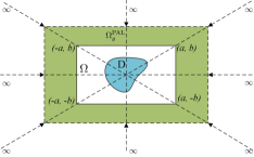
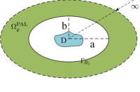
Figure 3.1. Schematic illustration of the rectangular PAL with four trapezoidal patches (left), the elliptical PAL (right), and the compression transformation from radial direction.

Since the choice of the truncated domains is a prior arbitrary, it could be an advantageous to choose non-classical shapes to offer more flexibility to deal with non-standard geometry of the scatterer and inhomogeneity of the media. It is important to note that the configuration of the artificial layer is solely determined by the parametric form of $R_{1}(\theta)$ and the tuning “thickness” parameter $\varrho.$ We list below some typical examples of such star-shaped domain truncation.

• In the circular case, the artificial layer is an annulus, i.e.,

  $$\Omega_{\varrho}^{\rm PAL}=\{R_{1}<r<R_{2}=\varrho R_{1},\;0\leq\theta<2\pi\},$$ (3.6)

  where $R_{1}$ is independent of $\theta.$ As a variant, the “perturbed” annular layer takes the form:

  $$\Omega_{\varrho}^{\rm PAL}=\{R_{1}(\theta)=a+b\sin\theta<r<R_{2}(\theta)=\varrho R_{1}(\theta),\;0\leq\theta<2\pi\},$$ (3.7)

  where $a,b>0$ are some given constants.

• In the rectangular case, we take for instance the boundary $\Gamma_{\!R_{1}}$ as a square with four vertices: $(a,b),(-a,b),(-a,-b),$ $(a,-b)$ with $a,b>0$ (see Figure 3.1 (left)). Then we have

  $$R_{1}(\theta)=\begin{cases}a\sec\theta,\quad&\theta\in[0,\theta_{0})\cup[2\pi-\theta_{0},2\pi),\\[2.0pt] b\csc\theta,\quad&\theta\in[\theta_{0},\pi-\theta_{0}),\\[2.0pt] -a\sec\theta,\quad&\theta\in[\pi-\theta_{0},\pi+\theta_{0}),\\[2.0pt] -b\csc\theta,\quad&\theta\in[\pi+\theta_{0},2\pi-\theta_{0}),\end{cases}\qquad\theta_{0}=\arctan\frac{b}{a}.$$ (3.8)

  Similarly, we can consider a general rectangular domain truncation.

• If we choose $\Gamma_{\!R_{1}}$ to be an ellipse: $\frac{x^{2}}{a^{2}}+\frac{y^{2}}{b^{2}}=1$ with $a>b>0$ (see Figure 3.1 (right)), then we have

  $$R_{1}(\theta)=\frac{ab}{\sqrt{b^{2}+(a^{2}-b^{2})\sin^{2}\theta}},\quad\theta\in[0,2\pi).$$ (3.9)

Now, the key issue is how to construct the governing equation in the artificial layer. In practice, one wishes (i) the solution of the resulted coupled problem in $\Omega_{\rm c}$ can approximate the original solution $U|_{\Omega}$ as accurate as possible to avoid the pollution of the truncation, but (ii) the layer $\Omega_{\varrho}^{\rm PAL}$ should be thin enough to save computational cost. To show the essence of designing the PAL-equation for the above general star-shaped truncated domain, we first recap on the circular PAL proposed in [47], but explore this technique from a very different viewpoint.

3.2. Some new perspectives of the circular PAL

As some new insights, we next show that the governing equation (in the annular layer: $r\in(R_{1},R_{2})$) in [47] can be obtained from the Bénenger equation (in the unbounded domain $\rho>R_{1}$, see Collino and Monk [16]) by a real compression transformation. Then we can claim the exactness of the PAL technique – the PAL-solution for $r<R_{1}$ coincides with the original solution $U|_{r<R_{1}}.$ This should be in contrast with the PML technique [16, 10], where the governing equation in the layer is obtained by naively truncating the Bénenger equation in unbounded domain at $r=R_{2}$, and then impose then homogeneous Dirichlet boundary condition. It is known the PML technique directly truncate the Bénenger equation at $r=R_{2}$, and then impose then homogeneous Dirichlet boundary condition at $r=R_{2}.$ However, the PAL-equation produces the Bénenger solution, so it can lead to a transparent truncation. In other words, the original solution $U|_{r<R_{1}}$ coincides with the PAL-solution for $r<R_{1}.$

To motivate the PAL-technique for general star-shaped truncated domain, we recap on the circular PAL in [47], and compare it with the circular PML in [16, 10].

Like (2.23), Zharova et al. [51] introduced the real compression transformation

$$\rho:=\rho(r)=R_{1}+(R_{2}-R_{1})\dfrac{r-R_{1}}{R_{2}-r}\quad{\rm or}\quad r=R_{2}-\frac{(R_{2}-R_{1})^{2}}{\rho+R_{2}-2R_{1}},$$ (3.10)

for $\rho\in(R_{1},\infty)$ and $r\in(R_{1},R_{2}),$ to design the inside-out (or inverse) invisibility cloak and also a matched layer. In principle, it compresses all the infinite space: $R_{1}<\rho<\infty$ into the finite annulus: $R_{1}<r<R_{2},$ where ideally the wave propagation is expected to be equivalent to the wave propagation in the infinite space. However, such a technique fails to work, as the numerical approximation of the waves within the layer suffers from the curse of infinite oscillation [32].

We begin with the real compression transformation introduced in Zharova et al. [51] to design the inside-out (or inverse) invisibility cloak based on the notion of transformation optics [36]:

$$\rho:=\rho(r)=R_{1}+(R_{2}-R_{1})\dfrac{r-R_{1}}{R_{2}-r}\quad{\rm or}\quad r=R_{2}-\frac{(R_{2}-R_{1})^{2}}{\rho+R_{2}-2R_{1}},$$ (3.11)

It compresses all the infinite space: $R_{1}<\rho<\infty$ into the finite annulus: $R_{1}<r<R_{2},$ where the wave propagation is equivalent to the wave propagation in infinite space. However, such a technique fails to work, as the material parameters therein are highly singular and numerical approximation of the solution suffers from the curse of infinite oscillation [32].

Ideally, for an observer from inside the cloak, such a layer will be absolutely “black” (non-reflecting), while for an external observer the layer will be reflecting. It is however opposite to the original idea suggested by Pendry for creating invisibility cloaks, so it is dubbed as the inside-out counterpart. However, the cloaking device [51] is far from perfect, as the material parameters therein are highly singular and numerical approximation of the solution suffers from the curse of infinite oscillation [32]. Indeed, according to [32], “any real coordinate mapping from an infinite to a finite domain will result in solutions that oscillate infinitely fast as the boundary is approached – such fast oscillations cannot be represented by any finite-resolution grid, and will instead effectively form a reflecting hard wall.”

Following [47], we propose to fill the cloaking layer with lossy media (i.e., complex material parameters), and deal with the singular media by using a suitable substitution of unknowns. More precisely, we introduce the compression complex coordinate transformation in polar coordinates:

$$\begin{split}&\tilde{r}=S(r)=\begin{cases}r,&r<R_{1},\\[2.0pt] R_{1}+\sigma_{1}T(r)+{\rm i}\,{\sigma_{0}}\,T(r),\;&R_{1}<r<R_{2},\end{cases}\quad\tilde{\theta}=\theta,\;\;\;\theta\in[0,2\pi),\end{split}$$ (3.12)

where $\sigma_{0},\sigma_{1}>0$ are tuning parameters, and

$$T(r)=\dfrac{(R_{2}-R_{1})(r-R_{1})}{R_{2}-r}=(R_{2}-R_{1})^{2}\int_{R_{1}}^{r}\frac{{\rm d}t}{(R_{2}-t)^{2}},\quad r\in(R_{1},R_{2}).$$ (3.13)

It is noteworthy that $\Im\{\tilde{r}\}$ defines a compression mapping between $(0,\infty)$ and $(R_{1},R_{2});$ and the parameters $\sigma_{0},\sigma_{1}$ can be $k$-dependent, e.g., a constant multiple of $1/k$.

The PAL-equation can be obtained by applying the complex coordinate transformation (3.12) to the Helmholtz problem (3.1) in $(\tilde{r},\tilde{\theta})$-coordinates (see [47]):

$$\begin{cases}\displaystyle\frac{1}{r}\frac{\partial}{\partial r}\Big{(}\frac{\beta r}{\alpha}\frac{\partial U_{\rm PAL}}{\partial r}\Big{)}+\frac{1}{r^{2}}\frac{\alpha}{\beta}\frac{\partial^{2}U_{\rm PAL}}{\partial\theta^{2}}+\alpha\beta\,k^{2}\,U_{\rm PAL}=f,\quad{\rm in}\;\;\Omega\cup{\Omega}_{\varrho}^{\rm PAL},\\[10.0pt] U_{\rm PAL}=g\;\;\;{\rm on}\;\;\Gamma_{\!D},\quad|U_{\rm PAL}|\;\;\text{is uniformly bounded as $r\to R_{2}$},\end{cases}$$ (3.14)

together with the usual transmission conditions at $\rho=R_{1}.$ Here, we denoted

$$\alpha=\frac{d\tilde{r}}{dr},\quad\beta=\frac{\tilde{r}}{r}.\quad$$ (3.15)

3.2.1. Bérenger’s equations and PML techniques

In [47], we adopted the transformed Sommerfeld radiation boundary condition as $r\to R_{2}.$ In fact, it is only necessary to impose the uniform boundedness to guarantee the unique solvability and exactness with $U|_{r\leq R_{1}}=U_{\rm p}|_{r\leq R_{1}}$ (see Theorem 3.1 below). To justify this, we next show that the PAL-equation (3.14) can be derived from the Bérenger’s equation (in unbounded domain) in [16]. Indeed, using separation of variables, the solution $U$ of the Helmholtz problem (3.1) exterior to the circle: $r=R_{1}$ can be written as

$$U(\boldsymbol{x})=\sum_{|m|=0}^{\infty}a_{m}\,\frac{H^{(1)}_{m}(kr)}{H^{(1)}_{m}(kR_{1})}e^{{\rm i}m\theta},\quad r\geq R_{1},$$ (3.16)

where $\boldsymbol{x}=re^{{\rm i}\theta},$ $H^{(1)}_{m}$ is the Hankel function of first kind and order $m,$ and $\{a_{m}\}$ are the Fourier expansion coefficients of $U$ at $r=R_{1}.$ This series converges uniformly for $r\geq R_{1}$ (cf. [38]). According to [16], the Bérenger’s idea to design PML in the cylindrical coordinates can be interpreted as stretching the solution (3.16) to the complex domain so that the waves become evanescent. Recall the asymptotic behaviour of the Hankel function (cf. [1]):

$$|H_{m}^{(1)}(k\tilde{r})|\sim\Big{|}\sqrt{\frac{2}{\pi k\tilde{r}}}\,e^{{\rm i}(k(\Re\{\tilde{r}\}+{\rm i}\Im\{\tilde{r}\})-\frac{1}{2}m\pi-\frac{1}{4}\pi)}\Big{|}=\sqrt{\frac{2}{\pi k|\tilde{r}|}}e^{-k\Im\{\tilde{r}\}},$$ (3.17)

for $-\pi<{\rm arg}\{\tilde{r}\}<2\pi.$ This implies that the extension should be made in the upper half-plane such that $\Im\{\tilde{r}\}\to\infty$ as $|\tilde{r}|\to\infty.$ In the PML technique, one uses the complex change of variables:

$$\tilde{r}=\tilde{r}(\rho)=\begin{cases}\rho,\quad&{\rm for}\;\;\rho<R_{1},\\[4.0pt] \rho+{\rm i}\displaystyle\int_{R_{1}}^{\rho}\hat{\sigma}(t){\rm d}t,\quad&{\rm for}\;\;R_{1}\leq\rho<\infty,\end{cases}$$ (3.18)

where in general, the absorbing function $\hat{\sigma}$ satisfies

$$\hat{\sigma}\in C(\mathbb{R}),\quad\hat{\sigma}\geq 0\quad{\rm and}\quad\lim_{r\to\infty}\int_{R_{1}}^{r}\hat{\sigma}(t){\rm d}t=\infty.$$ (3.19)

Denote $\hat{\alpha}=\tilde{r}^{\prime}(\rho)$ and $\hat{\beta}=\tilde{r}(\rho)/\rho.$ Applying the coordinate transformation (3.18) to the Helmholtz equation exterior to the circle of radius $R_{1}$, we can obtain the Bérenger’s problem of computing the Bérenger’s solution $U_{\rm B}$ in the form (cf. [16]):

$$\begin{cases}\displaystyle\frac{1}{\rho}\displaystyle\frac{\partial}{\partial\rho}\Big{(}\frac{\hat{\beta}\rho}{\hat{\alpha}}\frac{\partial U_{\rm B}}{\partial\rho}\Big{)}+\frac{1}{\rho^{2}}\frac{\hat{\alpha}}{\hat{\beta}}\frac{\partial^{2}U_{\rm B}}{\partial\theta^{2}}+\hat{\alpha}\hat{\beta}\,k^{2}\,U_{\rm B}=f\quad{\rm in}\;\;\Omega_{e}=\mathbb{R}^{2}\setminus\bar{D};\\[10.0pt] U_{\rm B}=g\;\;\;{\rm on}\;\;\Gamma_{\!D},\\[2.0pt] |U_{\rm B}|\;\;\text{is uniformly bounded as $\rho\to\infty$}\,,\end{cases}$$ (3.20)

together with the usual transmission conditions at $\rho=R_{1}.$ Note that $\hat{\alpha}=\hat{\beta}=1$ for $|\boldsymbol{x}|\leq R_{1}.$ According to [16, Theorem 1], the problem (3.20) admits a unique solution, and for any $|\boldsymbol{x}|\geq R_{1},$ the Bérenger’s solution takes the form

$$U_{\rm B}(\boldsymbol{x})=\sum_{|m|=0}^{\infty}a_{m}\,\frac{H^{(1)}_{m}(k\tilde{r}(\rho))}{H^{(1)}_{m}(kR_{1})}e^{{\rm i}m\theta},$$ (3.21)

where $\{a_{m}\}$ are the same as in (3.16). In other words, the Bénenger’s solution coincides with the solution of the original problem (3.1) for $r<R_{1}.$

As shown in [16, 10], the PML technique directly truncates (3.20) at $\rho=R_{2},$ and the homogeneous boundary condition: $U_{\rm PML}=0$ at $\rho=R_{2}$ is then imposed. More precisely, we have the following PML-equation:

$$\begin{cases}\displaystyle\frac{1}{r}\displaystyle\frac{\partial}{\partial r}\Big{(}\frac{\hat{\beta}r}{\hat{\alpha}}\frac{\partial U_{\rm PML}}{\partial r}\Big{)}+\frac{1}{r^{2}}\frac{\hat{\alpha}}{\hat{\beta}}\frac{\partial^{2}U_{\rm PML}}{\partial\theta^{2}}+\hat{\alpha}\hat{\beta}\,k^{2}\,U_{\rm PML}=f\quad{\rm in}\;\;\Omega_{e}\cap\{|\boldsymbol{x}|<R_{2}\};\\[10.0pt] U_{\rm PML}\big{|}_{\Gamma_{\!D}}=g\,;\quad U_{\rm PML}\big{|}_{r=R_{2}}=0,\end{cases}$$ (3.22)

where we set $r=\rho$ as the independent variable for clarity. Like the waveguide setting in (2.15) -(2.16), the following two types of absorbing functions have been used in practice.

• PML_n with bounded (or regular) ABFs (see, e.g., [16, 10]):

  $$\hat{\sigma}(t)=\Big{(}\frac{t-R_{1}}{R_{2}-R_{1}}\Big{)}^{n},\quad{\rm so}\quad\tilde{r}=r+{\rm i}\,\sigma_{0}\,\frac{R_{2}-R_{1}}{n+1}\Big{(}\frac{r-R_{1}}{R_{2}-R_{1}}\Big{)}^{n+1},\quad r\in(R_{1},R_{2}),$$ (3.23)

  where $n$ is a positive integer. We refer to [10] for the detailed error analysis, and also the very recent work [34] for the insightful wavenumber explicit error estimates.

• PML_∞ with unbounded (or singular) ABFs (see [7, 8]):

  $$\hat{\sigma}(t)=\frac{1}{R_{2}-t},\quad{\rm so}\quad\tilde{r}=r+{\rm i}\,\sigma_{0}\,\ln\Big{(}\frac{R_{2}-R_{1}}{R_{2}-r}\Big{)},\quad r\in(R_{1},R_{2}).$$ (3.24)

  Compared with the PML_n, the PML_∞ renders the solution decay at an infinite rate near the outer boundary $r=R_{2}.$ It is therefore not surprising it is parameter-free [15]. However, from the above analysis, we infer that the PML-equation (3.22) with unbounded ABFs (3.24) does not really exactly solves the original problem in $\Omega.$ In addition, the coefficients: $\hat{\alpha}=\tilde{r}^{\prime}(r)$ and $\hat{\beta}=\tilde{r}(r)/r$ are singular at $r=R_{2},$ which brings about numerical difficulties in realisation.

3.2.2. Equivalence of Bérenger’s problem and PAL equation

We next show that in contrast to the PML technique, our proposed PAL-equation exactly solves the transformed problem (3.20) by further transforming it to a bounded domain by using a real compression mapping.

Theorem 3.1.

Let $U_{\rm B}(\rho,\theta)$ be the solution of the Bénenger’s problem (3.20) with $\hat{\sigma}=\sigma_{0}/\sigma_{1}$ in (3.18), that is, the complex coordinate transformation:

$$\tilde{r}=\rho+{\rm i}\frac{\sigma_{0}}{\sigma_{1}}(\rho-R_{1}),\quad{\rm for}\;\;\rho>R_{1}.$$ (3.25)

Then applying the real compression rational mapping

$$\rho=R_{1}+\sigma_{1}T(r)=R_{1}+\sigma_{1}\dfrac{(R_{2}-R_{1})(r-R_{1})}{R_{2}-r},\quad$$ (3.26)

to (3.18), we can derive the circular PAL-equation (3.14). Moreover, the PAL-equation (3.14) admits a unique solution, and

$$U_{\rm PAL}(r,\theta)=U_{\rm B}(R_{1}+\sigma_{1}T(r),\theta),\quad r<R_{2};\;\;\;{\rm and}\;\;\;U_{\rm PAL}|_{r<R_{1}}=U|_{r<R_{1}},$$ (3.27)

where $U$ is the solution of the original problem (3.1).

Proof.

It suffices to consider the transformation for $\rho>R_{1}.$ We find from (3.18) with $\hat{\sigma}=\sigma_{0}/\sigma_{1}$ that $\hat{\alpha}=1+{\rm i}\sigma_{0}/\sigma_{1}$ and $\hat{\beta}=(\rho+{\rm i}\sigma_{0}(\rho-R_{1})/\sigma_{1})/\rho.$ Using the rational mapping: $\rho=R_{1}+\sigma_{1}T(r),$ we obtain from (3.15) and the composite transformation (3.25)-(3.26) (i.e., (3.12)) that

$$\alpha=(\sigma_{1}+{\rm i}\sigma_{0})T^{\prime}(r)=\hat{\alpha}\,\frac{d\rho}{dr},\quad\beta=\frac{R_{1}+(1+{\rm i}\sigma_{0})T(r)}{r}=\frac{\rho+{\rm i}\sigma_{0}(\rho-R_{1})}{\rho}=\hat{\beta}\frac{\rho}{r}.$$ (3.28)

By a simple substitution: $\frac{d}{d\rho}=\frac{dr}{d\rho}\frac{d}{dr},$ we can obtain (3.28) from (3.20) straightforwardly.

The unique solvability of (3.14) follows directly from that of (3.20) (see [16, Theorem 1]). Moreover, the PAL-solution is a compression of the Bénenger solution: $U_{\rm p}(r,\theta)=U_{\rm B}(R_{1}+\sigma_{1}T(r),\theta)$ for $r<R_{2},$ so it is identical to the original solution for $r<R_{1}.$ Thus, by (3.21), we have

$$U_{\rm p}(\boldsymbol{x})=\sum_{|m|=0}^{\infty}\hat{a}_{m}\,\frac{H^{(1)}_{m}(kS(r))}{H^{(1)}_{m}(kR_{1})}e^{{\rm i}m\theta},\quad R_{1}<r<R_{2},$$ (3.29)

where $\{\hat{a}_{m}\}$ are the Fourier coefficients of $U_{\rm p}(R_{1},\theta).$ ∎

With the above understanding, we can show that the PAL-solution in the artificial layer decays exponentially. In fact, the bound is more precise than the estimate in [47, Theorem 1].

Theorem 3.2.

The solution of the PAL-equation (3.14) satisfies that for all $r\in[R_{1},R_{2}),$

$$\int_{0}^{2\pi}|U_{\rm PAL}(r,\theta)|^{2}d\theta\leq{\rm exp}\Big{(}\!\!-\sigma_{0}k\frac{\tau}{1-\tau}\big{(}1-h(\tau)(1-\tau)^{2}\big{)}^{1/2}\Big{)}\int_{0}^{2\pi}|U_{\rm PAL}(R_{1},\theta)|^{2}d\theta,$$ (3.30)

where

$$h(\tau)=\frac{R_{1}^{2}}{(R_{1}(1-\tau)+\sigma_{1}d\,\tau)^{2}+\sigma_{0}^{2}d^{2}\,\tau^{2}},\quad d=R_{2}-R_{1},\quad\tau=\frac{r-R_{1}}{R_{2}-R_{1}}\in[0,1).$$

Proof.

We now show that the PAL-solution decays exponentially in the PAL layer. For this purpose, we recall the uniform estimate of Hankel functions first derived in [10, Lemma 2.2]: For any complex $z$ with $\Re\{z\},\Im\{z\}\geq 0,$ and for any real $\Theta$ such that $0<\Theta\leq|z|,$ we have

$$|H_{\nu}^{(1)}(z)|\leq e^{-\Im\{z\}\big{(}1-\frac{\Theta^{2}}{|z|^{2}}\big{)}^{1/2}}|H_{\nu}^{(1)}(\Theta)|,$$ (3.31)

which is valid for for any real order $\nu.$ Note that $S(R_{1})=R_{1},$ and for $r\in[R_{1},R_{2}),$

$$|S(r)|^{2}=(R_{1}+\sigma_{1}T(r))^{2}+\sigma_{0}T^{2}(r)\geq R_{1}^{2}\,,\quad\Im\{S(r)\}=\sigma_{0}T(r).$$

Thus, we obtain from (3.31) with $z=kS(r)$ and $\Theta=kR_{1}$ that for $r\in[R_{1},R_{2}),$

$$\begin{split}\max_{|m|\geq 0}\bigg{|}\frac{H_{m}^{(1)}(kS(r))}{H_{m}^{(1)}(kR_{1})}\bigg{|}&\leq{\rm exp}\Big{\{}{-k\Im\{S(r)\}\Big{(}1-\frac{R_{1}^{2}}{|S(r)|^{2}}\Big{)}^{1/2}}\Big{\}}\\ &={\rm exp}\Big{(}\!\!-\sigma_{0}dk\frac{\tau}{1-\tau}\big{(}1-h(\tau)(1-\tau)^{2}\big{)}^{1/2}\Big{)},\end{split}$$ (3.32)

where the last step follows from direct calculation. ∎

It is seen that the PAL-equation leads to the exact Bérnenger solution, which decays exponentially to zero at a rate: $O(e^{-\sigma_{0}dk/(1-\tau)})$ as $r\to R_{2}$ (i.e., as $\tau\to 1).$ However, there are two numerical issues to be addressed.

• The coefficients of the PAL-equation (3.22) are singular, which are induced by the compression rational mapping: $\rho=R_{1}+\sigma_{1}T(r)$. In fact, we have

  $$\alpha(r)\sim\frac{C_{1}}{(R_{2}-r)^{2}},\quad\beta(r)\sim\frac{C_{2}}{R_{2}-r}.$$ (3.33)

  However, the underlying PAL-solution is not singular at $r=R_{2},$ as it decays exponentially in the artificial layer.

• Observe from (3.17) that the real part of the transformation: $\rho=\Re\{S(r)\}=R_{1}+\sigma_{1}T(r)$ may increase the oscillation near the inner boundary $r=R_{1}$.

To resolve these two issues, we follow [47] by using a substitution of the unknown: $U_{\rm PAL}=w(r)V_{\rm p}$ with a suitable factor $w(r),$ so that $V_{p}$ to be approximated is well-behaved. The choice of $w$ is actually spawned by the asymptotic behaviour due to (3.17):

$$\frac{H^{(1)}_{m}(kS(r))}{H^{(1)}_{m}(kR_{1})}\sim\sqrt{\frac{R_{1}}{S(r)}}\,e^{{\rm i}k(\Re\{S(r)\}-R_{1})}e^{-k\Im\{S(r)\}}=\sqrt{\frac{R_{1}}{S(r)}}\,e^{{\rm i}k\sigma_{1}T(r)}e^{-k\Im\{S(r)\}}.$$ (3.34)

It implies the oscillatory part of $U_{\rm PAL}$ can be extracted explicitly: $U_{\rm PAL}(r,\theta)=e^{{\rm i}k\sigma_{1}T(r)}\widetilde{U}_{\rm PAL}(r,\theta),$ where $\widetilde{U}_{\rm p}(r,\theta)$ is expected to have no essential oscillation. Then the second issue can be resolved effectively. In regards to the first issue, it is seen from Theorem 3.1 that the singular coefficients are induced by the real transformation: $\rho=R_{1}+\sigma_{1}T(r).$ In fact, similar singular mapping techniques were used to map elliptic problems with rapid decaying solutions in unbounded domains to problems with singular coefficients in bounded domains (see, e.g., [9, 29, 42, 41] and the references therein), so one can also consider a suitable variational formulation weighted with $\omega(r)=R_{2}-r$. Unfortunately, the involved variational formulation is non-symmetric and less efficient in computation. As shown in [47], we can absorb the singularity and diminish the oscillation by the substitution:

$$U_{\rm p}(r,\theta)=w(r)V_{\rm p}(r,\theta),\quad r<R_{2},$$ (3.35)

where

$$w(r)=\begin{cases}1,\quad&{\rm for}\;\;r<R_{1},\\[2.0pt] \big{(}R_{1}/(R_{1}+\sigma_{1}T(r))\big{)}^{3/2}e^{{\rm i}k\sigma_{1}T(r)},&{\rm for}\;\;R_{1}\leq r<R_{2},\end{cases}$$ (3.36)

which leads to a well-behaved and non-oscillatory field $V_{\rm p}$ in the absorbing layer.

It is important to remark that in numerical discretisation, we can build the substitution in the basis functions. More precisely, we approximate $U_{\rm PAL}$ by the nonstandard basis $\{w\phi_{k}\}$ (where $\{\phi_{k}\}$ are usual spectral or finite element basis functions) to avoid transforming the PAL-equation into a much complicated problem in $V_{\rm p}.$ In the above, we just show the idea, but refer to [47] and the more general case in Section 4 for the detailed implementation.

4. The PAL technique for star-shaped domain truncation

With the understanding of the circular case, we are now in a position to construct the PAL technique for the general star-shaped domain truncation with the setting described in Subsection 3.1. We start with constructing the PAL-equation based on the complex compression coordinate transformation. Then we show the outstanding performance of this technique.

4.1. Design of the PAL-equation

The first step is to extend the complex compression coordinate transformation (3.12) to the general case:

$$\begin{split}&\tilde{r}=S(r,\theta)=\begin{cases}r,&{\rm in}\;\;\Omega,\\[2.0pt] R_{1}(\theta)+\sigma_{1}\,T(r,\theta)+{\rm i}\,\sigma_{0}\,T(r,\theta),\;&{\rm in}\;\;\Omega_{\varrho}^{\rm PAL},\end{cases}\quad\tilde{\theta}=\theta,\;\;\;\theta\in[0,2\pi),\end{split}$$ (4.1)

where

$$T(r,\theta)=\dfrac{(R_{2}-R_{1})(r-R_{1})}{R_{2}-r}=(R_{2}-R_{1})^{2}\int_{R_{1}\!}^{r}\frac{{\rm d}t}{(R_{2}-t)^{2}},\quad r\in(R_{1},R_{2}).$$ (4.2)

Different from the circular case, $R_{1}$ and $R_{2}$ are now $\theta$-dependent. Indeed, we notice from (3.2) and (3.4) that $R_{1}=R_{1}(\theta)$ defines the inner boundary of the artificial layer $\Omega_{\varrho}^{\rm PAL},$ whose outer boundary is given by $R_{2}=\varrho R_{1}(\theta)$. For any fixed $\theta\in[0,2\pi),$ $\Re\{\tilde{r}\}=R_{1}(\theta)+\sigma_{1}\,T(r,\theta)$ compresses the infinite “ray”: $R_{1}\to\infty$ into a “line segment”: $R_{1}\to R_{2}$ in the radial direction. Accordingly, for all $\theta\in[0,2\pi),$ it compresses the open space exterior to the star-shaped domain $\{r<R_{2}\}$ to the artificial layer $\Omega_{\varrho}^{\rm PAL}$ (see Figure 3.1 for an illustration).

Remark 4.1.

Based on the notion of transformation optics [36], the use of a real singular coordinate transformation to expand the origin into a polygonal or star-shaped domain to design invisibility cloaks, is discussed in e.g., [50, 48]. In contrast, the real part of the transformation (4.1): $R_{1}(\theta)+\sigma_{1}\,T(r,\theta)$ compresses the infinity to the finite boundary $r=R_{2}(\theta)$, so the cloaking is an inside-out or inverse cloaking as with [51]. However, to the best of our knowledge, this type of cloaking has not been studied in literature.

In order to derive the PAL-equation in Cartesian coordinates, it is necessary to commute between different coordinates in the course as shown in the diagram:

$${\small\ovalbox{Cartesian:~{}$(\tilde{x},\tilde{y})$}\xleftarrow{\makebox[8.5359pt]{}}\xrightarrow{\makebox[8.5359pt]{}}\ovalbox{Polar: $(\tilde{r},\tilde{\theta})$}\xrightarrow{\makebox[51.21504pt]{Transform}}\ovalbox{Polar: $(r,\theta)$}\xleftarrow{\makebox[8.5359pt]{}}\xrightarrow{\makebox[8.5359pt]{}}\ovalbox{PAL: $(x,y)$}}$$ (4.3)

In what follows, the differential operators “$\nabla,\nabla\cdot$” are in $(x,y)$-coordinates, but the coefficient matrix $\boldsymbol{C}$ and the reflective index $n$ are expressed in $(r,\theta)$-coordinates. For simplicity, we denote the partial derivatives by $S_{r}=\partial_{r}S$ and $S_{\theta}=\partial_{\theta}S,$ etc..

The most important step is to obtain the transformed Helmholtz operator as follows, whose derivation is given in Appendix B.

Lemma 4.1.

Using the transformation (4.1), the Helmholtz operator

$$\mathcal{\tilde{H}}[\tilde{U}]:=\Delta\tilde{U}+k^{2}\tilde{U},$$ (4.4)

in $(\tilde{x},\tilde{y})$-coordinates, can be transformed into

$${\mathcal{H}}[U_{\rm p}]:=\frac{1}{n}\big{\{}\nabla\cdot\big{(}{\boldsymbol{C}}\,\nabla U_{\rm p}\big{)}+k^{2}\,n\,U_{\rm p}\big{\}},$$ (4.5)

where $U_{\rm p}(x,y)=\tilde{U}(\tilde{x},\tilde{y}),$ ${\boldsymbol{C}}=(C_{ij})$ is a two-by-two symmetric matrix and $n$ is the reflective index given by

$${\boldsymbol{C}}={\boldsymbol{T}}\,{\boldsymbol{B}}\,{\boldsymbol{T}}^{t},\quad n=\frac{SS_{r}}{r},$$ (4.6)

and

$${\boldsymbol{B}}=\begin{pmatrix}\dfrac{S}{rS_{r}}\Big{(}1+\dfrac{S_{\theta}^{2}}{S^{2}}\Big{)}\;\;&-\dfrac{S_{\theta}}{S}\\[8.0pt] -\dfrac{S_{\theta}}{S}&\dfrac{rS_{r}}{S}\end{pmatrix},\qquad{\boldsymbol{T}}=\begin{pmatrix}\cos\theta&-\sin\theta\\[4.0pt] \sin\theta&\cos\theta\end{pmatrix}.$$ (4.7)

Note that for any fixed $\theta,$ the rational function $\rho:=T$ is a one-to-one mapping between $r\in(R_{1},R_{2})$ and $\rho\in(0,\infty)$ with the inverse mapping

$$r=R_{1}+(R_{2}-R_{1})\frac{\rho}{R_{2}-R_{1}+\rho},\quad\rho\in(0,\infty),$$

For notional convenience, we rewrite (4.1) as

$$\tilde{r}=S(r,\theta)=R_{1}+\int_{R_{1}}^{r}\alpha(t,\theta)\,{\rm d}t=r\beta(r,\theta),\quad\tilde{\theta}=\theta,$$ (4.8)

where

$$\alpha(r,\theta)=\begin{cases}1,\quad&0<r<R_{1},\\[3.0pt] (1+{\rm i}\sigma_{0})\Big{(}\displaystyle\frac{R_{2}-R_{1}}{R_{2}-r}\Big{)}^{2},\quad&R_{1}<r<R_{2}.\end{cases}$$ (4.9)

With the aid of Lemma 4.1, we directly apply (4.1)-(4.2) to the exterior Helmholtz problem and obtain the PAL-equation for the general star-shaped truncation of the unbounded domain.

Theorem 4.1.

The PAL-equation associated with star-shaped domain truncation of the original Helmholtz problem (3.1) takes the form

$$\begin{cases}\nabla\cdot\big{(}{\boldsymbol{C}}\,\nabla U_{\rm PAL}\big{)}+k^{2}\,n\,U_{\rm PAL}=f\;\;\;\;{\rm in}\;\;\Omega\cup\Omega_{\varrho}^{\rm PAL},\\[2.0pt] U_{\rm PAL}=g\;\;\;{\rm on}\;\;\Gamma_{\!D},\\[2.0pt] |U_{\rm PAL}|\;\;\text{is uniformly bounded as $r\to R_{2}$}\,,\end{cases}$$ (4.10)

where $\boldsymbol{C}=\boldsymbol{I},n=1$ in $\Omega,$ and $\boldsymbol{C},n$ in $\Omega_{\varrho}^{\rm PAL}$ are the same as in Lemma 4.1 with the transformation $S$ given by (4.1)-(4.2). Here, we impose the usual transmission conditions across any interface $\Gamma_{\!R_{1}}:r=R_{1}.$

As an extension of the circular case, the asymptotic boundary condition at $r=R_{2}$ is obtained from the transformed Sommerfeld radiation condition and rapid decaying of $U_{\rm p}$ near the outer boundary of $\Omega_{\varrho}^{\rm PAL}.$ Indeed, for any fixed $\theta\in[0,2\pi),$ we can formally express the solution of (3.1) as

$$U(r,\theta)=\sum_{|m|=0}^{\infty}\tilde{a}_{m}\,\frac{H^{(1)}_{m}(kr)}{H^{(1)}_{m}(kR_{1})}e^{{\rm i}m\theta},\quad r>R_{1},$$ (4.11)

where $\{\tilde{a}_{m}\}$ are determined by $U$ at the circle $r=R_{1}.$ Then, we extend (3.25) directly to the $\theta$-dependent situation: $\tilde{r}=\rho$ for $\rho<R_{1},$ and

$$\tilde{r}=\tilde{r}(\rho,\theta)=\rho+{\rm i}\frac{\sigma_{1}}{\sigma_{0}}(\rho-R_{1})\quad\;\;{\rm for}\;\;\;\rho>R_{1},$$ (4.12)

Then we can apply Lemma 4.1 to derive the Benenger-type problem in the unbounded domain like (3.20). Its solution for $\rho>R_{1}$ can be obtained from complex stretching of (4.14):

$$U(\rho,\theta)=\sum_{|m|=0}^{\infty}\tilde{a}_{m}\,\frac{H^{(1)}_{m}(k\tilde{r})}{H^{(1)}_{m}(kR_{1})}e^{{\rm i}m\theta},\quad\rho>R_{1}.$$ (4.13)

Note that the transformation (4.1) is a composition of (4.15) and the real compression transformation: $\rho=R_{1}+\sigma_{1}T(r,\theta)$. Thus, the PAL-equation in Theorem 4.1 turns out to be a real compression of the Benenger-type problem.

Assume that the scatterer $D$ and the support of $f$ are contained in the disk $B$ of radius $r=b,$ and $B\subseteq\Omega_{s}.$ Like (3.16), the solution of the Helmholtz equation exterior to $B$ takes the form:

$$U(\boldsymbol{x})=\sum_{|m|=0}^{\infty}\tilde{a}_{m}\,\frac{H^{(1)}_{m}(kr)}{H^{(1)}_{m}(kb)}e^{{\rm i}m\theta},\quad r\geq b,$$ (4.14)

where $\{\tilde{a}_{m}\}$ are the Fourier coefficients of $U$ at the circle $r=b.$ Similar to the circular case in Theorem 3.1, we can interpret the transformation (4.1) for the construction of the PAL-equation, as a composition of two transformations, that is, the complex stretching (i.e., (4.15) below) and the real compression mapping. More precisely, we extend (3.25) directly to the $\theta$-dependent situation: $\tilde{r}=\rho$ for $\rho<R_{1},$ and

$$\tilde{r}=\tilde{r}(\rho,\theta)=\rho+{\rm i}\frac{\sigma_{1}}{\sigma_{0}}(\rho-R_{1})\quad\;\;{\rm for}\;\;\;R_{1}\leq\rho<\infty,$$ (4.15)

With this complex coordinate stretching, the solution (4.14) of the Benenger-type problem exterior to $B,$ reads

$$U(\rho,\theta)=\sum_{|m|=0}^{\infty}\tilde{a}_{m}\,\frac{H^{(1)}_{m}(k\tilde{r})}{H^{(1)}_{m}(kb)}e^{{\rm i}m\theta},\quad b\leq\rho<\infty,\;\;\theta\in[0,2\pi).$$ (4.16)

Then we further apply the real transform

rectangular artificial layer

$$\Omega_{d}=\big{\{}(x,y)\,:\,L_{1}<|x|<L_{1}+d_{1},\;L_{2}<|y|<L_{2}+d_{2}\big{\}},$$ (4.17)

where the parameters are chosen such that $L_{1}/d_{1}=L_{2}/d_{2},$ as with the uniaxial PML (see e.g., [11, (6.1)]). Further denote the interior rectangular domain and computational domain, respectively, by

$$\Box=\big{\{}(x,y)\,:\,|x|<L_{1},\;|y|<L_{2}\big{\}},\quad\Omega:=\Box\setminus\bar{D}.$$ (4.18)

As shown in Figure 3.1 (left), the artificial rectangular layer $\Omega_{d}$ comprises of four trapezoidal patches:

$$\bar{\Omega}_{d}=\bar{\Omega}_{d}^{r}\,\cup\,\bar{\Omega}_{d}^{t}\,\cup\,\bar{\Omega}_{d}^{l}\,\cup\,\bar{\Omega}_{d}^{b}\,.$$ (4.19)

As before, the PAL-equation (in $(x,y)$-coordinates of the physical space) is constructed from the Helmholtz equation: $(\Delta+k^{2})U=0$ (in $(\tilde{x},\tilde{y})$-coordinates of the virtual space) by a suitable coordinate transformation. Different from the PML technique, the transformation of PAL is designed from the perspective of transformation optics (see, e.g., [???]). Essentially, it (more precisely, the real part of the transformation) compresses the infinite domain exterior to $\Box$ into the finite rectangular layer $\Omega_{d}$ along the radial direction.

In polar coordinates, we can rewrite

$$\Box=\big{\{}(r,\theta):0<r<R_{1}(\theta),\;\theta\in[0,2\pi)\big{\}},\quad$$ (4.20)

and

$$\Omega_{d}=\big{\{}(r,\theta):R_{1}(\theta)<r<R_{2}(\theta),\;\theta\in[0,2\pi)\big{\}},$$ (4.21)

where $R_{1}(\theta)$ and $R_{2}(\theta)$ are the “radius” of edges of the inner and outer rectangles, respectively. For example, we have $R_{1}(\theta)=|\overrightarrow{OA}|$ and $R_{2}(\theta)=|\overrightarrow{OB}|$ for $\theta\in[0,2\pi)$ (see Fig. 3.1 (left)). In what follows, if no confusion may arise, we drop the dependence of $\theta$, and simply denote $R_{1}=R_{1}(\theta)$ and $R_{2}=R_{2}(\theta)$.

Remark 4.2.

Given the coordinates of the four vertices of the inner rectangle (i.e., $\partial\Box$), say $(x_{i},y_{i}),1\leq i\leq 4$ in counterclockwise orientation, we can directly find the expressions of $R_{1},R_{2}.$ For example, let us consider $\Omega_{d}^{r}$ in Fig. 3.1 (right) with two vertices $(x_{1},y_{1})$ and $(x_{2},y_{2}).$ It is evident that the unit tangential vector $\boldsymbol{\tau}$ and unit normal vector $\boldsymbol{n}$ of this edge are

$$\boldsymbol{\tau}=\frac{(x_{2}-x_{1},y_{2}-y_{1})}{\sqrt{(x_{2}-x_{1})^{2}+(y_{2}-y_{1})^{2}}}:=(\tau_{1},\tau_{2}),\quad\boldsymbol{n}=(\tau_{2},-\tau_{1}).$$ (4.22)

For any $(x,y)=(R_{1}\cos\theta,R_{1}\sin\theta)$ along this edge, we have $(x,y)\cdot\boldsymbol{n}=(x_{1},y_{1})\cdot\boldsymbol{n}=(x_{2},y_{2})\cdot\boldsymbol{n},$ which implies

$$R_{1}=\frac{\tau_{2}x_{1}-\tau_{1}y_{1}}{\tau_{2}\cos\theta-\tau_{1}\sin\theta}=\frac{\tau_{2}x_{2}-\tau_{1}y_{2}}{\tau_{2}\cos\theta-\tau_{1}\sin\theta}.$$ (4.23)

On the other hand, we have

$$\frac{R_{2}}{R_{1}}=\frac{L_{1}+d_{1}}{L_{1}}=\frac{L_{2}+d_{2}}{L_{2}}.$$ (4.24)

Moreover, we can easily find the range of $\theta$ for the four patches.

We start with the (real) rational transformation

$$r=R_{2}-\frac{(R_{2}-R_{1})^{2}}{\tilde{r}+R_{2}-2R_{1}},\quad\tilde{r}\in(R_{1},\infty),$$ (4.25)

whose inverse transformation is given by

$$\tilde{r}=R_{1}+(R_{2}-R_{1})\frac{r-R_{1}}{R_{2}-r},\quad r\in(R_{1},R_{2}).$$ (4.26)

This real transformation compresses the open space outside $\Box$ (i.e., $\tilde{r}>R_{1},\theta\in[0,2\pi)$) into the rectangular annular layer $\Omega_{d}.$ It is important to point out that the direct use of a real compression coordinate transformation to design the artificial layer leads to infinitely oscillatory waves which can not be resolved by any numerical solver (see, e.g., [??]).

Drawing upon (4.25)-(4.26), we define the complex compression coordinate transformation as

Similar to (2.25), it involves an unbounded absorbing function:

$$\sigma(t,\theta)=\sigma_{0}\Big{(}\frac{R_{2}-R_{1}}{R_{2}-t}\Big{)}^{2},\quad t\in(R_{1},R_{2}),\;\;\theta\in[0,2\pi).$$ (4.27)

4.2. The PAL-equation and substitutions

We now present the PAL-equation, where

Observe from (4.1)-(4.2) that in $\Omega_{d},$

$$S_{r}=(1+{\rm i}\sigma_{0})T_{r},\quad S_{\theta}=R_{1}^{\prime}+(1+{\rm i}\sigma_{0})T_{\theta},\quad T_{r}=\frac{(R_{2}-R_{1})^{2}}{(R_{2}-r)^{2}},\quad T_{\theta}=\frac{\kappa(r,\theta)}{(R_{2}-r)^{2}},$$ (4.28)

where

$$\kappa(r,\theta)=\big{[}(R_{2}^{\prime}-R_{1}^{\prime})(r-R_{1})-R_{1}^{\prime}(R_{2}-R_{1})\big{]}(R_{2}-r)-R_{2}^{\prime}(R_{2}-R_{1})(r-R_{1}).$$ (4.29)

As a result, the singularity of the coefficients in (4.6)-(4.7) (induced by the singular coordinate transformation) behave like

$$C_{ij}=O\big{(}(R_{2}-r)^{-1}\big{)},\;\;1\leq i,j\leq 2,\quad n=O\big{(}(R_{2}-r)^{-3}\big{)},\quad{\rm as}\;\;\;r\to R_{2}.$$ (4.30)

In real implementation, it is necessary to remove the singularities. One critical step to make the PAL technique exact and optimal is the substitution: $U_{a}=w\,V_{a}$ with a judicious choice of $w.$ This allows us to remove the singularity and also diminish the oscillations in the PAL layer $\Omega_{d}.$ In practice, we approximate the well-behaved $V_{a}$ by a standard spectral or element basis $\{\phi_{j}\}$, or equivalently use the nonstandard basis $\{\psi_{j}=w\,\phi_{j}\}$ to approximate the PAL-solution $U_{a}.$ As a matter of fact, the latter is more preferable, as it does not require to transform the PAL-equation.

4.3. Substitution and implementation

A key to success of the PAL technique is to make a substitution of the unknown that can deal with the singular coefficients at $r=R_{2}$, and diminish the oscillation near $r=R_{1}$. To fix the idea, we assume that $g=0$, and define the space

$$H^{1}_{0,\Gamma}(\Omega_{\rm c})=\big{\{}\phi\in H^{1}(\Omega_{\rm c}):\phi\,|_{\Gamma}=0\big{\}},\quad\Omega_{\rm c}:=\Omega\cup\Omega_{\varrho}^{\rm PAL},\;\;\;\Gamma:=\partial D.$$ (4.31)

A weak form of (4.10) is to find $u=wv$ with $v\in H^{1}_{0,\Gamma}(\Omega_{\rm c})$ such that

$${\mathscr{B}}(u,\psi)=(\boldsymbol{C}\,\nabla u,\nabla\psi)_{\Omega_{\rm c}}-k^{2}(n\,u,\psi)_{\Omega_{\rm c}}=(f,\psi)_{\Omega_{\rm c}},$$ (4.32)

for all $\psi=w\,\phi$ with $\phi\in H^{1}_{0,\Gamma}(\Omega_{\rm c}),$ where

$$w\,|_{\Omega}=1,\quad w\,|_{\Omega_{\varrho}^{\rm PAL}}=t^{3/2}\,e^{{\rm i}k\sigma_{1}T(r,\theta)},\quad t:=\frac{R_{1}}{\Re\{S\}}=\frac{R_{1}}{R_{1}+\sigma_{1}T}.$$ (4.33)

Note that in view of (3.34) and (4.16), we extract the above oscillatory component, together with the singular factor $t^{3/2},$ to form $w.$ As we shall see later on, the power $3/2$ is the smallest to absorb all a singular coefficients. On the other hand, in numerical approximation, we approximate $v$ by standard spectral-element and finite element methods, so it is necessary to compute the associated “stiffness” matrix: ${\mathscr{B}}(wv,w\phi)$ with $v,\phi$ being in the solution and test function spaces.

We next provide the detailed representation of the transformed sesquilinear form for the convenience of both the computation and also the analysis of the problem in $v.$ For clarity, we reformulate (4.32) as: find $v\in H^{1}_{0,\Gamma}(\Omega_{\rm c})$ (and set $u=w\,v$) such that

$$\breve{\mathscr{B}}(v,\phi):={\mathscr{B}}(wv,w\phi)=(\boldsymbol{C}\,\nabla(wv),\nabla(w\,\phi))_{\Omega_{\rm c}}-k^{2}(n\,|w|^{2}v,\phi)_{\Omega_{\rm c}}=(f,w\,\phi)_{\Omega_{\rm c}},$$ (4.34)

for all $\phi\in H^{1}_{0,\Gamma}(\Omega_{\rm c}).$

The following formulation holds for general differentiable $w,$ which will be specified later for clarity of presentation.

Lemma 4.2.

The sesquilinear form $\breve{\mathscr{B}}(v,\phi)$ in (4.34) can be rewritten as

$$\begin{split}\breve{\mathscr{B}}(v,\phi)&=\big{(}|w|^{2}\boldsymbol{B}\breve{\nabla}v,\breve{\nabla}\phi\big{)}_{\Omega_{\rm c}}+\big{(}w\boldsymbol{B}\breve{\nabla}w^{*}\cdot\breve{\nabla}v,\phi\big{)}_{\Omega_{\rm c}}+\big{(}w^{*}\boldsymbol{B}\breve{\nabla}w\,v,\breve{\nabla}\phi\big{)}_{\Omega_{\rm c}}+\big{(}\breve{n}v,\phi\big{)}_{\Omega_{\rm c}}\\ &=\big{(}\breve{\boldsymbol{B}}\breve{\nabla}v,\breve{\nabla}\phi\big{)}_{\Omega_{\rm c}}+\big{(}\boldsymbol{p}\cdot\breve{\nabla}v,\phi\big{)}_{\Omega_{\rm c}}+\big{(}v,\boldsymbol{q}^{*}\cdot\breve{\nabla}\phi\big{)}_{\Omega_{\rm c}}+\big{(}\breve{n}\,v,\phi\big{)}_{\Omega_{\rm c}},\end{split}$$ (4.35)

where $\breve{\nabla}=(\partial_{r},\partial_{\theta}/r)^{t},$ and

$$\breve{\boldsymbol{B}}:=|w|^{2}\boldsymbol{B},\quad\boldsymbol{p}:=w\boldsymbol{B}\breve{\nabla}w^{*},\quad\boldsymbol{q}:=w^{*}\boldsymbol{B}\breve{\nabla}w,\quad\breve{n}:=(\breve{\nabla}w^{*})^{t}\boldsymbol{B}\,\breve{\nabla}w-k^{2}\,|w|^{2}\,n,$$ (4.36)

with $\boldsymbol{B}$ and $n$ defined in (4.7). In (4.35), $\boldsymbol{B}=\breve{\boldsymbol{B}}=\boldsymbol{I},\boldsymbol{p}=\boldsymbol{q}=\boldsymbol{0}$ and $n=-k^{2}$ in $\Omega.$

Proof.

One verifies readily that

$$\nabla=(\partial_{x},\partial_{y})^{t}=\boldsymbol{T}(\partial_{r},\partial_{\theta}/r)^{t}=\boldsymbol{T}\,\breve{\nabla}\,,$$ (4.37)

For clarity, we denote $\xi=wv$ and $\eta=(w\,\phi)^{*}.$ From (4.37), we immediately derive

$$(\nabla\eta)^{t}\boldsymbol{C}\nabla\xi=(\boldsymbol{T}\breve{\nabla}\eta)^{t}\,\boldsymbol{C}\,(\boldsymbol{T}\breve{\nabla}\xi)=(\breve{\nabla}\eta)^{t}\,(\boldsymbol{T}^{t}\boldsymbol{C}\boldsymbol{T})\,\breve{\nabla}\xi=\breve{\nabla}^{t}\eta\,\boldsymbol{B}\,\breve{\nabla}\xi,$$ (4.38)

where we used the fact: $\boldsymbol{B}=\boldsymbol{T}^{t}\boldsymbol{C}\boldsymbol{T},$ due to (4.6) and the property: $\boldsymbol{T}^{-1}=\boldsymbol{T}^{t}.$ Since

$$\breve{\nabla}\xi=(\breve{\nabla}w)v+w\breve{\nabla}v,\quad\breve{\nabla}^{t}\eta=(\breve{\nabla}^{t}w^{*})\phi^{*}+w^{*}\breve{\nabla}^{t}\phi^{*},$$ (4.39)

we have

$$\begin{split}\big{(}\boldsymbol{C}\,\nabla(wv),&\nabla(w\,\phi)\big{)}_{\Omega_{\rm c}}=\big{(}|w|^{2}\boldsymbol{B}\breve{\nabla}v,\breve{\nabla}\phi\big{)}_{\Omega_{\rm c}}+\big{(}w\boldsymbol{B}\breve{\nabla}v,(\breve{\nabla}w)\phi\big{)}_{\Omega_{\rm c}}\\[4.0pt] &\quad+\big{(}\boldsymbol{B}\breve{\nabla}w\,v,w\breve{\nabla}\phi\big{)}_{\Omega_{\rm c}}+\big{(}(\breve{\nabla}w^{*})^{t}\boldsymbol{B}\breve{\nabla}w\,v,\phi\big{)}_{\Omega_{\rm c}}\,.\end{split}$$ (4.40)

Thus, the representation (4.35) follows from (4.34) and (4.40). ∎

We next evaluate the terms involving $\boldsymbol{B},n$ and $w,$ and show that the singular coefficients in (4.36) can be fully absorbed by $w.$ Although the derivation appears a bit lengthy and tedious, we strive to present the formulation in an accessible manner, which depends only on the configuration of the layer: $R_{1}(\theta),\varrho,$ and the coordinate transformation: $T$ and $\sigma_{0},\sigma_{1}.$ To make the derivation concise, we also express them in terms of

$$\begin{split}&t=\frac{R_{1}}{R_{1}+\sigma_{1}T}=\frac{R_{1}(R_{2}-r)}{R_{1}(R_{2}-r)+\sigma_{1}(\varrho-1)R_{1}(r-R_{1})}\in(0,1],\end{split}$$ (4.41)

and use following regular functions in $r$:

$$\begin{split}&\alpha=\sigma_{1}+{\rm i}\sigma_{0},\quad\beta:=tS=R_{1}+(\alpha-\sigma_{1})\tau,\quad\tau:=tT=\frac{(\varrho-1)R_{1}^{2}(r-R_{1})}{R_{1}(R_{2}-r)+\sigma_{1}(\varrho-1)R_{1}(r-R_{1})},\\ &\gamma_{1}:=t^{2}T_{r}=\frac{(\varrho-1)^{2}R_{1}^{4}}{(R_{1}(R_{2}-r)+\sigma_{1}(\varrho-1)R_{1}(r-R_{1}))^{2}},\\ &\gamma_{2}:=t^{2}T_{\theta}=(1-\varrho)R_{1}^{2}R_{1}^{\prime}\frac{R_{1}(R_{2}-r)+r(r-R_{1})}{(R_{1}(R_{2}-r)+\sigma_{1}(\varrho-1)R_{1}(r-R_{1}))^{2}},\end{split}$$ (4.42)

where we used

$$\begin{split}&T_{r}=\Big{(}\frac{(\varrho-1)R_{1}}{R_{2}-r}\Big{)}^{2},\quad T_{\theta}=(1-\varrho)R_{1}^{\prime}\frac{R_{1}(R_{2}-r)+r(r-R_{1})}{(R_{2}-r)^{2}}.\end{split}$$ (4.43)

With the following formulation in Cartesian coordinates at our disposal, the implementation of the PAL technique using the spectral and finite elements becomes a normal coding exercise.

Theorem 4.2.

The sesquilinear form $\breve{\mathscr{B}}(v,\phi)$ takes the form

$$\breve{\mathscr{B}}(v,\phi)=\big{(}\boldsymbol{T}\breve{\boldsymbol{B}}{\boldsymbol{T}}^{t}\,\nabla v,\nabla\phi\big{)}_{\Omega_{c}}+(\boldsymbol{T}\boldsymbol{p}\cdot\nabla v,\phi)_{\Omega_{c}}+(v,\boldsymbol{T}{\boldsymbol{q}}^{*}\cdot\nabla\phi)_{\Omega_{c}}+(\breve{n}\,v,\phi)_{\Omega_{c}},$$ (4.44)

where the matrix $\boldsymbol{T}$ is given in (4.7). In $\Omega,$ we have $\breve{\boldsymbol{B}}=\boldsymbol{I},\boldsymbol{p}=\boldsymbol{q}=\boldsymbol{0}$ and $n=-k^{2},$ while in $\Omega_{\varrho}^{\rm PAL},$ the scalar function $\breve{n},$ and the entries of the matrix $\breve{\boldsymbol{B}}$, and the vectors $\boldsymbol{p},\boldsymbol{q}$ in (4.36) can be evaluated by the following expressions:

$$\breve{n}=k^{2}\Big{(}\frac{\beta\sigma_{1}^{2}}{\alpha}-\alpha\beta+\frac{\sigma_{1}^{2}R_{1}^{\prime 2}t^{2}}{\alpha\beta}\Big{)}\frac{\gamma_{1}}{r}+\frac{9\gamma_{1}\sigma_{1}^{2}t^{2}}{4rR_{1}^{2}}\Big{(}\frac{\beta}{\alpha}+\frac{R_{1}^{\prime 2}}{\alpha\beta R_{1}^{2}}(R_{1}t+\alpha\tau)^{2}\Big{)}.$$ (4.45)

$$\breve{B}_{11}=\frac{\beta t^{2}}{\alpha\gamma_{1}r}\big{(}t^{2}+(R_{1}^{\prime}t^{2}+{\alpha\gamma_{2}})^{2}{\beta^{-2}}\big{)},\quad\breve{B}_{12}=-\big{(}{R_{1}^{\prime}t^{2}}+{\alpha\gamma_{2}}\big{)}\frac{t^{2}}{\beta},\quad\breve{B}_{22}=\frac{\alpha\gamma_{1}r}{\beta}t^{2},$$ (4.46)

$$p_{1}=-\frac{\beta\sigma_{1}}{\alpha r}\Big{(}\frac{3t}{2R_{1}}+{\rm i}k\Big{)}t^{2}-\bigg{\{}\frac{3R_{1}^{\prime}\sigma_{1}}{2rR_{1}\alpha\beta}\Big{(}t+\frac{\alpha\tau}{R_{1}}\Big{)}+\frac{{\rm i}k\sigma_{1}R_{1}^{\prime}}{r\alpha\beta}\bigg{\}}(R_{1}^{\prime}t^{2}+\alpha\gamma_{2})t^{2},$$ (4.47a)

$$p_{2}=\frac{3R_{1}^{\prime}\gamma_{1}\sigma_{1}}{2R_{1}\beta}\Big{(}t+\frac{\alpha\tau}{R_{1}}\Big{)}t^{2}+{\rm i}k\sigma_{1}\frac{R_{1}^{\prime}\gamma_{1}}{\beta}t^{2},$$ (4.47b)

and the elements of $\boldsymbol{q}$ can be obtained by changing the signs in front of ${\rm i}k$ in $p_{1}$ and $p_{2}$, i.e., $-{\rm i}k$ in place of ${\rm i}k$ in (4.47).

Proof.

Using (4.37) and the property: $\boldsymbol{T}^{-1}=\boldsymbol{T},$ we have $\breve{\nabla}=\boldsymbol{T}^{t}\nabla.$ Accordingly, we can rewrite the formulation of $\breve{\mathscr{B}}(v,\phi)$ in Lemma 4.2 as

$$\begin{split}\breve{\mathscr{B}}(v,\phi)&=\big{(}\breve{\boldsymbol{B}}\breve{\nabla}v,\breve{\nabla}\phi\big{)}_{\Omega_{\rm c}}+\big{(}\boldsymbol{p}\cdot\breve{\nabla}v,\phi\big{)}_{\Omega_{\rm c}}+\big{(}v,\boldsymbol{q}^{*}\cdot\breve{\nabla}\phi\big{)}_{\Omega_{\rm c}}+\big{(}\breve{n}\,v,\phi\big{)}_{\Omega_{\rm c}}\\ &=(\boldsymbol{T}\breve{\boldsymbol{B}}{\boldsymbol{T}}^{t}\,\nabla v,\nabla\phi)_{\Omega_{c}}+(\boldsymbol{T}\boldsymbol{p}\cdot\nabla v,\phi)_{\Omega_{c}}+(v,\boldsymbol{T}{\boldsymbol{q}}^{*}\cdot\nabla\phi)_{\Omega_{c}}+(\breve{n}\,v,\phi)_{\Omega_{c}}.\end{split}$$ (4.48)

Now, the main task is to derive the representations in (4.45)-(4.47). For clarity, we deal with them separately in three cases below.

(i) We first derive (4.45) from the expression in (4.36). By direct calculation, we find

$$(\breve{\nabla}w^{*})^{t}\boldsymbol{B}\,\breve{\nabla}w =(w^{*}_{r},w^{*}_{\theta}/r)\begin{pmatrix}B_{11}&B_{12}\\ B_{12}&B_{22}\end{pmatrix}\begin{pmatrix}w_{r}\\ w_{\theta}/r\end{pmatrix}$$ (4.49)

$$=B_{11}|w_{r}|^{2}+\frac{B_{22}}{r^{2}}|w_{\theta}|^{2}+\frac{B_{12}}{r}(w_{r}^{*}w_{\theta}+w_{\theta}^{*}w_{r})$$

$$=B_{11}|w_{r}|^{2}+\frac{B_{22}}{r^{2}}|w_{\theta}|^{2}+\frac{2B_{12}}{r}\Re\{w_{r}^{*}w_{\theta}\}.$$

Denote $A=t^{3/2},$ so $w=Ae^{{\rm i}k\sigma_{1}T}$ and $A=|w|.$ Then, we find readily that

$$\begin{split}w_{r}=(A_{r}+{\rm i}k\sigma_{1}T_{r}A)e^{{\rm i}k\sigma_{1}T}=\Big{(}\frac{A_{r}}{A}+{\rm i}k\sigma_{1}T_{r}\Big{)}w,\quad w_{\theta}=\Big{(}\frac{A_{\theta}}{A}+{\rm i}k\sigma_{1}T_{\theta}\Big{)}w,\end{split}$$ (4.50)

so we have

$$\begin{split}&|w_{r}|^{2}=\Big{|}\frac{A_{r}}{A}+{\rm i}k\sigma_{1}T_{r}\Big{|}^{2}|w|^{2}=A_{r}^{2}+k^{2}\sigma_{1}^{2}T_{r}^{2}A^{2},\quad|w_{\theta}|^{2}=A_{\theta}^{2}+k^{2}\sigma_{1}^{2}T_{\theta}^{2}A^{2},\\[4.0pt] &\Re\{w_{r}^{*}w_{\theta}\}=A_{r}A_{\theta}+k^{2}\sigma_{1}^{2}T_{r}T_{\theta}A^{2},\quad\\[4.0pt] &w_{r}^{*}w=AA_{r}-{\rm i}k\sigma_{1}T_{r}A^{2},\quad w_{\theta}^{*}w=AA_{\theta}-{\rm i}k\sigma_{1}T_{\theta}A^{2}.\end{split}$$ (4.51)

Recall from (4.7) that

$$B_{11}=\dfrac{S}{rS_{r}}\Big{(}1+\dfrac{S_{\theta}^{2}}{S^{2}}\Big{)},\quad B_{12}=-\frac{S_{\theta}}{S},\quad B_{22}=\frac{rS_{r}}{S},\quad n=\frac{SS_{r}}{r}.$$ (4.52)

Then inserting (4.51)-(4.52) into (4.49), we derive

$$\begin{split}(\breve{\nabla}w^{*})^{t}\boldsymbol{B}\,\breve{\nabla}w&=\big{(}A_{r}^{2}+k^{2}\sigma_{1}^{2}T_{r}^{2}A^{2}\big{)}\Big{(}\dfrac{S}{rS_{r}}+\dfrac{S_{\theta}^{2}}{rSS_{r}}\Big{)}+\frac{S_{r}}{rS}\big{(}AA_{\theta}+{\rm i}k\sigma_{1}T_{\theta}A^{2}\big{)}\\ &\quad-\frac{2S_{\theta}}{rS}\big{(}A_{r}A_{\theta}+k^{2}\sigma_{1}^{2}T_{r}T_{\theta}A^{2}\big{)}\\ &=\dfrac{S}{rS_{r}}\big{(}A_{r}^{2}+k^{2}\sigma_{1}^{2}T_{r}^{2}A^{2}\big{)}+\dfrac{1}{rSS_{r}}\big{(}A_{r}^{2}S_{\theta}^{2}+A_{\theta}^{2}S_{r}^{2}-2S_{r}S_{\theta}A_{r}A_{\theta}\big{)}\\ &\quad+\dfrac{k^{2}\sigma_{1}^{2}A^{2}}{rSS_{r}}\big{(}T_{r}^{2}S_{\theta}^{2}+T_{\theta}^{2}S_{r}^{2}-2S_{r}S_{\theta}T_{r}T_{\theta}\big{)}\\ &=\dfrac{S}{rS_{r}}\big{(}A_{r}^{2}+k^{2}\sigma_{1}^{2}T_{r}^{2}A^{2}\big{)}+\dfrac{1}{rSS_{r}}\big{(}A_{r}S_{\theta}-A_{\theta}S_{r}\big{)}^{2}+\dfrac{k^{2}\sigma_{1}^{2}A^{2}}{rSS_{r}}\big{(}T_{r}S_{\theta}-T_{\theta}S_{r}\big{)}^{2}.\end{split}$$ (4.53)

By (4.36) and (4.52)-(4.53),

$$\begin{split}\breve{n}&=(\breve{\nabla}w^{*})^{t}\boldsymbol{B}\,\breve{\nabla}w-k^{2}\,|w|^{2}\,n=A_{r}^{2}\dfrac{S}{rS_{r}}+k^{2}A^{2}\Big{(}\sigma_{1}^{2}T_{r}^{2}\frac{S}{rS_{r}}-\frac{SS_{r}}{r}\Big{)}\\ &\quad+\dfrac{1}{rSS_{r}}\big{(}A_{r}S_{\theta}-A_{\theta}S_{r}\big{)}^{2}+k^{2}\sigma_{1}^{2}\dfrac{A^{2}}{rSS_{r}}\big{(}T_{r}S_{\theta}-T_{\theta}S_{r}\big{)}^{2}.\end{split}$$ (4.54)

We have from (4.1)-(4.2) that in $\Omega^{\rm PAL}_{\varrho},$ $S=R_{1}+\alpha T,$ $R_{2}=\varrho R_{1},$ and

$$\begin{split}&T=\dfrac{(R_{2}-R_{1})(r-R_{1})}{R_{2}-r},\quad S_{r}=\alpha T_{r},\quad S_{\theta}=R_{1}^{\prime}+\alpha T_{\theta}.\end{split}$$ (4.55)

Moreover, from the expression of $t$ in (4.41), we find immediately that

$$\begin{split}&A_{r}=\frac{3}{2}t^{\frac{1}{2}}t_{r}=-\frac{3\sigma_{1}}{2R_{1}}t^{\frac{5}{2}}T_{r},\quad A_{\theta}=\frac{3}{2}t^{\frac{1}{2}}t_{\theta}=\frac{3\sigma_{1}t^{\frac{5}{2}}}{2R_{1}}\Big{(}\frac{R_{1}^{\prime}}{R_{1}}T-T_{\theta}\Big{)}.\end{split}$$ (4.56)

Then by (4.55)-(4.56),

$$\begin{split}A_{r}S_{\theta}-A_{\theta}S_{r}&=-\frac{3\sigma_{1}}{2R_{1}}t^{\frac{5}{2}}T_{r}(R_{1}^{\prime}+\alpha T_{\theta})-\frac{3\sigma_{1}t^{\frac{5}{2}}}{2R_{1}}\Big{(}\frac{R_{1}^{\prime}}{R_{1}}T-T_{\theta}\Big{)}\alpha T_{r}=-\frac{3R_{1}^{\prime}\sigma_{1}}{2R_{1}}t^{\frac{5}{2}}T_{r}\Big{(}1+\frac{\alpha T}{R_{1}}\Big{)},\end{split}$$ (4.57)

and

$$\begin{split}T_{r}S_{\theta}-T_{\theta}S_{r}=T_{r}(R_{1}^{\prime}+\alpha T_{\theta})-T_{\theta}(\alpha T_{r})=R_{1}^{\prime}T_{r}.\end{split}$$ (4.58)

We now express $\breve{n}$ in terms of the regular functions $t,\beta,\tau,\gamma_{1},\gamma_{2}$ in (4.41)-(4.42) as follows:

$$\begin{split}\breve{n}&=A_{r}^{2}\dfrac{S}{rS_{r}}+k^{2}A^{2}\Big{(}\sigma_{1}^{2}T_{r}^{2}\frac{S}{rS_{r}}-\frac{SS_{r}}{r}\Big{)}+\dfrac{1}{rSS_{r}}\frac{9R_{1}^{\prime 2}\sigma_{1}^{2}}{4R_{1}^{2}}t^{5}T_{r}^{2}\Big{(}1+\alpha\frac{T}{R_{1}}\Big{)}^{2}+k^{2}\sigma_{1}^{2}\dfrac{A^{2}}{rSS_{r}}R_{1}^{\prime 2}T_{r}^{2}\\ &=\frac{9\gamma_{1}\sigma_{1}^{2}t^{2}}{4rR_{1}^{2}}\frac{\beta}{\alpha}+\frac{k^{2}\gamma_{1}}{r}\Big{(}\sigma_{1}^{2}\frac{\beta}{\alpha}-\alpha\beta\Big{)}+\frac{9\gamma_{1}\sigma_{1}^{2}R_{1}^{\prime 2}t^{2}}{4rR_{1}^{2}\alpha\beta}\Big{(}t+\frac{\alpha\tau}{R_{1}}\Big{)}^{2}+k^{2}\sigma_{1}^{2}\frac{R_{1}^{\prime 2}\gamma_{1}t^{2}}{r\alpha\beta}.\end{split}$$ (4.59)

We obtain the identity (4.45) immediately by regrouping the terms.

(ii) Now, we calculate the elements of the vectors $\boldsymbol{p}$ and $\boldsymbol{q}$ in (4.35), that is,

$$\begin{split}\boldsymbol{p}=(p_{1},p_{2})^{t}&:=w\boldsymbol{B}\breve{\nabla}w^{*}=\boldsymbol{B}(\breve{\nabla}w^{*}w)=\big{(}B_{11}w_{r}^{*}w+B_{12}w_{\theta}^{*}w/r,B_{12}w_{r}^{*}w+B_{22}w_{\theta}^{*}w/r\big{)}^{t}.\end{split}$$ (4.60)

Then by (4.41)-(4.42), (4.51)-(4.52) and (4.57) -(4.58),

$$\begin{split}p_{1}&=B_{11}w_{r}^{*}w+\frac{B_{12}}{r}w_{\theta}^{*}w=\dfrac{S}{rS_{r}}\Big{(}1+\dfrac{S_{\theta}^{2}}{S^{2}}\Big{)}\big{(}AA_{r}-{\rm i}k\sigma_{1}T_{r}A^{2}\big{)}-\frac{S_{\theta}}{rS}\big{(}AA_{\theta}-{\rm i}k\sigma_{1}T_{\theta}A^{2}\big{)}\\ &=\dfrac{S}{rS_{r}}\big{(}AA_{r}-{\rm i}k\sigma_{1}T_{r}A^{2}\big{)}+\dfrac{S_{\theta}A}{rSS_{r}}\big{(}A_{r}S_{\theta}-A_{\theta}S_{r}\big{)}-{\rm i}k\sigma_{1}\dfrac{S_{\theta}A^{2}}{rSS_{r}}(T_{r}S_{\theta}-T_{\theta}S_{r}\big{)}\\ &=-\frac{\beta}{\alpha r}\Big{(}\frac{3\sigma_{1}t}{2R_{1}}+{\rm i}k\sigma_{1}\Big{)}t^{2}-\frac{3R_{1}^{\prime}\sigma_{1}}{2rR_{1}\alpha\beta}\Big{(}t+\frac{\alpha\tau}{R_{1}}\Big{)}(R_{1}^{\prime}t^{2}+\alpha\gamma_{2})t^{2}-\frac{{\rm i}k\sigma_{1}R_{1}^{\prime}}{r\alpha\beta}(R_{1}^{\prime}t^{2}+\alpha\gamma_{2})t^{2}\\ &=-\frac{\beta}{\alpha r}\Big{(}\frac{3\sigma_{1}t}{2R_{1}}+{\rm i}k\sigma_{1}\Big{)}t^{2}-\Big{(}\frac{3R_{1}^{\prime}\sigma_{1}}{2rR_{1}\alpha\beta}\Big{(}t+\frac{\alpha\tau}{R_{1}}\Big{)}+\frac{{\rm i}k\sigma_{1}R_{1}^{\prime}}{r\alpha\beta}\Big{)}(R_{1}^{\prime}t^{2}+\alpha\gamma_{2})t^{2},\end{split}$$ (4.61)

and

$$\begin{split}p_{2}&=B_{12}w_{r}w^{*}+\frac{B_{22}}{r}w_{\theta}w^{*}=-\dfrac{S_{\theta}}{S}\big{(}AA_{r}-{\rm i}k\sigma_{1}T_{r}A^{2}\big{)}+\frac{S_{r}}{S}\big{(}AA_{\theta}-{\rm i}k\sigma_{1}T_{\theta}A^{2}\big{)}\\ &=\dfrac{A}{S}\big{(}A_{\theta}S_{r}-A_{r}S_{\theta}\big{)}+{\rm i}k\sigma_{1}\dfrac{A^{2}}{S}(T_{r}S_{\theta}-T_{\theta}S_{r}\big{)}\\ &=\frac{3R_{1}^{\prime}\gamma_{1}\sigma_{1}}{2R_{1}\beta}\Big{(}t+\frac{\alpha\tau}{R_{1}}\Big{)}t^{2}+{\rm i}k\sigma_{1}\frac{R_{1}^{\prime}\gamma_{1}}{\beta}t^{2}.\end{split}$$ (4.62)

Thus, we obtain (4.47).

We now turn to the elements of the vector $\boldsymbol{q}.$ Note that

$$\begin{split}\boldsymbol{q}=(q_{1},q_{2})^{t}&:=w^{*}\boldsymbol{B}\breve{\nabla}w=\big{(}B_{11}w_{r}w^{*}+B_{12}w_{\theta}w^{*}/r,B_{12}w_{r}w^{*}+B_{22}w_{\theta}w^{*}/r\big{)}^{t}.\end{split}$$ (4.63)

Following the same lines as in (4.61)-(4.62), we find that $q_{1},q_{2}$ are identical to $p_{1},p_{2}$ with a change of ${\rm i}k$ therein to $-{\rm i}k.$

(iii) Finally, we deal with the matrix $\breve{\boldsymbol{B}},$ that is,

$$\breve{\boldsymbol{B}}=|w|^{2}\boldsymbol{B}=\begin{pmatrix}\dfrac{t^{3}S}{rS_{r}}\Big{(}1+\dfrac{S_{\theta}^{2}}{S^{2}}\Big{)}\;\;&-\dfrac{t^{3}S_{\theta}}{S}\\[8.0pt] -\dfrac{t^{3}S_{\theta}}{S}&\dfrac{rt^{3}S_{r}}{S}\end{pmatrix}:=\begin{pmatrix}\breve{B}_{11}\;\;&\breve{B}_{12}\\[2.0pt] \breve{B}_{12}&\breve{B}_{22}\end{pmatrix}.$$ (4.64)

Using the notation in (4.42) and the properties in (4.55), we can derive the entries of $\breve{\boldsymbol{B}}$ in (4.46) straightforwardly. ∎

Remark 4.3.

In the circular case, the artificial layer is an annulus, i.e.,

$$\Omega_{\varrho}^{\rm PAL}=\{R_{1}<r<R_{2}=\varrho R_{1},\;0\leq\theta<2\pi\},$$ (4.65)

where $R_{1}$ is independent of $\theta.$ Thus, $R_{1}^{\prime}$ and $\gamma_{2}$ in (4.42) reduce to $0.$ Consequently, several terms in (4.45)-(4.47) vanish and the variables involved in the sesquilinear form $\breve{\mathscr{B}}(v,\phi)$ in (4.44) are reduced to

$$\begin{split}&\breve{B}_{11}=\frac{\beta}{\alpha\gamma_{1}r}t^{4},\quad\breve{B}_{12}=0,\quad\breve{B}_{22}=\frac{\alpha\gamma_{1}r}{\beta}t^{2},\quad\breve{n}=k^{2}\Big{(}\frac{\beta\sigma_{1}^{2}}{\alpha}-\alpha\beta\Big{)}\frac{\gamma_{1}}{r}+\frac{9\beta}{4\alpha}\frac{\gamma_{1}\sigma_{1}^{2}}{rR_{1}^{2}}t^{2},\\ &p_{1}=-\frac{\beta\sigma_{1}}{\alpha r}\Big{(}\frac{3t}{2R_{1}}+{\rm i}k\Big{)}t^{2},\quad p_{2}=0,\quad q_{1}=-\frac{\beta\sigma_{1}}{\alpha r}\Big{(}\frac{3t}{2R_{1}}-{\rm i}k\Big{)}t^{2},\quad q_{2}=0.\end{split}$$ (4.66)

5. Numerical results and comparisons

Consider the exterior wave scattering problem (3.1) with the domain truncated with a general shar-shaped PAL layer. Assume that in all the numerical tests, a plane wave $e^{{\rm i}kr\cos(\theta-\theta_{0})}$ is incident onto the scatterer $D$ with incident angle $\theta_{0}$. Correspondingly, $g$ in (3.1) takes the form

$$g=-\exp\big{(}{\rm i}kR_{0}(\theta)\cos(\theta-\theta_{0})\big{)},$$ (5.1)

given that the boundary of the scatterer $D$ is parameterized by $\partial D=\{(r,\theta):r=R_{0}(\theta),\theta=[0,2\pi)\}.$

5.1. Circular PAL layer

To investigate the performance of the proposed method, we start by solving (3.1) with a circular scatterer $D$, so the exact solution is available as a series expansion

$$U(\boldsymbol{x})=-\sum_{|m|=0}^{\infty}\frac{{\rm i}^{m}J_{m}(kR_{0})}{H^{(1)}_{m}(kR_{0})}H^{(1)}_{m}(kr)e^{{\rm i}m(\theta-\theta_{0})},\quad r>R_{0}.$$ (5.2)

The domain is truncated via an annular PAL layer. The implementation is based on Theorem 4.2 with coefficients give by (4.66). The parameters are set to be $\sigma_{0}=\sigma_{1}=1.$ We also compare it with PML with bounded and unbounded absorbing functions, i.e., PML_n and PML_∞ in (3.23)-(3.24), respectively.

Here, we use Fourier expansion approximation in $\theta$ direction, and spectral-element method in radial direction [41]. In the test, we fix $(R_{0},R_{1},R_{2})=(1,2,2.2)$ and the incident angle $\theta_{0}=0.$ Let $M$ be the cut-off number of the Fourier modes, and $\boldsymbol{N}=(N_{1},N)$ be the highest polynomial degrees in $r$-direction of two layers, respectively. We measure the maximum errors in $\Omega.$ We fix $N_{1}=300,$ $M=kR_{1}$ and vary $N$ so that the waves in the interior layer can be well-resolved, and the error should be dominated by the approximation in the outer annulus. In Figure 5.1, we compare the accuracy of the solver with PAL, PML_n (with $n=1$, $\sigma_{0}=(5.16,2.78,1.89,1.43,1.15,1.01)$ for $k=(50,100,150,200,250,300)$, respectively: optimal value based on the rule in [10]), and PML_∞ ($\sigma_{0}=1/k$, as suggested in [8]) for various $k$. It can be seen from Figure 5.1(a) that when the wavenumber $k$ is relatively small, the error history lines of these three methods intertwine with each other for polynomial degree $N<20$ and the error obtained by PML_∞ is slightly smaller than that obtained by the other two methods. As $N$ increases, the convergence error for PML_∞ becomes much larger than PAL and PML_n due to large roundoff errors induced by the Gauss quadrature of singular functions. As depicted in Figure 5.1 (b)-(f), when $k$ increases, the PAL obviously outperforms its rivals. For instance, when $k=150$ and $N=20$, the errors for PAL is around $10^{-8}$ while that for PML_n and PML_∞ are around $10^{-3}\sim 10^{-4}.$ These comparisons show that the PAL method is clearly advantageous, especially when the wavenumber is large.

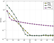
(a) $k=50$

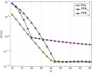
(b) $k=100$

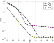
(c) $k=150$

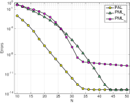
(d) $k=200$

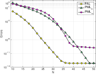
(e) $k=250$

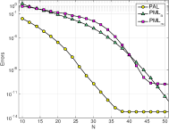
(f) $k=300$

Figure 5.1. A comparation study: PAL vs $\text{PML}_{n}$ vs $\text{PML}_{\infty}$ for various $k=50,100,150,200,250,300.$

In order to study the influence of the thickness of the artificial layer, we keep $R_{1}=2$, vary $R_{2}$ and tabulate in Table 1 the numerical errors for a fixed polynomial degree $(N_{1},N)=(300,30)$ for a large range of $k=(10,50,100,200,300,500).$ It demonstrates that the value of the thickness $d=R_{2}-R_{1}$ has major impact on the accuracy. To optimize the PAL method and achieve high accuracy, a good choice of the thickness turns to be $d=\frac{10}{kR_{1}}.$ We also find the PAL is much less dependent on the choice of $\sigma_{0}$ and $\sigma_{1},$ and it is safe to choose $\sigma_{0}=\sigma_{1}=1,$ which is largely due to the compression of the transformation.

Table 1. Errors vs thickness $d$ for PAL with $(N_{1},N)=(300,30)$

$k$	$d=1$	$d=0.5$	$d=0.1$	$d=0.01$	$d=0.001\!\!$
10	1.11E-12	1.60E-12	1.26E-8	1.39E-4	1.69E-2
50	9.92E-11	4.67E-13	3.27E-12	2.82E-7	5.69E-4
100	2.65E-6	3.79E-11	2.08E-13	1.34E-8	8.65E-5
200	5.72E-4	1.91E-6	9.60E-14	3.12E-10	7.73E-6
300	3.60E-3	7.51E-5	2.65E-13	3.03E-11	1.30E-6
500	1.57E-2	1.40E-3	1.33E-11	1.90E-12	1.68E-7

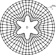
(a) illustration of mesh grids

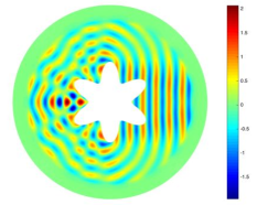
(b) ${\rm Re}(u)$ and ${\rm Re}(v)$

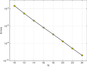
(c) errors of (b) against $N$

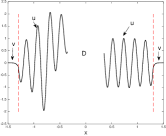
(d) profile along x-axis

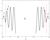
(e) profile along y-axis

Figure 5.2. Hexagonal star-shaped scatterer with an circular PAL layer. The simulation results are obtained with $k=30,$ $\theta_{0}=0,$ $\sigma_{0}=\sigma_{1}=1,$ $(R_{1},R_{2})=(1.3,1.55)$, $N_{1}=35$ and various $N$.

Next, we consider a hexagonal star-shaped scatterer with its boundary radius parameterized by

$$R_{0}(\theta)=0.5+0.15\sin(6(\theta+{\pi}/{4})),\quad\theta=[0,2\pi).$$ (5.3)

The exterior domain is surrounded with an annulus PAL layer with $(R_{1},R_{2})=(1.3,1.55).$ To numerically stimulate this problem, we discretize the computational domain $\Omega\cup\Omega_{\varrho}^{\rm PAL}$ with 250 non-overlapping quadrilateral elements $\Omega=\{\Omega^{(i)}\}_{i=1}^{200}$ and $\Omega_{\varrho}^{\rm PAL}=\{\Omega_{\varrho}^{(i)}\}_{i=1}^{50}$, as shown in Figure 5.2 (a). Once again, the spectral-element scheme is implemented based on Theorem 4.44. Using the Gordon-Hall elemental transformation $\{T^{i},T_{\varrho}^{i}\}:[-1,1]^{2}\mapsto\{\Omega^{(i)},\Omega_{\varrho}^{(i)}\},$ we define the approximation space

$$u_{\boldsymbol{N}}\in V_{\boldsymbol{N}}=\big{\{}u\in H^{1}(\Omega):u|_{\Omega^{(i)}}\circ T^{i}\in\mathbb{P}_{N_{1}}\times\mathbb{P}_{N_{1}},\;u|_{\Omega_{\varrho}^{(i)}}=v_{\boldsymbol{N}}w,\;v_{\boldsymbol{N}}|_{\Omega_{\varrho}^{(i)}}\circ T_{\varrho}^{i}\in\mathbb{P}_{N_{1}}\times\mathbb{P}_{N}\big{\}}.$$ (5.4)

We set $\theta_{0}=0,$ $k=30,$ and $\sigma_{0}=\sigma_{1}=1$. $N_{1}=35$ is employed in all tests, which is large enough to guarantee the numerical errors are mainly induced by the approximation error in the PAL layer. Since the exact solution with irregular scatterer is not available, we adopt the numerical solution obtained by $(N_{1},N)=(35,35)$ as a reference solution and the numerical errors are obtained by comparing the numerical solution with this reference solution. In Figure 5.2 (b), we plot $\Re\{u_{\boldsymbol{N}}\}|_{\Omega}$ and $\Re\{v_{\boldsymbol{N}}\}|_{\Omega_{\varrho}^{\rm PAL}}$ with $(N_{1},N)=(35,15)$. We plot the maximum errors in $\Omega$ against $N$ in Figure 5.2 (c). Observe that the errors decay exponentially as $N$ increases, and the approximation in the layer has no oscillation and is well-behaved, as shown by the profiles along $x$-and $y$-axis of the numerical solution in Figure 5.2 (d)-(e).

5.2. Hexagonal star-shaped layer

(a) illustration of mesh grids

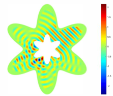
(b) ${\rm Re}(u)$ and ${\rm Re}(v)$

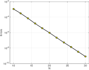
(c) errors of (b) against $N$

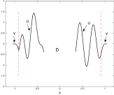
(d) profile along x-axis

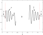
(e) profile along y-axis

Figure 5.3. Hexagonal star-shaped scatterer and PAL layer. The simulation results are obtained with $k=30,$ $\theta_{0}=\pi/4,$ $\sigma_{0}=\sigma_{1}=1,$ $R_{1}(\theta)=2.6R_{0}(\theta)$ and $R_{2}(\theta)=3R_{0}(\theta)$ with $R_{0}(\theta)$ defined in (5.3), $N_{1}=35$ and various $N$.

Next, we surround the same scatterer in the previous example with an hexagonal star-shaped layer, i.e., the parameterized form for the inner and outer radius for the layer are $R_{1}(\theta)=2.6R_{0}(\theta)$ and $R_{2}(\theta)=3R_{0}(\theta)$ with $R_{0}(\theta)$ defined in (5.3). We set $k=30$ and the incident angle $\theta_{0}=\pi/4.$ We partition the computational domain into 250 quadrilateral curvilinear spectral elements, as illustrated in Figure 5.3. We depict $\Re\{u_{\boldsymbol{N}}\}|_{\Omega}$ and $\Re\{v_{\boldsymbol{N}}\}|_{\Omega_{\varrho}^{\rm PAL}}$ with $(N_{1},N)=(35,15)$ in Figure 5.3 (b). The maximum error in $\Omega$ against $N$ is shown in Figure 5.3 (c). It is evident that the errors decrease exponentially with increased polynomial degree $N$, displaying an exponential convergence rate. Figure 5.3 (d)-(e) show the profiles of the numerical solution in Figure 5.3(b) along $x$-and $y$-axis. We observe that the solution profile in the PAL layer smoothly decreases to zero without any oscillation.

5.3. Elliptical layer

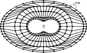
(a) illustration of mesh grids

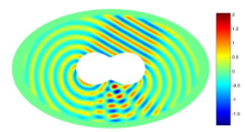
(b) ${\rm Re}(u)$ and ${\rm Re}(v)$

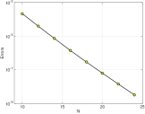
(c) errors of (b) against $N$

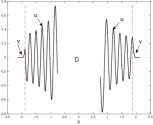
(d) profile along x-axis

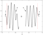
(e) profile along y-axis

Figure 5.4. Peanut-shaped scatterer with elliptical PAL layer. The simulation results are obtained with $k=30,$ $\theta_{0}=\pi/3,$ $\sigma_{0}=\sigma_{1}=1,$ $R_{0}(\theta)$ and $R_{1}(\theta)$ are computed based on (5.5) and (3.9) and $R_{2}(\theta)=\frac{17}{15}R_{1}(\theta)$, $N_{1}=35$ and various $N$.

The geometries of the PAL layer and the scatterer can be rather general. Consider a peanut-shaped scatterer with its boundary radius parameterized by

$$R_{0}(\theta)=0.5+0.25\sin(2(\theta+{\pi}/{4})),\quad\theta=[0,2\pi).$$ (5.5)

The exterior domain is truncated with an elliptical PAL layer with $\Gamma_{\!R_{1}}$ to be an ellipse: $\frac{x^{2}}{a^{2}}+\frac{y^{2}}{b^{2}}=1$ with $a>b>0,$ and $a$ and $b$ take the form

$$a=1.5\cosh(0.7),\quad b=1.5\sinh(0.7).$$

Then $R_{1}(\theta)$ can be computed based on (3.9) and we let $R_{2}(\theta)=\frac{17}{15}R_{1}(\theta)$. We set $k=30$ and $\theta_{0}=\pi/3.$ The numerical scheme are implemented based on Theorem 4.2. The computational domain is partitioned by 200 spectral elements shown in Figure 5.4 (a). $\Re\{u_{\boldsymbol{N}}\}|_{\Omega}$ and $\Re\{v_{\boldsymbol{N}}\}|_{\Omega_{\varrho}^{\rm PAL}}$ obtained with $(N_{1},N)=(35,15)$ are plotted in Figure 5.4. Maximum error against $N$ and the profiles of the numerical solution along $x$-and $y$-axis are depicted, respectively in Figure 5.4 (c)-(f). Due to the well-behaved and non-oscillatory nature of the solution in the PAL layer, the error history exhibits an exponential convergence rate.

5.4. Rectangular layer

Next, we surround the scatterer in the previous example with a rectangular PAL layer with the boundary $\Gamma_{\!R_{1}}$ as a square with four vertices: $(a,b),(-a,b),(-a,-b),$ $(a,-b)$ with $a=1.5$ and $b=0.75.$ Thus, $R_{1}(\theta)$ can be computed by (3.8) and we let $R_{2}(\theta)=\frac{17}{15}R_{1}(\theta).$ In this simulation, the wavenumber and incident angle are set to be $k=30$ and $\theta_{0}=\pi/3$. The domain of interest is discretized into 200 spectral elements, as depicted in Figure 5.5 (a). We plot $\Re\{u_{\boldsymbol{N}}\}|_{\Omega}$ and $\Re\{v_{\boldsymbol{N}}\}|_{\Omega_{\varrho}^{\rm PAL}}$ obtained with $(N_{1},N)=(35,15),$ the maximum error compared with the reference solution obtained with $N_{1}=N=35$, and the profiles of the numerical solution along $x$- and $y$-axis in Figure 5.5 (b)-(f). And it can be observed that the error decreases exponentially as $N$ increases and the solution in the rectangular PAL layer are well-behaved and smoothly decreases to zero with non-oscillatory profiles.

It is also possible to simulate the exterior scattering problem with locally inhomogeneous medium. All the numerical settings are the same except the refraction index $n(\boldsymbol{x})$ in (4.2) in $\Omega$ are replaced by a shifted Guassian function

$$n(\boldsymbol{x})=1+c_{0}\exp\Big{(}-\frac{(x-x_{0})^{2}+(y-y_{0})^{2}}{2c_{1}^{2}}\Big{)}.$$ (5.6)

The inhomogeneous refraction index is depicted in Figure 5.6 (a). Similarly, we demonstrate the real part of the solution in Figure 5.6 (b). Observe that compared with Figure 5.5 (b), the oscillation of the solution field above the upper-middle region of the peanut scatterer increases, due to the influence of the inhomogeneity therein. The maximum error and the profiles of the numerical solution along $x$-and $y$- axis are depicted in Figure 5.6 (c)-(f), respectively. We conclude that the proposed PAL technique is accurate and robust for various scatterers and with locally inhomogeneous medium.

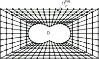
(a) illustration of mesh grids

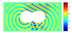
(b) ${\rm Re}(u)$ and ${\rm Re}(v)$

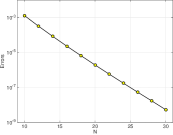
(c) errors of (b) against $N$

(d) profile along x-axis

(e) profile along y-axis

Figure 5.5. Peanut-shaped scatterer with a rectangluar PAL layer. The simulation results are obtained with $k=30,$ $\theta_{0}=\pi/3,$ $\sigma_{0}=\sigma_{1}=1,$ $R_{0}(\theta)$ and $R_{1}(\theta)$ are computed based on (5.5) and (3.8) and $R_{2}(\theta)=\frac{17}{15}R_{1}(\theta)$, $N_{1}=35$ and various $N$.

(a) refraction index $n(\boldsymbol{x})$

(b) ${\rm Re}(u)$ and ${\rm Re}(v)$

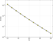
(c) errors of (b) against $N$

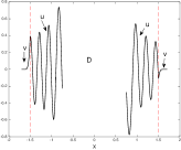
(d) profile along x-axis

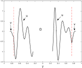
(e) profile along y-axis

Figure 5.6. Scattering problem with a locally inhomogeneous medium with a rectangular PAL. The simulation results are obtained with $k=30,$ $\theta_{0}=\pi/3,$ $\sigma_{0}=\sigma_{1}=1,$ $R_{0}(\theta)$ and $R_{1}(\theta)$ are computed based on (5.5) and (3.8) and $R_{2}(\theta)=\frac{17}{15}R_{1}(\theta)$, $N_{1}=35$ and various $N$.

Appendix A Proof of Theorem 2.1

For clarity, we first consider (2.1) with $g(y)=\hat{g}_{l}\sin(ly),$ and then apply the principle of superposition to obtain (2.11). Note that by (2.3), the exact solution of (2.1) is

$$U_{l}(x,y)=\hat{g}_{l}\,e^{{\rm i}\hat{k}_{l}x}\sin(ly),$$ (A.1)

and the PML-solution of (2.8)-(2.9) is

$$U_{{\rm p},l}(x,y)=\frac{e^{{\rm i}\hat{k}_{l}(S_{d}-S)}-e^{-{\rm i}\hat{k}_{l}(S_{d}-S)}}{e^{{\rm i}\hat{k}_{l}S_{d}}-e^{-{\rm i}\hat{k}_{l}S_{d}}}\,\hat{g}_{l}\sin(ly).$$ (A.2)

In fact, one verifies directly that (A.2) satisfies the PML-equation (2.8) and all conditions in (2.10)-(2.9). Since $S(x)=x$ for $x\in(0,L),$ we find

$$U_{{\rm p},l}(x,y)=\frac{e^{{\rm i}\hat{k}_{l}(S_{d}-2x)}-e^{-{\rm i}\hat{k}_{l}S_{d}}}{e^{{\rm i}\hat{k}_{l}S_{d}}-e^{-{\rm i}\hat{k}_{l}S_{d}}}\,U_{l}(x,y)=(1-R_{l}(x))\,U_{l}(x,y),\;\;\;\forall\,(x,y)\in\Omega,$$ (A.3)

where the representation of $R_{l}(x)$ in (2.11) can be obtained straightforwardly. Thanks to the identity (A.3), we derive from the principle of superposition, (2.3) and (A.1) that the PML-solution in $\Omega$ is given by

$$U_{\rm p}(x,y)=\sum_{l=1}^{\infty}U_{{\rm p},l}(x,y)=U(x,y)-\sum_{l=1}^{\infty}\hat{g}_{l}\,R_{l}(x)\,e^{{\rm i}\hat{k}_{l}x}\sin(ly),$$ (A.4)

which yields (2.11).

It remains to derive the bounds in (2.13). One verifies readily that for $z=\alpha+\beta\,{\rm i}$ with $\alpha,\beta\in{\mathbb{R}},$

$$\begin{split}&|1-e^{\alpha}|\leq|1-e^{z}|\leq 1+e^{\alpha},\quad|\sin z|=\Big{|}\frac{e^{{\rm i}z}-e^{-{\rm i}z}}{2{\rm i}}\Big{|}=\frac{e^{-\beta}}{2}|1-e^{-2{\rm i}z}|.\end{split}$$ (A.5)

Then we have

$$|1-e^{2{\rm Im}\{\hat{k}_{l}S_{d}\}}|\leq|{1-e^{-2{\rm i}\hat{k}_{l}S_{d}}}|\leq 1+e^{2{\rm Im}\{\hat{k}_{l}S_{d}\}}.$$ (A.6)

Therefore, (i) for $k>l$ (note $\hat{k}_{l}=\sqrt{k^{2}-l^{2}}$), we obtain (2.13) from (A.5)-(A.6) immediately.

On the other hand, (ii) for $k<l$ (note $\hat{k}_{l}={\rm i}|\hat{k}_{l}|$), the lower and upper bounds in (2.14) are a direct consequence of (A.6).

If $k$ is a positive integer, we find that for the mode $l=k,$ (A.1) is still valid (i.e., $U_{l}=\hat{g}_{l}\sin(ly)$), while (A.2) becomes

$$U_{{\rm p},l}(x,y)=\Big{(}1-\frac{S(x)}{S_{d}}\Big{)}\,\hat{g}_{l}\,\sin(ly).$$ (A.7)

Thus, for the mode $l=k,$ $R_{l}(x)$ should be replaced by $R_{l}(x)=-S(x)/S_{d}$ in the identity (2.11).

Appendix B Proof of Theorem 4.1

Proof.

Without loss of generality, we start with a general nonsingular Cartesian coordinate transformation: $\tilde{x}=X(x,y),\;\tilde{y}=Y(x,y),$ with Jacobian and Jacobian matrix given by

$$\boldsymbol{J}=\frac{\partial(x,y)}{\partial(\tilde{x},\tilde{y})}=\frac{1}{{\rm det}(\boldsymbol{J})}\begin{pmatrix}Y_{y}&-X_{y}\\[1.0pt] -Y_{x}&X_{x}\\[1.0pt] \end{pmatrix},\quad{\rm det}(\boldsymbol{J})=X_{x}Y_{y}-X_{y}Y_{x}\not=0.$$ (B.1)

It is known from the standard text book that (4.4) can be transformed into

$$\mathcal{H}[U]=\frac{1}{n}\big{\{}\nabla\cdot(\boldsymbol{C}\,\nabla U)+k^{2}n\,U\big{\}},$$ (B.2)

where $U(x,y)=\tilde{U}(\tilde{x},\tilde{y})$ and

$${\boldsymbol{C}}=\begin{pmatrix}C_{11}&C_{12}\\ C_{12}&C_{22}\end{pmatrix}=\frac{{\boldsymbol{J}}\,\boldsymbol{J}^{t}}{{\rm det}(\boldsymbol{J})},\quad n=\frac{1}{{\rm det}(\boldsymbol{J})}.$$ (B.3)

To represent $\boldsymbol{J}$ and its determinant in polar coordinates, we rewrite the above nonsingular transformation as $\tilde{r}=R(r,\theta),\,\tilde{\theta}=\Theta(r,\theta).$ Then by the chain rule, we have

$$\frac{\partial(x,y)}{\partial(\tilde{x},\tilde{y})}\frac{\partial(\tilde{x},\tilde{y})}{\partial(x,y)}=\frac{\partial(\tilde{x},\tilde{y})}{\partial(\tilde{r},\tilde{\theta})}\frac{\partial(\tilde{r},\tilde{\theta})}{\partial(\tilde{x},\tilde{y})}=\frac{\partial(r,\theta)}{\partial(x,y)}\frac{\partial(x,y)}{\partial(r,\theta)}=\boldsymbol{I}_{2}.$$

As a result, the matrix $\boldsymbol{J}$ can be computed by

$$\begin{split}\boldsymbol{J}&=\frac{\partial(x,y)}{\partial(\tilde{x},\tilde{y})}=\bigg{(}\frac{\partial(\tilde{x},\tilde{y})}{\partial(x,y)}\bigg{)}^{-1}=\bigg{(}\frac{\partial(\tilde{x},\tilde{y})}{\partial(\tilde{r},\tilde{\theta})}\frac{\partial(\tilde{r},\tilde{\theta})}{\partial(r,\theta)}\frac{\partial(r,\theta)}{\partial(x,y)}\bigg{)}^{-1}\\ &=\frac{\partial(x,y)}{\partial(r,\theta)}\bigg{(}\frac{\partial(\tilde{r},\tilde{\theta})}{\partial(r,\theta)}\bigg{)}^{-1}\frac{\partial(\tilde{r},\tilde{\theta})}{\partial(\tilde{x},\tilde{y})}.\end{split}$$ (B.4)

Straightforward calculation leads to

$$\frac{\partial(x,y)}{\partial(r,\theta)}=\boldsymbol{T}(\theta)\begin{pmatrix}1&0\\ 0&r\end{pmatrix},\;\quad\frac{\partial(\tilde{r},\tilde{\theta})}{\partial(\tilde{x},\tilde{y})}=\begin{pmatrix}1&0\\ 0&1/\tilde{r}\end{pmatrix}\boldsymbol{T}^{t}(\tilde{\theta}),$$ (B.5)

and

$$\frac{\partial(\tilde{r},\tilde{\theta})}{\partial(r,\theta)}=\begin{pmatrix}R_{r}&R_{\theta}\\ \Theta_{r}&\Theta_{\theta}\end{pmatrix},\quad\;\;\Big{(}\frac{\partial(\tilde{r},\tilde{\theta})}{\partial(r,\theta)}\Big{)}^{-1}=\frac{1}{R_{r}\Theta_{\theta}-R_{\theta}\Theta_{r}}\begin{pmatrix}\Theta_{\theta}&-R_{\theta}\\ -\Theta_{r}&R_{r}\end{pmatrix}.$$ (B.6)

Inserting (B.5)-(B.6) into (B.4), and using the property: ${\rm det}(\boldsymbol{T}(\theta))={\rm det}(\boldsymbol{T}(\tilde{\theta}))=1,$ we find

$${\rm det}(\boldsymbol{J})=\frac{r}{R(R_{r}\Theta_{\theta}-R_{\theta}\Theta_{r})},\quad\boldsymbol{J}={{\rm det}(\boldsymbol{J})}\,{\boldsymbol{T}}(\theta)\begin{pmatrix}R\Theta_{\theta}/r&-R_{\theta}/r\\[1.0pt] -R\Theta_{r}&R_{r}\\[1.0pt] \end{pmatrix}{\boldsymbol{T}}^{t}(\Theta).$$ (B.7)

We now apply the above general formulas to (4.1), that is, $\tilde{r}=R=S(r,\theta),\;\tilde{\theta}=\Theta=\theta,$ so $R_{r}=S_{r},R_{\theta}=S_{\theta},\Theta_{r}=0,\Theta_{\theta}=1.$ Then we obtain immediately from (B.7) that

$${\rm det}({\boldsymbol{J}})=\frac{r}{SS_{r}},\quad{\boldsymbol{J}}={\boldsymbol{T}}(\theta)\begin{pmatrix}\frac{1}{S_{r}}&-\frac{S_{\theta}}{SS_{r}}\\[4.0pt] 0&\frac{r}{S}\end{pmatrix}{\boldsymbol{T}}^{t}(\theta).$$ (B.8)

Then, ${\boldsymbol{C}}$ and $n$ in (4.6) can be derived directly from (B.3) and (B.8). This ends the proof. ∎

References

- [1] M. Abramovitz and I.A. Stegun. Handbook of Mathematical Functions. Dover, New York, 1972.
- [2] S. Amini and S.M. Kirkup. Solution of Helmholtz equation in the exterior domain by elementary boundary integral methods. J. Comp. Phys., 118(2):208–221, 1995.
- [3] A. Bayliss and E. Turkel. Radiation boundary conditions for wave-like equations. Comm. Pure Appl. Math., 33:707–725, 1980.
- [4] J.P. Berenger. A perfectly matched layer for the absorption of electromagnetic waves. J. Comput. Phys., 114(2):185–200, 1994.
- [5] J.P. Berenger. Perfectly matched layer for the FDTD solution of wave-structure interaction problems. IEEE Trans. Antennas and Propag., 44(1):110–117, 1996.
- [6] J.P. Berenger. Three-dimensional perfectly matched layer for the absorption of electromagnetic waves, J. Comput. Phys., 114: 363–379, 1996.
- [7] A. Bermúdez, L. Hervella-Nieto, A. Prieto, and R. Rodríguez. An exact bounded perfectly matched layer for time-harmonic scattering problems. SIAM J. Sci. Comp., 30(1):312–338, 2007.
- [8] A. Bermúdez, L. Hervella-Nieto, A. Prieto, and R. Rodríguez. An optimal perfectly matched layer with unbounded absorbing function for time-harmonic acoustic scattering problems. J. Comp. Phys., 223(2):469–488, 2007.
- [9] J.P. Boyd, Chebyshev and Fourier Spectral Methods, Dover Publications Inc., Mineola, NY, second ed., 2001.
- [10] Z.M. Chen and X.Z. Liu. An adaptive perfectly matched layer technique for time-harmonic scattering problems. SIAM J. Numer. Anal., 43(2):645–671, 2005.
- [11] Z.M. Chen and X.M. Wu. An adaptive uniaxial perfectly matched layer method for time-harmonic scattering problems. Numer. Math. Theor. Meth. Appl, 1: 113–137, 2008.
- [12] Z.M. Chen, T. Cui and L.B. Zhang. An adaptive anisotropic perfectly matched layer method for 3-D time harmonic electromagnetic scattering problems. Numer. Math., 125(4):639–677, 2013.
- [13] Z.M. Chen and W.Y. Zheng. PML method for electromagnetic scattering problem in a two-layer medium. SIAM J. Numer. Anal., 55(4):2050–2084, 2017.
- [14] W.C. Chew and W.H. Weedon. A 3D perfectly matched medium from modified Maxwell’s equations with stretched coordinates. Microw. Opt. Technol. Lett., 7(13):599–604, 1994.
- [15] R. Cimpeanu, A. Martinsson, and M. Heil. A parameter-free perfectly matched layer formulation for the finite-element-based solution of the Helmholtz equation. J. Comput. Phys., 296: 329–47, 2015.
- [16] F. Collino and P. Monk. The perfectly matched layer in curvilinear coordinates. SIAM J. Sci. Comput., 19(6):2061–2090, 1998.
- [17] D. Colton and R. Kress. Integral Equation Methods in Scattering Theory. SIAM, 2013.
- [18] A. Darvish, B. Zakeri and N. Radkani. An optimized hybrid convolutional perfectly matched layer for efficient absorption of electromagnetic waves. J. Comput. Phys., 356: 31-45, 2018.
- [19] C. Deng, M. Luo, M. Yuan, B. Zhao, M. Zhuang, and Q.H. Liu. The auxiliary differential equations perfectly matched layers based on the hybrid SETD and PSTD algorithms for acoustic waves. J. Comput. Acoustics, 26:1750031 (19 pages), 2017.
- [20] M.O. Deville, P.F. Fischer, and E.H. Mund. High-Order Methods for Incompressible Fluid Flow, volume 9. Cambridge University Press, 2002.
- [21] B. Engquist and A. Majda. Absorbing boundary conditions for numerical simulation of waves. Math. Comp., 31:629–651, 1977.
- [22] K. Feng. Finite element method and natural boundary reduction. Proceeding of ICM, Warsaw, 1439–1453, 1983.
- [23] N. Feng, Y. Yue, C. Zhu, L. Wan, and Q. H. Liu. Second-order PML: Optimal choice of th-order PML for truncating FDTD domains. J. Comput. Phys., 285: 71–83, 2015.
- [24] A. Fournier. Exact calculation of Fourier series in nonconforming spectral-element methods. J. Comput. Phys., 215:1–5, 2006
- [25] D. Givoli. Non-reflecting boundary conditions. J. Comp. Phys., 94:1–29, 1991.
- [26] D. Givoli. High-order non-reflecting boundary scheme for time-dependent waves. J. Comp. Phys., 186(1):24–46, 2003.
- [27] C.I. Goldstein. A finite element method for solving Helmholtz type equations in waveguides and other unbounded domains. Math. Comp., 39(160):309–324, 1982.
- [28] W.J. Gordon and C.A. Hall. Transfinite element methods: blending-function interpolation over arbitrary curved element domains. Numer. Math., 21(2):109–129, 1973.
- [29] B.Y. Guo. Gegenbauer approximation and its applications to differential equations with rough asymptotic behaviors at infinity. Appl. Numer. Math., 38 (4): 403–425, 2001.
- [30] T. Hagstrom. Radiation boundary conditions for the numerical simulation of waves. Acta Numer., 8:47–106, 1999.
- [31] T. Hagstrom and L. Stephen. Radiation boundary conditions for Maxwell’s equations: a review of accurate time-domain formulations. J. Comput. Math., 25:305–336, 2007.
- [32] S. Johnson. Notes on perfectly matched layers. Technical report, Massachusetts Institute of Technology, Cambridge,MA, 2010.
- [33] M. Lassas and E. Somersalo. On the existence and convergence of the solution of PML equations. Computing, 60(3):229–241, 1998.
- [34] Y. Li and H. Wu. FEM and CIP-FEM for Helmholtz equation with high wave number and perfectly matched layer truncation. SIAM J. Numer. Anal., 57(1), 96–126, 2019.
- [35] P. Loh, A. Oskooi, M. Ibanescu, M. Skorobogatiy, and S. Johnson. Fundamental relation between phase and group velocity, and application to the failure of perfectly matched layers in backward-wave structures. Phys. Rev. E, 79(6):065601, 2009.
- [36] J. B. Pendry, D. Schurig, and D. R. Smith. Controlling electromagnetic fields. Science, 312(5781):1780–1782, 2006.
- [37] A. Modave, E. Delhez, and C. Geuzaine. Optimizing perfectly matched layers in discrete contexts. Int. J. Numer. Methods Eng., 99(6): 410–437, 2014.
- [38] J.C. Nédélec. Acoustic and Electromagnetic Equations. Springer-Verlag, New York, 2001.
- [39] D. Rabinovich, D. Givoli, and E. Bécache. Comparison of high-order absorbing boundary conditions and perfectly matched layers in the frequency domain. Int. J. Numer. Meth. Eng., 26(10):1351–1369, 2010.
- [40] C. Radu, M. Anton, and H. Matthias. A parameter-free perfectly matched layer formulation for the finite-element-based solution of the Helmholtz equation. J. Comput. Phys., 296:329–347, 2015.
- [41] J. Shen, T. Tang, and L.L. Wang. Spectral Methods: Algorithms, Analysis and Applications. Vol. 41, Springer, Berlin, 2011.
- [42] J. Shen and L.L. Wang, Some recent advances on spectral methods for unbounded domains. Commun. Comp. Phys., 5: 195–241, 2009.
- [43] I. Singer and E. Turkel. A perfectly matched layer for the Helmholtz equation in a semi-infinite strip. J. Comp. Phys., 201(2):439–465, 2004.
- [44] Q. Sun, R. Zhang, Q. Zhan, and Q.H. Liu. A novel coupling algorithm for perfectly matched layer with wave equation-based discontinuous Galerkin time-domain method. IEEE Trans. Antennas Propag., 66(1):255–261, 2018.
- [45] A. Taflove and S. Hagness. Computational Electrodynamics: the Finite-Difference Time-Domain Method. Artech House, Inc., Boston, MA, third edition, 2005. With 1 CD-ROM (Windows).
- [46] B. Wang, L.L. Wang and Z. Xie. Accurate calculation of spherical and vector spherical harmonic expansions via spectral element grids. Adv. Comput. Math., 44(2), 951–985, 2018.
- [47] L.L. Wang and Z.G. Yang. A perfect absorbing layer for high-order simulation of wave scattering problems. Spectral and High Order Methods for Partial Differential Equations, M.L. Bittencourt et al. (eds.), pp. 81-101, 2017, Springer. Invited papers for the ICOSAHOM2016, Rio de Janeiro, Brazil, June 27-July 1, 2016.
- [48] W. Yang, J. Li, and Y. Huang. Mathematical analysis and finite element time domain simulation of arbitrary star-shaped electromagnetic cloaks. SIAM J. Numer. Anal., 56(1): 136–159, 2018.
- [49] Z.G. Yang and L.L. Wang. Accurate simulation of circular and elliptic cylindrical invisibility cloaks. Commun. Comput. Phys., 17(03):822–849, 2015.
- [50] Z.G. Yang, L.L. Wang, Z.J. Rong, B. Wang, and B.L. Zhang. Seamless integration of global Dirichlet-to-Neumann boundary condition and spectral elements for transformation electromagnetics. Comput. Meth. Appl. Mech. Eng., 301:137–163, 2016.
- [51] N.A. Zharova, L.V. Shadrivov, and Y.S. Kivshar. Inside-out electromagnetic cloaking. Opt. Express, 16(7):4615–4620, 2008.
- [52] W. Zhou and H. Wu. An adaptive finite element method for the diffraction grating problem with PML and few-mode DtN truncations, J. Sci. Comput., 76(3): 1813–1838, 2018.