Speech-Based Parameter Estimation of an Asymmetric Vocal Fold Oscillation Model and Its Application in Discriminating Vocal Fold Pathologies

Abstract

So far, several physical models have been proposed for the study of vocal fold oscillations during phonation. The parameters of these models, such as vocal fold elasticity, resistance, etc. are traditionally determined through the observation and measurement of the vocal fold vibrations in the larynx. Since such direct measurements tend to be the most accurate, the traditional practice has been to set the parameter values of these models based on measurements that are averaged across an ensemble of human subjects. However, the direct measurement process is hard to revise outside of clinical settings. In many cases, especially in pathological ones, the properties of the vocal folds often deviate from their generic values—sometimes asymmetrically wherein the characteristics of the two vocal folds differ for the same individual. In such cases, it is desirable to find a more scalable way to adjust the model parameters on a case by case basis. In this paper, we present a novel and alternate way to determine vocal fold model parameters from the speech signal. We focus on an asymmetric model and show that for such models, differences in estimated parameters can be successfully used to discriminate between voices that are characteristic of different underlying vocal fold pathologies.

Index Terms—  Asymmetric vocal fold models, vocal fold parameterization, voice pathologies, voice profiling, nonlinear dynamics

1 Introduction

Phonation is the process wherein the vocal folds in the larynx are set into a state of self-sustained vibration, causing an excitation signal to be produced at the glottal source. This signal resonates in the vocal tract of the speaker and, depending on the shape of the vocal tract and the configuration of the articulators (tongue, lip, jaw, etc.), is heard as a characteristic voiced sound by the listener. Phonation is thus important in the production of all vowels and all voiced consonants in all languages of the world.

As per the myoelastic-aerodynamic theory of phonation, the self-sustained vibrations of the vocal folds are initiated and driven by a delicate balance of physical and aerodynamic forces across the glottis [1]. The actual movements are governed by various biomechanical properties of the vocal folds such as elasticity, resistance, Young’s modulus, viscosity, etc. In pathological cases such as vocal palsy, phonotrauma, neoplasm, etc., these properties of the vocal structures vary from their generic settings  [2]. These often cause the movements of the vocal folds to become asymmetric [3]—where the movements of the left and right folds are out of sync—in a manner that is characteristic of the underlying pathology.

The premise of our paper is that if these movements of the vocal folds and the underlying parameters of the system that produces them could be recovered from the speech signal, the underlying pathologies too could be identified. In order to do so, we must consider the actual physics of the vocal-fold movements, how they influence its movements, and how these manifest in the speech signal itself.

The exact physics of the airflow through the glottis during phonation is well studied, e.g., [4, 5, 6, 7, 8, 9], and a number of physical models have been proposed for it, e.g., [5, 10, 11, 12, 13, 14, 15, 16]. The models use measured biomechanical properties of the vocal folds within a set of equations that capture the movements of the glottis during phonation. Since the vocal fold dynamics are non-linear, the models are systems of coupled non-linear dynamical equations as well. They output a phase space trajectory of state variables that describes the movements of the folds. The trajectories tend to fall into orbits with regular or irregular behaviors, which actually explain observed behavior patterns of the vocal folds. The possible types and distributions of these orbits depend on the system parameters. To explain asymmetric movements of vocal folds, such as those seen under pathologies, asymmetric dynamical models of the vocal folds have been proposed that are able to emulate these asymmetric vibratory motions of the vocal folds [17].

While these models effectively solve the forward problem of accurately emulating vocal fold movements during phonation, the reverse problem of finding the correct model parameters given a set of observed vocal fold movements has not been addressed. We develop a methodology to solve it based on the analysis of the speech signal. Given a model for asymmetric movements of the vocal folds and a set of speech signals from people affected by various pathologies that affect vocal fold movements, we propose a method to estimate the parameters of the asymmetric model that explains them. We further show how the re-estimated model parameters can be mapped into the phase space of the nonlinear dynamical systems, and how the location of these parameters in the parameter space of the model can directly indicate the underlying pathology in the observed speech signal.

2 Phonation and the vocal folds model

At the biomechanical level, phonation happens as a result of a specific pattern of events in the glottal region. The vocal folds are membranes that are set into vibratory motion as a result of a complex interplay of forces in the vocal tract. These relate to a) pressure balances and airflow dynamics within the supra-glottal and sub-glottal regions, and b) muscular control within the glottis and the larynx. Specifically, during phonation, the vocal folds can vibrate hundreds of times per second. Such oscillations are self-sustained, a physical process driven by the right balance of opposing forces acting on it and set into motion as a result of a chain of events in the laryngeal region [6]. The balance of forces necessary to cause self-sustained vibrations is created by two physical phenomena: the Bernoulli effect and the Coandǎ effect. Figure 1 illustrates the interaction between these effects that drives the oscillations of the vocal folds.

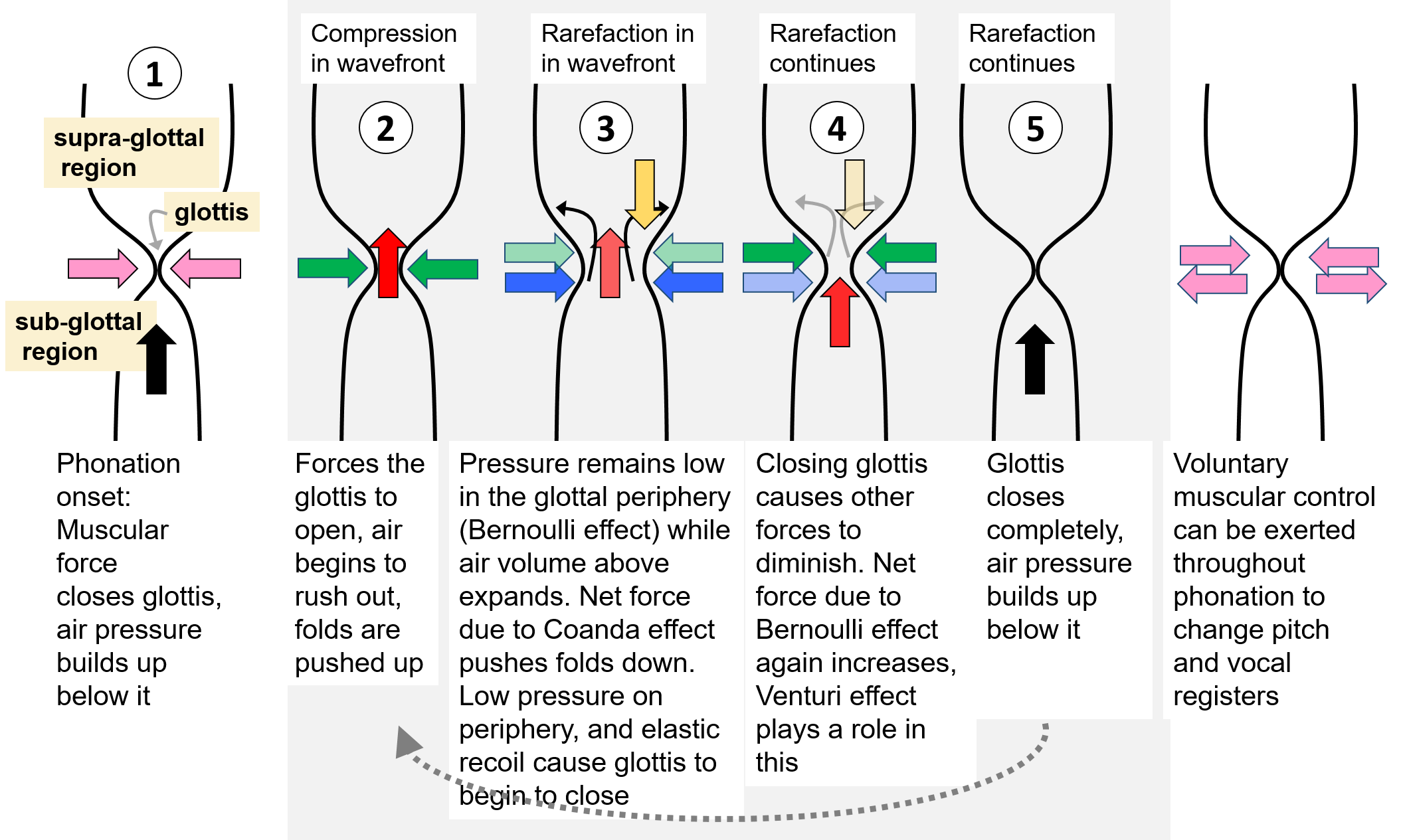
Fig. 1: Schematic of the balance of forces through one cycle of the self-sustained vibrations of the vocal cords. The color codes for the arrows depict net forces due to the following: Pink–muscular; Green–Bernoulli effect; Yellow–Coandǎ effect; Blue–vocal fold elasticity and other factors; Black and Red–air pressure. Lighter shades of each color depict lower forces. Figure from [16] with permission.

2.1 The asymmetric vocal folds oscillation model

To model phonation, computational models of vocal folds have been developed, including four broad types: $1$-mass models, e.g. [11], $2$-mass models, e.g. [5, 10], multi-mass models [13], and finite element models [12]. Each of these have proven to be useful in different contexts. For the purpose of this study, the $1$-mass body-cover model [6, 18, 19, 20] is of particular interest. It assumes that a glottal flow-induced mucosal wave travels upwards within the transglottal region, causing a small displacement of the mucosal tissue, which attenuates down within a few millimeters into the tissue as an energy exchange happens between the airstream and the tissue [6]. This allows us to represent the mucosal wave as a one-dimensional surface wave on the mucosal surface (the cover), and treat the remainder of the vocal folds (the body) as a single mass or safely neglect it. Under this assumption, the oscillation model can be linearized, and the oscillatory conditions are much simplified while maintaining the accuracy of the model.

In most vocal pathologies, it has been observed that the vocal fold vibrations are not symmetrical [14]. Thus the asymmetric vocal fold model is ideally suited to modeling the pathological phonation. We adopt the specific formulation of the $1$-mass asymmetric model from [20]. This model incorporates an asymmetry parameter, which describes the asymmetry in the oscillation of left and right vocal folds. The key assumptions made in formulating this model are: a) the degree of asymmetry is independent of the oscillation frequency, b) the glottal flow is stationary, frictionless and incompressible, c) the effect of source-vocal tract interaction is eliminated, d) there is no glottal closure and hence no vocal fold collision during the oscillation cycle, and e) the small-amplitude body-cover model is applicable.

Following [20] denote the center-line of the glottis as the $z$-axis. At the midpoint ($z=0$) of the thickness of the vocal folds, the left and right vocal folds oscillate with lateral displacement $\xi_{l}$ and $\xi_{r}$, resulting in a pair of coupled Van der Pol oscillators

$$\ddot{\xi}_{r}+\beta(1+\xi_{r}^{2})\dot{\xi}_{r}+\xi_{r}-\frac{\Delta}{2}\xi_{r}=\alpha(\dot{\xi}_{r}+\dot{\xi}_{l})$$

$$\ddot{\xi}_{l}+\beta(1+\xi_{l}^{2})\dot{\xi}_{l}+\xi_{l}+\frac{\Delta}{2}\xi_{l}=\alpha(\dot{\xi}_{r}+\dot{\xi}_{l}),$$ (1)

where $\beta$ is the coefficient incorporating mass, spring and damping coefficients, $\alpha$ is the glottal pressure coupling coefficient, and $\Delta$ is the asymmetry coefficient. For a male adult with normal voice, the reference values for the model parameters may be $\alpha=0.5$, $\beta=0.32$ and $\Delta=0$.

3 Phase space of the asymmetric model

To study the behaviors of nonlinear dynamical systems such as (1), we introduce some useful concepts and tools. The output variables of a dynamical system are also referred to as state variables, as they identify the current state of the system. The phase space of a system is the space whose coordinates are its state variables. We can denote such system as $(T,M,\Phi)$, where $T={\mathbb{R}}_{\geq 0}$ is non-negative real time, the phase space $M$ is a differentiable manifold, and $\Phi:T\times M\supseteq U\to M$ is a continuous evolution function. As the system evolves through time, the map $\Phi_{x}:T\to M$ is the flow or trajectory through $x\in M$, and the set of all flows $\gamma_{x}\coloneqq\{\Phi_{x}:t\in T\}$ is the orbit of $x$ [21].

The behaviors of flows can be described by attractors—a set $A\subseteq M$ that “traps” the orbit $\gamma_{x}$, i.e., starting from initial point $x$, there exists a $t_{0}$ such that $\Phi_{x}(t)\in A$ for $t>t_{0}$. The simplest attractor is an equilibrium point. But we are particularly interested in those attractors revealing the periodic motion of the flow in phase space. Such attractors include the limit cycle or the limit torus, which is an isolated periodic or toroidal orbit. Some other attractors are chaotic, whose trajectories diverge with arbitrarily close initial positions [22, 23]. The phase space of the system may include multiple attractors, the number, location, and type of which depend on its parameters.

Periodic attractors reveal the stability of the system. To dissect the structure of attractors, we use the Poincaré map. For an $n$-dimensional phase space with a periodic orbit $\gamma_{x}$, a Poincaré section $S$ is an $(n-1)$-dimensional section (hyper-plane) transversal to $\gamma_{x}$, and the Poincaré map on $S$ is a map $P:S\supseteq U\to S$, $x\mapsto\Phi_{x}(t_{s})$, where $t_{s}$ is the time between two intersections [21]. We also want to study how the topological structure, including attractors, of phase space change with system parameters. This leads to the study of bifurcation, which occurs when a small change of a model parameter causes an abrupt change of the topological structure. A bifurcation diagram is a visualization of the parameter space of the system showing the number (and behavior) of attractors at each parameter setting.

3.1 Physical interpretation of phase space of asymmetric model

Back to our context, the dynamical system of concern is the asymmetric vocal folds model (1). Its phase space, which is four-dimensional, includes states $(\xi_{r},\dot{\xi}_{r},\xi_{l},\dot{\xi}_{l})$. For this nonlinear system, it is expected that attractors such as limit cycles or toruses will appear in the phase space. Such phenomena are consequences of specific parameter settings. Specifically, the parameter $\beta$ determines the periodicity of oscillations; the parameter $\alpha$ and $\Delta$ quantify the asymmetry of the displacement of left and right vocal folds and the degree to which one of the vocal folds is out of phase with the other [3, 20]. We can visualize them by plotting the left and right displacements as well as the phase space portrait.

The coupling of right and left oscillators is described by their entrainment; they are in $n:m$ entrainment if their phase $\theta_{r}$, $\theta_{l}$ satisfy $|n\theta_{r}-m\theta_{l}|<C$ where $n,m$ are integers and $C$ is a constant [20]. Such entrainment can be shown by the Poincaré map, where the number of crossings of the trajectory of right or left oscillator with the Poincaré section shows the periodicity of its limit cycles. Therefore, their ratio represents the entrainment. To show how the entrainment changes with parameters, we plot the bifurcation diagram. An example of such a bifurcation diagram is shown in Figure 2 [3, 10].

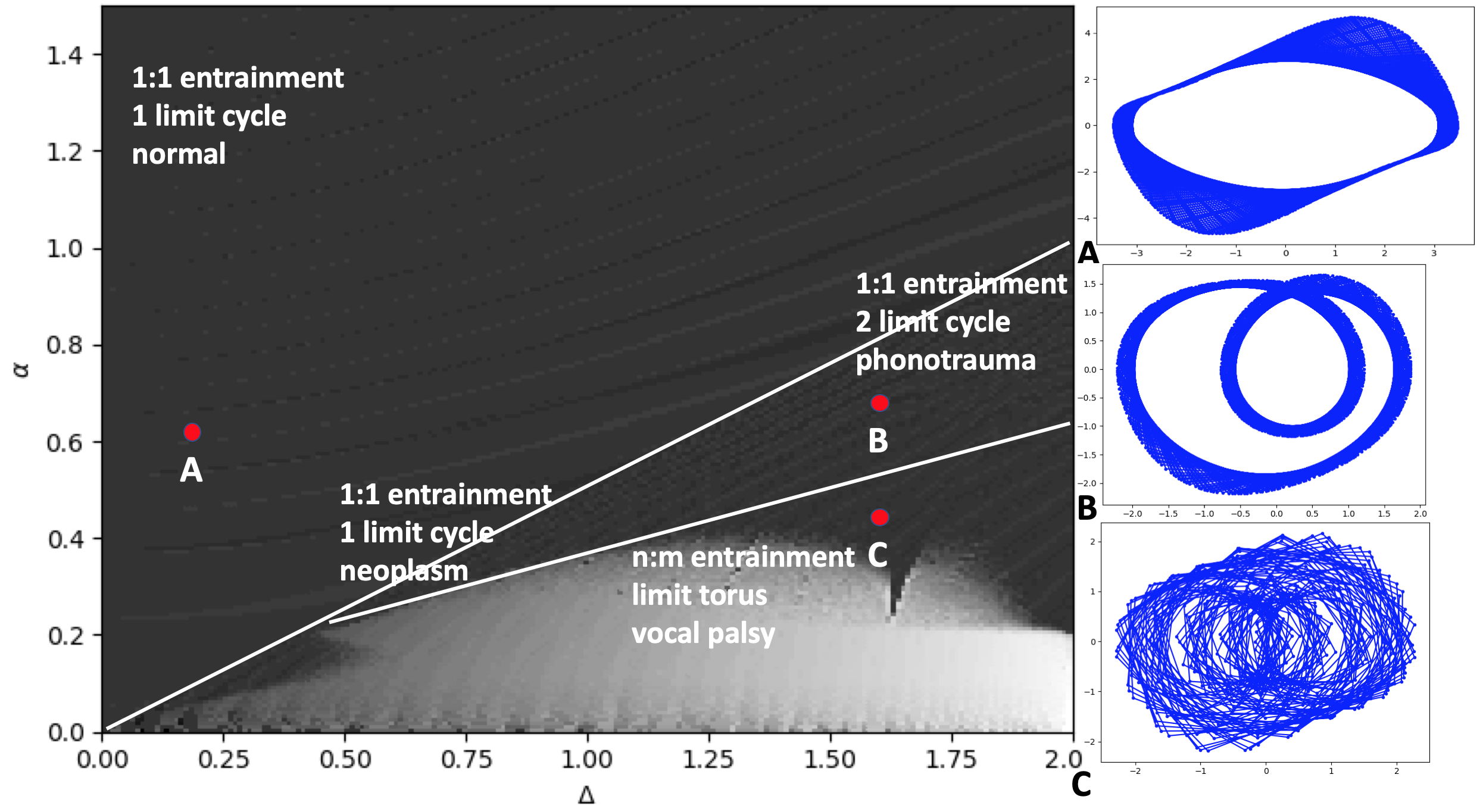
Fig. 2: Bifurcation diagram of the asymmetric vocal fold model. It shows the entrainment ratio $n:m$ (coded as different shades) as a function of model parameter $\alpha$ and $\Delta$, where $n$ and $m$ are the number of intersections of the orbits of right and left oscillators across the Poincaré section $\dot{\xi}_{r,l}=0$ at stable status. This is consistent with the theoretical results in [20]. The phase portraits for point A, B, C are shown alongside, where the horizontal axis is displacement, and the vertical axis is velocity.

As we will see later (and as indicated in Figure 2), model parameters can characterize voice pathologies, which will also be visible in phase portrait and bifurcation plots.

4 Parameter estimation for the model

Finding the parameters of any physical model that emulates vocal fold oscillations is not trivial. For this, one must acquire measurements of the vocal fold displacements, which in turn require either high-speed photography [24] or physical or numerical simulations [12, 25], which are often not easily accessible. Even with the measurements, estimating the model parameters remains hard. The problem itself is commonly termed as the inverse problem [26], and is usually solved via iterative matching procedures [27, 28, 29], stochastic optimization or heuristic procedures [13, 30].

We propose a method for solving the inverse problem that bypasses the difficulties inherent in traditional methods: namely that of either obtaining direct measurements of vocal fold displacements or of the complexity of solving inverse problems using traditional methods. Our proposed solution comprises an Adjoint Least-Squares method, which we call ADLES for brevity, to estimate model parameters directly from speech measurements.

First, we formulate our objective. The vibration of vocal folds oscillates the air particles at the glottal region, producing a pressure wave that propagates through the upper vocal channel into the open air. This pressure wave is considered planar when its frequency is under $4$ KHz [31], and hence a function of position $x\in\varOmega\coloneqq[0,L]$ and time $t\in{\mathcal{T}}\coloneqq[0,T]$—$p(x,t)\in{\mathcal{L}}^{2}(\varOmega\times{\mathcal{T}})$, where $L$ is the length of the upper vocal channel. The acoustic pressure $p_{L}(t)\coloneqq p(L,t)$, which represents the speech signal measured by a microphone near the mouth, is a result of the pressure wave $p_{0}(t)\coloneqq p(0,t)$ at the glottis modulated by the upper vocal channel. If we denote the effect of upper vocal channel as a filter

$${\mathcal{F}}: {\mathcal{L}}^{2}(T)\to{\mathcal{L}}^{2}(T)$$ (2)

$$p_{0}(t)\mapsto p_{L}(t),$$ (3)

we can deduce $p_{0}(t)$ from $p_{L}(t)$ using inverse filtering [32]

$$p_{0}(t)={\mathcal{F}}^{-1}(p_{L}(t)).$$ (4)

Let $A(x)$ be the area function of the vocal channel for $x\in[0,L]$ and $A(0)$ represent the cross-sectional area at the glottis. The corresponding volume velocity $u_{0}(t)$ through the vocal channel is given by

$$u_{0}(t)=\frac{A(0)}{\rho c}p_{0}(t),$$ (5)

where $c$ is the speed of sound and $\rho$ is the ambient air density. As a result, given a measured speech signal $p_{m}(t)$, we have

$$u_{0}^{m}(t)=\frac{A(0)}{\rho c}{\mathcal{F}}^{-1}(p_{m}(t)).$$ (6)

Alternatively, we can derive $u_{0}(t)$ from the displacement of vocal folds by

$$u_{0}(t)=\tilde{c}d\left(2\xi_{0}+\xi_{l}(t)+\xi_{r}(t)\right),$$ (7)

where $\xi_{0}$ is the half glottal width at rest and is set to $0.1$ cm, $d$ is the length of vocal fold and is set to $1.75$ cm, and $\tilde{c}$ is the air particle velocity at the midpoint of the vocal fold. Our objective is then to minimize the difference

$$\min\int_{0}^{T}\left(u_{0}(t)-u_{0}^{m}(t)\right)^{2}dt\Leftrightarrow$$ (8)

$$\min\int_{0}^{T}\left(\tilde{c}d\left(2\xi_{0}+\xi_{l}(t)+\xi_{r}(t)\right)-\frac{A(0)}{\rho c}{\mathcal{F}}^{-1}(p_{m}(t))\right)^{2}dt,$$ (9)

such that

$$\ddot{\xi}_{r}+\beta(1+\xi_{r}^{2})\dot{\xi}_{r}+\xi_{r}-\frac{\Delta}{2}\xi_{r}=\alpha(\dot{\xi}_{r}+\dot{\xi}_{l})$$ (10)

$$\ddot{\xi}_{l}+\beta(1+\xi_{l}^{2})\dot{\xi}_{l}+\xi_{l}+\frac{\Delta}{2}\xi_{l}=\alpha(\dot{\xi}_{r}+\dot{\xi}_{l})$$ (11)

$$\xi_{r}(0)=C_{r}$$ (12)

$$\xi_{l}(0)=C_{l}$$ (13)

$$\dot{\xi}_{r}(0)=0$$ (14)

$$\dot{\xi}_{l}(0)=0,$$ (15)

where $C_{r}$ and $C_{l}$ are constants.

4.1 The Adjoint Least Squares solution

To solve the functional least squares in (9), we require the gradients of (9) w.r.t. the model parameters $\alpha$, $\beta$ and $\Delta$. Subsequently we can adopt any gradient based (local or global) method to obtain the solution. Denote the residual $R=\tilde{c}d\left(2\xi_{0}+\xi_{l}(t)+\xi_{r}(t)\right)-\frac{A(0)}{\rho c}{\mathcal{F}}^{-1}(p_{m}(t))$; then $f(\xi_{l},\xi_{r};\vartheta)=R^{2}$, and $F(\xi_{l},\xi_{r};\vartheta)=\int_{0}^{T}f(\xi_{l},\xi_{r};\vartheta)dt$, where $\vartheta=[\alpha,\beta,\Delta]$. We define the Lagrangian

$$\mathscr{L}(\vartheta) =\int_{0}^{T}\left[f+\lambda\left(\ddot{\xi}_{r}+\beta\left(1+\xi_{r}^{2}\right)\dot{\xi}_{r}+\xi_{r}-\frac{\Delta}{2}\xi_{r}-\alpha\left(\dot{\xi}_{r}+\dot{\xi}_{l}\right)\right)\right.$$

$$+\left.\eta\left(\ddot{\xi}_{l}+\beta\left(1+\xi_{l}^{2}\right)\dot{\xi}_{l}+\xi_{l}+\frac{\Delta}{2}\xi_{l}-\alpha\left(\dot{\xi}_{r}+\dot{\xi}_{l}\right)\right)\right]dt$$

$$+\mu_{l}\left(\xi_{l}(0)-C_{l}\right)+\mu_{r}\left(\xi_{r}(0)-C_{r}\right)+\nu_{l}\dot{\xi}_{l}(0)+\nu_{r}\dot{\xi_{r}}(0),$$ (16)

where $\lambda$, $\eta$, $\mu$ and $\nu$ are Lagrangian multipliers. Taking the derivative of the Lagrangian w.r.t. the model parameter $\alpha$ yields

$$\mathscr{L}_{\alpha} =\int_{0}^{T}\left[2\tilde{c}dR(\partial_{\alpha}\xi_{l}+\partial_{\alpha}\xi_{r})\right.$$

$$+\lambda\left(\partial_{\alpha}\ddot{\xi}_{r}+2\beta\dot{\xi}_{r}\xi_{r}\partial_{\alpha}\xi_{r}+\beta\left(1+\xi_{r}^{2}\right)\partial_{\alpha}\dot{\xi}_{r}\right.$$

$$+\left.\partial_{\alpha}\xi_{r}-\frac{\Delta}{2}\partial_{\alpha}\xi_{r}-\alpha\left(\partial_{\alpha}\dot{\xi}_{r}+\partial_{\alpha}\dot{\xi}_{l}\right)-\left(\dot{\xi}_{r}+\dot{\xi}_{r}\right)\right)$$

$$+\eta\left(\partial_{\alpha}\ddot{\xi}_{l}+2\beta\dot{\xi}_{l}\xi_{l}\partial_{\alpha}\xi_{l}+\beta\left(1+\xi_{l}^{2}\right)\partial_{\alpha}\dot{\xi}_{l}\right.$$

$$+\left.\left.\partial_{\alpha}\xi_{l}+\frac{\Delta}{2}\partial_{\alpha}\xi_{l}-\alpha\left(\partial_{\alpha}\dot{\xi}_{r}+\partial_{\alpha}\dot{\xi}_{l}\right)-\left(\dot{\xi}_{r}+\dot{\xi}_{r}\right)\right)\right]dt$$

$$+\mu_{l}\partial_{\alpha}\xi_{l}(0)+\mu_{r}\partial_{\alpha}\xi_{r}(0)+\nu_{l}\partial_{\alpha}\dot{\xi}_{l}(0)+\nu_{r}\partial_{\alpha}\dot{\xi_{r}}(0).$$ (17)

Integrating the term $\lambda\partial_{\alpha}\ddot{\xi}_{r}$ twice by parts yields

$$\int_{0}^{T}\lambda\partial_{\alpha}\ddot{\xi}_{r}dt=\int_{0}^{T}\partial_{\alpha}\xi_{r}\ddot{\lambda}dt-\partial_{\alpha}\xi_{r}\dot{\lambda}\rvert_{0}^{T}+\partial_{\alpha}\dot{\xi}_{r}\lambda\rvert_{0}^{T}.$$ (18)

Applying the same to $\eta\partial_{\alpha}\ddot{\xi}_{l}$, substituting into (17) and simplifying the final expression we obtain

$$\mathscr{L}_{\alpha} =\int_{0}^{T}\left[\left(\ddot{\lambda}+\left(2\beta\xi_{r}\dot{\xi}_{r}+1-\frac{\Delta}{2}\right)\lambda+2\tilde{c}dR\right)\partial_{\alpha}\xi_{r}\right.$$

$$+\left(\ddot{\eta}+\left(2\beta\xi_{l}\dot{\xi}_{l}+1+\frac{\Delta}{2}\right)\lambda+2\tilde{c}dR\right)\partial_{\alpha}\xi_{l}$$

$$+\left(\beta(1+\xi_{r}^{2})\lambda-\alpha(\lambda+\eta)\right)\partial_{\alpha}\dot{\xi}_{r}$$

$$+\left((\beta(1+\xi_{l}^{2})\eta-\alpha(\lambda+\eta)\right)\partial_{\alpha}\dot{\xi}_{l}$$

$$\left.-(\dot{\xi}_{r}+\dot{\xi}_{l})(\lambda+\eta)\right]dt$$

$$+\left(\mu_{r}+\dot{\lambda}\right)\partial_{\alpha}\xi_{r}(0)-\dot{\lambda}\partial_{\alpha}\xi_{r}(T)$$

$$+\left(\nu_{r}-\lambda\right)\partial_{\alpha}\dot{\xi}_{r}(0)+\lambda\partial_{\alpha}\dot{\xi}_{r}(T)$$

$$+\left(\mu_{l}+\dot{\eta}\right)\partial_{\alpha}\xi_{l}(0)-\dot{\eta}\partial_{\alpha}\xi_{l}(T)$$

$$+\left(\nu_{l}-\eta\right)\partial_{\alpha}\dot{\xi}_{l}(0)+\eta\partial_{\alpha}\dot{\xi}_{l}(T).$$ (19)

Since the partial derivative of the model output $\xi$ w.r.t. the model parameter $\alpha$ is difficult to compute, we eliminate the related terms by setting

$$\mathrm{For}\;0<t<T:$$

$$\quad\ddot{\lambda}+\left(2\beta\xi_{r}\dot{\xi}_{r}+1-\frac{\Delta}{2}\right)\lambda+2\tilde{c}dR=0$$ (20)

$$\quad\ddot{\eta}+\left(2\beta\xi_{l}\dot{\xi}_{l}+1+\frac{\Delta}{2}\right)\eta+2\tilde{c}dR=0$$ (21)

$$\quad\beta\left(1+\xi_{r}^{2}\right)\lambda-\alpha\left(\lambda+\eta\right)=0$$ (22)

$$\quad\beta\left(1+\xi_{l}^{2}\right)\eta-\alpha\left(\lambda+\eta\right)=0,$$ (23)

with initial conditions

$$\mathrm{At}\;t=T:$$

$$\quad\lambda(T)=0$$ (24)

$$\quad\dot{\lambda}(T)=0$$ (25)

$$\quad\eta(T)=0$$ (26)

$$\quad\dot{\eta}(T)=0.$$ (27)

As a result, we obtain the derivative of $F$ w.r.t. $\alpha$ as

$$F_{\alpha}=\int_{0}^{T}-\left(\dot{\xi}_{r}+\dot{\xi}_{l}\right)(\lambda+\eta)dt.$$ (28)

The derivatives of $F$ w.r.t. $\beta$ and $\Delta$ are similarly obtained as

$$F_{\beta} =\int_{0}^{T}\left(\left(1+\xi_{r}^{2}\right)\dot{\xi}_{r}\lambda+\left(1+\xi_{l}^{2}\right)\dot{\xi}_{l}\eta\right)dt$$ (29)

$$F_{\Delta} =\int_{0}^{T}\tfrac{1}{2}\left(\xi_{l}\eta-\xi_{r}\lambda\right)dt.$$ (30)

Having calculated the gradients of $F$ w.r.t. the model parameters, we can now apply gradient-based algorithms to optimize our objective (9). For instance, applying gradient descent, we have

$$\alpha^{k+1} =\alpha^{k}-\tau^{\alpha}F_{\alpha}$$

$$\beta^{k+1} =\beta^{k}-\tau^{\beta}F_{\beta}$$

$$\Delta^{k+1} =\Delta^{k}-\tau^{\Delta}F_{\Delta},$$ (31)

where $\tau^{\cdot}$ is the step-size. The overall algorithm is summarized as follows:

1. Integrate (10) and (11) with initial conditions (12), (13), (14) and (15) from $0$ to $T$, obtaining $\xi_{r}$, $\xi_{l}$, $\dot{\xi}_{r}$, and $\dot{\xi}_{l}$.

2. Solve (20), (21), (22) and (23) with initial conditions (24), (25), (26) and (27) from $T$ to $0$, obtaining $\lambda$, $\dot{\lambda}$, $\eta$, and $\dot{\eta}$.

3. Update $\alpha$, $\beta$, and $\Delta$ with (31).

5 Experiments

In our experiments, we show the validity of our proposed ADLES method by using it to estimate the asymmetric model parameters for clinically acquired pathological speech data. We show that the estimated parameters can then be effectively used to characterize the vocal disorders represented in our experimental data.

The dataset used in our experiments is the FEMH dataset [2]. It has $200$ voice samples of sustained vowel sound /a:/ obtained from a voice clinic in a tertiary teaching hospital, which includes $50$ normal voice samples and $150$ samples of common voice disorders. Within the disordered samples, there are $40/60/50$ samples for glottis neoplasm, phonotrauma (including vocal nodules, polyps, and cysts), and unilateral vocal paralysis, respectively.

Figure 3 shows the glottal flow obtained by inverse filtering, and those obtained by the asymmetric model with the parameters estimated by our ADLES method. We observe a consistent match, showing the accurateness of our estimations. Figure 4 shows phase portraits of the right and left vocal folds obtained with our ADLES method. We observe distinctive attractor behaviors for different types of pathologies. Table 1 shows the results of deducing voice pathologies by simple thresholding of parameter ranges. It validates that with our ADLES method, we can accurately estimate model parameters and phase space behaviors, and further use them to classify voice pathologies. Specifically, the ranges of model parameters in each row of Table 1 correspond to regions in the bifurcation diagram in Figure 2. Each region has distinctive attractors and phase entrainment, representing distinct vocal fold behaviors, and thereby indicating different voice pathologies. By extracting the phase trajectories for the speech signal and thereby the underlying system parameters, the ADLES algorithm is able to place the vocal-fold oscillations in the speech on the bifurcation diagram, and thus deduce the pathology.

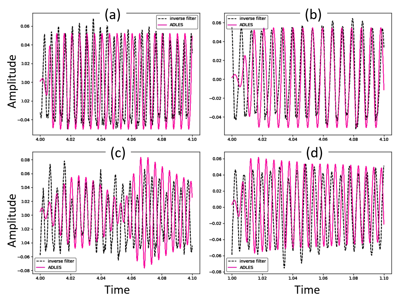
Fig. 3: Glottal flows from inverse filtering and our ADLES estimation for (a) normal speech, (b) neoplasm, (c) phonotrauma, (d) vocal palsy.

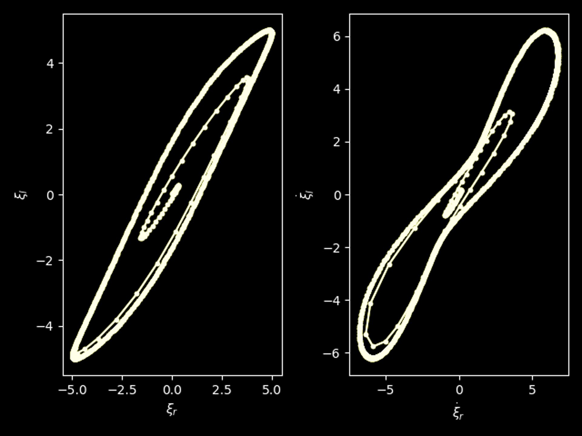
(a)

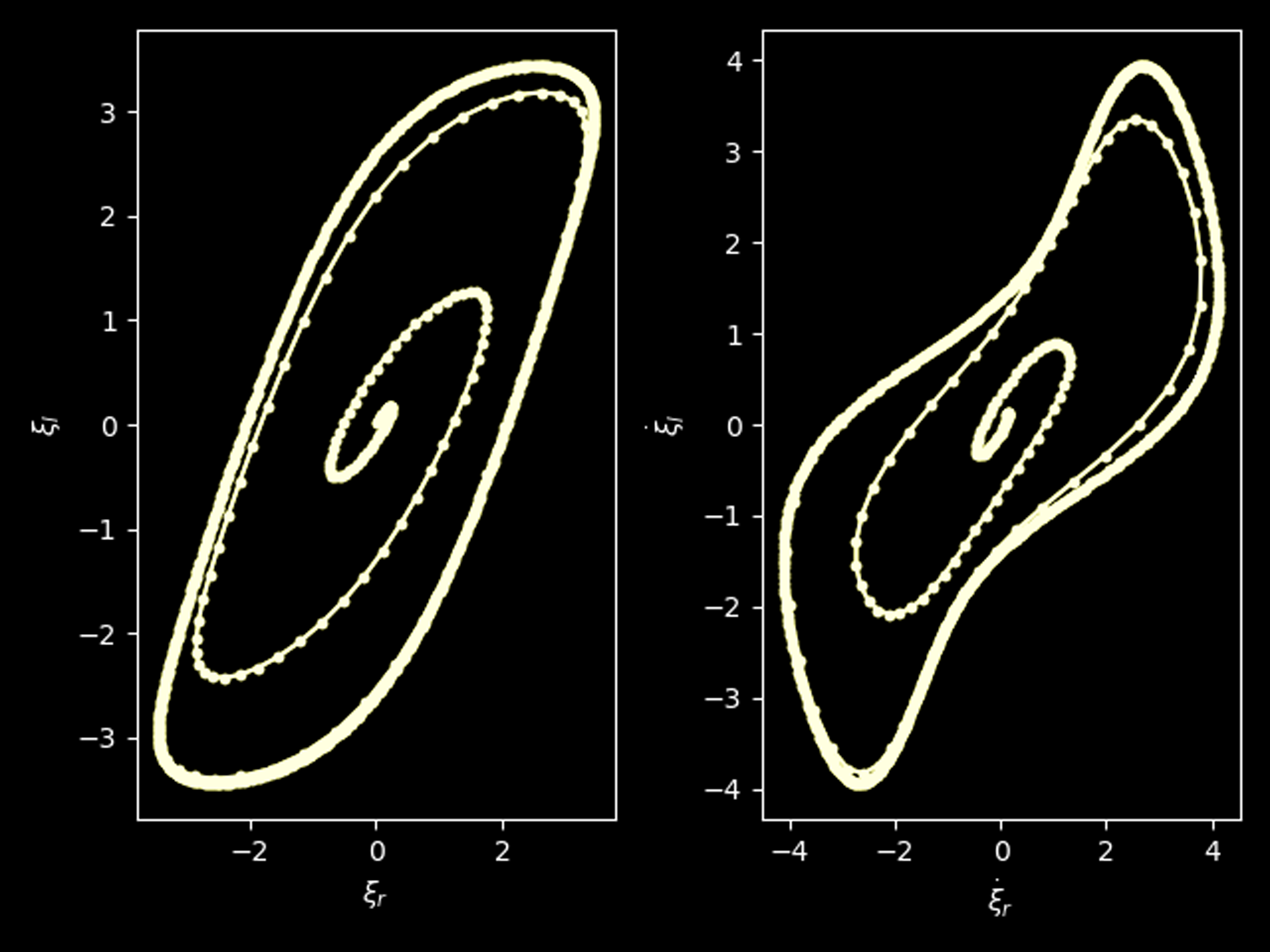
(b)

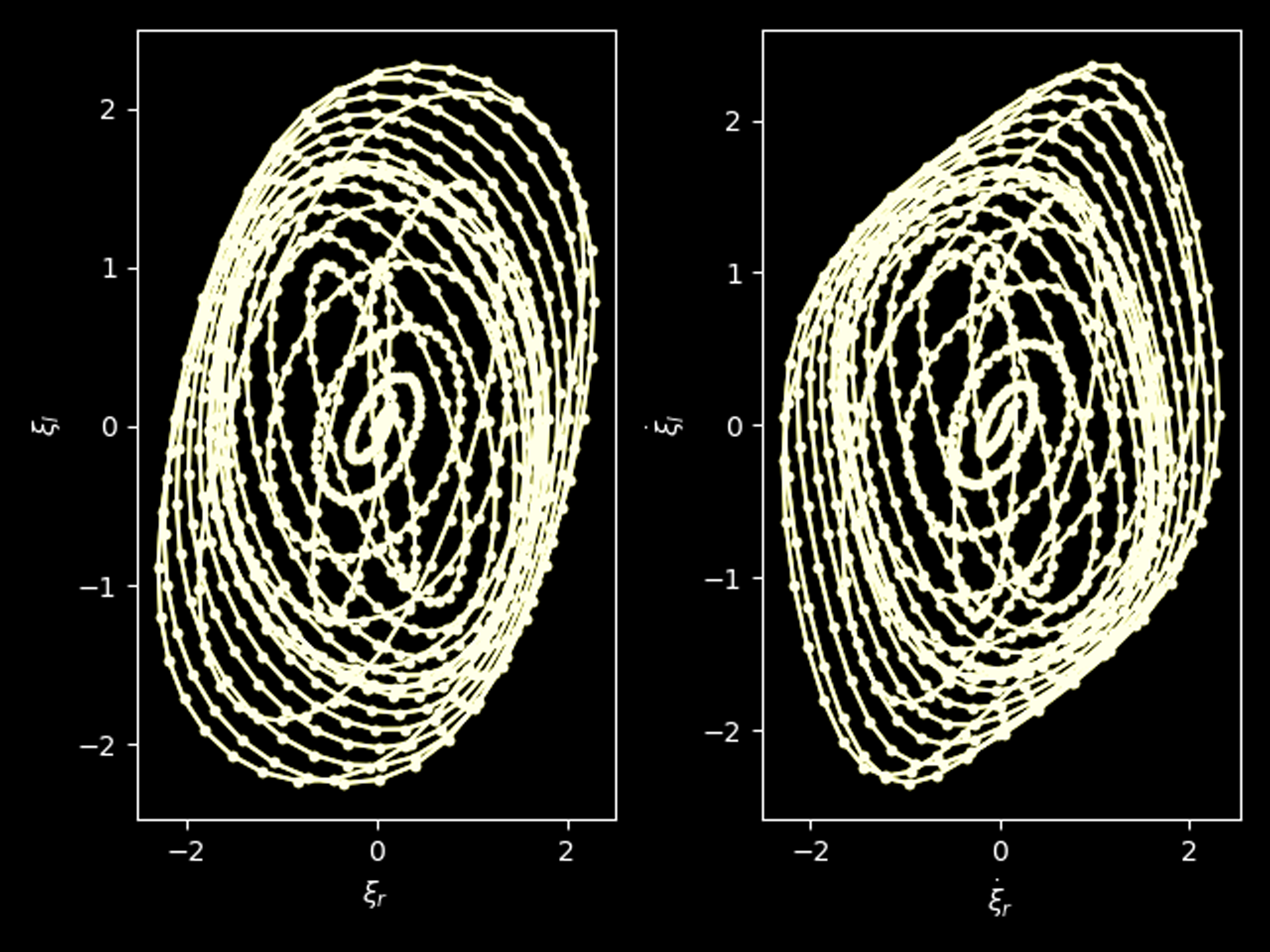
(c)

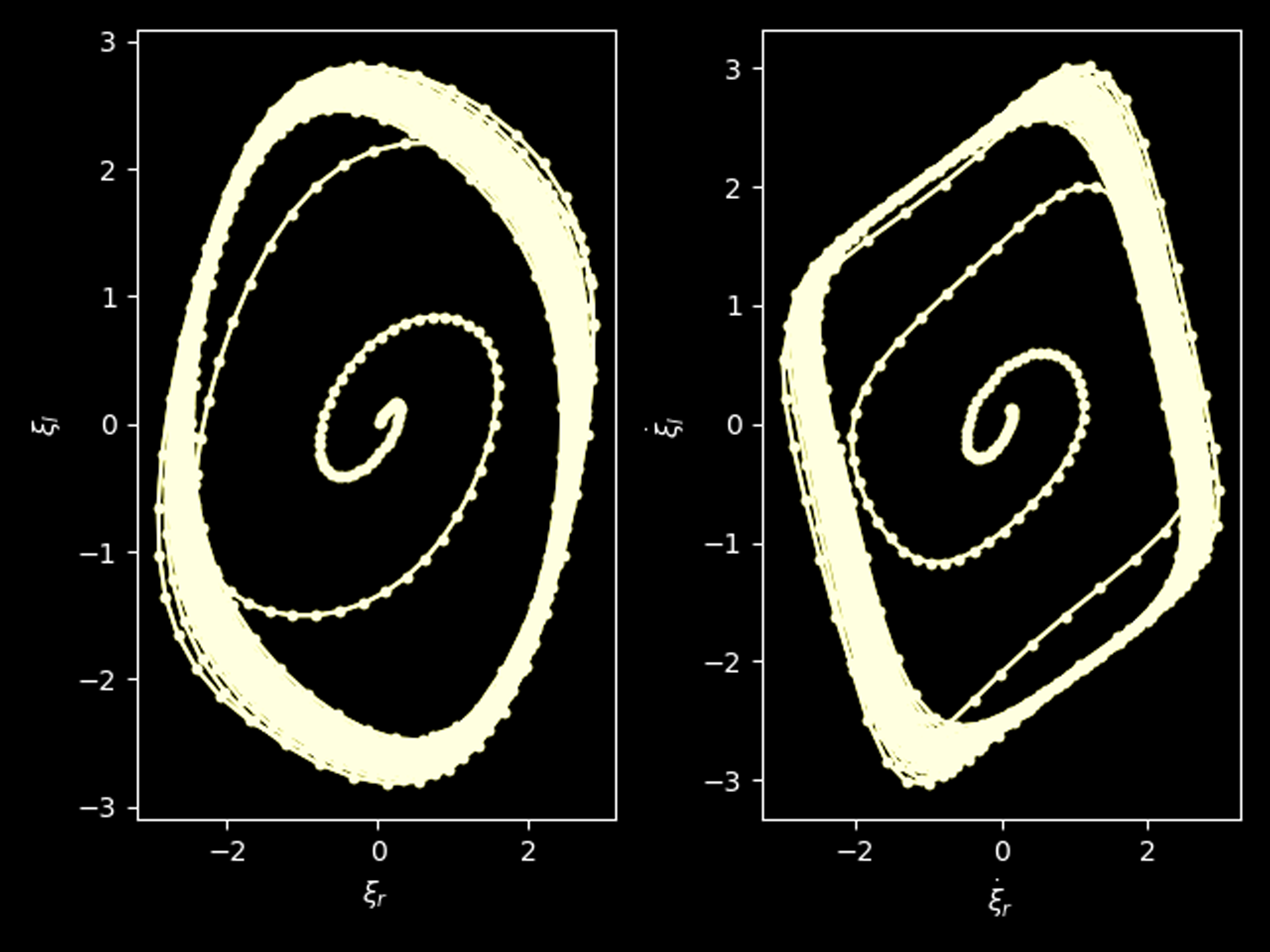
(d)

Fig. 4: Phase portraits of the system from our ADLES estimation for (a) normal speech–1 limit cycle, (b) neoplasm–1 limit cycle, (c) phonotrauma–2 limit cycles, (d) vocal palsy–limit torus. In each panel the left plot shows $\xi_{l}$ vs $\xi_{r}$ and the right plot shows $\dot{\xi}_{l}$ vs $\dot{\xi}_{r}$.

Table 1: Parameters obtained and pathologies identified through ADLES

$\Delta$	$\alpha$	Phase Space Behavior	Pathology	Accuracy
$<0.5$	$>0.25$	1 limit cycle, $1:1$ entr.	Norml.	90%
$\sim 0.6$	$\sim 0.35$	1 limit cycle, $1:1$ entr.	Neopl.	82%
$\sim 0.6$	$\sim 0.3$	2 limit cycles, $1:1$ entr.	Phntr.	95%
$\sim 0.85$	$\sim 0.4$	toroidal, $n:m$ entr.	VclPs.	89%

6 Conclusions

The oscillatory dynamics of vocal folds provides a tool to analyze different phonation phenomena, which in turn characterize different types of voice disorders. In this paper, we have proposed an ADLES method to promote accurate and efficient recovery of the parameters of an asymmetric vocal folds model directly from the speech signal. This allows us to correctly solve for the oscillatory dynamics of the vocal folds for the specific speech signal. But more importantly, the parameters estimated for the model directly allow us, through the bifurcation map, to predict voice pathology. Moreover, the ADLES method significantly alleviates the difficulty of obtaining actual measurements of vocal fold displacements in clinical settings. It can thus be a valuable aid in the diagnosis of different voice pathologies.

References

- [1] Livija Cveticanin, “Review on mathematical and mechanical models of the vocal cord,” Journal of Applied Mathematics, 2012.
- [2] Chitralekha Bhat and Sunil Kumar Kopparapu, “FEMH voice data challenge: Voice disorder detection and classification using acoustic descriptors,” in 2018 IEEE International Conference on Big Data (Big Data). IEEE, 2018, pp. 5233–5237.
- [3] Ina Steinecke and Hanspeter Herzel, “Bifurcations in an asymmetric vocal-fold model,” The Journal of the Acoustical Society of America, vol. 97, no. 3, pp. 1874–1884, 1995.
- [4] James L. Flanagan and Lois Landgraf, “Self-oscillating source for vocal-tract synthesizers,” IEEE Transactions on Audio and Electroacoustics, vol. 16, no. 1, pp. 57–64, 1968.
- [5] Kenzo Ishizaka and James L. Flanagan, “Synthesis of voiced sounds from a two-mass model of the vocal cords,” Bell System Technical Journal, vol. 51, no. 6, pp. 1233–1268, 1972.
- [6] Ingo R. Titze, “The physics of small-amplitude oscillation of the vocal folds,” The Journal of the Acoustical Society of America, vol. 83, no. 4, pp. 1536–1552, 1988.
- [7] Zhaoyan Zhang, Jürgen Neubauer, and David A. Berry, “The influence of subglottal acoustics on laboratory models of phonation,” The Journal of the Acoustical Society of America, vol. 120, no. 3, pp. 1558–1569, 2006.
- [8] Wei Zhao, Cheng Zhang, Steven H. Frankel, and Luc Mongeau, “Computational aeroacoustics of phonation, Part I: Computational methods and sound generation mechanisms,” The Journal of the Acoustical Society of America, vol. 112, no. 5, pp. 2134–2146, 2002.
- [9] Cheng Zhang, Wei Zhao, Steven H. Frankel, and Luc Mongeau, “Computational aeroacoustics of phonation, Part II: Effects of flow parameters and ventricular folds,” The Journal of the Acoustical Society of America, vol. 112, no. 5, pp. 2147–2154, 2002.
- [10] Jorge C. Lucero, “Dynamics of the two-mass model of the vocal folds: Equilibria, bifurcations, and oscillation region,” The Journal of the Acoustical Society of America, vol. 94, no. 6, pp. 3104–3111, 1993.
- [11] Jorge C. Lucero and Jean Schoentgen, “Modeling vocal fold asymmetries with coupled Van der Pol oscillators,” in Proceedings of Meetings on Acoustics ICA2013. ASA, 2013, vol. 19, p. 060165.
- [12] Fariborz Alipour, David A. Berry, and Ingo R. Titze, “A finite-element model of vocal-fold vibration,” The Journal of the Acoustical Society of America, vol. 108, no. 6, pp. 3003–3012, 2000.
- [13] Anxiong Yang, Michael Stingl, David A. Berry, Jörg Lohscheller, Daniel Voigt, Ulrich Eysholdt, and Michael Döllinger, “Computation of physiological human vocal fold parameters by mathematical optimization of a biomechanical model,” The Journal of the Acoustical Society of America, vol. 130, no. 2, pp. 948–964, 2011.
- [14] Brian A. Pickup and Scott L. Thomson, “Influence of asymmetric stiffness on the structural and aerodynamic response of synthetic vocal fold models,” Journal of Biomechanics, vol. 42, no. 14, pp. 2219–2225, 2009.
- [15] Jack J. Jiang, Yu Zhang, and Jennifer Stern, “Modeling of chaotic vibrations in symmetric vocal folds,” Journal of the Acoustical Society of America, vol. 10, no. 4, pp. 2120–2128, 2001.
- [16] Rita Singh, Profiling humans from their voice, Springer, 2019.
- [17] Byron D. Erath and Michael W. Plesniak, “An investigation of jet trajectory in flow through scaled vocal fold models with asymmetric glottal passages,” Experiments in Fluids, vol. 41, no. 5, pp. 735–748, 2006.
- [18] Brad H. Story and Ingo R. Titze, “Voice simulation with a body-cover model of the vocal folds,” The Journal of the Acoustical Society of America, vol. 97, no. 2, pp. 1249–1260, 1995.
- [19] Roger W. Chan and Ingo R. Titze, “Dependence of phonation threshold pressure on vocal tract acoustics and vocal fold tissue mechanics,” The Journal of the Acoustical Society of America, vol. 119, no. 4, pp. 2351–2362, 2006.
- [20] Jorge C. Lucero, Jean Schoentgen, Jessy Haas, Paul Luizard, and Xavier Pelorson, “Self-entrainment of the right and left vocal fold oscillators,” The Journal of the Acoustical Society of America, vol. 137, no. 4, pp. 2036–2046, 2015.
- [21] George David Birkhoff, Dynamical systems, vol. 9, American Mathematical Society, 1927.
- [22] Jack J. Jiang, Yu Zhang, and Jennifer Stern, “Modeling of chaotic vibrations in symmetric vocal folds,” The Journal of the Acoustical Society of America, vol. 110, no. 4, pp. 2120–2128, 2001.
- [23] Jack J. Jiang and Yu Zhang, “Chaotic vibration induced by turbulent noise in a two-mass model of vocal folds,” The Journal of the Acoustical Society of America, vol. 112, no. 5, pp. 2127–2133, 2002.
- [24] Patrick Mergell, Hanspeter Herzel, and Ingo R. Titze, “Irregular vocal-fold vibration—high-speed observation and modeling,” The Journal of the Acoustical Society of America, vol. 108, no. 6, pp. 2996–3002, 2000.
- [25] Chao Tao, Yu Zhang, Daniel G. Hottinger, and Jack J. Jiang, “Asymmetric airflow and vibration induced by the Coandǎ effect in a symmetric model of the vocal folds,” The Journal of the Acoustical Society of America, vol. 122, no. 4, pp. 2270–2278, 2007.
- [26] Victor Isakov, Inverse problems for partial differential equations, vol. 127, Springer, 2006.
- [27] Chao Tao, Yu Zhang, Gonghuan Du, and Jack J. Jiang, “Estimating model parameters by chaos synchronization,” Physical Review E, vol. 69, no. 3, pp. 036204, 2004.
- [28] Yu Zhang, Chao Tao, and Jack J. Jiang, “Parameter estimation of an asymmetric vocal-fold system from glottal area time series using chaos synchronization,” Chaos: An Interdisciplinary Journal of Nonlinear Science, vol. 16, no. 2, pp. 023118, 2006.
- [29] Stefan J. Rupitsch, Jürgen Ilg, Alexander Sutor, Reinhard Lerch, and Michael Döllinger, “Simulation based estimation of dynamic mechanical properties for viscoelastic materials used for vocal fold models,” Journal of Sound and Vibration, vol. 330, no. 18-19, pp. 4447–4459, 2011.
- [30] Chao Tao, Yu Zhang, and Jack J. Jiang, “Extracting physiologically relevant parameters of vocal folds from high-speed video image series,” IEEE Transactions on Biomedical Engineering, vol. 54, no. 5, pp. 794–801, 2007.
- [31] Man Mohan Sondhi, “Model for wave propagation in a lossy vocal tract,” The Journal of the Acoustical Society of America, vol. 55, no. 5, pp. 1070–1075, 1974.
- [32] Paavo Alku, “Glottal inverse filtering analysis of human voice production—a review of estimation and parameterization methods of the glottal excitation and their applications,” Sadhana, vol. 36, no. 5, pp. 623–650, 2011.