The attoclock and the tunnelling time debate

Abstract

Attosecond angular streaking, also known as the “attoclock”, employs a short elliptically polarized laser pulse to tunnel ionize an electron from an atom or a molecule and to put a time stamp on this process by deflecting the photoelectron in the angular spatial direction. This deflection can be used to evaluate the time the tunneling electron spends under the classically inaccessible barrier and to determine whether this time is finite. In this review, we examine the latest experimental and theoretical findings and present a comprehensive set of evidence supporting the zero tunneling time scenario.

• 9 August –

1 Introduction

Time, one of the most elusive concepts in quantum mechanics, has never been under greater scrutiny since a recent development and application of ultrafast pulsed laser techniques. With the temporal resolution down to only a few attoseconds (1 as = $10^{-18}$ s), ultrafast electron dynamics in atoms and molecules can now be probed on its native time scale [RevModPhys.81.163]. This unprecedented experimental capability allows one to test the most fundamental concepts at the heart of quantum mechanics. One such concept is the tunneling time, i.e. the time which a tunneling particle spends under the barrier in a classically inaccessible region.

Experimental access to tunneling time has been opened following the pioneering “attoclock” experiments by Eckle et al (2008a, 2008b) . In these experiments, timing of the tunneling ionization was mapped onto the photoelectron momentum by application of an intense elliptically polarized laser pulse. Such a pulse served both to liberate an initially bound atomic electron and to deflect it in the angular spatial direction. This deflection was taken as a measure of the tunneling time.

The concept of tunneling time has received its first attention soon after the birth of quantum mechanics. 1932PhysRevMacColl considered a sub-barrier transmission of a one-dimensional wave packet and concluded that

“…there is no appreciable delay in the transmission of the packet through the barrier.”

This work triggered an intensive debate and the concept of tunnelling time had been re-examined again under different guises. In a summarizing review, RevModPhys.66.217 made the following remark:

“Over sixty years ago, it was suggested that there is a time associated with the passage of a particle under a tunnelling barrier. The existence of such a time is now well accepted; in fact the time has been measured experimentally. There is no clear consensus, however, about the existence of a simple expression for this time, and the exact nature of that expression …”

It is for this elusive nature of the tunnelling time that the first attoclock experiments by Eckle et al (2008a, 2008b) were so enthusiastically welcomed. The conclusion of these experiments was resolute. Eckle et al (2008a) unequivocally stated that

“Thus, the numerical simulations, like the experiment, lead to a momentum distribution that is consistent with a zero delay time for tunnelling.”

A similar statement was made in the follow-up investigation by the same group [2012NatPhysPfeiffer]:

“The excellent agreement of our theory for both atoms (Ar and He) and over a large intensity range below and above the Keldysh parameter $\gamma=1$ confirms zero tunnelling time within the experimental accuracy of 10 as.”

These early experiments were conducted with relatively high laser field intensities. In more recent experiments [PhysRevLett.111.103003, 2014OpticaLandsman], low field intensities were accessed. As is seen from a schematic representation of an attoclock measurement (Figure 1 a-b), a weaker laser field bends the Coulomb barrier less and hence the tunnel becomes wider in a low field regime. This possible increase of the tunnel width may have resulted in a finite tunnelling time determination in the later refined measurements [2014OpticaLandsman, 2015PhysRepLandsman]. Following a very thorough review and analysis of these experiments, 2019JModOptHofmann concluded that

“…models including finite tunnelling time are consistent with recent experimental measurements”

Thus, the whole decade of the attoclock experiments has ended inconclusively keeping the door open for a finite tunnelling time.

Figure 1: A man-made tunnel: a graphical illustration of the attoclock experiment (a) The laser field $E_{0}$ bends the atomic Coulomb potential and creates a penetrable potential barrier through which an initially bound electron tunnels out. Attoclock measures the time the electron spends under the barrier in a classically inaccessible region. Adapted from 2015PhysRepLandsman. (b) As the laser field decreases to $E_{1}<E_{0}$, the width of the barrier increases and this may increase the tunnelling time. c) A Wigner time visualization by the photoelectron trajectory back-propagation in the multiphoton ionization regime. Adapted from PhysRevLett.105.233002. d) The same trajectory visualization in the tunnelling ionization regime. Data are from 2017PRLCamus.

Fresh fuel to the tunnelling time debate was added by a recent measurement of 2017PRLCamus who titled their work

“Experimental evidence for quantum tunnelling time”.

Not only did they detect a finite tunnelling time, but the values attached to this time were very large, more than 100 as. These values were derived by the Wigner trajectory analysis. Such an analysis is usually conducted to visualize the Wigner time that is characteristic of strong field ionization in the multi-photon regime [M.Schultze06252010, PhysRevLett.105.233002]. The Wigner time [PhysRev.98.145] characterizes the photoelectron group delay, or advancement, relative to the free space propagation. It can be visualized by the back-propagation of the photoelectron trajectory to the origin and its termination at a “time zero” that is displaced relative to the peak electric field of the driving laser pulse. This displacement is the measure of the Wigner time delay. Figure 1c) illustrates the Wigner time determination by back-propagating the photoelectron trajectories emitted from the $2s$ and $2p$ shells of the Ne atom. The inset of this figure clearly shows the origin of these trajectories to be displaced to the opposite directions relative to the peak of the driving pulse. Thus determined Wigner time difference of the $2s$ and $2p$ shells of Ne is of the order of 10 as. While the initial measurement by M.Schultze06252010 valued this difference at $21\pm 5$ as, a more recent experiment by Isingerer7043 found it in a much closer agreement with the theoretical predictions. As is seen from Figure 1(a-b), in the multi-photon ionization regime, the photoelectron has enough energy to make a vertical transition and emerges in the continuum close to the origin. In the tunnelling ionization regime, the photoelectron makes a horizontal transition and the tunnel exit point extends to many Bohr radii away from the origin (Figure 1 d). Termination of the photoelectron trajectory at such a large distance results in a seemingly large “Wigner” tunnelling time running over 100 as. However, such a Wigner-like definition of the tunnelling time is questionable as a classical photoelectron trajectory cannot be continued into a classically inaccessible region under the barrier. Moreover, tunneling acts as an energy filter, favouring higher-energy components of the photoelectron wave packet and distorting the group delay 2019JModOptHofmann.

Meanwhile, contrary to some experimental evidence supporting a finite tunneling time, a growing body of theoretical work points to a vanishingly small or even zero tunnelling time. 2019JModOptHofmann based their claim of a finite tunnelling time on a sole helium measurement [PhysRevLett.111.103003, 2014OpticaLandsman] that deviated strongly from semi-classical modeling assuming instantaneous tunnelling. However, this measurement did also deviate very significantly from fully quantum simulations based on a numerical solution of the time-dependent Schrödinger equation (TDSE) [PhysRevA.89.021402, Scrinzi2014]. These ab initio simulations did not require any assumptions regarding tunnelling time or adiabaticity scenario. Scrinzi2014 termed this disagreement as “a very disquieting”. As a possible source of this disagreement, Rost2019 pointed to an inconsistent field intensity calibration which could affect a self-referencing attoclock measurement.

Another group of theoretical investigations advocating a zero tunnelling time is not directly related to the performed experiment. These numerical simulations, which have no laboratory counterparts and that are termed for this reason a numerical attoclock, consider atomic ionization driven by an ultra-short nearly single-optical-cycle laser pulse. The photoelectron momentum distribution (PMD) in such a field configuration is particularly simple. It can be simulated by various simplified, but more physically transparent, techniques such as an analytic $R$-matrix theory [2015NatPhysTorlina], a classical back-propagation analysis , classical-trajectory Monte Carlo simulations [0953-4075-50-5-055602], a classical Rutherford scattering model [2018PRLBray] and the strong field approximation (SFA) implemented within the saddle point method (SPM) [PhysRevA.99.063428]. By making comparisons with these models, the numerical attoclock firmly points to a vanishing tunnelling time [2015NatPhysTorlina, PhysRevLett.117.023002, 2018PRLBray]. It is shown in these works that a noticeable deviation of the PMD from the simple canonical momentum conservation picture is related to the Coulomb field of the ion remainder. The same conclusion was reached in a joint experimental and theoretical investigation on the atomic hydrogen by 2019NatSainadh who made an upper bound estimate on the tunnelling time not exceeding 1.8 as. Similarly, in the molecular hydrogen, such an estimate is under 10 as [Wei2019]. In a numerical attoclock setup on negative ions, with no Coulomb drag on the photoelectron, the tunnelling time is also vanishing [2019PRADouguet].

This growing body of evidence motivates us to reconsider the question of whether an attoclock measurement can be interpreted in terms of a finite tunnelling time. This question is considered in detail in the following sections of this review article. Our concluding remark is that the window for a non-zero ‘tunnelling time’ in the context of attoclock measurements on simple atomic or molecular targets appears to have essentially closed.

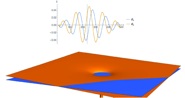
Figure 2: The distortion of the atomic potential $V_{\mathrm{tot}}(\bm{r},t)=1/r+\bm{E}(t)\cdot\bm{r}$ as a function of time for a typical attoclock pulse (orange surface) versus the initial binding energy (blue plane). Where these two surfaces intersect the bound electron is able to adiabatically tunnel. Adapted from Bray2019.

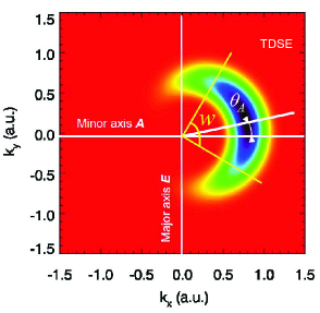
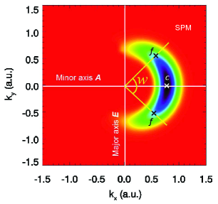
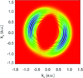
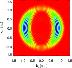
Figure 3: Left column: TDSE calculated PMD of hydrogen for short (top) and long (bottom) pulses. The short pulse is approximately 1.6 fs FWHM at the peak intensity of $\rm{0.86}\times 10^{{14}}~{}W/cm^{2}$, 800 nm, ellipticity $1.0$, and the anti-clockwise helicity. The long pulse is approximately 6 fs FHWM at the peak intensity of $\rm{1.5}\times 10^{{14}}~{}W/cm^{2}$, 770 nm, ellipticity $0.85$, and the clockwise helicity. The PMD is averaged over CEP. Right column: As for left but from a Yukawa potential (screening parameter $a=1$) with the hydrogenic binding energy. The colouration of probability is linear and normalized from red (0.0) to black (1.0). Adapted from PhysRevA.99.063428 (top row) and Bray2019 (bottom row)

2 Attoclock principle

The attoclock employs the rotating electric-field vector $\bm{E}$ of an elliptically polarized laser pulse to deflect tunnel-ionized electrons in the angular spatial direction. The field, that is characterized by the temporal profile $f(t)$, the ellipticity $\epsilon\lesssim 1$ and the magnitude $E_{0}$, is contained in the polarization $(x,y)$ plane:

$$E_{x}(t)={E_{0}f(t)\over\sqrt{1+\epsilon^{2}}}\cos(\omega t+\phi)\ ,\ E_{y}(t)={\epsilon E_{0}f(t)\over\sqrt{1+\epsilon^{2}}}\sin(\omega t+\phi)\ .$$ (1)

The instant of ionization $t_{\rm ion}$ is mapped onto the final momentum vector of the photoelectron at the detector $\bm{p}_{t\to\infty}$. The tunneling ionization is an exponentially suppressed process. Predominantly, it commences at the time $t_{0}$ corresponding to the peak of the driving laser pulse (see Figure 2 for illustration). At this instant, the vector-potential of the driving field $\bm{A}(t_{0})=-\int_{-\infty}^{t_{0}}{\bm{E}(t)}\ dt$ is aligned with the minor $y$ axis of the polarization ellipse . It is expected that the photoelectron emerges from the tunnel with zero velocity (the adiabatic hypothesis) and its kinetic momentum captures the vector potential of the laser field at the time of exit $\bm{p}_{t\to\infty}=-\bm{A}(t_{\rm ion})\ .$ Angular deviation of $\bm{p}_{t\to\infty}$ from the $y$ direction can be simply related to the tunneling time $\theta=\omega\tau$, where $\tau=t_{\rm ion}-t_{0}\$. The Coulomb field of the ion remainder makes this interpretation less straightforward. Nevertheless, the tunneling time can still be determined using a semi-classical trajectory simulation.

Any direct comparison of a fundamentally quantum mechanical process with its classical analogue has many caveats. The attoclock principle illustrates these caveats most vividly. Firstly, the PMD needs to be characteristic of only one or few selected classical trajectories. As was shown by 0953-4075-39-14-R01, for close-to-circular polarization, this number is exceeding by one the number of the driving pulse oscillations. For a pulse with the temporal profile

$$f(t)=\left\{\begin{array}[]{ll}\cos^{4}(\omega t/2N)&-N\pi/\omega<t<+N\pi/\omega\\ 0&\mathrm{elsewhere}\\ \end{array}\right.\ ,$$ (2)

which becomes nearly single-cycle with $N=2$, there are only 3 contributing trajectories of which the one is strongly dominant whereas the other two can be safely neglected. Correspondingly, the fully quantum mechanical simulation and the classical trajectory simulation return very similar PMDs which both have a well defined angle about which they are fully symmetric. See the top row of panels in Figure 3 for the quantum-mechanical TDSE simulation (left) and the semi-classical SPM simulation (right). In contrast, for multi-cycle pulses with $N\simeq 5$, the photoelectron momentum distribution becomes less pronounced. It looses its natural symmetry and acquires above-threshold-ionization (ATI) ring structure from inter-cycle interference, a phenomenon unexplainable by classical physics. Examples of such distributions are shown in the bottom row of Figure 3 for the realistic atomic potential (left) and a short-range Yukawa potential (right).

A further consideration pertinent to the observed attoclock momentum distributions in Figure 3 is the effect of the carrier-envelope phase (CEP) $\phi$ entering Equation (1). For short single-cycle pulses (top row) the peak field strength simply rotates in the plane with varying CEP and accordingly the same occurs for the resulting momentum distribution. However, for the few-cycle pulses with elliptical polarization (bottom row), the direction of the peak field strength only changes subtly with a variation of CEP. In fact, it is only the ellipticity that modulates the field strength significantly enough for the distribution to exhibit the characteristic two-lobes observed in the experiment, and for which none have been performed with stable CEP. Consequently, these ‘long pulse’ distributions are dependent on the precise CEP and need to be accordingly averaged over for comparison with a CEP variable experiment.

3 Attoclock interpretation

The second caveat of relating an attoclock measurement to a classical trajectory is the appropriate boundary condition. This typically depends on the assumption of the adiabaticity of the tunneling process, i.e. whether the photoelectron emerges from the tunnel with the zero (adiabatic) or a non-zero (non-adiabatic) velocity. This adiabaticity scenario, in turn, affects the intensity calibrations that have been in use [hofmann2016non]. In the primary experimental work (Eckle et al 2008a, Pfeifer et al 2012) the comparison was performed against a model known as tunnel ionization in parabolic coordinates with induced dipole and Stark shift (TIPIS). This comparison led to the conclusion of zero tunneling time as there was no discernible difference between experimental measurements and the TIPIS predictions. The latter assumed instantaneous tunneling. In the later work, however, PhysRevLett.111.103003 and 2014OpticaLandsman found quite the opposite, with the observed offset angle being much larger than that predicted by TIPIS, and attributed this difference to a finite tunneling time. This comparison is illustrated in Figure 4. In the left panel of the figure, the two experimental data sets of PhysRevLett.111.103003 are shown which are calibrated on the intensity scale under the adiabatic (red) and non-adiabatic (blue) tunneling scenarios. The two analogous TIPIS calculations are also displayed. While the adiabatic TIPIS simulation (red) is in qualitative agreement with the experiment, the non-adiabatic TIPIS (blue) should be discarded as clearly unphysical. A noticeable difference between the adiabatic TIPIS and the adiabatic experiment is wholly attributed to the tunneling time.

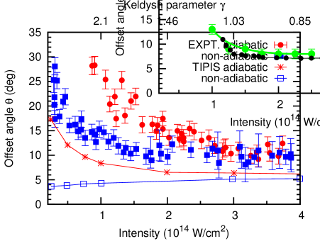
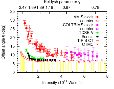
Figure 4: Left: Experimental data and TIPIS simulations from PhysRevLett.111.103003 are shown along with the TDSE calculations by PhysRevA.89.021402 and Scrinzi2014. Right: Experimental data and TIPIS simulations from 2014OpticaLandsman are compared with the same TDSE calculations.

In the same panel, the two TDSE calculations are shown in black [Scrinzi2014] and green [PhysRevA.89.021402]. These TDCS calculations are much closer to the blue non-adiabatic set of experimental data even though the non-adiabatic scenario was discarded in the experiment because of the TIPIS simulation failure. It should be also emphasized that the TDSE simulations were fully ab initio and no specific tunneling scenario was adopted. The only approximation used in both TDSE calculations was the single active electron of the helium atom interacting with the laser field. However, the later and more refined simulation including both active electrons found no electron correlation effects in the He attoclock setting [2017JModOptMajety].

In the right panel of Figure 4, an extended data set of 2014OpticaLandsman is displayed. It contains only the adiabatic data which are shown in red. The experiment is conducted both with the cold target recoil-ion momentum spectroscopy (COLTRIMS, displayed with squares) and a velocity map imaging spectrometer (VMIS, displayed with circles). The experimental data are separated into the clockwise (filled symbols) and the anti-clockwise (open symbols) helicity. The adiabatic TIPIS simulations are carried over with the single trajectory (CT, solid line) and classical trajectory Monte Carlo (CTMC, asterisks) simulation. The shaded area below the CTMC curve is the offset angle admissible under the zero tunneling time scenario. The difference between the experiment and the TIPIS model, which is barely noticeable at large field intensities (COLTRIMS), increases significantly in the low-intensity regime (VMIS). This difference, in principle, could be attributed to a finite tunneling time. However, more likely, it is due to inconsistent intensity calibration. Indeed, the experiment deviates similarly strongly from the ab initio TDSE calculations which do not assume any tunneling hypothesis or adiabaticity scenario.

The latest attoclock measurement that suggested a non-zero tunnelling time was reported by 2017PRLCamus. They adopted theoretical modeling of PhysRevA.90.012116 and evaluated a Wigner trajectory using a fixed-energy propagator calculated from the phase of the solution of the time-independent Schrödinger equation. Such a quasi-stationary approach could only be applied in the strongly adiabatic regime when the energy of the tunneling particle would be conserved. After the quantum Wigner trajectory was found, it was matched at the exit from the tunnel with a classical trajectory with the initial conditions given by the Wigner formalism $p_{\rm exit}=p_{W}$ and $t_{\rm exit}=\tau_{W}$. The latter quantity was adopted as a tunneling time. In addition to a classical trajectory determined by the Wigner initial conditions, 2017PRLCamus defined a so-called simple-man (SM) trajectory in which the photoelectron exits the tunnel instantaneously $t_{\rm exit}=0$ and fully adiabatically $p_{\rm exit}=0$. The Wigner, classical and SM trajectories are exhibited in Figure 1d) for the Kr atom at the field intensity $I=$ $\rm{1.7}\times 10^{{14}}~{}W/cm^{2}$.

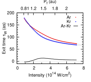
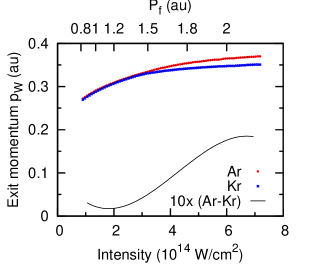
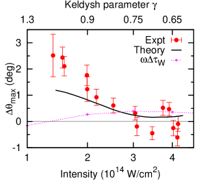
Figure 5: Left and center: the exit time $\tau_{W}$ and the exit momentum $p_{W}$ in Ar (red dots) and Kr (blue dots). Their differences $\Delta\tau_{W}$ and $\times 10\Delta p_{W}$ are shown solid black lines. Right: the experimental observable $\Delta\theta$ and its theoretical estimate, both the original data from 2017PRLCamus, are plotted versus the laser field intensity. The Wigner component $\delta\theta_{W}=\omega\Delta\tau_{W}$ is also shown.

We analyze the results of 2017PRLCamus and the follow up work by Camus2018 in more detail in Figure 5. Neglecting the ionic Coulomb potential in the SM model leads to the final momentum aligned perfectly with the minor polarization axis and having the zero offset angle $\delta\theta=0$. At the same time, for the Wigner trajectory, the additional time delay $\tau_{W}$ manifests itself as a rotation of the asymptotic momentum distribution by $\delta\theta_{\tau}=\omega\tau_{W}$ and the nonzero initial momentum $p_{W}$ to a counter-rotation by $\delta\theta_{p}\approx-p_{W}/p_{E}$ with the drift momentum being $p_{E}=E_{0}/\omega\ .$ Here $E_{0}=\sqrt{I/[I_{0}(1+\epsilon^{2})]}$ while $\epsilon$ is the ellipticity and $I_{0}=$  $\rm{3.51}\times 10^{{16}}~{}W/cm^{2}$ is the atomic unit of the field intensity.

The exit times $\tau_{W}$ and the exit momenta $p_{W}$ for Ar and Kr as functions of the field intensity are exhibited in the left and central panels of Figure 5, respectively. Their differences are calculated from the original data of 2017PRLCamus and also plotted. The right panel displays the final set of the experimental data in which the difference in the attoclock offset angles $\Delta\theta_{\rm max}=\theta^{\rm Ar}_{\rm max}-\theta^{\rm Kr}_{\rm max}$ is compared with the predictions of the theory. Both the theory and experiment are presented by 2017PRLCamus on the momentum scale $\rho^{\rm Ar}(\theta_{\max})=\sqrt{p_{x}^{2}(\theta_{\max})+p_{y}^{2}(\theta_{\max})}\ .$ We assume that $\rho(\theta_{\max})\approx\sqrt{p^{2}_{W}+p^{2}_{E}}$ and place the $\Delta\theta_{\rm max}$ data on the absolute intensity scale using the $p_{W}$ values shown in the central panel of Figure 5. This allows us to plot on the same graph the Wigner time induced component $\Delta\theta^{W}_{\max}=\omega\Delta\tau_{W}$ calculated from the Wigner times difference shown in the left panel. The results are very indicative. The essence of every clock is to tell the time. We observe, however, that the time induced rotation difference is vanishingly small in this experiment. The same can be said about the initial momentum induced component. Indeed, the difference in $p_{W}$ between Ar and Kr is only noticeable at larger intensities. At lower intensities, where $\Delta\theta_{\max}$ is largest, it is induced neither by $\Delta\tau_{W}$ nor $\Delta p_{W}$ but solely by the different effect of the photoelectron scattering in the Coulomb field of the ion reminder. Indeed, as 2017PRLCamus pointed out, the attoclock set up is very sensitive to the tunnel width. This width is estimated in the Keldysh theory as $x_{\rm exit}=I_{p}/E_{0}$ [Keldysh1965]. The difference in the ionization potentials between Ar and Kr causes the difference in $x_{\rm exit}$ which becomes greater in the lower field intensity as $E_{0}$ decreases. This is accompanied by the increase in $\Delta\theta^{W}_{\max}$. Thus, we may say that the attoclock is, in fact, a “nano-ruler” that provides a very accurate determination of $x_{\rm exit}$. It becomes ever more sensitive in the weaker field regime.

4 Hydrogen versus noble gas atoms

Some uncertainty in interpretation of the attoclock measurements on helium [PhysRevLett.111.103003, 2014OpticaLandsman] and heavier noble gas atoms [2017PRLCamus] could possibly be attributed to the effect of many-electron correlation. Indeed, the initial theoretical modeling [PhysRevA.89.021402, Scrinzi2014], which was found at variance with the helium experiment, was conducted in the single active electron approximation while the effect of correlation was neglected. Such a correlation could, in principle, slow down the tunneling process. The tunneling electron may need the time to negotiate with its many-electron environment the fine detail of the tunneling process. However, in the case of He, this was explicitly shown not to be the case [2017JModOptMajety]. Indeed, the remaining electron in the He⁺ ion is so tightly bound that it hardly interacts with the tunneling electron other than by screening the charge of the bare nucleus. This situation may differ for such complex atoms as Ar and Kr where a precise theoretical modeling with an accurate account for many-electron correlation is not feasible at present.

The hydrogen atom is naturally correlation free. Hence, an attoclock measurement on this atom would give the cleanest determination of the tunneling time. However, until very recently, such a measurement was not possible because of a very low density of atomic hydrogen targets and hence a low count rate in the COLTRIMS setting. Finally, this experimental hurdle was overcome and the first hydrogen attoclock experiment was reported by 2019NatSainadh.

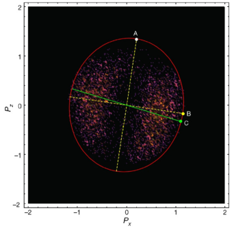
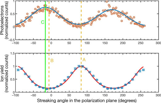
Figure 6: Left: PMD of the hydrogen atom is projected on the polarization plane. Points A and B mark the direction of the major and minor axes of the polarization ellipse. Right: radially integrated counts of the photoelectrons (top) and the photo-ions (bottom). Point C marks the angular maximum of the photoelectrons count. Adapted from 2019NatSainadh

Experimental results of 2019NatSainadh are illustrated in Figure 6. The left panel displays the photoelectron momentum distribution projected onto the polarization plane. The major A and minor B axes of the polarization ellipse are aligned with the electric field $\bm{E}_{0}$ and the vector potential $\bm{A}_{0}$ at the instant of the tunneling. In the SM picture, under the conditions of $\tau_{\rm exit}=0,p_{\rm exit}=0$ and neglecting the Coulomb field of the ion remainder, the PMD should peak in the B direction. However, this peak is displaced. This displacement, taken as the attoclock offset angle $\theta_{A}$, is clearly seen in the right panel of the figure. Here the radially integrated counts of the photoelectrons (top) and the photo-ions (bottom) are shown. The ion counts are obtained with the linearly polarized light, a precursor of the elliptical light, to mark most accurately the major polarization axis direction.

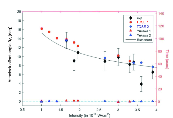
Figure 7: The attoclock offset angle $\theta_{A}$ as a function of the laser pulse intensity is extracted from the experiment and calculated by two TDSE1 and TDSE2 codes. Analogous calculations with a model Yukawa atom are marked as Yukawa 1 and 2. The intensity scaling $I^{-1/2}$ as prescribed by the classical Rutherford scattering model [2018PRLBray] is also marked. Adapted from 2019NatSainadh

The attoclock offset angles $\theta_{A}$ as a function of the laser field intensity are plotted in Figure 7. The experimental values are extracted from the radially integrated photoelectron momentum density projected onto the polarization plane (see Figure 6 for illustration). In the same Figure 7, results of the two calcualtions are also shown. These calculations, marked as TDSE1 and TDSE2, utilized two computer codes developed independently by PhysRevA.93.033402 and PhysRevA.90.013418. To make the closest possible comparison with the experiment, the calculated PMDs were processed in exactly the same way as the experimental data. They were projected on the polarization plane and radially integrated by the same numerical algorithm. As the CEP was not stabilized in the experiment, the calculated data were also averaged over CEP values ranging from 0 to $2\pi$ in steps of $\pi/4$. This procedure led to a rather satisfactory agreement between theory and experiment which validated the experimental technique and the two numerical TDSE solutions.

To eluscidate the long-range Coulomb field effect, a model Yukawa atom was constructed with a screened Coulomb potential $U_{Y}(x)=-Z/re^{-r/a}$ with $a=1$ and $Z=1.908$. The binding energy in such a potential is the same as in the hydrogen atom. The simulated PMDs in the polarization plane are shown in the bottom row of panels in Figure 3 (hydrogen - left, Yukawa - right). In these simulations, the experimental laser pulse parameters are adopted with the FHWM of approximately 6 fs, the peak intensity $\rm{1.5}\times 10^{{14}}~{}W/cm^{2}$, the wavelength of 770 nm and the ellipticity $0.85$ as in 2019NatSainadh. The offset of the peak PMD relative to the minor polarization axis, clearly seen in the hydrogen atom, all but disappears for its Yukawa counterpart. The TDSE 1 and 2 calculations with the Yukawa potential, marked as Yukawa 1 and 2 in Figure 7, produce vanishingly small angular offsets at all laser pulse intensities. The error bars in these Yukawa calculations, resulting from a Gaussian fit to the radially integrated angular distributions, are not exceeding $\delta\theta_{\rm Yukawa}=0.25^{\circ}$ which corresponds to a maximum possible time delay of $\tau_{\rm Yukawa}=\delta\theta_{\rm Yukawa}/\omega=1.8$ as. 2019NatSainadh has taken this number as the upper bound of the tunneling time in hydrogen. Indeed, as the binding energy and hence the tunnel width are identical in the hydrogen and Yukawa atoms, their tunneling times should be also close.

5 Numerical attoclock

Prior to the experiment of 2019NatSainadh, several attempts have been made to evaluate the tunneling time in the hydrogen atom by conducting simulations with ultra-short, nearly single-oscillation pulses. As we outlined in the introduction, these “numerical attoclock experiments”, which could not be matched by laboratory measurements, have a great utility of a very transparent physical interpretation provided by several simplified analytical or numerical tools calibrated against ab initio TDSE solutions. In the following sections, we give a brief review of these tools.

5.1 Analytical $R$-matrix theory

In an analytical $R$-matrix theory (ARM), the probability of detecting an electron with a certain momentum is described by a time integral over all possible instances of ionization [PhysRevA.86.043408]. This integral is expressed in terms of quantum trajectories whose contribution is evaluated using the saddle-point method. The saddle point equations return the starting times of the photoelectron trajectories which turn out to be complex [MIvanov2005]. Their real part is taken as the ionization time and it is counted relative to the peak of the driving laser pulse. The ionization time corresponding to detection of a photoelectron with a momentum $p$ at an angle $\phi$ in the polarization plane is expressed as

$$t_{i}(p,\phi)\equiv{\rm Re}t_{s}(p,\phi)={\phi\over\omega}+\Delta t^{\rm env}_{i}(p,\phi)+\Delta t_{i}^{C}\ \ ,\ \ \Delta t_{i}^{C}=-{dW_{C}(\phi,p)\over I_{p}}$$ (3)

Here $W_{C}$ is the phase acquired by the laser-driven electron due to its interaction with the ionic core and $I_{p}$ is the ionization potential. A small correction $\Delta t^{\rm env}_{i}$ is due to the ultrashort pulse envelope.

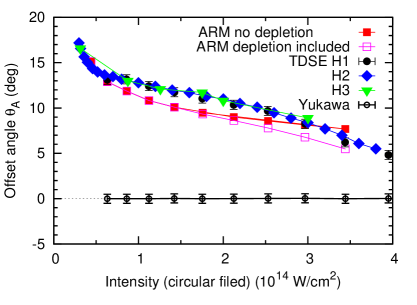
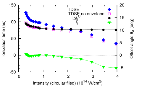
Figure 8: Left: the attoclock offset angles $\theta_{A}$ from the analytical ARM (with and without account for depletion) and numerical TDSE (H1, H2, H3) calculations on the hydrogen atom. A TDSE calculation on the model Yukawa atom is also shown. Right: TDSE H2 calculation is converted to the tunneling time with and without envelope correction. The Coulomb correction $|\Delta t_{i}^{C}|$ is shown separately and subtracted from the envelope corrected TDSE to give the net tunneling time $t_{i}$. The data are from 2015NatPhysTorlina

2015NatPhysTorlina calibrated the ARM against numerically exact TDSE solutions. The TDSE solution for the hydrogen atom can be found exactly within the standard nonrelativistic and dipole approximations. The ARM calibration is illustrated in the left panel of Figure 8 where the attoclock offset angles $\theta_{A}$ are plotted for various laser pulse intensities. The figure displays two sets of the ARM results. The depletion of the target atom is included in one set and its effect becomes noticeable at larger field intensities. The comparison is also made with three sets of TDSE calculations utilizing independently developed computer codes [Muller1999, Tao2012, PhysRevA.89.021402]. Agreement between the TDSE results is very close and it can be used to benchmark the ARM calculations. After the numerical accuracy of the ARM is established, it can be used for extracting the ionization times. For this purpose, Equation (3) is solved for the $p,\phi$ values corresponding to the peak PMDs obtained from TDSE calculations (see the bottom left panel of Figure 3 as an example). The ionization times extracted from the ARM and TDSE calculations are plotted in the right panel of Figure 8. Here the TDSE H2 offset angles are converted to the ionization times using the first term in Equation (3). By adding the second term, an envelope-free TDSE result is obtained. When both the envelope correction and the Coulomb correction $|\Delta t_{i}^{C}|$ ( shown separately in the figure) are subtracted, the ionization times become very small. They deviate noticeably from zero at larger field intensities when the depletion effect becomes strong. This deviation to negative ionization times mean that those photoelectrons arrive to the detector that started tunneling before the laser pulse reached its peak value. When this peak value is reached, the target atom is already depleted. This observation challenges one of the core assumptions of the attoclock measurement. Based on the exponential sensitivity of strong-field ionization to the electric field, it is assumed that the highest probability for the electron to tunnel is at the peak of the electric field. It turns out that this assumption is not always correct. Meanwhile, under no condition is the ionization time positive, i.e. traversing the potential barrier does not take any real time.

5.2 Classical back-propagation

Ni and co-authors [PhysRevLett.117.023002, PhysRevA.97.013426] proposed a novel computational scheme which allowed them to determine the time and position of the electron exiting the tunnel in strong field atomic ionization. The scheme involves a quantum propagation of the ionized electron for a sufficiently long time and its return, by back-propagation, to the point of exit along various classical trajectories. Only those trajectories are accepted that pass near the origin with close to zero velocities, i.e. if the kinetic momentum in the instantaneous field direction vanishes. Typically this condition is fulfilled several times along a trajectory, and the event closest to the ion is identified as the tunnel exit. The ensemble of the tunneling ionization trajectories determines a distribution of the tunneling times ${\mathcal{P}}(\tau)$ relative to the peak position of the driving laser pulse. The mean tunneling time and the total tunneling probability are calculated as $\langle\tau\rangle=\int d\tau\tau d{\mathcal{P}}/d\tau$ and $P_{\rm tun}=\int d\tau{\mathcal{P}}(\tau)\ ,$ respectively. Meanwhile, the quantum propagation of the photoelectron wave function for a sufficiently long time allows one to find the total ionization probability $P_{\rm ion}=\int|\Psi|^{2}d\bm{r}$. By knowing both $P_{\rm ion}$ and $P_{\rm tun}$, the fraction of not-tunneling ionization events can be expressed as $\chi=(P_{\rm ion}-P_{\rm tun})/P_{\rm ion}\ .$

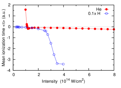
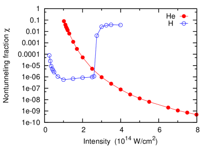
Figure 9: Left: The mean ionization time $\langle\tau\rangle$ in He and H atoms as a function of the laser field intensity. Right: The fraction of non-tunneling ionization events $\chi$ in He and H across the same field intensity range. The data are from PhysRevLett.117.023002

Results of the tunneling time determination for hydrogen and helium atoms are shown in the left panel of Figure 9. The mean tunneling time $\langle\tau\rangle$ is close to zero for both target atoms when the fraction of non-tunneling ionization events is small. This fraction grows for both targets at the edges of the considered laser pulse intensity range. In helium, because of its larger ionization potential, this fraction becomes significant in the low-intensity range at the onset of the multi-photon ionization regime. We note that $\gamma=2$ for He at $I=$ $\rm{1}\times 10^{{14}}~{}W/cm^{2}$. The same increase in $\chi$ is seen at low intensities for H as well, however, it is not that strong and not exceeding $10^{-4}$. At the same time, because of a lower ionization potential, the depletion effect is much stronger for H and it affects the fraction of non-tunneling ionization events at the higher intensity range. Here the mean tunneling time becomes strongly negative. The same effect was observed by 2015NatPhysTorlina and can be seen in Figure 8. When the tunneling ionization is the dominant mechanism, in both atoms the mean tunneling time $\langle\tau\rangle\simeq 0$.

5.3 Classical photoelectron scattering

A significant increase of the attoclock offset angle in the low-intensity regime can be attributed to a thicker potential barrier, as is illustrated in Figure 1b). At the same time, a weaker field drives the photoelectron to the detector slower, thus subjecting it to a prolonged action of the Coulomb force. To disentangle these two competing processes, 2018PRLBray devised a model in which the classical scattering of the photoelectron in the Coulomb potential is considered. The scattering angle in the attractive potential $V(r)=-Z/r$ is given by the Rutherford formula [Landau1982].

$$\tan{\theta\over 2}={1\over v_{\infty}^{2}}{Z\over\rho}\ \ ,\ \ \rho={I_{p}\over E_{0}}\ \ ,\ \ v_{\infty}=A_{0}={E_{0}\over\omega}\ .$$ (4)

The distance of the closest approach $\rho$ in this expression is equated in this model with the Keldysh tunnel width expressed via the ionization potential $I_{p}$ and the maximum field strength $E_{0}$. The photoelectron velocity at the detector $v_{\infty}$ is determined by the peak value of the vector potential. With these assumptions, the attoclock offset angle in the case of the pure Coulomb potential takes the form

$$\theta_{A}=\frac{1}{2}\theta\simeq{\omega^{2}\over E_{0}^{2}}{Z\over\rho}={\omega^{2}\over E_{0}}{Z\over I_{p}}\ .$$ (5)

In the above expression, the action of the laser field during the photoelectron propagation to the detector is neglected. This assumption is only valid for very short and weak laser pulses. The key feature of the KR model is its intensity dependence $I^{-1/2}$ which explains the growth of the attoclock angle $\theta_{A}$ in the low field regime due to a greater elastic scattering of a slower photoelectron in the Coulomb field. This field dependence is drawn in Figure 7.

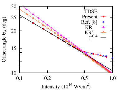
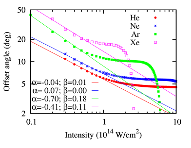
Figure 10: Left: The attoclock offset angle $\theta_{A}$ of the hydrogen atom driven by a single-oscillation lather pulse. The results of the TDSE calculations of 2018PRLBray and 2015NatPhysTorlina are displayed. A comparison with the prediction of the KR model is made. Right: the attoclock offset angles $\theta_{A}$ of noble gas atoms driven by a single-oscillation lather pulse. The CTMC calculation by 0953-4075-50-5-055602 is fitted with a generalized KR ansatz Adapted from 2018PRLBray

Thus defined Keldysh-Rutherford (KR) model was validated in the numerical attoclock settings on hydrogen against numerical TDSE calculations with a single oscillation laser pulse. Results of this validation are shown in the left panel of Figure 10. Here TDSE calculations of 2018PRLBray and the H2 set of 2015NatPhysTorlina are shown to be nearly indistinguishable. This is compared with the two KR and KR^′ estimates. The KR refers to Equation (5), whereas the KR^′ does not make the small angle approximation for the tangent function. The KR scales at all intensities as $I^{-0.5}$ by construction. Fitting the KR$′$ in the low intensity range yields $I^{-0.44}$. The TDSE results display a similar dependency $I^{-0.41}$ for the same region but then flatten and deviate from both the KR and KR$′$. This is understandable as the KR model is expected to work for weak fields only when the field-driven trajectory is close to that involved in the field-free scattering. Within the range of its validity, the KR model attributes nearly all of the attoclock offset angle $\theta_{A}$ to the Coulomb scattering.

Although the KR model is developed explicitly for hydrogenic targets, it can be also applied to other atoms. Indeed, the asymptotic charge affecting the departing photoelectron is always the same $Z=1$ for all neutral atomic targets. So the basic premise of the KR model remains valid. To test this model for other atoms, an extended set of numerical attoclock simulations [0953-4075-50-5-055602] was chosen. These simulations are conducted using the CTMC method. In the right panel of Figure 10, the CTMC offset angles are fitted with a generalized KR ansatz

$$\theta_{A}(I)=\frac{\omega^{2}}{I_{p}}\frac{(1+\alpha)}{(I/2I_{0})^{0.5+\beta}}\ ,$$ (6)

where $I_{0}=$ $\rm{3.51}\times 10^{{16}}~{}W/cm^{2}$ is one atomic unit of field intensity. Parameters $\alpha$ and $\beta$ indicate the deviation of the CTMC calculation from the KR predictions. For small intensities, the scaling of the offset angles with the field intensity is indeed close to $I^{-0.5}$. There is strongest deviation from the KR prediction in Ar and Xe where the fitting parameters are comparatively large. At the same time, these parameters are close to zero for the targets with the larger ionization potentials, He and Ne.

5.4 Strong field approximation

While the KR model neglects entirely the driving of the photoelectron by the laser pulse beyond the tunnel exit, the strong field approximation (SFA) neglects completely the Coulomb field of the ion remainder. Under the latter assumption, the photoelectron motion can be traced along a few dominant trajectories by the time integration of the quasi-classical action. This integration can be carried over by the steepest descent technique using the saddle point method (SPM) (Miloŝević et al 2002, 2006) . This approach is justified when the electron action accumulated along a quasi-classical trajectory is large, $S\gg\hbar$. This is usually the case in strong low-frequency laser fields.

The ionization amplitude in the SFA is written as (Miloŝević et al 2002, 2006)

$$D({\bm{k}}) = -i\sum_{s=1}^{N_{\rm SP}}\left\{2\pi i\over{\bm{E}}(t_{s})\cdot[{\bm{k}}+\bm{A}(t_{s})]\right\}^{1/2}\langle{\bm{k}}+\bm{A}(t_{s})|\bm{r}\cdot{\bm{E}}(t_{s})|\psi_{0}\rangle\ \exp[iS_{{\bm{k}}}(t_{s})]\ ,$$ (7)

where $S_{\bm{k}}(t)=\int^{t}dt^{\prime}\{[{\bm{k}}+A(t^{\prime})]^{2}/2+I_{p}\}$ is the semi-classical action. The summation in Equation (7) is carried over $N_{\rm SP}$ saddle points $t_{s}$ that are solutions of the saddle point equation

$$\partial S_{{\bm{k}}}(t_{s})/\partial t=[{\bm{k}}+\bm{A}(t_{s})]^{2}/2+I_{p}=0\ .$$ (8)

For circular polarization, the number of the saddle points $N_{\rm SP}=N+1$, where $N$ is the number of the pulse oscillations [0953-4075-39-14-R01]. With the presently chosen envelope (2) with $N=2$, $N_{\rm SP}=3$ of which only one dominant SP makes the overwhelming contribution to the PMD shown on the bottom right panel of Figure 3.

The main difference between the PMDs shown on the left and right bottom panels of Figure 3 is that $\theta_{A}=0$ in the SFA with SPM. This has long been a well-known fact, see e.g. 0953-4075-42-16-161001. This fact serves as another indication of the main contribution to the attoclock offset angle coming from the Coulomb field of the residual ion. This field is neglected in the SFA. Except for the vanishing offset angle, the overall structure of the PMD in the polarization plane is reproduced remarkably well by the SPM. This PMD can be quantified by its angular width $\cal W$. This width is marked on the top panels of Figure 3 between the fringes of the PMD ($f$-points) while the center of this distribution is marked with the $c$-points. Numerically, the width $\cal W$ is extracted from the Gaussian fitting to the radially integrated momentum density. The width parameter ${\cal W}(I)$ extracted from the TDSE and SPM calculations are shown on the left panel of Figure 11 as functions of the field intensity $I$. This dependence is not monotonous which can be qualitatively understood from the SFA formulas given by Mur2001 for a continuous elliptical field. In this case, the SP equation (8) can be solved analytically. For strong fields, when the Keldysh adiabaticity parameter $\gamma\ll 1$, the angular width grows with intensity. In the opposite limit $\gamma\gg 1$ the width is falling with intensity. The minimum between these falling and rising intensity dependence of the width occurs around $\gamma\simeq 1$.

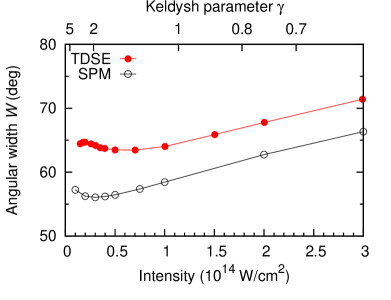
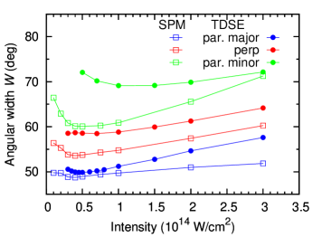
Figure 11: Left: Angular width ${\cal W}(I)$ of the PMD in the polarization plane as a function of the field intensity $I$ for the atomic (left) and molecular (right) hydrogen. The TDSE and PMD calculations are shown. The H₂ molecule is aligned perpendicular to the polarization plane (red), parallel to the major polarization axis $\hat{\bm{e}}_{y}$ (black) and parallel to the minor polarization axis $\hat{\bm{e}}_{x}$ (green). Adapted from PhysRevA.99.063428

The SPM technique can be easily adapted to the H₂ molecule. In this case, the SPM equation (7) acquires an additional term $(-1)^{j}{\bm{E}}(t_{sj})\cdot{\bm{R}}/2\ .$ This term defines the energy gain or loss for the electron to travel to the molecule midpoint and has the opposite signs for different atomic sites $j=1,2$. Accordingly, the single dominant SP in the atomic case is split into two points. The corresponding factor $\exp[\pm i{\bm{k}}\cdot{\bm{R}}/2]$ in the ionization amplitude defines the phase difference between the two wave packets emitted from different atomic sites. The molecular terms in both the SPM and the ionization amplitude vanishes when the molecule is aligned perpendicular to the polarization plane while ${\bm{E}}$ and ${\bm{k}}$ are bound to this plane and hence the two solutions $t_{s1}$ and $t_{s2}$ become identical.

The effect of the molecular orientation is illustrated in the right panel of Figure 11 where the angular width parameter $\cal W$ for the H₂ molecule is displayed in three orientations: perpendicular to the polarization plane (shown with red symbols), aligned with the peak ${\bm{E}}_{0}$ field (“major” axis, blue symbols) and with the peak $\bm{A}_{0}$ potential (“minor” axis, green symbols). Both the TDSE and SPM results are shown (filled circles and open squares, respectively). The angular width $\cal W$ varies very significantly depending on the molecular orientation. Qualitatively, this behaviour is similar in the TDSE and SPM calculations. The latter model allows for the understanding of this behavior qualitatively in terms of the two-center interference. For a given in-plane orientation the interference term effectively increases (decreases) the ionization potential thus increasing (or decreasing) the Im $t_{s}$ and relative contribution of the corresponding saddle points.

6 Improved attoclock

When the tunneling ionization is induced by a long circularly polarized laser pulse, the PMD in the polarization plane becomes a circle. However, if a weak linearly polarized field is superimposed, the maximum of the laser field is attained when the two fields are in phase. Because of an exponential sensitivity of the tunneling ionization, such a superposition produces a pronounced peak in the PMD which can be easily traced, both experimentally and numerically.

Such an “improved attoclock” experiment was conducted in the laboratory and modeled theoretically by PhysRevLett.123.073201. They combined a circularly polarized pulse of 25 fs at 800 nm and $\rm{1.1}\times 10^{{14}}~{}W/cm^{2}$ with a linearly polarized second harmonic at 400 nm and $\rm{6}\times 10^{{12}}~{}W/cm^{2}$. The phase between the two-color fields was precisely monitored. The photoelectron momentum distribution of the argon atom was measured using the COLTRIMS technique. When the 800 nm field made a cycle, the two field vectors overlapped once along the direction of the $z$ axis, and at this instant, the electric field strength reached the maximum ${\bm{E}}_{0}$. Accordingly, the $x$ axis, the direction of the maximum vector potential $\bm{A}_{0}$, served as the attoclock hand. The displacement of the PMD peak relative to the attoclock hand was observed experimentally and simulated numerically under several different approximations.

In the crudest SFA simulation, the transition matrix element was numerically integrated and the angle of the most probable momentum was obtained strictly along the attoclock hand in the $-x$ direction, as expected. In a more advanced TDSE simulation with an effective potential

$$V_{\rm eff}=−[1+(Z-1)e^{-r/r_{s}}]r\ ,$$ (9)

constructed to match the ionization potential of the Ar ($Z=18$) atom, the most probable momentum pointed away from the attoclock hand towards the experimentally observed maximum.

Furthermore, the SFA wave function $\psi$ was used to construct the Wigner function

$$W(v,r;t)=\pi^{-1}\int dv^{\prime}\psi^{*}(v+v^{\prime},t)e^{-2irv^{\prime}}\psi(v-v^{\prime},t)\ .$$ (10)

The latter was employed to determine the most probable momentum and the time at the tunnel exit $x_{\rm exit}=I_{p}/E_{0}$. Thus defined exit time and momentum were tested under the experimental conditions of 2017PRLCamus and found to be very similar with the original values. Having conducted this test, PhysRevLett.123.073201 simulated their measurement and obtained a quite significant longitudinal exit momentum of 0.4 au and an exit time over 200 as. They used these values as initial conditions in their CTMC simulations. The latter were conducted both with and without considering the Coulomb potential in the Newtonian equation of motion. When considering the Coulomb potential, the simulation using the Wigner initial conditions reproduced the results of the experiment and the TDSE. Without this potential, the PMD peaked strictly in the attoclock hand direction without any visible offset.

These results confirm the conclusion that we have already reached in this review several times. The offset angle of the attoclock, both in its original or an improved configuration, is attributed wholly to the effect of the Coulomb field of the ion reminder. The Wigner time, no matter how large it could be, is rather meaningless. It has nothing to do with the angular reading of the attoclock which is not, in fact, a clock but rather a very precise “nano-ruler”.

7 Conclusion and outlook

We reviewed recent results related to attoclock measurements and calculations on various atomic and molecular targets. Our main emphasis was on the determination of the tunneling time, i.e. the time the tunneling electron spends under the classically inaccessible barrier. This interval of time is measured between the peak of the electric field, when the bound electron starts tunneling, and the instance the photoelectrin exits the tunnel. At this instance, the photoelectron momentum captures the vector potential of the driving laser pulse. In the experiment, the tunneling time is extracted from the offset angle between the angular maximum of the photoelectron momentum distribution in the polarization plane and the attoclock hand. This hand points along the vector potential direction $\bm{A}_{0}$ at the instant of tunneling ionization when the electric field of the laser pulse ${\bm{E}}_{0}$ is at its peak value. An alternative explanation of this angular offset is due to the photoelectron scattering in the Coulomb field of the ion remainder. Various arguments are presented here in support of the latter interpretation. Firstly, the offset angle vanishes when the Coulomb potential is substituted with its short-range Yukawa counterpart. The offset angle in the Yukawa atom and the Yukawa molecule are as small as $0.25^{\circ}$ [2019NatSainadh] and $2^{\circ}$ [Wei2019], respectively. Similarly, the offset angle is absent in negative ions [2019PRADouguet]. Second, the offset angle is missing entirely in the strong field approximation when the Coulomb field is neglected [0953-4075-42-16-161001, PhysRevA.99.063428]. Lastly, nearly all of the rapid growth of the offset angle in the low laser field regime is attributed to the Coulomb potential [2018PRLBray]. A gap between the naked Coulomb and a hard screened Yukawa potentials can be spanned continuously by varying the screening length.

Several numerical attoclock simulations with a short, nearly single-oscillation laser pulse, return specific estimates of the tunneling time [2015NatPhysTorlina, PhysRevLett.117.023002, PhysRevA.97.013426]. In the absence of the target atom depletion and well in the tunneling ionization regime $\gamma<1$, this time is close to zero. The depletion effect may cause the effective tunneling time to be negative, i.e. the tunneling process starts before the electric field of the driving pulse reaches its maximum. When the electric field is at its peak, there are no bound electrons left in the target atom to tunnel. Meanwhile, the effective tunneling time is never positive, i.e. there is no delay in the tunneling process which is therefore instantaneous.

There are two experimental observations which could be interpreted in terms of a finite tunneling time. The helium atom measurement in the low field regime [PhysRevLett.111.103003, 2014OpticaLandsman] returned very large offset angles which were at variance with the semi-classical modeling assuming instantaneous tunneling. This measurement was also in strong disagreement with fully ab initio calculations [PhysRevA.89.021402, Scrinzi2014] in which no assumptions on the tunneling scenario was assumed. The relative Ar versus Kr measurement by 2017PRLCamus returned an intensity-dependent offset angle difference. This difference could only be interpreted by assuming a finite “Wigner” tunneling time [PhysRevA.90.012116]. However, a closer analysis of the data of 2017PRLCamus conducted in this review indicates that most of the inter-atomic offset angle difference come from the Coulomb potential contribution. Indeed, the tunnel exit location, determined by the ionization potential, is different in these target atoms. Hence the attoclock is, in fact, a very fine “nano-ruler” which is extremely sensitive to the width of the potential barrier. The same conclusion was reached in the “improved attoclock” setting by PhysRevLett.123.073201.

Because of its sensitivity to the tunnel width, an attoclock measurement can be used as a useful probe of fine details of atomic and molecular potentials. The application of the attoclock technique to molecular targets has already begun. Theoretical results on the H₂ molecule show a strong sensitivity of the numerical attoclock to the molecular orientation [PhysRevA.99.063428]. The laboratory attoclock reports on H₂ are in waiting [Satya2018, Wei2019] and will be presented soon.

8 References

References

- [1] \harvarditemBoge et al2013PhysRevLett.111.103003 Boge R, Cirelli C, Landsman A S, Heuser S, Ludwig A, Maurer J, Weger M, Gallmann L \harvardand Keller U 2013 Probing nonadiabatic effects in strong-field tunnel ionization Phys. Rev. Lett. 111, 103003
- [2] \harvarditemBray2019Bray2019 Bray A W 2019 Current state of the attoclock and tunnelling time debate Photonic, Electronic, and Atomic Collisions (XXXI ICPEAC) Deauville, France ID: 973 / TU–2–005
- [3] \harvarditemBray et al20182018PRLBray Bray A W, Eckart S \harvardand Kheifets A S 2018 Keldysh-rutherford model for the attoclock Phys. Rev. Lett. 121(12), 123201
- [4] \harvarditemCamus et al20172017PRLCamus Camus N, Yakaboylu E, Fechner L, Klaiber M, Laux M, Mi Y, Hatsagortsyan K Z, Pfeifer T, Keitel C H \harvardand Moshammer R 2017 Experimental evidence for quantum tunneling time Phys. Rev. Lett. 119(2), 023201
- [5] \harvarditemCamus et al2018Camus2018 Camus N, Yakaboylu E, Fechner L, Klaiber M, Laux M, Mi Y, Hatsagortsyan K Z, Pfeifer T, Keitel C H \harvardand Moshammer R 2018 Experimental evidence for wigner’s tunneling time J. Phys. Conf. Ser. 999, 012004
- [6] \harvarditemDouguet et al2016PhysRevA.93.033402 Douguet N, Grum-Grzhimailo A N, Gryzlova E V, Staroselskaya E I, Venzke J \harvardand Bartschat K 2016 Photoelectron angular distributions in bichromatic atomic ionization induced by circularly polarized vuv femtosecond pulses Phys. Rev. A 93, 033402
- [7] \harvarditemDouguet \harvardand Bartschat20192019PRADouguet Douguet N \harvardand Bartschat K 2019 Attoclock setup with negative ions: A possibility for experimental validation Phys. Rev. A 99(2), 023417
- [8] \harvarditemEckle, Pfeiffer, Cirelli, Staudte, Dorner, Muller, Buttiker \harvardand Keller20082008ScienceEckle Eckle P, Pfeiffer A N, Cirelli C, Staudte A, Dorner R, Muller H G, Buttiker M \harvardand Keller U 2008 Attosecond ionization and tunneling delay time measurements in helium Science 322(5907), 1525–1529
- [9] \harvarditemEckle, Smolarski, Schlup, Biegert, Staudte, Schöffler, Muller, Dörner \harvardand Keller20082008NatPhysEckle Eckle P, Smolarski M, Schlup P, Biegert J, Staudte A, Schöffler M, Muller H G, Dörner R \harvardand Keller U 2008 Attosecond angular streaking Nature Physics 4(7), 565
- [10] \harvarditemHan et al2019PhysRevLett.123.073201 Han M, Ge P, Fang Y, Yu X, Guo Z, Ma X, Deng Y, Gong Q \harvardand Liu Y 2019 Unifying tunneling pictures of strong-field ionization with an improved attoclock Phys. Rev. Lett. 123, 073201
- [11] \harvarditemHartman19621962JApplPhysHartman Hartman T E 1962 Tunneling of a wave packet J. Appl. Phys. 33(12), 3427–3433
- [12] \harvarditemHofmann et al20192019JModOptHofmann Hofmann C, Landsman A S \harvardand Keller U 2019 Attoclock revisited on electron tunnelling time J. Mod. Optics 66(10), 1052–1070
- [13] \harvarditemHofmann et al2016hofmann2016non Hofmann C, Zimmermann T, Zielinski A \harvardand Landsman A S 2016 Non-adiabatic imprints on the electron wave packet in strong field ionization with circular polarization New J. Phys. 18(4), 043011
- [14] \harvarditemIsinger et al2017Isingerer7043 Isinger M, Squibb R, Busto D, Zhong S, Harth A, Kroon D, Nandi S, Arnold C L, Miranda M, Dahlström J M, Lindroth E, Feifel R, Gisselbrecht M \harvardand L’Huillier A 2017 Photoionization in the time and frequency domain Science 358, 893
- [15] \harvarditemIvanov2014PhysRevA.90.013418 Ivanov I A 2014 Evolution of the transverse photoelectron-momentum distribution for atomic ionization driven by a laser pulse with varying ellipticity Phys. Rev. A 90, 013418
- [16] \harvarditemIvanov \harvardand Kheifets2014PhysRevA.89.021402 Ivanov I A \harvardand Kheifets A S 2014 Strong-field ionization of He by elliptically polarized light in attoclock configuration Phys. Rev. A 89, 021402
- [17] \harvarditemIvanov et al2005MIvanov2005 Ivanov M Y, Spanner M \harvardand Smirnova O 2005 Anatomy of strong field ionization J. Mod. Optics 52(2-3), 165–184
- [18] \harvarditemKeldysh1965Keldysh1965 Keldysh L 1965 Ionization in the field of a strong electromagnetic wave Sov. Phys. – JETP 20(5), 1307
- [19] \harvarditemKheifets \harvardand Ivanov2010PhysRevLett.105.233002 Kheifets A S \harvardand Ivanov I A 2010 Delay in atomic photoionization Phys. Rev. Lett. 105(23), 233002
- [20] \harvarditemKrausz \harvardand Ivanov2009RevModPhys.81.163 Krausz F \harvardand Ivanov M 2009 Attosecond physics Rev. Mod. Phys. 81, 163–234
- [21] \harvarditemLandau \harvardand Lifshitz1982Landau1982 Landau L \harvardand Lifshitz E 1982 Mechanics Volume 1 ‘Theorecial Physics Elsevier Science
- [22] \harvarditemLandauer \harvardand Martin1994RevModPhys.66.217 Landauer R \harvardand Martin T 1994 Barrier interaction time in tunneling Rev. Mod. Phys. 66, 217–228
- [23] \harvarditemLandsman \harvardand Keller20152015PhysRepLandsman Landsman A S \harvardand Keller U 2015 Attosecond science and the tunnelling time problem Phys. Rep. 547, 1–24
- [24] \harvarditemLandsman et al20142014OpticaLandsman Landsman A S, Weger M, Maurer J, Boge R, Ludwig A, Heuser S, Cirelli C, Gallmann L \harvardand Keller U 2014 Ultrafast resolution of tunneling delay time Optica 1(5), 343–349
- [25] \harvarditemLiu et al20170953-4075-50-5-055602 Liu J, Fu Y, Chen W, Lü Z, Zhao J, Yuan J \harvardand Zhao Z 2017 Offset angles of photocurrents generated in few-cycle circularly polarized laser fields J. PHys. B 50(5), 055602
- [26] \harvarditemMacColl19321932PhysRevMacColl MacColl L A 1932 Note on the transmission and reflection of wave packets by potential barriers Phys. Rev. 40, 621–626
- [27] \harvarditemMajety \harvardand Scrinzi20172017JModOptMajety Majety V P \harvardand Scrinzi A 2017 Absence of electron correlation effects in the helium attoclock setting J. Mod. Optics 64(10-11), 1026–1030
- [28] \harvarditemMartiny et al20090953-4075-42-16-161001 Martiny C P J, Abu-samha M \harvardand Madsen L B 2009 Counterintuitive angular shifts in the photoelectron momentum distribution for atoms in strong few-cycle circularly polarized laser pulses J. Phys. B 42(16), 161001
- [29] \harvarditemMiloŝević et al20060953-4075-39-14-R01 Miloŝević D B, Paulus G G, Bauer D \harvardand Becker W 2006 Above-threshold ionization by few-cycle pulses J. Phys. B 39(14), R203
- [30] \harvarditemMiloŝević et al2002PhysRevLett.89.153001 Miloŝević D B, Paulus G G \harvardand Becker W 2002 Phase-dependent effects of a few-cycle laser pulse Phys. Rev. Lett. 89, 153001
- [31] \harvarditemMuller1999Muller1999 Muller H 1999 An efficient propagation scheme for the time-dependent schrödinger equation in the velocity gauge Laser Phys. 9(1), 138–148
- [32] \harvarditemMur et al2001Mur2001 Mur V D, Popruzhenko S V \harvardand Popov V S 2001 Energy and momentum spectra of photoelectrons under conditions of ionization by strong laser radiation (the case of elliptic polarization) Sov. Phys. JETP 92(5), 777–788
- [33] \harvarditemNi et al2016PhysRevLett.117.023002 Ni H, Saalmann U \harvardand Rost J M 2016 Tunneling ionization time resolved by backpropagation Phys. Rev. Lett. 117, 023002
- [34] \harvarditemNi et al2018PhysRevA.97.013426 Ni H, Saalmann U \harvardand Rost J M 2018 Tunneling exit characteristics from classical backpropagation of an ionized electron wave packet Phys. Rev. A 97, 013426
- [35] \harvarditemPfeiffer et al20122012NatPhysPfeiffer Pfeiffer A N, Cirelli C, Smolarski M, Dimitrovski D, Abu-Samha M, Madsen L B \harvardand Keller U 2012 Attoclock reveals natural coordinates of the laser-induced tunnelling current flow in atoms Nature Physics 8(1), 76
- [36] \harvarditemQuan et al2019Wei2019 Quan W, Zhao M, Serov V V, Wei M Z, Zhou Y, Lai X Y, Kheifets A S \harvardand Liu X J 2019 Attosecond angular streaking on H2 with all-ionic fragments detection Phys. Rev. Lett., LG18206, accepted, in production.
- [37] \harvarditemRost \harvardand Saalmann2019Rost2019 Rost J M \harvardand Saalmann U 2019 Attoclock and tunnelling time Nature Photonics 13, 439–440
- [38] \harvarditemSainadh2018Satya2018 Sainadh U S 2018 Attoclock experiments on atomic and molecular hydrogen PhD thesis Griffith University Brisbane, Australia
- [39] \harvarditemSainadh et al20192019NatSainadh Sainadh U S, Xu H, Wang X, Atia-Tul-Noor A, Wallace W C, Douguet N, Bray A, Ivanov I, Bartschat K, Kheifets A et al 2019 Attosecond angular streaking and tunnelling time in atomic hydrogen Nature 568(7750), 75
- [40] \harvarditemSchultze et al2010M.Schultze06252010 Schultze et al M 2010 Delay in Photoemission Science 328(5986), 1658–1662
- [41] \harvarditemScrinzi2014Scrinzi2014 Scrinzi A 2014 in ‘Frontiers of Intense Laser Physics’ KITP Santa Barbara
- [42] \harvarditemSerov et al2019PhysRevA.99.063428 Serov V V, Bray A W \harvardand Kheifets A S 2019 Numerical attoclock on atomic and molecular hydrogen Phys. Rev. A 99, 063428
- [43] \harvarditemTao \harvardand Scrinzi2012Tao2012 Tao L \harvardand Scrinzi A 2012 Photo-electron momentum spectra from minimal volumes: the time-dependent surface flux method New J. Phys. 14(1), 013021
- [44] \harvarditemTorlina \harvardand Smirnova2012PhysRevA.86.043408 Torlina L \harvardand Smirnova O 2012 Time-dependent analytical -matrix approach for strong-field dynamics. i. one-electron systems Phys. Rev. A 86, 043408
- [45] \harvarditemTorlina et al20152015NatPhysTorlina Torlina L, Morales F, Kaushal J, Ivanov I, Kheifets A, Zielinski A, Scrinzi A, Muller H G, Sukiasyan S, Ivanov M et al 2015 Interpreting attoclock measurements of tunnelling times Nature Physics 11(6), 503
- [46] \harvarditemWigner1955PhysRev.98.145 Wigner E P 1955 Lower limit for the energy derivative of the scattering phase shift Phys. Rev. 98(1), 145–147
- [47] \harvarditemYakaboylu et al2014PhysRevA.90.012116 Yakaboylu E, Klaiber M \harvardand Hatsagortsyan K Z 2014 Wigner time delay for tunneling ionization via the electron propagator Phys. Rev. A 90, 012116
- [48]