The exact complexity of the Tutte polynomial

Longer version of Chapter 25 of the CRC Handbook on the Tutte polynomial and related topics, edited by J. Ellis-Monaghan and I. Moffatt

The publication of the Handbook has been delayed and is now scheduled for the first quarter of 2020. The Chapter numbers in the Handbook may have changed. This also may affected the crossreferences to be found in the posted paper.

In the version to be published in the Handbook the Sections 5 and 6 are shortened and made into a single section.

1 Synopsis

In this chapter we explore the complexity of exactly computing the Tutte polynomial and its evaluations for graphs and matroids in various models of computation. The complexity of approximating the Tutte polynomial is discussed in Chapter 26, Bordewich.

• The Turing complexity of evaluating the Tutte polynomial exactly and the resulting dichotomy theorem.

• Special attention is given to the case of planar and bipartite planar graphs.

• The impact of various notions of graph width (tree-width, clique-width, branch-width) on computing the Tutte polynomial

• The role of encoding matroids as inputs for computing the Tutte polyno- mial: Turing complexity for succinct presentations of matroids vs matroid oracles.

• The complexity in algebraic models of computation: Valiant’s uniform fam- ilies of algebraic circuits versus the computational model of Blum-Shub-Smale (BSS).

• Open problems.

2 Introduction

The bivariate Tutte polynomial $T(G;x,y)$ for graphs and matroids, introduced in 1954 by W.T. Tutte, arose from attempts to generalize the chromatic polynomial introduced by G. Birkhoff in 1912, [6, 83]. The Tutte polynomial lived a life in the shadows of mainstream mathematics until it entered center stage via the discovery in [52] that the Jones polynomial for knots and links was an incarnation of the Tutte polynomial for alternating link diagrams. For the connection between the Tutte polynomial and knot theory, see Chapter 13 (S. Huggett). Since then numerous papers have investigated amazing properties of the Tutte polynomial and its generalization to signed graphs and more generally to edge colored graphs, see Chapter 1 (J. Ellis-Monaghan and I. Moffatt), Chapter 18 (L. Traldi), and for its history, Chapter 29 (G. Farr).

When evaluating the Tutte polynomial we look at problem of computing the exact value of $T(G;x_{0},y_{0})$ where the input is a graph $G$ and two elements $x_{0},y_{0}\in{\mathbb{C}}$. One could, alternatively, also ask for the list of all coefficients of $T(G;x_{0},y_{0})$, or, more modestly, for the sign of $T(G;x_{0},y_{0})$, when $x_{0},y_{0}\in{\mathbb{R}}$. If we can evaluate efficiently, we can use interpolation to compute the coefficients, see [53] for a detailed discussion. Surprisingly, M. Jerrum and L. Goldberg showed in [42] that even computing the sign of $T(G;x_{0},y_{0})$ can be very hard. In this chapter we concentrate on the complexity of exactly evaluating the Tutte polynomial and its relatives as a function of the order of the graph $G$.

Approximate computation of the Tutte polynomial is treated in Chapter 26, Bordewich. The landmark paper initiating the study of the complexity of $T(G;x,y)$ is [53]. This paper sets the paradigm for further investigations. It studies the complexity of the problem, given a graph $G$ as input, to compute the value of all the coefficients of the polynomial $T(G;x,y)$. The question is stated and answered in the Turing model of computation and the complexity class suitable to capture the most difficult cases is $\sharp\bf{P}$, which was introduced by Valiant in [84]. In the course of the chapter it is observed that the results can be extended to any subfield of ${\mathbb{C}}$, the elements of which can be represented is finite binary strings. The main result of [53] states that for almost all pairs $(x_{0},y_{0})\in{\mathbb{C}}$ the problem is $\sharp\bf{P}$-complete, and the set for which it is not $\sharp\bf{P}$-complete (the exception set) is given explicitly as a semialgebraic set of lower dimension. We shall discuss this result in detail in Section 4.1.

3 Background I

In this section we collect some background material needed for discussing the complexity of the Tutte polynomial for graphs. Further background for the case of matroids follows in Section 5.

3.1 Complexity classes

Background on complexity in the Turing model of computation can be found in [56, 75, 79, 43, 3], and for Valiant style algebraic complexity in [21]. For complexity over the reals and complex numbers we refer to [14], and for quantum computing we refer to [44, 70]. For parameterized complexity we refer the reader to [34, 29, 30, 27, 37].

Informally, a decision problem is a computational problem for which the answer is either ’yes’ or ’no’; e.g., given a graph $G$, is there a proper $r$-coloring of it? A counting problem is a computational problem for which the answer is the number of satisfying configurations; e.g., given a graph $G$, how many proper $r$-colorings does it have? We denote by $\mathrm{\mathbf{P}}$, respectively $\mathrm{\mathbf{FP}}$, the set of decision problems (counting problems) which can be solved in time polynomial in the size of the input. Problems which belong to $\mathrm{\mathbf{P}}$ or to $\mathrm{\mathbf{FP}}$ are called tractable, and are considered to be efficiently computable.

We denote by $\mathrm{\mathbf{NP}}$ the set of decision problems for which it is possible to verify whether a given configuration is correct in polynomial time in the size of the input. We denote by $\mathrm{\mathbf{\sharp P}}$ (pronounced number P) the set of counting problems which count configurations whose correctness can be verified in polynomial time. For example the problem of deciding whether a graph is $r$-colorable is in $\mathrm{\mathbf{NP}}$, and computing the number of $r$-colorings is in $\mathrm{\mathbf{\sharp P}}$. Whether $\mathrm{\mathbf{P}}=\mathrm{\mathbf{NP}}$ and whether $\mathrm{\mathbf{FP}}=\mathrm{\mathbf{\sharp P}}$ are famous and notoriously difficult open questions in theoretical computer science. A problem $X$ is $\mathrm{\mathbf{NP}}$-hard ($\mathrm{\mathbf{\sharp P}}$-hard) if using it as an oracle allows one to solve any problem in $\mathrm{\mathbf{NP}}$, respectively in $\mathrm{\mathbf{\sharp P}}$, in polynomial time. Problems which are $\mathrm{\mathbf{NP}}$-hard or $\mathrm{\mathbf{\sharp P}}$-hard are provably the hardest problems in $\mathrm{\mathbf{NP}}$, respectively $\mathrm{\mathbf{\sharp P}}$, and are are considered intractable. They are not considered effectively computable, unless $\mathrm{\mathbf{NP}}=\mathrm{\mathbf{P}}$, respectively $\mathrm{\mathbf{\sharp P}}=\mathrm{\mathbf{FP}}$.

So far the complexity of computational problems was measured with respect to one parameter of the input only: the size of the input (e.g. the number of vertices or edges of the input graph). Parameterized complexity measures the complexity of problems in terms of additional parameters of the graph. A problem is fixed-parameter tractable with respect to a parameter $k$ if there is a computable function $f$, a polynomial $p$, and an algorithm solving the problem in time $f(k)\cdot p(n)$, where $n$ is the size of the problem, and the function $f(k)$ does only depend on $k$. However, $f$ may grow arbitrarily in $k$, and indeed is often exponential in $k$. The set of fixed-parameter tractable decision problems is denoted by $\mathrm{\mathbf{FPT}}$.

3.2 Structural graph parameters

Tree-width and clique-width are graph parameters which measure the compositionality of a graph. Tree-width is usually defined as the minimum width of a certain map of a graph into a tree called a tree-decomposition In contrast, graphs of clique-width $k$ are defined inductively. For uniformity of presentation, we also give an inductive definition of graphs of tree-width $k$.

The various notions of graph width have had a large impact on the study of efficient algorithms for graph problems, [49]. Due to the inductive definitions of graphs of bounded tree-width and clique-width, problems which are $\mathrm{\mathbf{NP}}$-hard or $\mathrm{\mathbf{\sharp P}}$-hard (on general graphs) are often fixed parameter tractable with respect to tree-width or clique-width [23, 24]. Some of the techniques used to compute the Tutte polynomial on graphs of bounded tree-width may also be found in Chapter 26 (C. Merino).

Let $[k]=\{1,\ldots,k\}$. A $k$-graph is a graph $G=(V,E)$ together with a partition $\bar{R}=(R_{1},\ldots,R_{k})$ of $V$. The sets $R_{i}$ are called labels of $G$ and $\bar{R}$ is a labeling. The classes $TW(k)$ and $CW(k)$ of $k$-graphs are defined inductively below. A graph has tree-width (clique-width) $k$ if $k$ is the minimal value such that there is a labeling $\bar{R}$ of $G$ for which $(G,\bar{R})\in TW(k)$, respectively in $(G,\bar{R})\in CW(k)$.

Definition 1 (Tree-width)

The class $TW(k)$ of graphs of tree-width at most $k$ is defined inductively as follows:

• All $(k+1)$-graphs of order at most $k+1$ belong to $TW(k)$.

• $TW(k)$ is closed under the following operations:

  1. Disjoint union $\sqcup$;

  2. Renaming of labels $\rho_{i\to j}$: all vertices in $R_{i}$ are moved to $R_{j}$;

  3. Fusion $\mathit{fuse}_{i}$: all vertices in $R_{i}$ are contracted into a single vertex.

• $tw(G)$, the tree-width of $G$, denotes the smallest $k$ such that $G\in TW(k)$.

All trees have tree-width $1$ and all cycles have tree-width $2$. A clique of size $k$ has tree-width $k-1$.

Definition 2 (Clique-width)

The class $CW(k)$ of graphs of clique-width at most $k$ is defined inductively as follows:

• All $k$-graphs of order $1$ belong to $CW(k)$.

• $CW(k)$ is closed under the following operations:

  1. Disjoint union $\sqcup$;

  2. Renaming of labels $\rho_{i\to j}$;

  3. Edge addition: $\eta_{i,j}$: all possible undirected edges are added between $R_{i}$ and $R_{j}$.

• $cw(G)$, the clique-width of $G$, denotes the smallest $k$ such that $G\in CW(k)$.

Every graph of tree-width at most $k$ has clique-width at most $2^{k+1}+1$, cf. [25], while there are classes of graphs of bounded clique-width which have unbounded tree-width, such as cliques (clique-width $1$) or complete bipartite graphs (clique-width $2$). Logarithmic clique-width is defined similarly to clique-width, with the exception that $R_{1},\ldots,R_{k}$ are no longer required to be disjoint. Every graph of tree-width at most $k$ has logarithmic clique-width at most $k+2$. A graph $G=(V,E)$ of tree-width $k$ has at most $k|V|$ edges, while a graph of clique-width $k$ can have the maximal number of edges of a loop-free undirected graph $\binom{|V|}{2}$.

A $TW(k)$-expression is a term $t$ consisting of base elements and operations which witnesses that a $k$-graph belongs to $TW(k)$. ($CW(k)$). A $CW(k)$-expression is defined correspondingly. Computing the exact tree-width or the exact clique-width of a graph is $\mathrm{\mathbf{NP}}$-hard. However, computing a $TW(k)$-expression is fixed parameter tractable in $k$ due to the fixed parameter tractability of computing a tree decomposition [16]. For clique-width, the computation of an exponential upper bound $k^{\prime}$ on the clique-width $k$ of a graph and a $CW(k^{\prime})$-expression for the graph is fixed parameter tractable [73]. Other notions of widths of graphs are studied in the literature. A survey is given in [49]. Among these we have $\mathrm{bw}(G)$, the branch-width of $G$, which is related to tree-width, and $\mathrm{rw}(G)$, the rank-width of $G$, which is related to clique-width. More precisely,

Theorem 3

1. $\mathrm{bw}(G)\leq\mathrm{tw}(G)+1\leq\lfloor\frac{3}{2}\mathrm{bw}(G)\rfloor$, [76].

2. $\mathrm{rw}(G)\leq\mathrm{cw}(G)\leq 2^{1+\mathrm{rw}(G)}-1$, [73].

Among these notions of width only branch-width generalizes to matroids, see Section 5.5.

4 The exact complexity of the Tutte polynomial on graphs

4.1 The main paradigm: A dichotomy theorem

The natural basic computational task associated with the Tutte polynomial is to compute, for a given graph $G$, the table of coefficients of $T(G;x,y)$. However, this task is $\mathrm{\mathbf{\sharp P}}$-hard, since the number $(-1)^{r(E)}3^{-k(G)}T(G;-2,0)$ of proper $3$-colorings of $G$ is $\mathrm{\mathbf{\sharp P}}$-hard, and the prefactor $(-1)^{r(E)}3^{-k(G)}$ is polynomial-time computable. In particular, the evaluation $(-2,0)$ of the Tutte polynomial is $\mathrm{\mathbf{\sharp P}}$-hard.

F. Jaeger, D. Vertigan and D. Welsh began the study of the complexity of the Tutte polynomial in their classic paper [53]. They studied the problem of computing the Tutte polynomial on input a graph $G$ at a fixed point $(a,b)\in\mathbb{C}^{2}$ in the complex plane. The main result of [53] is a dichotomy theorem, a theorem which classifies the complexity of evaluations $(a,b)$ of the Tutte polynomial into tractable or $\mathrm{\mathbf{\sharp P}}$-hard. Technically, the complexity is measured in an extension field of the rational numbers containing $a$ and $b$.

Let $H_{1}$ be the hyperbola

$$H_{1}=\{(x,y)\in{\mathbb{C}}^{2}:((x-1)(y-1)=1)\}\,.$$

Theorem 4 (F. Jaeger, D. Vertigan and D. Welsh [53])

Let $G$ be a graph, and let $H$ be the union of $H_{1}$ with

$$\{(1,1),(-1,-1),(0,-1),(-1,0),(i,-i),(-i,i),(j,j^{2}),(j^{2},j)\},$$

where $j=e^{2\pi i/3}$. For every $(a,b)\in\mathbb{C}^{2}$:

1. If $(a,b)\not\in H$, then $T(G;a,b)$ is $\mathrm{\mathbf{\sharp P}}$-hard.

2. If $(a,b)\in H$, then $T(G;a,b)$ is computable in polynomial-time.

See Figure 1 for a plot of the ${\mathbb{R}}^{2}$-part of the Tutte plane.

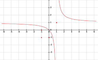
Figure 1: $T(G;x,y)$ is polynomial-time computable on the hyperbola $(x-1)(y-1)=1$ and the points $(1,1),(-1,-1),(0,-1),(-1,0)$. Otherwise it is $\mathrm{\mathbf{\sharp P}}$-hard.

4.2 Planar and bipartite planar graphs

The method of Kasteleyn [57] for tractable computation of the Ising partition function on planar graphs carries over to the Tutte polynomial.

Theorem 5 (P. Kastelyn, [57])

For planar graphs evaluating the Tutte polynomial on the hyperbola

$$H_{2}\equiv((x-1)(y-1)=2)\,,$$

is in ${\mathbf{P}}$. Otherwise, points which are $\mathrm{\mathbf{\sharp P}}$-hard on general graphs remain $\mathrm{\mathbf{\sharp P}}$-hard even on bipartite planar graphs.

Jaeger and Welsh studied the complexity of evaluating the Tutte polynomial on the class of graphs which are both bipartite and planar.

Theorem 6 (D. Vertigan and D. Welsh [88], [87])

Let $H_{\mathit{b-p}}$ be the union of $H_{1}$, $H_{2}$, and $\{(1,1),(-1,-1),(j,j),(j,j)\}$. For every $(a,b)\in\mathbb{C}^{2}$:

1. If $(a,b)\not\in H_{b-p}$, then $T(G;a,b)$ is $\mathrm{\mathbf{\sharp P}}$-hard for bipartite planar graphs.

2. If $(a,b)\in H_{b-p}$, then $T(G;a,b)$ is computable in polynomial-time for bipartite planar graphs.

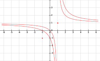
Figure 2: $T(G;x,y)$ is polynomial-time computable on the hyperbolas $(x-1)(y-1)=\{1,2\}$ and the points $(1,1),(-1,-1)$ for bipartite planar graphs. Otherwise it is $\mathrm{\mathbf{\sharp P}}$-hard.

See Figure 2 for a plot of the Tutte plane for bipartite planar graphs.

4.3 Graphs of bounded tree-width and clique-width

The Tutte polynomial and variants of it are efficiently computable on graphs of bounded tree-width or clique-width.

J. Oxley and D. Welsh initiated the study of the complexity of evaluating the Tutte polynomial on graph classes of bounded width, [74]. However, their notion of width is more restricted than tree-width, but does include the series-parallel graphs, which are of tree-width $2$. The first general results on the computation of the Tutte polynomial on graphs of bounded tree-width were obtained independently by A. Andrzejak [1] and S. Noble [71]. They proved that for every fixed evaluation $(a,b)$ of $T(G;x,y)$, there an algorithm which computes $T(G;a,b)$ using a linear number of arithmetic operations.

Theorem 7 (A. Andrzejak [1], S. Noble [71])

$T(G;x,y)$ can be evaluated in linear time in $|V|$ on graphs with bounded tree-width. In fact, $T(G;x,y)$ is fixed-parameter tractable with respect to tree-width.

Analogues of Theorem 7 for variants of the Tutte polynomial are given below. The coefficients of the Tutte polynomial and its variants can be computed in polynomial-time on graphs of bounded tree-width. In the case of $T(G;x,y)$, the list of coefficients can be computed in time $O(|V|^{3})$ by evaluating $T(G;x,y)$ at sufficiently many points to interpolate it. There is a matching cubic lower bound for the computation of all the coefficients [71].

The result [1] and [71] has a wide generalization based on logical techniques which covers colored versions of the Tutte polynomial, the Jones polynomial in knot theory, and many other graph polynomials which can be defined in Monadic Second Order logic.

T. Zaslavsky [90, 91] defined a generalization of the Tutte polynomial with an edge coloring function $c:E\to\lambda$ called the the signed Tutte polynomial for graphs and normal function of the colored matroid , respectively. This was rediscovered by Bollobás and Riordan [18] as colored versions of the Tutte polynomial.

Theorem 8 (I. Averbouch, B. Godlin and J. Makowsky [4], [63])

1. Evaluating the Tutte polynomial for signed graphs and normal function of a colored graph is fixed-parameter tractable with respect to tree-width, [4].

2. Let $\Lambda$ be a finite set. Evaluating the colored Tutte polynomial

   $$T_{\mathit{colored}}(G,c;x_{\lambda},y_{\lambda},X_{\lambda},Y_{\lambda}:\,\lambda\in\Lambda)$$

   for colored graphs $(G,c)$ with $c:E\to\Lambda$ is fixed-parameter tractable with respect to tree-width, [63].

Similar theorems stated for knot diagrams rather than graphs can be found in [64]. A detailed discussion of the signed and colored Tutte polynomials can be found in Chapter 17.1. The Jones polynomial and other relatives of the Tutte polynomial and their application to knot theory are discussed in Chapter NN (X. YYY).

The complexity of the algorithms given in [63] and [4] is asymptotically the same as in [1] and [71]. However, the runtimes of the algorithms given in [63] and [4] work also for the signed or colored Tutte polynomials, but involve very large constants due to the generality of the logical methods involved which make them impractical. The algorithms given in [1] and [71] give workable upper bounds, but do not work for the signed or colored Tutte polynomials. A more efficient algorithm for the colored Tutte polynomial was given in [82] based on [1].

Finally, Noble in [72] extended his approach to a further generalization of the Tutte polynomial, the weighted graph polynomial $U$. He showed that evaluating the weighted graph polynomial $U(G;\bar{x},y)$ is also fixed-parameter tractable with respect to tree-width.

On graphs of bounded clique-width the Tutte polynomial can be computed in subexponential time. However, unlike the case of tree-width, $T(G;x,y)$ is unlikely to be fixed-parameter tractable with respect to clique-width.

Theorem 9 (O. Giménez, P. Hliněný and M. Noy [40])

$T(G;x,y)$ can be computed in time $\exp\left(O(|V|^{1-1/(k+2)})\right)$ on graphs of clique-width at most $k$.

Theorem 10

(F. Fomin, P. Golovach, D. Lokoshtanov and S. Saurabh [35, 36])  
Given a graph $G$ and $r\in{\mathbb{N}}$, deciding whether $\chi(G;r)\neq 0$ is not fixed-parameter tractable with respect to clique-width (under the complexity-theoretic assumption $\mathrm{\mathbf{FPT}}\not=\mathrm{\mathbf{\sharp W[1]}}$). In particular, this shows that the same applies to evaluating the chromatic polynomial.

The chromatic polynomial, however, is polynomial-time computable if the clique-width is fixed:

Theorem 11

(J. Makowsky, U. Rotics, I. Averbouch and B. Godlin [66])  
The chromatic polynomial $\chi(G,\lambda)$ can be computed in time $O(|V|^{f(k)})$ on graphs of clique-width at most $k$, where $f(k)=O(2^{k})$ is a function depending only on $k$.

It is open whether Theorem 9 can be improved to match the bound for the chromatic polynomial given in Theorem 11.

We summarize the results of Sections 4.1-4.3 in Table 1.

Graph class	$\sharp{\mathbf{P}}$-hard	subexponential	${\mathbf{FPT}}$	${\mathbf{P}}$	Theorem
All graphs	${\mathbb{C}}^{2}-H$	$H$	$H$	$H$	4
planar	${\mathbb{C}}^{2}-H_{2}$	$H_{2}$	$H_{2}$	$H_{2}$	5
bipartite planar	${\mathbb{C}}^{2}-H_{b-p}$	$H_{b-p}$	$H_{b-p}$	$H_{b-p}$	6
$TW(k)$	$\emptyset$	${\mathbb{C}}^{2}$	${\mathbb{C}}^{2}$	$H$	7
$CW(k)$	$\emptyset$	${\mathbb{C}}^{2}$	$H$	$H$	9

Table 1: The complexity of evaluating the Tutte polynomial for various graph classes

.

4.4 Exact computation of the $T(G;x,y)$ on small graphs

Computing the Tutte polynomial on large graphs is a major challenge. The deleting-contraction reduction formula of the Tutte polynomial gives a naive algorithm for computing the list of coefficients of the Tutte polynomial whose runtime is exponential in the number of edges of the graph. Sekine, Imai and Tani [78] gave an algorithm computing the Tutte polynomial of a planar graph of order $n$ whose runtime is $O(2^{O(\sqrt{n})})$. Björklund et al. [7] gave an algorithm for general graphs which is exponential in the number of vertices and uses polynomial space. Haggard, Pearce and Royle [45] implemented an algorithm which exploits isomorphisms in the computation tree to allow more efficient computation of the Tutte polynomial and used it disprove a conjecture by Welsh on the roots of the Tutte polynomial. See Chapter XX for more details.

4.5 An exponential-time dichotomy theorem

An algorithm has subexponential running time if it runs in time $2^{n^{o(1)}}$. While there are subexponential algorithms for the Tutte polynomial on restricted classes of graphs [40, 78], a subexponential algorithm for the class of all graphs is unlikely to exist. Dell et al. [28] gave a dichotomy theorem which matches the vertex-exponential algorithm of [7] under the assumption that there is no subexponential algorithm for the number of proper $3$-colorings. This assumption is called the counting Exponential Time Hypothesis ($\mathrm{\mathbf{\sharp ETH}}$).

Theorem 12

(H. Dell, T. Husfeldt, D. Marx, N. Taslaman, M. Wahlen [28])
Let $(a,b)\in\mathbb{Q}^{2}$. Under $\mathrm{\mathbf{\sharp ETH}}$:

1. $T(G;a,b)$ cannot be computed in subexponential time in $|V|$ if $(a,b)\notin H_{1}$ and $b\notin\{-1,0,1\}$.

2. $T(G;a,b)$ cannot be computed in subexponential time in $|V|$ if $y=0$ and $a\notin\{-1,0,1\}$ on simple graphs.

3. $T(G;a,b)$ cannot be computed in subexponential time in $(|E|/\log^{2}|E|))$ if $a=1$ and $b\not=1$ on simple graphs.

4. $T(G;a,b)$ cannot be computed in subexponential time in $(|E|/\log^{3}|E|))$ if $(a-1)(b-1)\not=\{0,1\}$ and $(a,b)\notin\{(-1,-1),(-1,0),(0,-1)\}$ on simple graphs.

The line $y=1$ is still open ($\mathrm{\mathbf{\sharp P}}$-hardness is the best known).

Using results of R. Curticapean [26] (iii) and (iv) can be improved by eliminating the logarithmic factor.

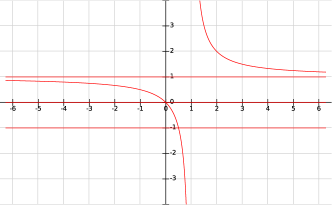
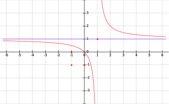
(a)                                        (b)

Figure 3: (a) Except for the hyperbola $(x-1)(y-1)=1$ and the lines $y\in\{0,-1,1\}$, $T(G;x,y)$ cannot be computed in subexponential vertex-time. (b) Except for the hyperbola $(x-1)(y-1)=1$, the line $y=1$ and the points $(-1,-1),(-1,0),(0,-1)$, $T(G;x,y)$ cannot be computed in time which is subexponential in $|E|/\log^{3}|E|$ on simple graphs.

See Figure 3 for plots of subexponential lower bounds for $T(G;x,y)$.

5 Background II

Matroids were introduced in Chapter 8 (J. Oxley) and further discussed in Chapter 11 (E. Gioan). For convenience of the reader we repeat some of the basic definitions here. A matroid is an ordered pair $(E,\mathcal{C})$ consisting of a finite set $E$, called the ground set and a set $\mathcal{C}$ of subsets of $E$, called the circuits which satisfy the following conditions:

(C1)

$\emptyset\not\in\mathcal{C}$

(C2)

If $C_{1},C_{2}\in\mathcal{C}$ and $C_{1}\subseteq C_{2}$ then $C_{1}=C_{2}$.

(C3)

If $C_{1},C_{2}\in\mathcal{C},C_{1}\neq C_{2}$ and $e\in C_{1}\cap C_{2}$ then there is $C_{3}\in\mathcal{C}$ such that $C_{3}\subseteq(C_{1}\cap C_{2})-\{e\}$.

Matroids have many equivalent definitions, cf. [89, 46] or Chapter 8, Section 4 (J. Oxley). Instead of $\mathcal{C}$ one can consider $\mathcal{I}$, the independent sets, $\mathcal{S}$, the spanning sets, $\mathcal{F}$, the flats, $\mathcal{B}$, the bases, $\mathcal{H}$, the hyperplanes. Other definitions use a closure operator on the subsets of $E$, a rank function or a girth function. All these definitions of matroids are equivalent from an axiomatic point of view, but differ from an algorithmic point of view, cf. [46, 67].

For convenience we repeat here also the definition of a matroid via a rank function from Chapter 8. Chapter 8 (J. Oxley) Let $E$ a finite set. A function $r:2^{E}\rightarrow{\mathbb{Z}}$ is a rank function if it satisfies the following conditions:

(R1)

If $X\subseteq E$ then $0\leq r(X)\leq|X|$.

(R2)

If $X\subseteq Y\subseteq E$, then $r(X)\leq r(Y)$.

(R3)

If $X,Y\subseteq E$, then

$$r(X)+r(Y)\leq r(X\cup Y)+r(X\cap Y)$$

For $A\subseteq E$, $|A|-r(A)$ is called the corank or nullity of $A$. A nonempty set $A\subseteq E$ is a circuit if $r(A)=|A|+1$ and for every $e\in E$ we have that $r(A-\{e\})=r(A)$.

Here is another equivalent definition of matroids using a girth function, cf. [46]. It is introduced here, because we will discuss its computational power as a matroid oracle in Theorem 15. Let $E$ a finite set. A function $g:2^{E}\rightarrow{\mathbb{N}}\cup\{\infty\}$ is a girth function if it satisfies the following conditions for all $X,Y\subseteq E$ and $x\in E$:

(G1)

If $g(X)<\infty$ there is $Y\subseteq X$ with $g(X)=g(Y)=|Y|$.

(G2)

If $X\subseteq Y\subseteq E$, then $g(X)\geq g(Y)$.

(G3)

If $g(X)=|X|$, $g(Y)=|Y|$, $X\neq Y$ and $x\in X\cap Y$, then
$g(X\cup Y-\{x\})<\infty$.

In all the definitions of matroids there is an exponential gap between the size of the underlying set $E$, and the information needed to capture the properties of the family of subsets, the closure operation, the rank function or the girth function defining the matroid. In order to develop a complexity theory for matroid problems three approaches are used: matroid oracle computations the restriction to matroids with succinct presentations, and using the full listing of the family of subsets (circuits, independent sets, etc.) or the functions on the subsets of the ground sets (rank function, closure operation, etc.). Pioneering papers for the first two approaches are [31, 32, 17, 77, 46, 54]. More recent discussions can be found in [67, 80].

5.1 Succinct presentation of matroids

Let $\mathcal{A}$ be a class of matroids closed under matroid isomorphisms, and $\Sigma^{*}$ be the finite words over a finite alphabet $\Sigma$. Let $\ell(w)$ denote the length of $w\in\Sigma^{*}$. and $\mathcal{A}_{n}$ the class of matroids in $\mathcal{A}$ with ground set $\{1,\ldots,n\}=[n]$ of size $n$. A class of matroids has a succinct description, or is succinct, if there is an injective mapping $e:\mathcal{A}\rightarrow\Sigma^{*}$ and a polynomial $p\in\mathbb{N}[X]$ such that for each $M\in\mathcal{A}_{n}$ we have that $\ell(e(M))\leq p(n)$. It is easy to see that $\mathcal{A}$ is succinct iff $|\mathcal{A}_{n}|=O(2^{q(n)})$ for some $q\in\mathbb{N}[X]$.

Examples 13

1. The graphic matroids are succinct using the underlying graph as their description.

2. The binary matroids, are succinct. The same is true for the matroids which can be represented over any finite field.

3. The regular matroids are the matroids which are representable over every field. Hence they form a succinct class of matroids, cf. Chapter 8, Theorem 8.16. If $M$ is regular, so is its dual. Graphical matroids are regular.

4. Transversal matroids, defined in Oxley’s Chapter 8, are representable over sufficiently large (finite) fields, hence they form a succinct class of matroids (cf. [19, Theorem 2.5]. Special cases of transversal matroids are

   1. The class of bicircular matroids . Given a graph $G$, its bicircular matroid $B(G)$ is given by $E=E(G)$ and its independent sets are the edge sets in which each connected component contains at most one cycle.

   2. The class of lattice-path matroids . A lattice path matroid is a transversal matroid that has a presentation by a collection of intervals in the ground set, relative to some fixed linear order, such that no interval contains another, cf. [19, Section 4.2].

In this chapter complexity results are always formulated for succinct classes of matroids.

The uniform matroid $U_{r,n}$ has an underlying set $E$ with $n$ elements and its basis consists of all the subsets of $E$ with exactly $r$ elements. The uniform matroids are succinct. We assume the reader is familiar with the following operations on matroids, cf. Chapter 8 (J. Oxley) Let $M,N$ be two matroids and $e,f$ be an edge of $M$ and $N$ respectively.

1. $M_{-e}$ is the matroid obtained from $M$ by deleting $e$.

2. $M_{\backslash e}$ is the matroid obtained from $M$ by contracting $e$.

3. $M\sqcup_{e,f}N$ is the $2$-sum of $M$ and $N$.

4. $M\otimes N$ is the tensor product of $M$ and $N$. Here $N$ is a pointed matroid with distinguished edge $d$. In the case $N$ is a uniform matroid $U_{r,n}$ the result is independent of the choice of $d$ in $U_{r,n}$.

Let $M$ be an arbitrary matroid. The $k$-stretch $s_{k}(M)$ is defined as $s_{k}(M)=M\otimes U_{k,k+1}$, and the $k$-thickening $t_{k}(M)$ is defined as $s_{k}(M)=M\otimes U_{1,k+1}$.

Definition 14 ([53, 86])

1. A class of matroids $\mathcal{C}$ is closed under expansions if it is closed under $s_{k}(M)$ and $t_{s}(M)$ for every $k\in{\mathbb{N}}$.

2. $\mathcal{C}$ is expand-succinct or a $\mathrm{JVW}$-class if it is succinct and $s_{k}(M)$ and $t_{k}(M)$ can be constructed in polynomial time for each $M\in\mathcal{C}$.

Typical $\mathrm{JVW}$ classes are the graphic matroids, the regular matroids, and matroids representable over a fixed finite field. The class of transversal matroids is not a $\mathrm{JVW}$-class. It is closed under deletion, but not under contraction, cf. Section 8.7 in Chapter 8.

5.2 Matroid oracles

Matroid oracles are used to show that most matroid properties are hard to compute for general matroids, cf. [77, 54]. This is largely due to the fact that the number of matroids with underlying set $E$ of size $n$ is doubly exponential in $n$. Oracles may vary, cf. [46], but the most widely used is the independence oracle, which takes as its input a set of matroid elements, and returns as output a Boolean value, true if the given set is independent and false otherwise. Naturally, every one of the nine axiomatic definitions of matroids, $\mathrm{INDEPENDENT}$, $\mathrm{BASIS}$, $\mathrm{CIRCUIT}$, $\mathrm{SPANNING}$, $\mathrm{FLAT}$, $\mathrm{HYPERPLANE}$, $\mathrm{RANK}$, $\mathrm{GIRTH}$ and $\mathrm{CLOSURE}$, gives rise to an oracle. The oracles return Boolean values also for basis sets, circuits, spanning sets, flats and hyperplanes. In the case of the rank or girth function, the oracle returns an element of $\{0,1,\ldots,|E|,\infty\}$, and in the case of the closure a subset of $E$. The computational strength of the different oracles can be compared by polynomial time simulation: Let $O_{1},O_{2}$ be two oracles of matroids on a ground set $E$. We say that $O_{1}$ is polynomially reducible to $O_{2}$, denoted by $O_{1}\rightarrow O_{2}$, iff one call in $O_{1}$ can be simulated by at most polynomially many calls on $O_{2}$.

Theorem 15 (D. Hausmann and B. Korte, [46])

Under the partial order of polynomial reducibility we have:

1. $\mathrm{BASIS}$, $\mathrm{CIRCUIT}$, $\mathrm{FLAT}$, $\mathrm{HYPERPLANE}$ are incomparable and weaker as oracles than $\mathrm{RANK}$.

2. $\mathrm{RANK}$, $\mathrm{INDEPENDENT}$, $\mathrm{SPANNING}$ and $\mathrm{CLOSURE}$ polynomially bi-reducible.

3. $\mathrm{GIRTH}$ is strictly stronger than all the other oracles.

Many natural matroid parameters are hard to compute, [54]:

Theorem 16

The following are not polynomial-time computable using the $\mathrm{INDEPENDENT}$-oracle:

1. Decide whether $M$ is uniform, self-dual, orientable, bipartite, Eulerian or representable.

2. Compute the girth or the connectivity of $M$.

3. Count the number of circuits, bases, hyperplanes or flats of $M$.

However, to the best of our knowledge, there are no papers studying the degrees of computability for oracle computations on matroids.

5.3 Full presentations of matroids

A matroid is essentially a finite set with a structured family of subsets, which can be described explicitly. This approach has originally not been studied, because the input for a Turing machine was considered too large, if the size of the matroid should be polynomial in the size of the cardinality of the ground set $E$. It was suspected, that this would make most, if not all computational matroid problems solvable in polynomial time in the size of its true input. However, D. Mayhew analyzed the situation carefully, [67], by comparing the various input sizes of $\mathrm{RANK}$, $\mathrm{INDEPENDENT}$, $\mathrm{SPANNING}$, $\mathrm{BASIS}$, $\mathrm{CIRCUIT}$, $\mathrm{FLAT}$ and $\mathrm{HYPERPLANE}$.

Suppose that $\mathrm{INPUT}_{1}$ and $\mathrm{INPUT}_{2}$ are two methods for describing a matroid $M$. Then $\mathrm{INPUT}_{1}\leq\mathrm{INPUT}_{2}$ iff there exists a polynomial-time Turing machine which will produce for every matroid $M$ the presentation $(M,\mathrm{INPUT}_{2})$ given the presentation $(M,\mathrm{INPUT}_{1})$. We write $\mathrm{INPUT}_{1}<\mathrm{INPUT}_{2}$ iff it is not the case that $\mathrm{INPUT}_{2}\leq\mathrm{INPUT}_{1}$. Surprisingly, comparing input modes gives a different picture than comparing matroid oracles.

Theorem 17 (D. Mayhem, [67])

Under the partial ordering of $\leq$ we have

1. $\mathrm{RANK}<\mathrm{INDEPENDENT}$, and $\mathrm{RANK}<\mathrm{SPANNING}$. Furthermore $\mathrm{INDEPENDENT}$ and $\mathrm{SPANNING}$ are incomparable.

2. $\mathrm{SPANNING}<\mathrm{BASIS}<\mathrm{CIRCUIT}$ and $\mathrm{BASIS}<\mathrm{HYPERPLANES}$. Furthermore, $\mathrm{CIRCUITS}$ and $\mathrm{HYPERPLANES}$ are incomparable.

3. $\mathrm{INDEPENDENT}<\mathrm{FLATS}<\mathrm{HYPERPLANES}$ and $\mathrm{INDEPENDENT}<\mathrm{BASIS}$. Furthermore, $\mathrm{BASIS}$ and $\mathrm{FLATS}$ are incomparable.

5.4 Comparing notions of matroid computability

For succinct presentations of matroids decision and counting problems can be found in most time-complexity classes between polynomial time and exponential time, because this includes graph matroids.

Complexity results for matroid oracle are usually of the form

There exists no polynomial $\mathrm{ORACLE}$-algorithm for computing $\mathrm{PROBLEM}$.

In [46] twenty problems are listed for which this is true for $\mathrm{INDEPENDENT}$, among them also the problem of computing the Tutte polynomial for arbitrary matroids.

It remains open how to work out the details needed to refine complexity results for matroid oracles analogue to the case of succinct presentations. For which problems is there an analogue to ${\mathbf{NP}}$-completeness or $\mathrm{\mathbf{\sharp P}}$-completeness in the oracle setting.

Finally, in the case of full descriptions of the matroids, it is not the case that, as one might naively suspect, that all natural problems are in ${\mathbf{P}}$. The situation is well illustrated by the following problem:

Problem: 3-matroid-intersection $\mathrm{3MI}$
Instance: An integer $k$ and three matroids $(M_{i},\mathrm{INPUT})$, $1\leq i\leq 3$ over the same ground set $E$.
Question: Does there exist a set $A\subseteq E$ such that $|A|=k$ and $A$ is independent in each $M_{i}$?

Theorem 18 (D. Mayhem, [67])

1. If $\mathrm{CIRCUITS}\leq\mathrm{INPUT}$ or $\mathrm{HYPERPLANES}\leq\mathrm{INPUT}$, then $\mathrm{3MI}$ is ${\mathbf{NP}}$-complete.

2. If $\mathrm{INPUT}\leq\mathrm{BASIS}$, then $\mathrm{3MI}$ is in ${\mathbf{P}}$.

To the best of our knowledge, the complexity of the Tutte polynomial has not been established in the full description framework.

5.5 Matroid width

J. Oxley and D. Welsh in [74] introduce a very restriced notion of matroid width: A class of matroids $\mathcal{M}$ has OW-width $k$ if a largest $3$-connected member of $\mathcal{M}$ has a groundset of $k$ elements. They show that, under some stronger assumption than succinct representability, evaluating the Tutte polynomial on matroid classes of bounded OW-width a in $\mathrm{\mathbf{FPT}}$. We shall not persue this further.

A branch decomposition of a matroid $M$ with ground set $E$ and rank function $r$ is a tree $T$ such that

1. all inner nodes of $T$ have degree three, and

2. the leaves of $T$ are in one-one correspondence with $E$.

An edge $e$ of $T$ splits $T$ into two subtrees with leaves corresponding to $E_{1}(e)$ and $E_{2}(e)$ which partition $E$. The width of $e$ is defined by $r(E_{1}(e))+r(E_{2}(e))-r(E)+1$. The width of the branch decomposition $T$ is the maximum width of an edge of $T$. Finally the branch-width of $M$ is the minimum width of the branch decompositions of $M$, and is denoted by $\mathrm{bw}(M)$.

We collect some basic facts listed in the survey paper [49].

Theorem 19

1. The branch-width of a bridgeless graph (every edge is contained in a cycle) equals the branch-width of its cycle matroid.

2. Given a matroid $M$ with $n$ elements, and a positive integer $k$, it is possible to test, using an $\mathrm{INDEPENDENT}$-oracle, in polynomial-time (with the degree depending on $k$), whether $\mathrm{bw}(M)\leq k$.

3. For matroids $M$ representable over a fixed finite field, deciding whether $\mathrm{bw}(M)\leq k$ is in ${\mathbf{FPT}}$ (fixed parameter tractable). If so, then the same algorithm also outputs a branch-decomposition of $M$ of width at most $3k$.

Although testing whether $\mathrm{bw}(M)\leq k$ is easy to check in the oracle framework, applications usually require that the matroid be representable, which is hard by Theorem 16. To remedy this, other notions of matroid width were recently introduced: decomposition width in [60] and amalgam width in [62]. Without going into details we note that matroids of decomposition width $\mathrm{dw}(M)=k$ (amalgam width $\mathrm{aw}(M)=k$) can be represeted by a decomposition tree (amalgam tree), although this tree is not known to be computable in polynomial time. However, if the decomposition or amalgam tree is given together with $M$ and is of width $k$, then many parameters can be computed in polynomial time using the $\mathrm{INDEPENDENT}$-oracle, [60, 62]. We also note that for matroids $M$ representable by a finite field $\mathbb{F}$ and branch-width $\mathrm{bw}(M)\leq k$ both $\mathrm{dw}(M)$ and $\mathrm{aw}(M)$ are bounded by functions which depend on $k$ and the size of $\mathbb{F}$.

6 The exact complexity of the Tutte polynomial for matroids

The paper [53] was the first to analyze the complexity of evaluating the Tutte polynomial for pairs of algebraic numbers $x_{0},y_{0}\in\mathbf{A}$ also for matroids. The Tutte polynomial of a graphic matroid $M(G)$ is the same as the Tutte polynomial of $G$. So here we only discuss classes of non-graphic matroids.

6.1 Succinct presentations

For the case of a class $\mathcal{C}$ matroids, the analogue of Theorem 4 uses two assumptions on the class $\mathcal{C}$ which are trivially satisfied for the class $\mathcal{G}$ of all graphic matroids. We have introduced these assumptions in Section 5 to define a $\mathrm{JVW}$-class of matroids. A $\mathrm{JVW}$-class has to be succinct, closed under $k$-stretching and $k$-thickening for all $k\in{\mathbb{N}}$, the operations of stretching and thickening have to be computable in polynomial time.

Theorem 20 (F. Jaeger, D. Vertigan and D. Welsh [53])

Let $\mathcal{C}$ be $\mathrm{JVW}$-class of matroids and $M\in\mathcal{C}$. Then evaluating $T(M;a,b)$ is $\mathrm{\mathbf{\sharp P}}$-hard on all points $(a,b)\not\in H$. If $(a,b)\in H$, then $T(M;a,b)$ is computable in polynomial time.

Here $H$ is the same as in Theorem 4.

The class of transversal matroids $\mathcal{T}$ is succinct, cf. Example 13. However, it is not a $\mathrm{JVW}$-class. We still have the following dichotomy:

Theorem 21 (C. Colbourn, J. Provan and D. Vertigan, [22])

For the class of transversal matroids $M\in\mathcal{T}$ the evaluation the Tutte polynomial $T(M,x_{0},y_{0})$ is $\mathrm{\mathbf{\sharp P}}$-hard for all $(x_{0},y_{0})\in\mathbf{A}$, unless $(x_{0}-1)(y_{0}-1)=0$, in which case it is in ${\mathbf{P}}$.

To prove this theorem, the authors replace the operations $k$-stretching and $k$-thickening used in the proof of Theorem 20 by operations $k$-expansion and $k$-augmentation which preserve transversality.

A bicircular matroid of a graph $G$ is the matroid $B(G)$ whose points are the edges of $G$ and whose independent sets are the edge sets of pseudoforests of $G$, that is, the edge sets in which each connected component contains at most one cycle. The class $\mathcal{B}$ of bicircular matroids is contained in the class $\mathcal{T}$ of transversal matroids, which, unlike transversal matroids, is closed under minors. A bicircular matroid $B=B(G)$ is determined by its underlying graph $G$, but it need not be graphic. The $k$-stretching of a bicircular matroid $B$, denoted by $s_{k}(B)$ can be shown to be $B(s_{k}(G))$. Hence, bicircular matroids are closed under $k$-stretching. However, they are not closed under $k$-thickening.

Theorem 22 ([41])

For a matroid $M\in\mathcal{B}$, the evaluation of the Tutte polynomial $T(M,X,Y)$ is $\mathrm{\mathbf{\sharp P}}$-hard for all $(x_{0},y_{0})\in\mathbf{A}$, unless $(x_{0}-1)(y_{0}-1)=0$. For $x_{0}=0$ and $x_{0}=-1$ the complexity has not yet been determined.

Proposition 23 ([41])

For the complete graph $K_{n}$ and the bicircular matroid $M=B(K_{n})\in\mathcal{B}$, the evaluation of the Tutte polynomial $T(M,x_{0},y_{0})$ is in $\mathrm{\mathbf{P}}$.

A further special case of transversal matroids is the class of the lattice-path matroids $\mathcal{LP}$. They are obtained from the lattice with vertices in $(i,j)\in{\mathbb{N}}^{2}$ with $0\leq i\leq m$ and $0\leq j\leq r$ with steps $\mathrm{EAST}$ and $\mathrm{NORTH}$. Let $P$ and $Q$ be two paths in this lattice. The lattice paths that go from $(0,0)$ to $(m,r)$ and that remain in the region bounded by $P$ and $Q$ can be identified with the bases of a particular type of transversal matroid, [20].

Theorem 24 ([69])

For lattice-path matroids $M\in\mathcal{LP}$, the evaluation of the Tutte polynomial $T(M,x_{0},y_{0})$ is in $\mathrm{\mathbf{P}}$.

6.2 Matroid oracles

The situation for matroids which have no succinct presentation the situation is less understood.

We summarize here what is known about the computability of the Tutte polynomial when the matroid is given by an oracle.

Theorem 25

Let $M$ be a matroid of size $n$ and rank $r$. Using the $\mathrm{INDEPENDENT}$-oracle we have

1. The Tutte polynomial $M$ is not computable in polynomial time, [54].

2. If the the matroid $M$ has branch-width $\mathrm{bw}(M)\leq k$ and is representable over a finite field $\mathbb{F}$, then $T(M,x,y)$ is computable in time $O(n^{6}\log(n)\log\log(n))$ even without the oracle, [48].

3. If $M$ has decomposition-width $\mathrm{dw}(M)\leq k$ and is given with its decomposition tree, then $T(M,x,y)$ is computable in time $O(k^{2}n^{3}r^{2})$ and evaluated in time $O(k^{2}n)$ (under the assumption of unit cost of the arithmetic operations), [60].

4. If $M$ has amalgam-width $\mathrm{aw}(M)\leq k$ and is given with its amalgam tree, then $T(M,x,y)$ is computable in time $O(n^{d})$ for some constant $d$ independent of $k$, [62].

7 Tutte polynomial in algebraic models of computation

The complexity of the Tutte polynomial was also studied in various alternative models of computation.

7.1 Valiant’s algebraic circuit model

L. Valiant introduced in [85] an algebraic model of computation based on uniformly defined families of algebraic circuits and a notion of reducibility based on substitutions called p-projections. In this framework it is natural to consider multivariate versions of graph polynomials, see also see also Chapter 18 (Traldi). In this model there is analogue for polynomial time called $\mathrm{\mathbf{VP}}$ and for non-deterministic polynomial time called ${\mathbf{VNP}}$. Computing the family of determinants $\mathrm{DET}_{n}$ of an $(n\times n)$ matrix where the entries are treated as indeterminates is in $\mathrm{\mathbf{VP}}$, computing the corresponding permanent $\mathrm{PER}_{n}$ is ${\mathbf{VNP}}$-complete. The major problem in Valiant’s framework is the question whether $\mathrm{\mathbf{VP}}={\mathbf{VNP}}$. A detailed development of Valiant’s theory can be found in [21].

Typical families of functions in ${\mathbf{VNP}}$ are generating functions of graph properties. These are polynomials depending on graphs with indeterminate weights on the edges. Let $\mathcal{P}$ be a graph property, i.e., a class of finite graphs closed under isomorphisms. For a graph $G=(V(G),E(G))$ the generating function of a graph property is defined as

$$GF(G,\mathcal{P})=\sum_{E^{\prime}\subseteq E,(V(G),E^{\prime})\in\mathcal{P}}\prod_{e\in E^{\prime}}X_{e}$$

The complexity of generating functions of graph properties in Valiant’s model was first studied by M. Jerrum in [55] and further developed by P. Bürgisser in [21].

The Tutte polynomial of a graph has only two variables, therefore it cannot be ${\mathbf{VNP}}$-complete in Valiant’s model. In order to get a complete family of Tutte polynomials we have to put weights on the edges of the underlying graph. This leads to a weighted Tutte polynomial as defined in [81] or in [18]. Let $G=(V(G),E(G))$ be a graph. For each $e\in E(G)$ we have four indeterminates $X_{e},Y_{e},x_{e},y_{e}$. Fix an order on the edges $E(G)$. The multivariate Whitney rank generating function $W(G_{n};X_{e},Y_{e},x_{e},y_{e})$ is defined for connected graphs $G$ by

$$W(G_{n};X_{e},Y_{e},x_{e},y_{e})=$$

$$\sum_{T\subseteq E(G)}\prod_{e\in T,int-act}X_{e}\prod_{e\in E(G)-T,ext-act}Y_{e}\prod_{e\in T,int-inact}x_{e}\prod_{e\in E(G)-T,ext-inact}y_{e}$$

where the sum is over all spanning trees $T$, and the condition of internal/external active/inactive is defined with respect to the order on $E(G)$. For graphs not connected we add additional indeterminates.

Traldi’s dichromatic polynomial $Q(G;v_{e},q,z)$ is defined by

$$Q(G;v_{e},q,z)=\sum_{E^{\prime}\subseteq E(G)}q^{k(E^{\prime})}z^{|E^{\prime}|-r(E^{\prime})}\prod_{e\in E^{\prime}}v_{e}$$

where $k(E^{\prime})$ is the number of connected components of the spanning subgraph induced by $E^{\prime}$, and $r(E^{\prime})$ is its rank.

The complexity of the Tutte polynomial in Valiant’s model was studied in [61]. To get a meaningful complexity analysis, the notion of p-projections is modified to allow also a wider class of substitutions which the authors call polynomial oracle reductions. Not surprisingly, they show that in this (slightly) modified framework of Valiant’s model the multivariate Tutte polynomial is ${\mathbf{VNP}}$-complete. More precisely:

Theorem 26 ([61])

1. There is a family of graphs $G_{n}$ such that the family of multivariate Tutte polynomials $W(G_{n};X_{e},Y_{e},x_{e},y_{e})$ is ${\mathbf{VNP}}$-complete under p-projections.

2. Traldi’s dichromatic polynomial $Q(G;v_{e},q,z)$ is ${\mathbf{VNP}}$-complete via polynomial oracle reductions.

For details the reader is referred to [61, 50].

7.2 The Blum-Shub-Smale model

In the early 1970s computability over arbitrary first order structures was introduced independently in [33, 38] by E. Engeler and H. Friedman. What they propose is, roughly speaking, to use register machines over first order structures $\mathfrak{A}$, where the registers contain elements of $\mathfrak{A}$ and the tests and operations are defined by the relations and functions of $\mathfrak{A}$. Their framework was rediscovered by L. Blum, M. Shub and S. Smale in [15], see also [14] and [39] for a comparison between [38] and [15]. They main merit of [15] is the introduction of a complexity theory for computability over the real and complex numbers which includes complexity classes ${\mathbf{P}}_{\mathcal{R}}$ for deterministic polynomial-time computable and ${\mathbf{NP}}_{\mathcal{R}}$ for non-deterministic polynomial-time computable problems, and the existence of ${\mathbf{NP}}_{\mathcal{R}}$-complete problems, where $\mathcal{R}$ is an arbitrary (possibly ordered) ring. We call this model of computation the $\mathrm{BSS}$ model of computation. Later, K. Meer, [68], introduced also a complexity class $\sharp{\mathbf{P}}_{\mathcal{R}}$ for the $\mathrm{BSS}$ model of computation.

As it is customary to look at the Tutte polynomial $T(G;x,y)$ as a polynomial in ${\mathbb{R}}[x,y]$ or ${\mathbb{C}}[x,y]$, and graphs can be viewed as $0-1$-matrices, the complexity of the Tutte polynomial is most naturally discussed in the $\mathrm{BSS}$ model of computation, [65]. However, the theory of counting complexity in the $\mathrm{BSS}$ model of computation has various drawbacks. In particular, there is no satisfactory theory for $\sharp{\mathbf{P}}_{\mathcal{R}}$-complete problems. Furthermore, it is not clear whether, and it seems unlikely that, evaluating the chromatic polynomial at the point $x=3$ is ${\mathbf{NP}}_{\mathcal{R}}$-complete. A detailed description of these problems can be found in [58, 59], where also an abstract algebraic version of the JVW-Theorem, 4, is formulated. In [2] the descriptive complexity of counting problems in the $\mathrm{BSS}$ model of computation over ${\mathbb{R}}$ is also discussed using essentially the same framework as in [58, 59].

8 Open problems

The complexity of computing or evaluating the Tutte polynomial in the Turing model of computation in a ring $\mathcal{R}[x,y]$ is well understood

• for graphs without restrictions on their presentations, and

• for matroids, provided the matroids have succinct presentations,

provided the arithmetic operations in the ring $\mathcal{R}$ are polynomial-time computable in some standard presentation of $\mathcal{R}$. The same is true for special classes of graphs (planar, bipartite, etc.) and special succinct classes of matroids (transversal, bicircular, etc.). For graph classes of bounded tree-width evaluating the Tutte polynomial is fixed parameter tractable. However, for graph classes of bounded clique-width, the situation is not completely understood.

Problem 1

Determine the complexity of evaluating the Tutte polynomial for graphs of fixed clique-width.

Planar graphs are a special cases of a minor-closed class of graphs.

Problem 2

Determine the complexity of evaluating the Tutte polynomial for other minor-closed graph classes.

The JVW Theorem, 4, and its variations show a dichotomy, the Difficult Point Property ($\mathrm{DPP}$): Evaluation of the Tutte polynomial at fixed evaluation points is $\sharp{\mathbf{P}}$ hard on all points in $\mathcal{R}^{2}-A$ where $A\subset\mathcal{R}^{2}$ is a semialgebraic (quasialgebraic) set of dimension $1$. Versions of $\mathrm{DPP}$ have been proven also for many other graph polynomials, e.g., the Bollobás-Riordan version of the Tutte polynomial, [10, 11], the interlace polynomial, [12, 13], the cover polynomial for directed graphs, [8, 9]. the bivariate matching polynomial for multi-graphs defined first in [47] in [5, 51], and many more which are surveyed in [59].

Problem 3

Characterize the graph polynomials for which $\mathrm{DPP}$ holds.

If one studies the complexity in the Turing model of computation, the real or complex numbers have no recursive presentation. Moreover, the recursive presentaions of the countable subrings which do have a recursive presentation are not uniform. This makes the statement about the complexity over the reals or complex numbers somehow artificial. In the $\mathrm{BSS}$ model of computation, cf. [59], this problem of non-uniformity does not arise.

Problem 4

Refine the complexity analysis of the Tutte polynomial in the $\mathrm{BSS}$ model of computation.

In the case of matroids without succinct presentation, it is known that the Tutte polynomial is not polynomial-time computable using the the $\mathrm{INDEPENDENT}$-oracle, Theorem 25. But to the best of our knowledge, the analogues of ${\mathbf{NP}}$-completeness, or higher levels of the complexity hierarchy within exponential time oracle computability of matroids has not been developed.

Problem 5

Develop a coherent theory of complexity for computations with matroid oracles in general.

References

- [1] A. Andrzejak. An algorithm for the Tutte polynomials of graphs of bounded treewidth. DMATH: Discrete Mathematics, 190, 1998.
- [2] M. Arenas, M. Munoz, and C. Riveros. Descriptive complexity for counting complexity classes. In Logic in Computer Science (LICS), 2017 32nd Annual ACM/IEEE Symposium on, pages 1–12. IEEE, 2017.
- [3] S. Arora and B. Barak. Computational complexity: a modern approach. Cambridge University Press, 2009.
- [4] I. Averbouch, B. Godlin, and J.A. Makowsky. An extension of the bivariate chromatic polynomial. European Journal of Combinatorics, 31(1):1–17, 2010.
- [5] I. Averbouch and J.A. Makowsky. The complexity of multivariate matching polynomials. Preprint, January 2007.
- [6] G.D. Birkhoff. A determinant formula for the number of ways of coloring a map. Annals of Mathematics, 14:42–46, 1912.
- [7] A. Björklund, T. Husfeldt, P. Kaski, and M. Koivisto. Computing the Tutte polynomial in vertex-exponential time. In Foundations of Computer Science, 2008. FOCS’08. IEEE 49th Annual IEEE Symposium on, pages 677–686. IEEE, 2008.
- [8] M. Bläser and H. Dell. Complexity of the cover polynomial. In ICALP, pages 801–812, 2007.
- [9] M. Bläser, H. Dell, and M. Fouz. Complexity and approximability of the cover polynomial. Computational Complexity, xx:xx–yy, 2012. accepted for publication.
- [10] M. Bläser, H. Dell, and J.A. Makowsky. Complexity of the Bollobás-Riordan polynomial. exceptional points and uniform reductions. In Edward A. Hirsch, Alexander A. Razborov, Alexei Semenov, and Anatol Slissenko, editors, Computer Science–Theory and Applications, Third International Computer Science Symposium in Russia, volume 5010 of Lecture Notes in Computer Science, pages 86–98. Springer, 2008.
- [11] M. Bläser, H. Dell, and J.A. Makowsky. Complexity of the Bollobás-Riordan polynomial: Exceptional points and uniform reductions. Theory Comput. Syst., 46(4):690–706, 2010.
- [12] M. Bläser and C. Hoffmann. On the complexity of the interlace polynomial. arXive 0707.4565, 2007.
- [13] M. Bläser and C. Hoffmann. On the complexity of the interlace polynomial. In STACS, pages 97–108, 2008.
- [14] L. Blum, F. Cucker, M. Shub, and S. Smale. Complexity and Real Computation. Springer-Verlag, New York, 1998.
- [15] L. Blum, M. Shub, and S. Smale. On a theory of computation and complexity over the real numbers. Bulletin of the American Mathematical Society, 21:1–46, 1989.
- [16] H.L. Bodlaender and T. Kloks. Efficient and constructive algorithms for the pathwidth and treewidth of graphs. Journal of Algorithms, 21(2):358–402, 1996.
- [17] B. Bollobás and S.E. Eldridge. Packings of graphs and applications to computational complexity. Journal of Combinatorial Theory, Series B, 25(2):105–124, 1978.
- [18] B. Bollobás and O. Riordan. A Tutte polynomial for coloured graphs. Combinatorics, Probability and Computing, 8:45–93, 1999.
- [19] J.E. Bonin. An introduction to transversal matroids, 2010.
- [20] J.E. Bonin and A. De Mier. Lattice path matroids: structural properties. European Journal of Combinatorics, 27(5):701–738, 2006.
- [21] P. Bürgisser. Completeness and reduction in algebraic complexity theory, volume 7. Springer, 2000.
- [22] C.J. Colbourn, J.S. Provan, and D.L. Vertigan. The complexity of computing the Tutte polynomial on transversal matroids. Combinatorica, 15(1):1–10, 1995.
- [23] B. Courcelle. The monadic second-order logic of graphs. i. recognizable sets of finite graphs. Information and computation, 85(1):12–75, 1990.
- [24] B. Courcelle, J.A. Makowsky, and U. Rotics. On the fixed parameter complexity of graph enumeration problems definable in monadic second-order logic. Discrete Applied Mathematics, 108(1):23–52, 2001.
- [25] B. Courcelle and S. Olariu. Upper bounds to the clique width of graphs. Discrete Applied Mathematics, 101(1):77–114, 2000.
- [26] R. Curticapean. Block interpolation: A framework for tight exponential-time counting complexity. In Automata, Languages, and Programming - 42nd International Colloquium, ICALP 2015, Kyoto, Japan, July 6-10, 2015, Proceedings, Part I, pages 380–392, 2015.
- [27] M. Cygan, F.V. Fomin, L. Kowalik, D. Lokshtanov, D. Marx, M. Pilipczuk, M. Pilipczuk, and S. Saurabh. Parameterized algorithms, volume 3. Springer, 2015.
- [28] H. Dell, T. Husfeldt, D. Marx, N. Taslaman, and M. Wahlen. Exponential time complexity of the permanent and the Tutte polynomial. ACM Trans. Algorithms, 10(4):21:1–21:32, 2014.
- [29] R.G. Downey and M.R. Fellows. Parameterized complexity. Springer Science & Business Media, 2012.
- [30] R.G. Downey and M.R. Fellows. Fundamentals of parameterized complexity, volume 4. Springer, 2013.
- [31] J. Edmonds. Minimum partition of a matroid into independent subsets. J. Res. Nat. Bur. Standards Sect. B, 69:67–72, 1965.
- [32] J. Edmonds. Matroids and the greedy algorithm. Mathematical programming, 1(1):127–136, 1971.
- [33] E. Engeler. Algorithmic properties of structures. Theory of Computing Systems, 1(2):183–195, 1967.
- [34] J. Flum and M. Grohe. Parameterized complexity theory. Springer, 2006.
- [35] F.V. Fomin, P.A. Golovach, D. Lokshtanov, and S. Saurabh. Algorithmic lower bounds for problems parameterized with clique-width. In M. Charikar, editor, Proceedings of the Twenty-First Annual ACM-SIAM Symposium on Discrete Algorithms, SODA 2010, Austin, Texas, USA, January 17-19, 2010, pages 493–502. SIAM, 2010.
- [36] F.V. Fomin, P.A. Golovach, D. Lokshtanov, and S. Saurabh. Intractability of clique-width parameterizations. SIAM Journal on Computing, 39(5):1941–1956, 2010.
- [37] F.V. Fomin and D. Kratsch. Exact exponential algorithms. Springer Science & Business Media, 2010.
- [38] H. Friedman. Algorithmic procedures, generalized turing algorithms, and elementary recursion theory. In Logic colloquium, volume 69, pages 361–389, 1970.
- [39] H. Friedman and R. Mansfield. Algorithmic procedures. Transactions of the American Mathematical Society, pages 297–312, 1992.
- [40] O. Giménez, P. Hlině,nỳ, and M. Noy. Computing the Tutte polynomial on graphs of bounded clique-width. SIAM Journal on Discrete Mathematics, 20(4):932–946, 2006.
- [41] O. Giménez and M. Noy. On the complexity of computing the Tutte polynomial of bicircular matroids. Combinatorics, Probability and Computing, 15(03):385–395, 2006.
- [42] L.A. Goldberg and M. Jerrum. The complexity of computing the sign of the Tutte polynomial. SIAM Journal on Computing, 43(6):1921–1952, 2014.
- [43] O. Goldreich. Computational Complexity: A Conceptual Perspective. Cambridge University Press, 2008.
- [44] J. Gruska. Quantum computing, volume 2005 of Advanced Topics in Computer Science Series. McGraw-Hill London, 1999.
- [45] G. Haggard, D.J. Pearce, and G. Royle. Computing Tutte polynomials. ACM Transactions on Mathematical Software (TOMS), 37(3):24, 2010.
- [46] D. Hausmann and B. Korte. Algorithmic versus axiomatic definitions of matroids. Mathematical Programming Study, 14:98–111, 1981.
- [47] C.J. Heilmann and E.H. Lieb. Theory of monomer-dymer systems. Comm. Math. Phys, 25:190–232, 1972.
- [48] P. Hliněnỳ. The Tutte polynomial for matroids of bounded branch-width. Combinatorics, Probability and Computing, 15(03):397–409, 2006.
- [49] P. Hliněný, S. Oum, D. Seese, and G. Gottlob. Width parameters beyond tree-width and their applications. Comput. J., 51(3):326–362, 2008.
- [50] C. Hoffmann. Computational Complexity of Graph Polynomials. PhD thesis, Naturwissenschaftlich-Technische Fakultät der Universität des Saarlandes, Saarbrücken, Germany, 2010.
- [51] C. Hoffmann. A most general edge elimination polynomial–thickening of edges. Fundamenta Informaticae, 98.4:373–378, 2010.
- [52] F. Jaeger. Tutte polynomials and link polynomials. Proceedings of the American Mathematical Society, 103(2):647–654, 1988.
- [53] F. Jaeger, D. L. Vertigan L, and D.J.A. Welsh. On the computational complexity of the Jones and Tutte polynomials. Mathematical Proceedings of the Cambridge Philosophical Society, 108(01):35–53, 1990.
- [54] P.M. Jensen and B. Korte. Complexity of matroid property algorithms. SIAM Journal on Computing, 11(1):184–190, 1982.
- [55] M. Jerrum. On the complexity of evaluating multivariate polynomials. Aiken Computation Lab, Departement of Computer Science, University of Edinburgh, 1981.
- [56] D.S. Johnson. A catalog of complexity classes. In J. van Leeuwen, editor, Handbook of Theoretical Computer Science, volume 1, chapter 2. Elsevier Science Publishers, 1990.
- [57] P.W. Kasteleyn. The statistics of dimers on a lattice. Physica, 27:1209–1225, 1961.
- [58] T. Kotek, J.A. Makowsky, and E.V. Ravve. A computational framework for the study of partition functions and graph polynomials. In SYNASC, pages 365–368. IEEE Computer Society, 2012.
- [59] T. Kotek, J.A. Makowsky, and E.V. Ravve. A computational framework for the study of partition functions and graph polynomials. In Proceedings of the 12th Asian Logic Conference ’11, pages 210–230, 2013.
- [60] D. Král. Decomposition width of matroids. Discrete Applied Mathematics, 160(6):913–923, 2012.
- [61] M. Lotz and J.A. Makowsky. On the algebraic complexity of some families of coloured Tutte polynomials. Advances in Applied Mathematics, 32(1):327–349, 2004.
- [62] L. Mach and T. Toufar. Amalgam width of matroids. In Parameterized and Exact Computation, pages 268–280. Springer, 2013.
- [63] J. A. Makowsky. Coloured Tutte polynomials and kauffman brackets for graphs of bounded tree width. Discrete Applied Mathematics, 145(2):276–290, 2005.
- [64] J.A. Makowsky and J.P. Mariño. The parametrized complexity of knot polynomials. Journal of Computer and System Sciences, 67(4):742–756, 2003.
- [65] J.A. Makowsky and K. Meer. On the complexity of combinatorial and metafinite generating functions of graph properties in the computational model of Blum, Shub and Smale. In CSL’00, volume 1862 of Lecture Notes in Computer Science, pages 399–410. Springer, 2000.
- [66] J.A. Makowsky, U. Rotics, I. Averbouch, and B. Godlin. Computing graph polynomials on graphs of bounded clique-width. In Graph-theoretic concepts in computer science, pages 191–204. Springer, 2006.
- [67] D. Mayhew. Matroid complexity and nonsuccinct descriptions. SIAM Journal on Discrete Mathematics, 22(2):455–466, 2008.
- [68] K. Meer. Counting problems over the reals. Theoretical Computer Science, 242(1-2):41–58, 2000.
- [69] J. Morton and J. Turner. Computing the Tutte polynomial of lattice path matroids using determinantal circuits. arXiv preprint arXiv:1312.3537, 2013.
- [70] M.A. Nielsen and I.L. Chuang. Quantum computation and quantum information. Cambridge university press, 2010.
- [71] S.D. Noble. Evaluating the Tutte polynomial for graphs of bounded tree-width. Combinatorics, Probability and Computing, 7:307–321, 1998.
- [72] S.D. Noble. Evaluating a weighted graph polynomial for graphs of bounded tree-width. Electron, J. Combin., 16(1), 2009.
- [73] S. Oum and P. Seymour. Approximating clique-width and branch-width. Journal of Combinatorial Theory, Series B, 96(4):514–528, 2006.
- [74] J.G. Oxley and D.J.A. Welsh. Tutte polynomials computable in polynomial time. Discrete Mathematics, 109(1):185–192, 1992.
- [75] C. Papadimitriou. Computational Complexity. Addison Wesley, 1994.
- [76] N. Robertson and P.D. Seymour. Graph minors. x. obstructions to tree-decomposition. Journal of Combinatorial Theory, Series B, 52(2):153–190, 1991.
- [77] G.C. Robinson and D.J.A. Welsh. The computational complexity of matroid properties. Math. Proc. Camb. Phil. Soc., 87:29–45, 1980.
- [78] K. Sekine, H. Imai, and S. Tani. Computing the Tutte polynomial of a graph of moderate size. In Algorithms and Computations, pages 224–233. Springer, 1995.
- [79] M. Sipser. Introduction to the theory of computation. PWS Publishing Company, Boston, 1997.
- [80] S. Snook. Matroids, Complexity and Computation. PhD thesis, Victoria University of Wellington, 2013.
- [81] L. Traldi. A dichromatic polynomial for weighted graphs and link polynomials. Proc. Amer. Math. Soc., 106:279–286, 1989.
- [82] L. Traldi. On the colored Tutte polynomial of a graph of bounded treewidth. Discrete Applied Mathematics, 154(6):1032–1036, 2006.
- [83] W.T. Tutte. A contribution to the theory of chromatic polynomials. Canadian Journal of Mathematics, 6:80–91, 1954.
- [84] L. G. Valiant. The complexity of enumeration and reliability problems. SIAM Journal on Computing, 8(3):410–421, 1979.
- [85] L. G. Valiant. Reducibility by algebraic projections. In Logic and algorithmic (Zurich, 1980), pages 365–380. Univ. Genève, Geneva, 1982.
- [86] D. L. Vertigan. Bicycle dimension and special points of the Tutte polynomial. Journal of Combinatorial Theory, Series B, 74(2):378–396, 1998.
- [87] D.L. Vertigan. The computational complexity of Tutte invariants for planar graphs. SIAM Journal on Computing, 35(3):690–712, 2005.
- [88] D.L. Vertigan and D.J.A. Welsh. The computational complexity of the Tutte plane: the bipartite case. Combinatorics, Probability and Computing, 1(02):181–187, 1992.
- [89] D.J.A. Welsh. Matroid Theory, volume 8 of London Mathematical Society Monographs. Academic Press, 1976.
- [90] T. Zaslavsk. Chromatic invariants of signed graphs. Discrete Mathematics, 42(2):287–312, 1982.
- [91] T. Zaslavsky. Strong Tutte functions of matroids and graphs. Transactions of the American Mathematical Society, 334(1):317–347, 1992.
Index
- clique-width §3.2, §4.3, §4.3—Definition 2
- colored Tutte polynomial §4.3
-
complexity §3.1
- counting problem §3.1
- decision problem §3.1
- fixed-parameter tractable §3.1
- FP §3.1
- FPT §3.1
- intractable §3.1
- NP §3.1
- NP-hard §3.1
- P §3.1
- parameterized §3.1
- polynomial time §3.1
- (sharp P) §3.1
- -hard §3.1
- subexponential §4.3
- subexponential time §4.5
- tractable §3.1
- VNP §7.1
- VNP-completeness §7.1
- VP §7.1
- computation model
- determinant §7.1
- dichotomy theorem
- Difficult Point Property §8
- explicit computation §4.4
- -expression §3.2
- -graph §3.2
-
matroid §5
- amalgam width §5.5
- bases §5
- bicircular item iva, §6.1
- binary item ii
- branch decomposition §5.5
- branch-width §5.5
- closure §5
- decomposition width §5.5
- flats §5
- girth function §5
- graphic item i
- hyperplanes §5
- independence oracle §5.2
- independent sets §5
- JVW-class §6.1
- lattice path §6.1
- lattice-path item ivb
- oracle computations §5
- OW-width §5.5
- rank function §5
- regular item iii
- spanning sets §5
- succinct §5.1
- transversal item iv, §6.1
- uniform §5.1
-
matroid class
- closed under expansions item i
- normal function of the colored matroid §4.3
- permanent §7.1
- the weighted graph polynomial §4.3