A search for heavy-metal stars: abundance analyses of hot subdwarfs with Subaru

Abstract

The discovery of extremely zirconium- and lead-rich surfaces amongst a small subgroup of hot subdwarfs has provoked questions pertaining to chemical peculiarity in hot star atmospheres and about their evolutionary origin. With only three known in 2014, a limited search for additional ‘heavy-metal’ subdwarfs was initiated with the Subaru telescope. Five hot subdwarfs having intermediate to high surface enrichment of helium were observed at high-resolution and analyzed for surface properties and abundances. This paper reports the analyses of four of these stars. PG 1559+048 and FBS 1749+373, having only intermediate helium enrichment, show strong lines of triply ionized lead. PG 1559+048 also shows a strong overabundance of germanium and yttrium. With more helium-rich surfaces, Ton 414 and J17554+5012, do not show evidence of heavy-metal enrichment. This limited survey suggests that extreme enrichment of ‘heavy metals’ by selective radiative levitation in hot subdwarf atmospheres is suppressed if the star is too helium-rich.

1 Introduction

The origin of hot subluminous stars which have surfaces rich in heavy metals including zirconium and lead poses a challenge. They have surfaces dominated neither by hydrogen nor by helium and belong to a group known as intermediate helium subdwarfs (iHe-sds) (Naslim et al., 2010). By convention, this group is characterized by a surface helium abundance (fractional abundance by number) $0.1<n_{\rm He}<0.9$ and corresponds approximately to a Drilling et al. (2013) helium class in the range He15 – He35 (ibid. Fig. 12). Surface temperatures and gravities cover the ranges $30\,000<T_{\rm eff}/{\rm K}<42\,000$ and $5.0<\log g/(\rm cm\,s^{-2})<6.0$.

In contrast, normal subdwarf B (sdB) stars have helium-poor atmospheres ($n_{\rm He}<0.1$) whilst helium-rich hot subdwarfs (He-sds) show surface helium abundance in a range $0.9<n_{\rm He}<0.99$ with a wide range of surface temperature $T_{\rm eff}=25\,000-45\,000$ K (Naslim et al., 2010).

During a photometric survey of 21 iHe-sds (Ahmad et al., 2004), Ahmad & Jeffery (2005) discovered evidence for g-mode pulsations in LS IV$-14^{\circ}116$, later confirmed by Green et al. (2011) and Jeffery (2011). Follow-up spectroscopy of LS IV$-14^{\circ}116$ led to the discovery of 3–4 dex overabundances of the trans-iron elements zirconium, yttrium, strontium and germanium (Naslim et al., 2011), which had not previously been found in other iHe-sds. A targeted survey of iHe-sds subsequently led to the discovery of two stars, HE 2359–2844 and HE 1256–2738, with $\approx 4$ dex overabundances of lead, together with other heavy elements (Naslim et al., 2013). More recent discoveries include Feige 46 – a pulsating ‘twin’ to LS IV$-14^{\circ}116$ (Latour et al., 2019a), and EC 22536–4304, a new lead-rich subdwarf (Jeffery & Miszalski, 2019). The over-abundance of trans-iron elements has led to these unusual stars becoming known as ’heavy-metal subdwarfs’.

The questions raised by these discoveries include the numerical frequency of heavy-metal subdwarfs amongst the population of hot subdwarfs as a whole, the range of effective temperature and surface gravity over which they occur, whether there are systematics within the group regarding which elements are enhanced, whether they occur in binaries, the evolution channel which produces subdwarfs with ’intermediate’ helium-rich surfaces, and the mechanism by which the surfaces become metal-rich. One hypothesis is that iHe-sds are in transition phase from helium-rich to helium-poor due to atmospheric diffusion processes. Atmospheric helium gradually sinks within a time-scale of 10⁵ years as the helium-rich star contracts towards the zero-age horizontal branch. In their radiation-dominated atmosphere, certain selected species concentrate into specific regions where opacities are high enough to observe extreme over-abundances. A clear theoretical account of this process is still lacking.

This paper starts to address the first two questions by reporting the results of a limited spectroscopic survey of helium-rich subdwarfs made using the High Dispersion Spectrograph (HDS) of the Subaru Telescope. One star observed in the survey, UVO 0825+15  has already been reported as a lead-rich subdwarf (Jeffery et al., 2017b). In § 2, we report the remaining observations. In § 3 and 4 we report the measurements of atmospheric parameters and abundance analyses, and in § 5 we draw interim conclusions.

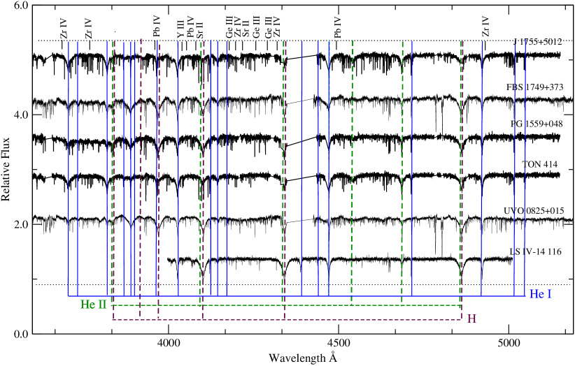
Figure 1: Subaru/HDS spectra of five helium-rich subdwarfs together with (bottom) the AAT/UCLES spectrum of LS IV$-14^{\circ}116$ from Naslim et al. (2011). Locations of pricipal H, Hei, Heii, Geiii, Yiii, Zriv and Pbiv lines are indicated.

2 Observations

Observations of five He-sds were obtained on 2015 June 3 with the HDS on the Subaru telescope in service mode (program S15A-206S). The sample analysed in this paper comprised PG 1559+048, Ton 414, FBS 1749+373, and GALEX J175548.50+501210.77. These stars were identified as He-sds sufficiently bright for high-resolution high signal-to-noise spectroscopy, and with $T_{\rm eff}$ in a range similar to that in which heavy-metals had been discovered previously (Naslim et al., 2011, 2013).

Two exposures were made consecutively for each star, with exposure times of 1200 s in each case, except for the brighter GALEX J175548.50+501210.77, where an exposure times of 300 s was used. A slit width of 0.4 mm was used, corresponding to a projected resolution $R=45\,000$. The data were reduced as described by Jeffery et al. (2017b, § 2.3). The Subaru HDS spectra of the current sample are shown in Figure 1, together with the fifth sample member UVO 0825+15 (Jeffery et al., 2017b) and the AAT spectrum of LS IV$-14^{\circ}116$ (Naslim et al., 2011).

Radial velocities ($v_{\rm r}$) measured for all four stars were reported by Martin et al. (2017). However those measurements omitted a correction to the heliocentric rest frame, and should have been given as in Table 1.

PG 1559+048 (= GALEX J160131.30+044027.00) is classified sdOA by Green et al. (1986), sdBC0.2VII:He22 by Drilling et al. (2013), and He-sdB by Németh et al. (2012), thus indicating an intermediate helium abundance. Our Subaru/HDS spectrum shows relatively strong N ii, N iii, C ii, and C iii lines, weak Si iii, Si iv, S iii, and Ca iii lines, together with strong hydrogen Balmer, He i and He ii 4686 Å lines. Also identified are: Ti iii 3915.26 Å, Ti iv 4618.04, 4677.59 Å, V iv 4841.26, 4985.64 Å, Y iii 4039.602, 4040.112 Å, Pb iv 4049.80, 4496.15 and 3962.48 Å. The lead lines are the same as those identified in HE 2359–2844 and HE 1256–2738 (Naslim et al., 2013), whilst the yttrium lines are the same as those found in LS IV$-14^{\circ}116$ (Naslim et al., 2011) and HE 2359–2844.

FBS 1749+373 (= GALEX J175137.4+371952) was identified as a blue stellar object in the First Byurakan spectral sky Survey (FBS) (Abrahamian et al., 1990) and updated to sdOB by Mickaelian (2008) and to He-sdB by Németh et al. (2012). The latter noted that the amplitude of $v_{\rm r}$ relative to the local standard of rest $|v_{\rm r}({\rm LSR})|>100\,\mbox{$\mbox{km}\,\mbox{s}^{-1}$}$ and also that the star’s parameters lie in the domain of rapid sdB pulsators. Our Subaru/HDS spectrum shows H, He, C, N, Si and Ca lines similar to PG 1559+048. It also shows Pb iv 4049.80 Å, but Pb iv 3962.48 and 4496.15 Å are not detected. Cl ii 3720.45 Å, weak Ti iii 3915.26 Å and Ti iv 4677.59 Å are also seen. The heliocentric velocity of $-69.7\,\mbox{$\mbox{km}\,\mbox{s}^{-1}$}$ appears different to the lower limit indicated by Németh et al. (2012). However, the latter did not state whether $v_{\rm r}({\rm LSR})<-100$ or $>+100\,\mbox{$\mbox{km}\,\mbox{s}^{-1}$}$ and their spectral resolution $\delta\lambda>5$Åpoints to a likely minimum velocity error $\delta v=(c\delta\lambda/\lambda)/10>\pm 35\,\mbox{$\mbox{km}\,\mbox{s}^{-1}$}$ (assuming $1/10$ pixel precision). Whilst membership of a spectroscopic binary cannot be completely excluded, there is no evidence for a 3$\sigma$ difference between the two existing velocity reports.

Ton 414 (= PG 0921+311 = GALEX J092440.1 +305013) was classified sdOB by Green et al. (1986), and He-sdO by Thejll et al. (1994). The Subaru HDS spectrum of Ton 414 shows weak C iii 4647 and 4650 Å  lines, Si iii, Si iv, S ii and S iii lines. This star shows relatively strong N ii, N iii, He i and He ii 4686 Å lines.

GALEX J175548.50+501210.77 (= TYC 3519-907-1 = J$17554+5012$ hereafter) was classified He-sdB by Németh et al. (2012). The Subaru HDS spectrum shows strong He i, He ii 4686 Å lines, N ii, N iii, S ii and S iii lines along with relatively weak C iii, Si iii, and Si iv lines. Neither Ton 414 nor J17554+5012 show any detectable heavy-metal absorption lines. Ne ii and Al iii lines are seen in both stars.

Table 1: Atmospheric parameters for the programme stars.

Star	Grid	$T_{\rm eff}/(\rm K)$	$\log g/{\rm cm\,s^{-2}}$	$n_{\rm He}$	$\log y$	$v\sin i$	$v_{\rm r}$	Source
						$({\rm km\,s^{-1}})$	$({\rm km\,s^{-1}})$
PG 1559+048	m10	$37\,200\pm 1600$	$6.00\pm 0.15$	$0.20\pm 0.03$	$-0.60\pm 0.08$	$2\pm 0.3$	$-34.0\pm 0.9$	1
PG 1559+048	sdb	$37\,120\pm 1600$	$5.98\pm 0.15$	$0.22\pm 0.02$	$-0.55\pm 0.05$			1
		$40\,330\pm 860$	$6.16\pm 0.18$		$-0.53\pm 0.21$			2
FBS 1749+373	m10	$36\,800\pm 2000$	$5.80\pm 0.20$	$0.27\pm 0.06$	$-0.43\pm 0.14$	$5\pm 2$	$-69.7\pm 0.2$	1
FBS 1749+373	sdb	$36\,500\pm 1800$	$5.85\pm 0.22$	$0.28\pm 0.05$	$-0.41\pm 0.11$			1
		$34\,630\pm 600$	$5.89\pm 0.12$	$0.34\pm 0.03$	$-0.28\pm 0.06$			2
Ton 414	m10	$37\,200\pm 1000$	$5.65\pm 0.3$	$0.79\pm 0.10$	$+0.58\pm 0.24$	$2\pm 1$	$-22.7\pm 0.5$	1
		$40\,830$	$5.84\pm 0.15$					2
		$41\,000$	$5.4$	$0.85$	$+0.75$			3
J17554+5012	m10	$39\,500\pm 1500$	$5.70\pm 0.10$	$0.95\pm 0.05$	$+1.27\pm 0.35$	$3\pm 2$	$-60.3\pm 0.2$	1
		$40\,370\pm 940$	$5.96\pm 0.15$		$+1.30\pm 0.27$			2

Reference: 1. This paper. $v_{\rm r}$ are as given by Martin et al. (2017) corrected to the heliocentric rest frame. 2. Németh et al. (2012) 3. Thejll et al. (1994)

Table 2: Elemental abundances in the form $\log\epsilon_{i}$ with errors in parentheses and upper limits indicated by “$<$”.

Star	H	He	C	N	O	Ne	Mg	Al	Si	S
PG 1559+04 a	11.89	11.30	8.65(0.47)	8.08(0.23)	$<7.12$	$<8.0$	$<7.10$	6.64(0.22)	6.57(0.69)	7.84(0.40)
PG 1559+04 b	11.89	11.30	8.64(0.46)	8.06(0.22)	$<7.12$	$<8.0$	$<7.10$	6.62(0.22)	6.54(0.66)	7.80(0.39)
FBS 1749+373 c	11.76	11.33	8.62(0.32)	8.39(0.35)	$<7.10$	$<8.60$	$<7.00$	$<5.80$	6.69(0.40)	7.40(0.29)
FBS 1749+373 d	11.76	11.33	8.63(0.32)	8.40(0.35)	$<7.10$	$<8.40$	$<7.00$	$<5.80$	6.70(0.39)	7.41(0.29)
Ton 414 e	11.00	11.60	6.94(0.16)	8.42(0.26)	$<7.30$	8.28(0.48)	$<6.50$	6.27(0.30)	6.95(0.36)	6.72(0.30)
J17554+5012 f	10.40	11.58	6.94(0.37)	8.78(0.30)	7.99(0.19)	8.50(0.67)	$<7.00$	6.55(0.37)	7.55(0.30)	7.19(0.39)
Sun1	12.00	10.93	8.43	7.83	8.69	7.93	7.60	6.45	7.51	7.12
Star	Cl	Ar	Ca	Ti	V	Fe	Ge	Y	Zr	Pb
PG 1559+048a	6.63(0.24)	$<8.80$	7.87(0.24)	7.86(0.42)	7.40(0.32)	$<7.50$	6.69(0.30)	6.09(0.16)	$<6.24$	5.10(0.14)
PG 1559+048b	6.59(0.24)	$<8.70$	7.88(0.23)	7.86(0.41)	7.43(0.32)	$<7.50$	6.62(0.30)	6.07(0.16)	$<6.21$	5.08(0.14)
FBS 1749+373c	6.14(0.24)	$<8.00$	7.83(0.32)	7.98(0.41)	$<7.15$	$<7.20$	$<5.32$	$<5.30$	$<6.03$	4.89(0.16)
FBS 1749+373d	6.14(0.24)	$<8.00$	7.84(0.32)	7.98(0.40)	$<7.15$	$<7.20$	$<5.32$	$<5.30$	$<6.03$	4.89(0.16)
Ton 414e	$<5.80$	$<7.75$	$<7.50$	$<7.30$	$<6.90$	$<7.15$	$<5.40$	$<5.19$	$<5.93$	$<4.25$
J17554+5012f	$<5.75$	$<7.80$	$<7.40$	$<7.15$	$<6.75$	$<7.05$	$<5.40$	$<5.13$	$<5.88$	$<4.18$
Sun1	5.50	6.40	6.34	4.95	3.93	7.50	3.65	2.04	2.58	1.75

Notes:

$a$: model: $T_{\rm eff}=38\,000$ K, $\log\,g=6.0$, $n_{\rm He}=0.200$, m10

$b$: model: $T_{\rm eff}=38\,000$ K, $\log\,g=6.0$, $n_{\rm He}=0.200$, sdb

$c$: model: $T_{\rm eff}=36\,000$ K, $\log\,g=6.0$, $n_{\rm He}=0.300$, m10

$d$: model: $T_{\rm eff}=36\,000$ K, $\log\,g=6.0$, $n_{\rm He}=0.300$, sdb

$e$: model: $T_{\rm eff}=38\,000$ K, $\log\,g=6.0$, $n_{\rm He}=0.699$, m10

$f$: model: $T_{\rm eff}=40\,000$ K, $\log\,g=6.0$, $n_{\rm He}=0.949$, m10

1. Asplund et al. (2009); photospheric except helium (helio-seismic), neon and argon (coronal).

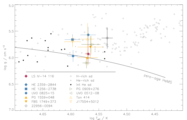
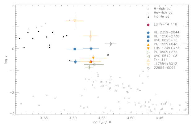
Figure 2: The distribution of heavy-metal (filled coloured symbols), helium-rich and normal hot subdwarfs with effective temperature, surface gravity (top) and surface helium-to-hydrogen ratio (bottom). In the $g-\mbox{\,$T_{\rm eff}$}$ plot, the solid line shows representative positions for the theoretical zero-age helium main-sequence (HeMS: $Z=0.02$). The observed data are from this paper (navy), Naslim et al. (2011, 2013); Jeffery et al. (2017b); Németh et al. (2012) and Wild & Jeffery (2017). Filled symbols represent heavy-metal subdwarfs.

3 Atmospheric parameters

We measured the atmospheric parameters effective temperature $T_{\rm eff}$, surface gravity $g$, and fractional helium abundance $n_{\rm He}$ of each star by fitting the observed spectrum with a grid of theoretical spectra. We used the same $\chi^{2}$-minimization method as Naslim et al. (2010, 2011); Jeffery et al. (2013); Jeffery et al. (2017b). The method compares the observed spectrum with theoretical emergent spectra computed from a grid of fully-blanketed plane-parallel model atmospheres in local thermodynamic and hydrostatic equilibrium (Behara & Jeffery, 2006) using the Armagh optimisation code sfit (Jeffery et al., 2001). sfit can use the entire observed spectrum but, by allowing the user to adjust the error associated with each datum in selected wavelength windows, can be tuned to exclude bad pixels, interstellar lines or other aggravating features. In fitting the entire blue-optical spectra of hot subdwarfs, the Stark-broadened helium and hydrogen line profiles dominate the measurement of $T_{\rm eff}$, $\log g$, and $n_{\rm He}$, although at high resolution there is a minor contribution to the $\chi^{2}$ surface from the ionization equilibria of subordinate species.

The model atmosphere grid covers the range $T_{\rm eff}=32\,000(2000)42\,000$ K, $\mbox{\,$\log g/{\rm cm\,s^{-2}}$}=5.4(0.2)6.2$ and $n_{\rm He}=0.1,0.2,0.299,0.699,0.949$ and 0.989 where parentheses represent the grid step sizes. In practice, a subset of the full grid was used in order to meet computer memory limitations; the grid subset was always adjusted iteratively to ensure that its boundaries bracketed the final solution for a given star.

Two choices were used for the distribution of elements heavier than helium in the models, namely i) m10: 1/10 solar for all $Z>2$ ($\equiv[X/{\rm H}]=-1$) and ii) sdb: 1/10 solar for $2<Z<26$ and solar for $Z\geq 26$. For two iHe-sd stars in our sample, PG 1559+048 and FBS 1749+373 which show trans-iron elements in their observed spectra, we determine the abundances and atmospheric parameters using both m10 and sdb grids for comparison. The choice of grid (m10 or sdb) made very little difference to the derived surface abundances (see § 4).

We determined $T_{\rm eff}$, $\log g$, and $n_{\rm He}$ by fitting the entire spectral region 3900–5000 Å using SFIT. We excluded the region below $<3900$Å where normalization is difficult due to blending between high-order diffuse lines in the Balmer and helium series.

Table 1 lists our measurements of $T_{\rm eff}$, $\log g$, and $n_{\rm He}$. The differences between measurements made using grids (m10 and sdb) are very small compared to the formal errors. The projected equatorial rotation velocity ( $v\,\sin i$) was measured by optimizing fits to the profiles of carbon and nitrogen lines. Table 1 also includes previous measurements of  T_eff,  log $g$ and  $n_{\rm He}$ for all four stars. These were based on low-resolution optical spectra and non-LTE model atmospheres with line blanketing due to H and He only (Thejll et al., 1994; Németh et al., 2012).

Figure 2 shows the distribution of sample stars and of other heavy-metal and chemically-peculiar subdwarfs in the $g-\mbox{\,\em T${}_{\rm eff}$}$ and $y-\mbox{\,\em T${}_{\rm eff}$}$ planes.

Formal errors in $T_{\rm eff}$ were obtained by fixing $\log g$ and $n_{\rm He}$ and fitting the spectral region 4680–4720 Å which includes the temperature sensitive He ii 4686 Å  and He i 4713 Å lines. We found formal errors in $\log g$ by fitting H${\epsilon}$, H${\delta}$ and He i 4026 Å separately while holding $T_{\rm eff}$ and $n_{\rm He}$ at fixed values.

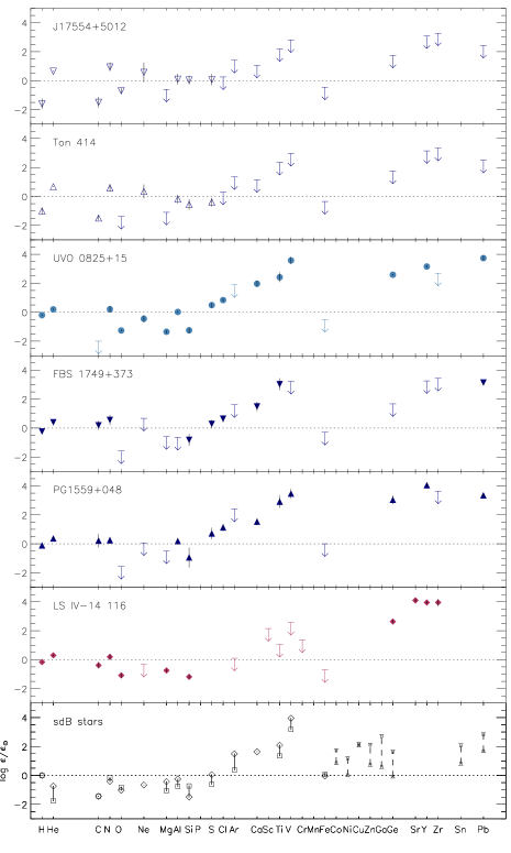
Figure 3: Surface abundances of heavy-metal subdwarfs (filled symbols), helium-rich subdwarfs (open triangles) and normal subdwarfs (bottom panel). Abundances are shown relative to solar values (dotted line). Abundance ranges for normal subdwarf B stars are shown for (i) $Z\leq 26$ (solid lines): the average abundances for cool (squares) and warm (diamonds) sdBs (Geier, 2013) and (ii) $Z\geq 27$ (broken lines): the range (delimited by hats) of abundances measured for five normal sdBs from UV spectroscopy (O’Toole & Heber, 2006).

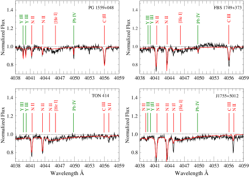
Figure 4: Locations of Pb iv 4049.48 Å, Y iii 4039.60 Å, and Y iii 4040.11 Å in the Subaru spectra of PG 1559+048, FBS 1749+373, Ton 414 and J17554+5012 along with the best fit model for each star. The Pb iv line is detected in both PG 1559+048 and FBS 1749+373. The Y iii lines are detected only in PG 1559+048. The broad depression around 4045.2 Å is due to a forbidden transition of He i ($2^{3}{\rm P}^{0}-5^{3}{\rm P}^{0}$). Spectra are plotted in the observer’s rest frame, thus include solar and stellar radial velocity shifts.

4 Abundances

We measured the equivalent widths of all C, N, O, Al, Si, S, Cl, Ca, Ti, V, Ge, Y and Pb absorption lines for which we had atomic data. Line abundances were calculated from equivalent widths using the LTE radiative transfer code spectrum (Jeffery et al., 2001). An atomic abundance is calculated from a given model atmosphere structure and a line equivalent width by Newton-Raphson iteration on the curve of growth. Individual absorption line equivalent widths and abundances are shown in Table A.3.

The mean surface abundances of measured elements in PG 1559+048, FBS 1749+373, Ton 414 and J17554+5012 are shown in Table 2 in the form $\log\epsilon_{i}=\log n_{i}+c$ where $\log\Sigma_{i}a_{i}n_{i}=12.15$ and $a_{i}$ are atomic weights. This form conserves values of $\epsilon_{i}$ for elements whose abundances do not change, even when the mean atomic mass of the mixture changes substantially.

For PG 1559+048 and FBS 1749+373, which show lines due to trans-iron elements, we determined elemental abundances using models computed with both mixtures m10 and sdb. The differences between the abundances derived using these models are negligible (Table 2). For the more helium-rich subdwarfs, Ton 414 and J17554+5012, we determined abundances using mixture m10. In all cases, we used the grid model closest to the measured $T_{\rm eff}$, $\log g$, and $n_{\rm He}$ given in Table 1. Full details of the adopted models are shown in the footnotes to Table 2 and Table A.3.

In all cases we adopted a micro-turbulent velocity $v_{\rm t}=5\,{\rm km\,s^{-1}}$. Measuring $v{\rm{}_{t}}$ in iHe-sds is difficult as it a) requires an ion with (preferably) many lines covering a large range of equivalent width and b) generally assumes the photosphere to be chemically homogeneous in the parent atom. For the iHe-sds in our sample the condition is not satisfied and the photosphere is likely to chemically stratified by radiative levitation. To test the consequences of adopting $v_{\rm t}=5\,{\rm km\,s^{-1}}$ we compared abundances for all four stars for $v_{\rm t}=0$ and $5\,{\rm km\,s^{-1}}$ and found differences negligible compared with the statistical errors (Table A.4). Reducing $v{\rm{}_{t}}$ to $0\,{\rm km\,s^{-1}}$ increases elemental abundances by between .01 and .09 dex.

The errors given in Table A.3 are standard deviations of the line abundances about the mean or, in the case of a single representative line, derived from the estimated error in the equivalent width measurement.

An additional systematic error is introduced by the errors in  T_eff and $g$. Naslim et al. (2011) obtained representative values for $\delta\epsilon_{i}/\delta\mbox{\,\em T${}_{\rm eff}$}$, $\delta\epsilon_{i}/\delta\log g$ and $\delta\epsilon_{i}/\delta v_{\rm t}$ for LS IV$-14^{\circ}116$ (ibid. Table 5). The latter are comparable with values obtained for the current sample (Table A.4). Note that  T_eff, $\log g$ and $n_{\rm He}$ are correlated. For a given spectrum, similar fits can be obtained by increasing both  log $g$ and  T_eff simultaneously since higher gravity corresponds to higher pressure in the photosphere and hence to increased ionization. Similarly, raising  $T_{\rm eff}$ requires more helium to match the Hei lines. Hence only $\delta\mbox{\,\em T${}_{\rm eff}$}$ need be considered. The abundance error due to the error in  T_eff can then be computed from $\delta\mbox{\,\em T${}_{\rm eff}$}$ in Table 1 and $\delta\epsilon_{i}/\delta\mbox{\,\em T${}_{\rm eff}$}$ from Naslim et al. (2011, Table 5), supplemented for Ne, Al, Cl, Al, Ti, V, and Pb with error gradients measured from the current data. This error should be combined quadratically with the error in Table 2 and a contribution due to the micro-turbulent velocity assumption from Table A.4. Considering yttrium in PG 1559+04, we find contributions of $\pm 0.13$, $\pm 0.10$ and $\pm 0.01$ respectively giving a total error $\delta\epsilon_{\rm Y}\approx\pm 0.16$, whilst for carbon, the same calculation gives $\pm 0.08$, $\pm 0.46$ and $\pm 0.08$ yielding $\delta\epsilon_{\rm C}\pm 0.47$. Where the abundance is derived from few lines of a single ion with small scatter, the systematics are significant. In other cases, the statistical errors dominate.

The errors given in Table 2 are the total errors derived from the quadratic sum of the statistical error and the systematic errors in  T_eff and $v_{\rm t}$.

Surface abundances relative to the Sun for the programme stars, UVO 0825$+$15 and LS IV$-14^{\circ}116$ are shown in Figure 3 where they are compared with the observed range in surface abundance seen in normal subdwarf B stars (Geier, 2013; O’Toole & Heber, 2006).

Figure 4 shows the Pb iv 4049.48 Å line in PG 1559+048 and FBS 1749+373. It also shows the Y iii 4039.60 and 4040.11 Å lines in PG 1559+048 together with the best fit model spectrum. Locations of these lines in Ton 414 and J17554+5012 are shown for comparison. In PG 1559+048 germanium is 3.0 dex overabundant, lead is 3.3 dex and yttrium is 4.0 dex overabundant, relative to solar. In FBS 1749+373, lead is 3.1 dex overabundant relative to solar. In both PG 1559+048 and FBS 1749+373 carbon and nitrogen are nearly solar or slightly over abundant, whereas oxygen, neon and aluminium are underabundant. The He-sds, Ton 414 and J17554+5012 do not show any elements heavier than sulphur. In both these stars carbon and oxygen are underabundant, while nitrogen is overabundant (0.6–0.9 dex) relative to solar. Upper limits were estimated for significant elements not seen in the spectrum by assuming the equivalent width of the strongest line due to that element in the observed spectral range to be less than 5 mÅ .

Jeffery et al. (2017b) reported over 150 unidentified absorption lines in the Subaru/HDS spectrum of UVO 0825$+$15. The majority of these lines having equivalent widths above the detection threshold of 5 mÅ  are found in the Subaru/HDS spectra of lead-rich stars PG 1559+048 and FBS 1749+373 (Figure 5). We cross checked these lines with the NIST Atomic Spectra Database; however these lines remain unidentified.

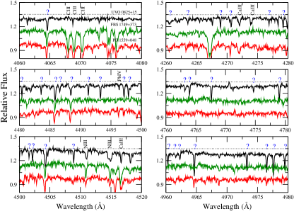
Figure 5: Unidentified lines in Subaru HDS spectra of three iHe-sd stars UVO 0825$+$15 (Jeffery et al., 2017b), FBS 1749+373 and PG 1559+048 (this paper).

5 Conclusion

Five He-sd stars were observed using the high-dispersion spectrograph on the Subaru telescope in an experiment aimed at discovering the numerical frequency of heavy-metal subdwarfs and the range in  T_eff  $g$ and $n_{\rm He}$ over which they occur. We have presented abundance analyses of two He-sd stars having helium-to-hydrogen ratio $\log y>0.5$ and two iHe-sd stars having $-1<\log y<-0.5$. The latter, PG 1559+048 and FBS 1749+373, show absorption lines due to triply ionized lead (Pb iv) and have lead abundances between 3 and 4 dex above solar. PG 1559+048 also shows germanium and yttrium (Ge iii and Y iii) with abundances comparable to those seen in LS IV$-14^{\circ}116$ (Naslim et al., 2011). An analysis of the fifth star, and the third lead-rich star, was presented by Jeffery et al. (2017b). Ton 414 and J17554+5012 do not show absorption lines due to heavy elements germanium, yttrium or lead. Our analysis confirm that J17554+5012 is a ’helium enriched’ He-sd having $\log y$= 1.27. With $\log y$= 0.58, Ton 414 is strictly an iHe-sd, but has substantially more helium than the other two stars in which heavy elements were detected.

From the sample of five stars, the three stars known to be iHe-sds (intermediate helium-rich subdwarfs) were discovered to be lead-rich. The other two were not. From this perspective it appears to be possible to predict with a relatively high level of certainty which hot subdwarfs are likely to show trans-iron elements in their optical spectra. Testing this will be pursued with continuing observations elsewhere. From there, it will be a relatively straightforward step to evaluate the numerical frequency of heavy-metal subdwarfs using data on iHe-sds from current surveys such as, for example, Gaia + LAMOST (Lei et al., 2018, 2019).

Our second goal was to explore the systematics of heavy-metal subdwarfs with regard to distribution in  T_eff, $g$, and $y$. Figure 2 demonstrates that the heavy-metal subdwarfs analyzed so far cluster in the ranges $35\,000<\mbox{\,\em T${}_{\rm eff}$}/{\rm K}<40\,000$, $6.0<\mbox{\,$\log g/{\rm cm\,s^{-2}}$}<5.5$ and $-1<\log y\mathrel{\raise 1.16pt\hbox{$<$}\kern-7.0pt\lower 3.06pt\hbox{{$\scriptstyle\sim$}}}0$. Numbers remain too small to determine where zirconium, or lead, or both are most likely to be seen.

Corollaries to this question include whether heavy-metal superabundances occur outside this region, whether abundances of trans-iron elements are elevated to a lesser extent in adjacent regions, and whether the regions includes stars with less exotic surface compositions. Addressing the first point, the two stars in the present sample which are not ‘heavy-metal’ stars have $\log y\geq 0.5$. With $\log y>1$, J17554+5012 at least is an extreme helium-rich hot subdwarf. Both are nitrogen-rich and carbon-poor. In addition, Naslim et al. (2010) analysed a sample of 5 He-sds and 1 iHe-sd with $30\,000<\mbox{\,\em T${}_{\rm eff}$}/{\rm K}<40\,000$ and $6.0<\mbox{\,$\log g/{\rm cm\,s^{-2}}$}<4.5$ without noting significant numbers of unidentified lines (ibid. Figs. A1 – A6). The spectra of these stars were rechecked following the publication of Naslim et al. (2011) and Naslim et al. (2013): no lines due to heavy elements were found. The absence of heavy metal absorption lines in Ton 414 and J17554+5012 and of optical Ge iii, Y iii and Zr iv lines in any star analyzed before their identification in LS IV$-14^{\circ}116$ argues strongly that subdwarfs with $\log y\mathrel{\raise 1.16pt\hbox{$>$}\kern-7.0pt\lower 3.06pt\hbox{{$\scriptstyle\sim$}}}0$ have not, so far, shown evidence of extreme heavy-metal overabundances. Evidence of heavy-metal enhancement by up to 2–3 dex would require high-resolution ultraviolet spectroscopy. A search for heavy-element enhancements is continuing via the SALT survey of chemically peculiar subdwarfs (Jeffery, 2017; Jeffery et al., 2017a; Jeffery & Miszalski, 2019).

Turning to other questions raised in the introduction, it is clear that whatever physics produces extreme overabundances of lead and other heavy elements must also be associated with intermediate helium enrichment. Assuming the physics responsible is selective radiative levitation and that the surface layers are initially homogeneous, a superabundance by $d$ dex of element $Z$ in a region of mass $m$ must be associated with depletion in a region of mass $\geq 10^{d}m$. This represents a significant constraint for normal helium-poor sdB stars, where germanium, tin and lead, at least, are known to be elevated above solar values by 2–3 dex (Chayer et al., 2006; O’Toole & Heber, 2006). This constraint becomes even more severe for the heavy-metal subdwarfs. Some relief can be obtained by assuming that the stellar atmosphere is heavily stratified and that the enriched layer is confined to the line forming region. Since this has direct consequences for the measurement of abundances in the photosphere, for the model atmospheres and the assumptions made in the analysis, self-consistent model atmospheres which can account for the levitation of lead and other exotic species are urgently required to test this conjecture and to deduce the overall masses of enriched and depleted material.

Broader questions relate to the origin and internal structure of the heavy-metal subdwarfs. Do they represent the high-temperature limit of the normal sdB stars in which radiative levitation has produced an extreme chemistry? Or do they originate from some other channel? Saio & Jeffery (2019) argue, for example, that LS IV$-14^{\circ}116$ represents the stripped core of a 3 $\rm M_{\odot}$ helium star. Answers to these questions will be addressed by looking at a larger ensemble of stars including other recent discoveries, and including distance and proper-motion measurements from Gaia.

Meanwhile, discoveries of other heavy-metal subdwarfs are being announced (Jeffery & Miszalski, 2019; Dorsch et al., 2019; Latour et al., 2019b). Self-consistent model atmospheres with chemical diffusion and radiative levitation which can treat these heavy elements are urgently needed. Investigations of the masses, luminosities and space motions, and of the internal structure and evolutionary status of the heavy-metal subdwarfs are also in progress.

Appendix A Spectral analysis

This appendix contains the line-by-line analysis of the Subaru/HDS spectra, including equivalent widths and derived abundances (Table A.3) and a spectral atlas for each star (Figures A.6 – A.9). Table A.4 compares abundances derived assuming a microturbulent velocity $v_{t}=0\,\mbox{$\mbox{km}\,\mbox{s}^{-1}$}$ with those presented in Table 2 assuming $v_{t}=5\,\mbox{$\mbox{km}\,\mbox{s}^{-1}$}$.

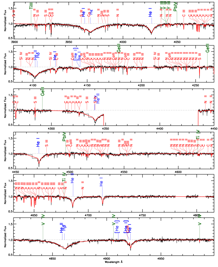
Figure A.6: The Subaru spectrum of PG 1559+048 along with the best fit model.

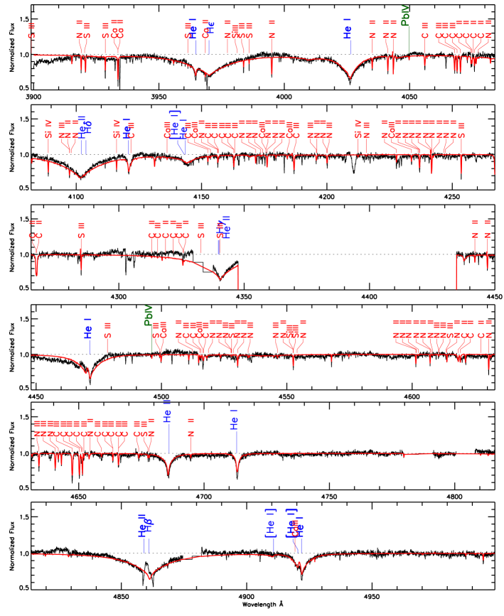
Figure A.7: The Subaru spectrum of FBS 1749+373 along with the best fit model.

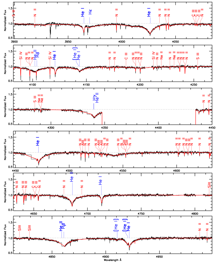
Figure A.8: The Subaru spectrum of Ton 414 along with the best fit model.

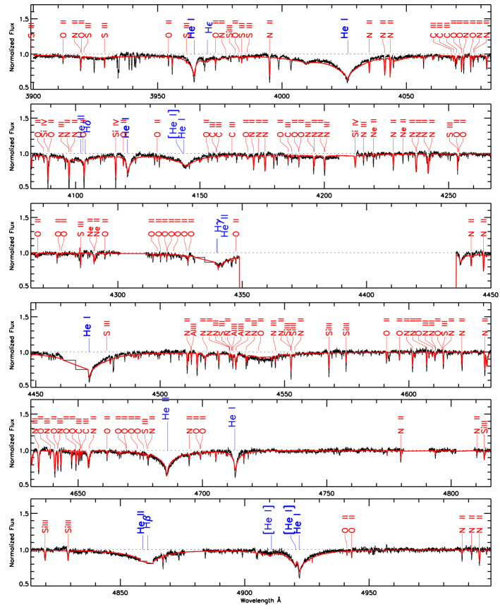
Figure A.9: The Subaru spectrum of J 1755+5012 along with the best fit model.

Table A.3: Measured equivalent width ($w_{\lambda}$) and derived abundances $\log\epsilon_{i}$ for each line. Averages and standard deviations (in parentheses) are reported for each ion. The model atmospheres and sources for $gf$-values used are reported at the end of the table.

Ion	PG 1559+048			FBS 1749+373			Ton 414		J 1755+5012
$\lambda({\rm\AA})$	$w_{\lambda}({\rm m\AA})$	${}^{a}\log\epsilon_{i}$	${}^{b}\log\epsilon_{i}$	$w_{\lambda}({\rm m\AA})$	${}^{c}\log\epsilon_{i}$	${}^{d}\log\epsilon_{i}$	$w_{\lambda}({\rm m\AA})$	${}^{e}\log\epsilon_{i}$	$w_{\lambda}({\rm m\AA})$	${}^{f}\log\epsilon_{i}$
C ii
3918.98	60	9.19	9.13	53	8.68	8.68
3920.69	72	9.03	8.98	56	8.42	8.42
4074.48$\rceil$
4074.52 $|$	85	8.99	8.94	85	8.65	8.65
4074.85$\rfloor$
4075.94$\rceil$
4075.85$\rfloor$	63	8.54	8.49	78	8.31	8.31
4267.02$\rceil$
4267.27$\rfloor$	190	8.75	8.70	230	8.52	8.53
		8.90(0.26)	8.85(0.25)		8.52(0.16)	8.52(0.16)
C iii
4067.94	76	7.78	7.80	90	8.06	8.08			11	6.38
4068.91	85	7.87	7.89	98	8.14	8.16			30	6.88
4070.26	95	8.56	8.59	120	9.07	9.10			14	6.69
4647.42	160	8.46	8.47	195	8.73	8.75	36	6.83	75	7.27
4650.25	120	8.31	8.34	146	8.60	8.63	35	7.04	48	7.14
4651.47	102	8.60	8.62	128	8.93	8.95			30	7.30
4056.05	59	8.50	8.51	77	8.80	8.82
4152.51	100	9.14	9.17	29	8.72	8.74
4156.74	100	9.31	9.34	60	8.98	9.00
		8.50(0.50)	8.52(0.51)		8.67(0.35)	8.69(0.36)		6.94(0.15)		6.94(0.36)
N ii
3995.00	34	8.00	7.96	78	8.30	8.31	70	8.17	120	8.70
4041.31	22	7.84	7.80	70	8.23	8.24	70	8.13	97	8.30
4073.05							33	8.65	57	8.90
4171.59							40	8.34	60	8.51
4176.16							42	8.05	97	8.52
4043.53	20	7.90	7.87	50	8.13	8.13	48	8.00	100	8.44
4236.98	22	8.14	8.10	90	8.73	8.74	80	8.53	140	8.91
4241.78	36	8.24	8.21	80	8.48	8.49	67	8.25	90	8.39
4447.03	30	8.25	8.22	58	8.41	8.42	62	8.43	100	8.86
4530.40							58	8.27	105	8.62
4643.09							50	8.59	97	9.16
4630.54	33	8.17	8.14	72	8.44	8.46	54	8.17	100	8.72
4621.29									95	9.23
4613.87							46	8.74	85	9.23
4601.48	18	8.30	8.27	33	8.33	8.33	50	8.58	92	9.09
4607.16							37	8.46	83	9.08
4097.33				51	7.57	7.59	120	8.16	170	8.44
		8.10(0.17)	8.07(0.17)		8.30(0.32)	8.30(0.32)		8.35(0.23)		8.77(0.31)
N iii
4640.64	77	8.09	8.14	89	8.44	8.46	130	8.53	150	8.53
4641.85							60	8.70	90	8.93
4103.43							90	8.14	150	8.60
4195.76							65	8.82	97	9.01
4200.10	38	7.61	7.65	65	8.92	8.95	76	8.70	120	8.97
4634.14	30	8.29	8.32	90	8.71	8.74	105	8.56	150	8.79
4610.55									50	9.07
4544.80							30	8.60	42	8.63
4546.32									42	8.65
		7.99(0.35)	8.03(0.35)		8.69(0.24)	8.72(0.25)		8.58(0.22)		8.80(0.20)

Table A.3: contd.

Ion	PG 1559+048			FBS 1749+373			Ton 414		J 1755+5012
$\lambda({\rm\AA})$	$w_{\lambda}({\rm m\AA})$	${}^{a}\log\epsilon_{i}$	${}^{b}\log\epsilon_{i}$	$w_{\lambda}({\rm m\AA})$	${}^{c}\log\epsilon_{i}$	${}^{d}\log\epsilon_{i}$	$w_{\lambda}({\rm m\AA})$	${}^{e}\log\epsilon_{i}$	$w_{\lambda}({\rm m\AA})$	${}^{f}\log\epsilon_{i}$
O ii
4649.14									65	8.02
4072.15									44	7.82
4069.88									45	8.01
4075.86									50	7.75
4119.21									31	7.74
4189.78									35	7.93
4590.97									37	8.01
4596.17									37	8.16
4638.85									27	8.07
4650.84									28	8.11
4661.63									35	8.17
4676.23									25	8.08
4942.99									28	8.06
										7.99(0.14)
Ne ii
4219.76							21	8.60	50	8.96
4231.60							16	8.77	41	9.16
4290.37							26	7.88	40	8.00
4290.60							26	7.88	30	7.86
								8.28(0.47)		8.50(0.66)
Al iii
4512.54	20	6.72	6.70				11	6.08	43	6.78
4529.20	24	6.56	6.54				35	6.45	32	6.32
		6.64(0.11)	6.62(0.11)					6.27(0.26)		6.55(0.33)
Si iii
4552.62	38	7.17	7.11	59	7.02	7.03	34	6.69	105	7.49
4567.82							25	6.74	116	7.81
4574.76									65	7.79
4828.96									85	7.57
4819.72									85	7.67
4813.30									50	7.48
3796.10	27	7.10	7.04	34	6.81	6.82	23	6.58	83	7.46
		7.14(0.05)	7.08(0.05)		6.92(0.15)	6.93(0.15)		6.67(0.08)		7.61(0.15)
Si iv
4088.85	35	6.08	6.08	50	6.40	6.41	100	6.90	193	7.58
4116.10	17	5.94	5.94	40	6.52	6.54	84	7.00	175	7.77
4654.14							140	7.25	185	7.31
4212.41							95	7.52	65	7.14
		6.01(0.10)	6.01(0.10)		6.46(0.08)	6.47(0.09)		7.17(0.28)		7.45(0.28)
S ii
4253.59	82	7.99	7.95	77	7.54	7.56	22	6.55	88	7.69
4284.99	62	7.96	7.93	60	7.58	7.59	20	6.80	70	7.72
4332.71	18	7.44	7.40	23	7.24	7.25
3717.78	61	7.81	7.77	50	7.32	7.32	10	6.48	25	6.89
3662.01	37	7.73	7.68	32	7.30	7.31	15	6.92	16	6.93
		7.79(0.22)	7.75(0.22)		7.40(0.15)	7.40(0.15)		6.69(0.21)		7.31(0.45)
S iii
3838.32	41	7.34	7.30	49	7.12	7.13	30	6.77	65	7.33
3837.80	32	7.86	7.82	28	7.43	7.44			20	7.19
3928.62	62	7.98	7.94	55	7.52	7.53			25	6.94
3983.77	42	7.96	7.92	46	7.68	7.68			22	7.16
3985.97	30	8.07	8.03	27	7.67	7.67			15	7.30
3631.99	61	7.92	7.89	50	7.43	7.44			20	6.68
3709.32	83	7.96	7.91	32	7.00	7.00	23	6.80	55	7.23
		7.87(0.24)	7.83(0.24)		7.40(0.26)	7.41(0.26)		6.79(0.02)		7.12(0.23)

Table A.3: contd.

Ion	PG 1559+048			FBS 1749+373
$\lambda({\rm\AA})$	$w_{\lambda}({\rm m\AA})$	${}^{a}\log\epsilon_{i}$	${}^{b}\log\epsilon_{i}$	$w_{\lambda}({\rm m\AA})$	${}^{c}\log\epsilon_{i}$	${}^{d}\log\epsilon_{i}$
Cl ii
3720.45	15	6.63	6.59	10	6.14	6.14
Ca iii
3761.61	15	7.80	7.79	20	7.91	7.91
4153.57	15	7.89	7.90	10	7.74	7.74
4184.20	24	7.87	7.88	16	7.70	7.71
4233.71	40	7.79	7.80	29	7.67	7.68
4499.88	23	7.46	7.48	24	7.57	7.58
4516.59	55	8.15	8.17	75	8.41	8.42
4919.28	10	7.96	7.97
5137.73	10	8.05	8.07
		7.87(0.21)	7.88(0.20)		7.83(0.30)	7.84(0.30)
Ti iii
3915.26	18	8.00	7.95	20	7.70	7.70
Ti iv
4618.04	10	7.39	7.42
4677.59	25	8.19	8.22	20	8.25	8.27
		7.79(0.57)	7.82(0.56)
V iv
4841.26	24	7.76	7.79
4985.64	23	7.37	7.40
5130.78	20	7.20	7.24
5146.52	15	7.27	7.31
		7.40(0.25)	7.43(0.25)
Ge iii
4178.96	23	6.53	6.46
4291.71	10	6.84	6.77
		6.69(0.22)	6.62(0.22)
Y iii
4039.60	15	6.02	6.00
4040.11	20	6.16	6.13
		6.09(0.10)	6.07(0.09)
Pb iv
3962.48	12	4.94	4.92	13	4.81	4.81
4049.48	20	5.16	5.14	19	4.97	4.97
4496.15	21	5.20	5.18
		5.10(0.14)	5.08(0.14)		4.89(0.11)	4.89(0.11)

$gf$ values were taken from the following. C ii: Yan & Seaton (1987), C iii: (Hibbert, 1976; Hardorp & Scholz, 1970), N ii: Becker & Butler (1990), N iii: Butler (1984), O ii: Becker & Butler (1988), Ne ii: Wiese et al. (1966), Al iii: Cunto et al. (1993), Si iii: Becker & Butler (1990), Si iv: Becker & Butler (1990), S ii: Wiese et al. (1969), S iii: Wiese et al. (1969), Cl ii: Rodriguez & Campos (1989), Ca iii: Kurucz (1999), Ti iii: Warner & Kirkpatrick (1969), V iv: Martin et al. (1988), Ge iii: Naslim et al. (2011), Y iii: Naslim et al. (2011), and Pb iv: Naslim et al. (2013)

Model atmospheres:

$a$: model: $T_{\rm eff}$ = 38 000 K, $\log$ g=6.0, $n_{\rm He}$=0.200, m10

$b$: model: $T_{\rm eff}$ = 38 000 K, $\log$ g=6.0, $n_{\rm He}$=0.200, sdb

$c$: model: $T_{\rm eff}$ = 36 000 K, $\log$ g=6.0, $n_{\rm He}$=0.300, m10

$d$: model: $T_{\rm eff}$ = 36 000 K, $\log$ g=6.0, $n_{\rm He}$=0.300, sdb

$e$: model: $T_{\rm eff}$ = 38 000 K, $\log$ g=6.0, $n_{\rm He}$=0.699, m10

$f$: model: $T_{\rm eff}$ = 40 000 K, $\log$ g=6.0, $n_{\rm He}$=0.949, m10

Table A.4: Comparison of abundances $\log\epsilon_{i}$ for microturbulent velocities $v_{t}=0.0$ and 5.0 km s^-1. Errors in parentheses are standard deviations about the mean.

	PG 1559+048		FBS 1749+373		Ton 414		J 1755+5012
$v_{t}/\,\mbox{$\mbox{km}\,\mbox{s}^{-1}$}$	0	5	0	5	0	5	0	5
Element	$\log\epsilon_{i}$	$\log\epsilon_{i}$	$\log\epsilon_{i}$	$\log\epsilon_{i}$	$\log\epsilon_{i}$	$\log\epsilon_{i}$	$\log\epsilon_{i}$	$\log\epsilon_{i}$
C	8.73(0.46)	8.65(0.46)	8.69(0.32)	8.62(0.30)	6.98(0.14)	6.94(0.15)	6.98(0.38)	6.94(0.36)
N	8.12(0.22)	8.08(0.22)	8.47(0.35)	8.39(0.34)	8.48(0.25)	8.42(0.25)	8.86(0.30)	8.78(0.28)
O							8.03(0.14)	7.99(0.14)
Ne					8.29(0.48)	8.28(0.47)	8.55(0.66)	8.50(0.66)
Al	6.69(0.11)	6.64(0.11)			6.30(0.28)	6.27(0.26)	6.60(0.33)	6.55(0.33)
Si	6.64(0.64)	6.57(0.65)	6.81(0.24)	6.69(0.28)	7.03(0.34)	6.95(0.33)	7.62(0.24)	7.55(0.33)
S	7.98(0.28)	7.84(0.23)	7.53(0.27)	7.40(0.21)	6.77(0.17)	6.72(0.17)	7.28(0.42)	7.19(0.32)
Cl	6.62(0.06)	6.63(0.06)	6.15(0.20)	6.14(0.20)
Ca	7.88(0.21)	7.87(0.21)	7.84(0.31)	7.83(0.30)
Ti	7.87(0.42)	7.86(0.42)	7.99(0.38)	7.98(0.38)
V	7.42(0.25)	7.40(0.25)
Ge	6.70(0.21)	6.69(0.22)
Y	6.10(0.10)	6.09(0.10)
Pb	5.12(0.15)	5.10(0.14)	4.90(0.12)	4.89(0.11)

References

- Abrahamian et al. (1990) Abrahamian H. V., Lipovetski V. A., Mickaelian A. M., Stepanian J. A., 1990, Astrofizika, 33, 213
- Ahmad & Jeffery (2005) Ahmad A., Jeffery C. S., 2005, A&A, 437, L51
- Ahmad et al. (2004) Ahmad A., Jeffery C. S., Solheim J.-E., Ostensen R., 2004, Ap&SS, 291, 435
- Asplund et al. (2009) Asplund M., Grevesse N., Sauval A. J., Scott P., 2009, ARA&A, 47, 481
- Becker & Butler (1988) Becker S. R., Butler K., 1988, A&AS, 74, 211
- Becker & Butler (1990) Becker S. R., Butler K., 1990, A&A, 235, 326
- Behara & Jeffery (2006) Behara N. T., Jeffery C. S., 2006, A&A, 451, 643
- Butler (1984) Butler K., 1984, PhD Thesis, University College London
- Chayer et al. (2006) Chayer P., Fontaine M., Fontaine G., Wesemael F., Dupuis J., 2006, Baltic Astronomy, 15, 131
- Cunto et al. (1993) Cunto W., Mendoza C., Ochsenbein F., Zeippen C. J., 1993, å, 275, L5+
- Dorsch et al. (2019) Dorsch M., Latour M., Heber U., 2019, A&A, in press
- Drilling et al. (2013) Drilling J. S., Jeffery C. S., Heber U., Moehler S., Napiwotzki R., 2013, A&A, 551, A31
- Geier (2013) Geier S., 2013, A&A, 549, A110
- Green et al. (1986) Green R. F., Schmidt M., Liebert J., 1986, ApJS, 61, 305
- Green et al. (2011) Green E. M., et al., 2011, ApJ, 734, 59
- Hardorp & Scholz (1970) Hardorp J., Scholz M., 1970, ApJS, 19, 193
- Hibbert (1976) Hibbert A., 1976, J.Phys.B, 9, 2805
- Jeffery (2011) Jeffery C. S., 2011, Information Bulletin on Variable Stars, 5964, 1
- Jeffery (2017) Jeffery C. S., 2017, MNRAS, 470, 3557
- Jeffery & Miszalski (2019) Jeffery C. S., Miszalski B., 2019, MNRAS, 489, 1481
- Jeffery et al. (2001) Jeffery C. S., Woolf V. M., Pollacco D. L., 2001, A&A, 376, 497
- Jeffery et al. (2013) Jeffery C. S., et al., 2013, MNRAS, 429, 3207
- Jeffery et al. (2017a) Jeffery C. S., Neelamkodan N., Woolf V. M., Crawford S. M., Østensen R. H., 2017a, Open Astronomy, 26, 202
- Jeffery et al. (2017b) Jeffery C. S., Baran A. S., Behara N. T., et al. 2017b, MNRAS, 465, 3101
- Kurucz (1999) Kurucz R. L., 1999, Robert L. Kurucz on-line database of observed and predicted atomic transitions
- Latour et al. (2019a) Latour M., Green E. M., Fontaine G., 2019a, A&A, 623, L12
- Latour et al. (2019b) Latour M., Dorsch M., Heber U., 2019b, A&A, in press
- Lei et al. (2018) Lei Z., Zhao J., Németh P., Zhao G., 2018, ApJ, 868, 70
- Lei et al. (2019) Lei Z., Zhao J., Németh P., Zhao G., 2019, arXiv e-prints, p. arXiv:1907.00128
- Martin et al. (1988) Martin G., Fuhr J., Wiese W., 1988, J. Phys. Chem. Ref. Data Suppl., 17
- Martin et al. (2017) Martin P., Jeffery C. S., Naslim N., Woolf V. M., 2017, MNRAS, 467, 68
- Mickaelian (2008) Mickaelian A. M., 2008, AJ, 136, 946
- Naslim et al. (2010) Naslim N., Jeffery C. S., Ahmad A., Behara N. T., Şahìn T., 2010, MNRAS, 409, 582
- Naslim et al. (2011) Naslim N., Jeffery C. S., Behara N. T., Hibbert A., 2011, MNRAS, 412, 363
- Naslim et al. (2013) Naslim N., Jeffery C. S., Hibbert A., Behara N. T., 2013, MNRAS, 434, 1920
- Németh et al. (2012) Németh P., Kawka A., Vennes S., 2012, MNRAS, 427, 2180
- O’Toole & Heber (2006) O’Toole S. J., Heber U., 2006, A&A, 452, 579
- Rodriguez & Campos (1989) Rodriguez L. F., Campos J., 1989, J.Quant.Spectrosc.Radiat.Transfer, 41, 377
- Saio & Jeffery (2019) Saio H., Jeffery C. S., 2019, MNRAS, 482, 758
- Thejll et al. (1994) Thejll P., Bauer F., Saffer R., Liebert J., Kunze D., Shipman H. L., 1994, ApJ, 433, 819
- Warner & Kirkpatrick (1969) Warner B., Kirkpatrick R., 1969, MNRAS, 144, 397
- Wiese et al. (1966) Wiese W. L., Smith M. W., Glennon B. M., 1966, Atomic transition probabilities. Vol. 1: Hydrogen through Neon. A critical data compilation
- Wiese et al. (1969) Wiese W. L., Smith M. W., Miles B. M., 1969, Atomic transition probabilities. Vol. 2: Sodium through Calcium. A critical data compilation
- Wild & Jeffery (2017) Wild J., Jeffery C. S., 2017, Open Astronomy, 26, 246
- Yan & Seaton (1987) Yan Y., Seaton M. J., 1987, Journal of Physics B Atomic Molecular Physics, 20, 6409