Learning GANs and Ensembles Using Discrepancy

Abstract

Generative adversarial networks (GANs) generate data based on minimizing a divergence between two distributions. The choice of that divergence is therefore critical. We argue that the divergence must take into account the hypothesis set and the loss function used in a subsequent learning task, where the data generated by a GAN serves for training. Taking that structural information into account is also important to derive generalization guarantees. Thus, we propose to use the discrepancy measure, which was originally introduced for the closely related problem of domain adaptation and which precisely takes into account the hypothesis set and the loss function. We show that discrepancy admits favorable properties for training GANs and prove explicit generalization guarantees. We present efficient algorithms using discrepancy for two tasks: training a GAN directly, namely DGAN, and mixing previously trained generative models, namely EDGAN. Our experiments on toy examples and several benchmark datasets show that DGAN is competitive with other GANs and that EDGAN outperforms existing GAN ensembles, such as AdaGAN.

1 Introduction

Generative adversarial networks (GANs) consist of a family of methods for unsupervised learning. A GAN learns a generative model that can easily output samples following a distribution $\mathbb{P}_{\theta}$, which aims to mimic the real data distribution $\mathbb{P}_{r}$. The parameter $\theta$ of the generator is learned by minimizing a divergence between $\mathbb{P}_{r}$ and $\mathbb{P}_{\theta}$, and different choices of this divergence lead to different GAN algorithms: the Jensen-Shannon divergence gives the standard GAN (Goodfellow et al., 2014; Salimans et al., 2016), the Wasserstein distance gives the WGAN (Arjovsky et al., 2017; Gulrajani et al., 2017), the squared maximum mean discrepancy gives the MMD GAN (Li et al., 2015; Dziugaite et al., 2015; Li et al., 2017), and the $f$-divergence gives the $f$-GAN (Nowozin et al., 2016), just to name a few. There are many other GANs that have been derived using other divergences in the past, see (Goodfellow, 2017) and (Creswell et al., 2018) for more extensive studies.

The choice of the divergence seems to be critical in the design of a GAN. But, how should that divergence be selected or defined? We argue that its choice must take into consideration the structure of a learning task and include, in particular, the hypothesis set and the loss function considered. In contrast, divergences that ignore the hypothesis set typically cannot benefit from any generalization guarantee (see for example Arora et al. (2017)). The loss function is also crucial: while many GAN applications aim to generate synthetic samples indistinguishable from original ones, for example images (Karras et al., 2018; Brock et al., 2019) or Anime characters (Jin et al., 2017), in many other applications, the generated samples are used to improve subsequent learning tasks, such as data augmentation (Frid-Adar et al., 2018), improved anomaly detection (Zenati et al., 2018), or model compression (Liu et al., 2018b). Such subsequent learning tasks require optimizing a specific loss function applied to the data. Thus, it would seem beneficial to explicitly incorporate this loss in the training of a GAN.

A natural divergence that accounts for both the loss function and the hypothesis set is the discrepancy measure introduced by Mansour et al. (2009). Discrepancy plays a key role in the analysis of domain adaptation, which is closely related to the GAN problem, and other related problems such as drifting and time series prediction (Mohri and Medina, 2012; Kuznetsov and Mohri, 2015). Several important generalization bounds for domain adaptation are expressed in terms of discrepancy (Mansour et al., 2009; Cortes and Mohri, 2014; Ben-David et al., 2007). We define discrepancy in Section 2 and give examples illustrating the benefit of using discrepancy to measure the divergence between distributions.

In this work, we design a new GAN technique, discrepancy GAN (DGAN), that minimizes the discrepancy between $\mathbb{P}_{\theta}$ and $\mathbb{P}_{r}$. By training GANs with discrepancy, we obtain theoretical guarantees for subsequent learning tasks using the samples it generates. We show that discrepancy is continuous with respect to the generator’s parameter $\theta$, under mild conditions, which makes training DGAN easy. Another key property of the discrepancy is that it can be accurately estimated from finite samples when the hypothesis set admits bounded complexity. This property does not hold for popular metrics such as the Jensen-Shannon divergence and the Wasserstein distance.

Moreover, we propose to use discrepancy to learn an ensemble of pre-trained GANs, which results in our EDGAN algorithm. By considering an ensemble of GANs, one can greatly reduce the problem of missing modes that frequently occurs when training a single GAN. We show that the discrepancy between the true and the ensemble distribution learned on finite samples converges to the discrepancy between the true and the optimal ensemble distribution, as the sample size increases. We also show that the EDGAN problem can be formulated as a convex optimization problem, thereby benefiting from strong convergence guarantees. Recent work of Tolstikhin et al. (2017), Arora et al. (2017), Ghosh et al. (2018) and Hoang et al. (2018) also considered mixing GANs, either motived by boosting algorithms such as AdaBoost, or by the minimax theorem in game theory. These algorithms train multiple generators and learn the mixture weights simultaneously, yet none of them explicitly optimizes for the mixture weights once the multiple GANs are learned, which can provide additional improvement as demonstrated by our experiments with EDGAN.

The term “discrepancy” has been previously used in the GAN literature under a different definition. The squared maximum mean discrepancy (MMD), which was originally proposed by Gretton et al. (2012), is used as the distance metric for training MMD GAN (Li et al., 2015; Dziugaite et al., 2015; Li et al., 2017). MMD between two distributions is defined with respect to a family of functions $\mathcal{F}$, which is usually assumed to be a reproducing kernel Hilbert space (RKHS) induced by a kernel function, but MMD does not take into account the loss function. LSGAN (Mao et al., 2017) also adopts the squared loss function for the discriminator, and as we do for DGAN. Feizi et al. (2017); Deshpande et al. (2018) consider minimizing the quadratic Wasserstein distance between the true and the generated samples, which involves the squared loss function as well. However, their training objectives are vastly different from ours. Finally, when the hypothesis set is the family of linear functions with bounded norm and the loss function is the squared loss, DGAN coincides with the objective sought by McGAN (Mroueh et al., 2017), that of matching the empirical covariance matrices of the true and the generated distribution. However, McGAN uses nuclear norm while DGAN uses spectral norm in that case.

The rest of this paper is organized as follows. In Section 2, we define discrepancy and prove that it benefits from several favorable properties, including continuity with respect to the generator’s parameter and the possibility of accurately estimating it from finite samples. In Section 3, we describe our discrepancy GAN (DGAN) and ensemble discrepancy GAN (EDGAN) algorithms with a discussion of the optimization solution and theoretical guarantees. We report the results of a series of experiments (Section 4), on both toy examples and several benchmark datasets, showing that DGAN is competitive with other GANs and that EDGAN outperforms existing GAN ensembles, such as AdaGAN.

2 Discrepancy

Let $\mathbb{P}_{r}$ denote the real data distribution on $\mathcal{X}$, which, without loss of generality, we can assume to be $\mathcal{X}=\{x\in\mathbb{R}^{d}\colon\|x\|_{2}\leq 1\}$. A GAN generates a sample in $\mathcal{X}$ via the following procedure: it first draws a random noise vector $z\in\mathcal{Z}$ from a fixed distribution $\mathbb{P}_{z}$, typically a multivariate Gaussian, and then passes $z$ through the generator $g_{\theta}\colon\mathcal{Z}\to\mathcal{X}$, typically a neural network parametrized by $\theta\in\Theta$. Let $\mathbb{P}_{\theta}$ denote the resulting distribution of $g_{\theta}(z)$. Given a distance metric $d(\cdot,\cdot)$ between two distributions, a GAN’s learning objective is to minimize $d(\mathbb{P}_{r},\mathbb{P}_{\theta})$ over $\theta\in\Theta$.

In Appendix A, we present and discuss two instances of the distance metric $d(\cdot,\cdot)$ and two widely-used GANs: the Jensen-Shannon divergence for the standard GAN (Goodfellow et al., 2014), and the Wasserstein distance for WGAN (Arjovsky et al., 2017). Furthermore, we show that Wasserstein distance can be viewed as discrepancy without considering the hypothesis set and the loss function, which is one of the reasons why it cannot benefit from theoretical guarantees. In this section, we describe the discrepancy measure and motivate its use by showing that it benefits from several important favorable properties.

Consider a hypothesis set $\mathcal{H}$ and a symmetric loss function $\ell\colon\mathcal{Y}\times\mathcal{Y}\to\mathbb{R}$, which will be used in future supervised learning tasks on the true (and probably also the generated) data. Given $\mathcal{H}$ and $\ell$, the discrepancy between two distributions $\mathbb{P}$ and $\mathbb{Q}$ is defined by the following:

$$\text{disc}_{\mathcal{H},\ell}(\mathbb{P},\mathbb{Q})=\sup_{h,h^{\prime}\in\mathcal{H}}\Big{|}\operatorname*{\mathbb{E}}_{x\sim\mathbb{P}}\big{[}\ell\big{(}h(x),h^{\prime}(x)\big{)}\big{]}-\operatorname*{\mathbb{E}}_{x\sim\mathbb{Q}}\big{[}\ell\big{(}h(x),h^{\prime}(x)\big{)}\big{]}\Big{|}.$$ (1)

Equivalently, let $\ell_{\mathcal{H}}=\big{\{}\ell\big{(}h(x),h^{\prime}(x)\big{)}\colon h,h^{\prime}\in\mathcal{H}\big{\}}$ be the family of discriminators induced by $\ell$ and $\mathcal{H}$, then, the discrepancy can be written as $\text{disc}_{\mathcal{H},\ell}(\mathbb{P},\mathbb{Q})=\sup_{f\in\ell_{\mathcal{H}}}\big{|}\operatorname*{\mathbb{E}}_{\mathbb{P}}[f(x)]-\operatorname*{\mathbb{E}}_{\mathbb{Q}}[f(x)]\big{|}$.

How would subsequent learning tasks benefit from samples generated by GANs trained with discrepancy? We show that, under mild conditions, any hypothesis performing well on $\mathbb{P}_{\theta}$ (with loss function $\ell$) is guaranteed to perform well on $\mathbb{P}_{r}$, as long as the discrepancy $\text{disc}_{\mathcal{H},\ell}(\mathbb{P}_{\theta},\mathbb{P}_{r})$ is small.

Theorem 1.

Assume the true labeling function $f\colon\mathcal{X}\to\mathcal{Y}$ is contained in the hypothesis set $\mathcal{H}$. Then, for any hypothesis $h\in\mathcal{H}$,

$$\operatorname*{\mathbb{E}}_{x\sim\mathbb{P}_{r}}[\ell(h,f)]\leq\operatorname*{\mathbb{E}}_{x\sim\mathbb{P}_{\theta}}[\ell(h,f)]+\text{disc}_{\mathcal{H},\ell}(\mathbb{P}_{\theta},\mathbb{P}_{r}).$$

Theorem 1 suggests that the learner can learn a model using samples drawn from $\mathbb{P}_{\theta}$, whose generation error on $\mathbb{P}_{r}$ is guaranteed to be no more than its generation error on $\mathbb{P}_{\theta}$ plus the discrepancy, which is minimized by the algorithm. The proof uses the definition of discrepancy. Due to space limitation, we provide all the proofs in Appendix B.

2.1 Hypothesis set and loss function

We argue that discrepancy is more favorable than Wasserstein distance measures, since it makes explicit the dependence on loss function and hypothesis set. We consider two widely used learning scenarios: 0-1 loss with linear separators, and squared loss with Lipschitz functions.

0-1 Loss, Linear Separators

Consider the two distributions on $\mathbb{R}^{2}$ illustrated in Figure 1(a): $\mathbb{Q}$ (filled circles $\bullet$) is equivalent to $\mathbb{P}$ (circles $\circ$), but with all points shifted to the right by a small amount $\epsilon$. Then, by the definition of Wasserstein distance, $W(\mathbb{P},\mathbb{Q})=\epsilon$, since to transport $\mathbb{P}$ to $\mathbb{Q}$, one just need to move each point to the right by $\epsilon$. When $\epsilon$ is small, WGAN views the two distributions as close and thus stops training. On the other hand, when $\ell$ is the 0-1 loss and $\mathcal{H}$ is the set of linear separators, $\text{disc}_{\mathcal{H},\ell}(\mathbb{P},\mathbb{Q})=1$, which is achieved at the $h,h^{\prime}$ as shown in Figure 1(a), with $\operatorname*{\mathbb{E}}_{\mathbb{P}}[1_{h(x)\neq h^{\prime}(x)}]=1$ and $\operatorname*{\mathbb{E}}_{\mathbb{Q}}[1_{h(x)\neq h^{\prime}(x)}]=0$. Thus, DGAN continues training to push $\mathbb{Q}$ towards $\mathbb{P}$.

The example above is an extreme case where $\mathbb{P}$ and $\mathbb{Q}$ are separable. In more practical scenarios, the domain of the two distributions may overlap significantly, as illustrated in Figure 1(b), where $\mathbb{P}$ is in red and $\mathbb{Q}$ is in blue, and the shaded areas contain 95% probably mass. Again, $\mathbb{Q}$ equals $\mathbb{P}$ shifting to the right by $\epsilon$ and thus $W(\mathbb{P},\mathbb{Q})=\epsilon$. Since the non-overlapping area has a sizable probability mass, the discrepancy between $\mathbb{P}$ and $\mathbb{Q}$ is still large, for the same reason as for Figure 1(a).

These examples demonstrate the importance of taking hypothesis sets and loss functions into account when comparing two distributions: even though two distributions appear geometrically “close” under Wasserstein distance, a classifier trained on one distribution may perform poorly on another distribution. According to Theorem 1, such unfortunate behaviors are less likely to happen with $\text{disc}_{\mathcal{H},\ell}$.

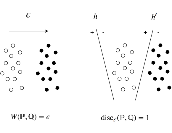
(a) Non-overlapping distributions, $\mathbb{P}$: $\{\circ\}$, $\mathbb{Q}$: $\{\bullet\}$.

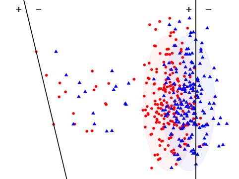
(b) Overlapping distributions, $\mathbb{P}$: $\{{\color[rgb]{1,0,0}\text{red}}\}$, $\mathbb{Q}$: $\{{\color[rgb]{0,0,1}\text{blue}}\}$.

Figure 1: Distributions $\mathbb{P}$ and $\mathbb{Q}$ may appear “close” under Wasserstein distance, but the discrepancy between the two is still large, where the discrepancy is defined by 0-1 loss and linear separators.

Squared Loss, Lipschitz Functions

Next, we consider the squared loss and the hypothesis set of 1-Lipschitz functions $\mathcal{H}=\{h\colon|h(x)-h(x^{\prime})|\leq\|x-x^{\prime}\|_{2},\forall x,x^{\prime}\in\mathcal{X}\}$, then $\ell_{\mathcal{H}}=\{[h(x)-h^{\prime}(x)]^{2}\colon h,h^{\prime}\in\mathcal{H}\}$. We can show that $\ell_{\mathcal{H}}$ is a subset of 4-Lipschitz functions on $\mathcal{X}$. Then, by the definition of discrepancy and Wasserstein distance, $\text{disc}_{\mathcal{H},\ell}(\mathbb{P},\mathbb{Q})$ is comparable to $W(\mathbb{P},\mathbb{Q})$:

$$\text{disc}_{\mathcal{H},\ell}(\mathbb{P},\mathbb{Q})=\sup_{f\in\ell_{\mathcal{H}}}\operatorname*{\mathbb{E}}_{\mathbb{P}}\big{[}f(x)\big{]}-\operatorname*{\mathbb{E}}_{\mathbb{Q}}\big{[}f(x)\big{]}\leq\sup_{f\colon 4\text{-Lipschitz}}\operatorname*{\mathbb{E}}_{\mathbb{P}}\big{[}f(x)\big{]}-\operatorname*{\mathbb{E}}_{\mathbb{Q}}\big{[}f(x)\big{]}=4W(\mathbb{P},\mathbb{Q}).$$

However, the inequality above can be quite loose since, depending on the hypothesis set, $\ell_{\mathcal{H}}$ may be only a small subset of all $4$-Lipschitz functions. For instance, when $\mathcal{H}$ is the set of linear functions with norm bounded by one, then $\ell_{\mathcal{H}}=\{(w^{T}x)^{2}\colon\|w\|\leq 2\}$, which is a significantly smaller set than the family of all $4$-Lipschitz functions. Thus, $\text{disc}_{\mathcal{H},\ell}(\mathbb{P},\mathbb{Q})$ could potentially be a tighter measure than $W(\mathbb{P},\mathbb{Q})$, depending on $\mathcal{H}$.

2.2 Continuity and estimation

In this section, we discuss two favorable properties of discrepancy: its continuity under mild assumptions with respect to the generator’s parameter $\theta$, a property shared with the Wasserstein distance, and the fact that it can be accurately estimated from finite samples, which does not hold for either the Jensen-Shannon or the Wasserstein distance. The continuity property is summarized in the following theorem.

Theorem 2.

Let $\mathcal{H}=\{h\colon\mathcal{X}\to\mathcal{Y}\}$ be a family of $\mu$-Lipschitz functions and assume that the loss function $\ell$ is continuous and symmetric in its arguments, and is bounded by $M$. Assume further that $\ell$ admits the triangle inequality, or that it can be written as $\ell(y,y^{\prime})=f(|y-y^{\prime}|)$ for some Lipschitz function $f$. Assume that $g_{\theta}\colon\mathcal{Z}\to\mathcal{X}$ is continuous in $\theta$. Then, $\text{disc}_{\mathcal{H},\ell}(\mathbb{P}_{r},\mathbb{P}_{\theta})$ is continuous in $\theta$.

The assumptions of Theorem 2 are easily satisfied in practice, where $h\in\mathcal{H}$ and $g_{\theta}$ are neural networks whose parameters are limited within a compact set, and where the loss function can be either the $\ell_{1}$ loss, $\ell(y,y^{\prime})=|y-y^{\prime}|$, or the squared loss, $\ell(y,y^{\prime})=(y-y^{\prime})^{2}$. If the discrepancy is continuous in $\theta$, then, as the sequence of parameters $\theta_{t}$ converges to $\theta^{*}$, the discrepancy also converges: $|\text{disc}_{\mathcal{H},\ell}(\mathbb{P}_{r},\mathbb{P}_{\theta_{t}})-\text{disc}_{\mathcal{H},\ell}(\mathbb{P}_{r},\mathbb{P}_{\theta^{*}})|\to 0$, which is a desirable property for training DGAN. The reader is referred to Arjovsky et al. (2017) for a more extensive discussion of the continuity properties of various distance metrics and their effects on training GANs.

Next, we show that discrepancy can be accurately estimated from finite samples. Let $S_{r}$ and $S_{\theta}$ be i.i.d. samples drawn from $\mathbb{P}_{r}$ and $\mathbb{P}_{\theta}$ with $|S_{r}|=m$ and $|S_{\theta}|=n$, and let $\widehat{\mathbb{P}}_{r}$ and $\widehat{\mathbb{P}}_{\theta}$ be the empirical distributions induced by $S_{r}$ and $S_{\theta}$, respectively. Recall that the empirical Radmacher complexity of a hypothesis set $\mathcal{G}$ on sample $S$ of size $m$ is defined by: $\widehat{\mathfrak{R}}_{S}(\mathcal{G})=\frac{2}{m}\operatorname*{\mathbb{E}}_{\sigma}\big{[}\sup_{g\in\mathcal{G}}\sum_{i=1}^{m}\sigma_{i}g(x_{i})\big{]}$, where $\sigma_{1},\sigma_{2},\dots,\sigma_{m}$ are i.i.d. random variables with $\mathbb{P}(\sigma_{i}=1)=\mathbb{P}(\sigma_{i}=-1)=1/2$. The empirical Radmacher complexity measures the complexity of the hypothesis set $\mathcal{G}$. The next theorem presents the learning guarantees of discrepancy.

Theorem 3.

Assume the loss is bounded, $\ell\leq M$. For any $\delta>0$, with probability at least $1-\delta$ over the draw of $S_{r}$ and $S_{\theta}$,

$$\big{|}\text{disc}_{\mathcal{H},\ell}(\mathbb{P}_{r},\mathbb{P}_{\theta})-\text{disc}_{\mathcal{H},\ell}(\widehat{\mathbb{P}}_{r},\widehat{\mathbb{P}}_{\theta})\big{|}\leq\widehat{\mathfrak{R}}_{S_{r}}(\ell_{\mathcal{H}})+\widehat{\mathfrak{R}}_{S_{\theta}}(\ell_{\mathcal{H}})+3M\Big{(}\sqrt{\tfrac{\log(4/\delta)}{2m}}+\sqrt{\tfrac{\log(4/\delta)}{2n}}\,\Big{)}.$$

Furthermore, when the loss function $\ell(h,h^{\prime})$ is a $q$-Lipschitz function of $h-h^{\prime}$, we have

$$\big{|}\text{disc}_{\mathcal{H},\ell}(\mathbb{P}_{r},\mathbb{P}_{\theta})-\text{disc}_{\mathcal{H},\ell}(\widehat{\mathbb{P}}_{r},\widehat{\mathbb{P}}_{\theta})\big{|}\leq 4q\Big{(}\widehat{\mathfrak{R}}_{S_{r}}(\mathcal{H})+\widehat{\mathfrak{R}}_{S_{\theta}}(\mathcal{H})\Big{)}+3M\Big{(}\sqrt{\tfrac{\log(4/\delta)}{2m}}+\sqrt{\tfrac{\log(4/\delta)}{2n}}\Big{)}.$$

In the rest of this paper, we will consider the squared loss $\ell(y,y^{\prime})=(y-y^{\prime})^{2}$, which is bounded and $2$-Lipschitz when $|h(x)|\leq 1$ for all $h\in\mathcal{H}$ and $x\in\mathcal{X}$. Furthermore, when $\mathcal{H}$ is a family of feedforward neural networks, Cortes et al. (2017) provided an explicit upper bound of $\widehat{\mathfrak{R}}_{S}(\mathcal{H})=O(1/\sqrt{m})$ for its complexity, and thus the right-hand side of the above inequality is in $O(\frac{1}{\sqrt{m}}+\frac{1}{\sqrt{n}})$. Then, for $m$ and $n$ sufficiently large, the empirical discrepancy is close to the true discrepancy. It is important that the discrepancy can be accurately estimated from finite samples since, when training DGAN, we can only approximate the true discrepancy with a batch of samples. In contrast, the Jensen-Shannon distance and the Wasserstein distance do not admit this favorable property (Arora et al., 2017).

3 Algorithms

In this section, we show how to compute the discrepancy and train DGAN for various hypothesis sets and the squared loss. We also propose to learn an ensemble of pre-trained GANs via minimizing discrepancy. We name this method EDGAN, and present its learning guarantees.

3.1 DGAN algorithm

Given a parametric family of hypotheses $\mathcal{H}=\{h_{w}\colon w\in W\}$, DGAN is defined as the following min-max optimization problem:

$$\min_{\theta\in\Theta}\max_{w,w^{\prime}\in W}\Big{|}\operatorname*{\mathbb{E}}_{x\sim\mathbb{P}_{r}}\big{[}\ell\big{(}h_{w}(x),h_{w^{\prime}}(x)\big{)}\big{]}-\operatorname*{\mathbb{E}}_{x\sim\mathbb{P}_{\theta}}\big{[}\ell\big{(}h_{w}(x),h_{w^{\prime}}(x)\big{)}\big{]}\Big{|}.$$ (2)

As with other GANs, DGAN is trained by iteratively solving the min-max problem (2). The minimization over the generator’s parameters $\theta$ can be tackled by standard stochastic gradient descent (SGD) algorithm with back-propagation. The inner maximization problem that computes the discrepancy, however, can be efficiently solved when $\ell$ is the squared loss function.

We first consider $\mathcal{H}$ to be the set of linear functions with bounded norm: $\mathcal{H}=\{x\to w^{T}x\colon\|w\|_{2}\leq 1,w\in\mathbb{R}^{{d}}\}$. Recall the definition of $S_{r}$, $S_{\theta}$, $\mathbb{P}_{r}$ and $\mathbb{P}_{\theta}$ from Section 2.2. In addition, let $X_{r}$ and $X_{\theta}$ denote the corresponding $m\times d$ and $n\times d$ data matrices, where each row represents one input.

Proposition 4.

When $\ell$ is the squared loss and $\mathcal{H}$ the family of linear functions with norm bounded by $1$, $\text{disc}_{\mathcal{H},\ell}(\widehat{\mathbb{P}}_{r},\widehat{\mathbb{P}}_{\theta})=2\left\|\frac{1}{n}X_{\theta}^{T}X_{\theta}-\frac{1}{m}X_{r}^{T}X_{r}\right\|_{2}$, where $\|\cdot\|_{2}$ denotes the spectral norm.

Thus, the discrepancy $\text{disc}_{\mathcal{H},\ell}(\widehat{\mathbb{P}}_{r},\widehat{\mathbb{P}}_{\theta})$ equals twice the largest eigenvalue in absolute value of the data-dependent matrix $\boldsymbol{M}(\theta)=\frac{1}{n}X_{\theta}^{T}X_{\theta}-\frac{1}{m}X_{r}^{T}X_{r}$. Given $v^{*}(\theta)$, the corresponding eigenvector at the optimal solution, we can then back-propagate the loss $\text{disc}_{\mathcal{H},\ell}(\widehat{\mathbb{P}}_{r},\widehat{\mathbb{P}}_{\theta})=2v^{*T}(\theta)\boldsymbol{M}(\theta)v^{*}(\theta)$ to optimize for $\theta$. The maximum or minimum eigenvalue of $\boldsymbol{M}(\theta)$ can be computed in $O(d^{2})$ (Golub and van Van Loan, 1996), and the power method can be used to closely approximate it.

The closed-form solution in Proposition 4 holds for a family $\mathcal{H}$ of linear mappings. To generate realistic outcomes with DGAN, however, we need a more complex hypothesis set $\mathcal{H}$, such as the family of deep neural networks (DNN). Thus, we consider the following approach: first, we fix a pre-trained DNN classifier, such as the inception network, and pass the samples through this network to obtain the last (or any other) layer of embedding $f\colon\mathcal{X}\to\mathcal{E}$, where $\mathcal{E}$ is the embedding space. Next, we compute the discrepancy on the embedded samples with $\mathcal{H}$ being the family of linear functions with bounded norm, which admits a closed-form solution according to Proposition 4. In practice, it also makes sense to train the embedding network together with the generator: let $f_{\zeta}$ be the embedding network parametrized by $\zeta$, then DGAN optimizes for both $f_{\zeta}$ and $g_{\theta}$ . See Algorithm 1 for a single step of updating DGAN. In particular, the learner can either compute $F(\zeta^{t},\theta^{t})$ exactly, or use an approximation based on the power method. Note that when the learner uses a pre-fixed embedding network $f$, the update step of $\zeta^{t+1}$ can be skipped.

Algorithm 1 Update DGAN(${\zeta^{t}},{\theta^{t}},\eta$)

  $X_{r}\leftarrow[f_{\zeta^{t}}(x_{1}),\cdots,f_{\zeta^{t}}(x_{m})]^{T}$, where $x_{i}\sim\mathbb{P}_{r}$

  $X_{\theta}\leftarrow[f_{\zeta^{t}}(x^{\prime}_{1}),\cdots,f_{\zeta^{t}}(x^{\prime}_{n})]^{T}$, where $x^{\prime}_{i}\sim\mathbb{P}_{\theta^{t}}$

  $F(\zeta^{t},\theta^{t})\leftarrow\left\|\frac{1}{n}X_{\theta}^{T}X_{\theta}-\frac{1}{m}X_{r}^{T}X_{r}\right\|_{2}$

  Update: $\zeta^{t+1}\leftarrow\zeta^{t}+\eta\nabla_{\zeta}F(\zeta^{t},\theta^{t})$

  Update: $\theta^{t+1}\leftarrow\theta^{t}-\eta\nabla_{\theta}F(\zeta^{t},\theta^{t})$

Algorithm 2 Update EDGAN(${\boldsymbol{\alpha}^{t}},f,\eta$)

  $X_{r}\leftarrow[f(x_{1}),\cdots,f(x_{n_{r}})]^{T}$, where $x_{i}\sim\mathbb{P}_{r}$

  $X_{k}\leftarrow[f(x^{k}_{1}),\cdots,f(x^{k}_{n_{k}})]^{T}$, where $x^{k}_{i}\sim\mathbb{P}_{\theta_{k}}$

  $F(\boldsymbol{\alpha}^{t})\leftarrow\|\big{(}\sum_{k=1}^{p}\frac{\boldsymbol{\alpha}^{t}_{k}}{n_{k}}X_{k}^{T}X_{k}\big{)}-\frac{1}{n_{r}}X_{r}^{T}X_{r}\|_{2}$

  Update: $\boldsymbol{\alpha}^{t+1}\leftarrow\boldsymbol{\alpha}^{t}-\eta\nabla_{\boldsymbol{\alpha}}F(\boldsymbol{\alpha}^{t})$

3.2 EDGAN algorithm

Next, we show that discrepancy provides a principled way of choosing the ensemble weights to mix pre-trained GANs, which admits favorable convergence guarantees.

Let $g_{1},\ldots,g_{p}$ be $p$ pre-trained GANs. For a given mixture weight $\boldsymbol{\alpha}=(\alpha_{1},\ldots,\alpha_{p})\in\Delta$, where $\Delta=\{(\alpha_{1},\ldots,\alpha_{p})\colon\alpha_{k}\geq 0,\sum_{k=1}^{p}\alpha_{k}=1\}$ is the simplex in $\mathbb{R}^{p}$, we define the ensemble of $p$ GANs by $g_{\boldsymbol{\alpha}}=\sum_{k=1}^{p}\alpha_{k}g_{k}$. To draw a sample from the ensemble $g_{\boldsymbol{\alpha}}$, we first sample an index $k\in[p]=\{1,2,\cdots,p\}$ according to the multinomial distribution with parameter $\boldsymbol{\alpha}$, and then return a random sample generated by the chosen GAN $g_{k}$. We denote by ${\mathbb{P}}_{\boldsymbol{\alpha}}$ the distribution of $g_{\boldsymbol{\alpha}}$. EDGAN determines the mixture weight $\boldsymbol{\alpha}$ by minimizing the discrepancy between ${\mathbb{P}}_{\boldsymbol{\alpha}}$ and the real data $\mathbb{P}_{r}$: $\min_{\boldsymbol{\alpha}\in\Delta}\text{disc}_{\mathcal{H},\ell}({\mathbb{P}}_{\boldsymbol{\alpha}},\mathbb{P}_{r})$.

To learn the mixture weight $\boldsymbol{\alpha}$, we approximate the true distributions by their empirical counterparts: for each $k\in[p]$, we randomly draw a set of $n_{k}$ samples from $g_{k}$, and randomly draw $n_{r}$ samples from the real data distribution $\mathbb{P}_{r}$. Let $S_{k}$ and $S_{r}$ denote the corresponding set of samples, and let $\widehat{\mathbb{P}}_{k}$ and $\widehat{\mathbb{P}}_{r}$ denote the induced empirical distributions, respectively. For a given $\boldsymbol{\alpha}$, let $\widehat{\mathbb{P}}_{\boldsymbol{\alpha}}=\sum_{k=1}^{p}\alpha_{k}\widehat{\mathbb{P}}_{k}$ be the empirical counterparts of ${\mathbb{P}}_{\boldsymbol{\alpha}}$. We first present a convergence result for the EDGAN method, and then describe how to train EDGAN.

Let $\boldsymbol{\alpha}^{*}$ and $\widehat{\boldsymbol{\alpha}}$ be the discrepancy minimizer under the true and the empirical distributions, respectively:

$$\boldsymbol{\alpha}^{*} =\operatorname*{\rm argmin}_{\boldsymbol{\alpha}\in\Delta}\text{disc}_{\mathcal{H},\ell}({\mathbb{P}}_{\boldsymbol{\alpha}},\mathbb{P}_{r}),\quad\widehat{\boldsymbol{\alpha}}=\operatorname*{\rm argmin}_{\boldsymbol{\alpha}\in\Delta}\text{disc}_{\mathcal{H},\ell}(\widehat{\mathbb{P}}_{\boldsymbol{\alpha}},\widehat{\mathbb{P}}_{r}).$$

For simplicity, we set $n_{k}=n_{r}=n$ for all $k\in[p]$, but the following result can be easily extended to arbitrary batch size for each generator.

Theorem 5.

For any $\delta>0$, with probability at least $1-\delta$ over the draw of samples,

$$|\text{disc}_{\mathcal{H},\ell}(\mathbb{P}_{{\widehat{\boldsymbol{\alpha}}}},\mathbb{P}_{r})-\text{disc}_{\mathcal{H},\ell}(\mathbb{P}_{{\boldsymbol{\alpha}^{*}}},\mathbb{P}_{r})|\leq 2\Big{(}\widehat{\mathfrak{R}}_{S}(\ell_{\mathcal{H}})+3M\sqrt{{\log[4(p+1)/\delta]}/{2n}}\,\Big{)},$$

where $\widehat{\mathfrak{R}}_{S}(\ell_{\mathcal{H}})=\max\big{\{}\widehat{\mathfrak{R}}_{S_{1}}(\ell_{\mathcal{H}}),\ldots,\widehat{\mathfrak{R}}_{S_{p}}(\ell_{\mathcal{H}}),\widehat{\mathfrak{R}}_{S_{r}}(\ell_{\mathcal{H}})\big{\}}$. Furthermore, when the loss function $\ell(h,h^{\prime})$ is a $q$-Lipschitz function of $h-h^{\prime}$, the following holds with probability $1-\delta$:

$$|\text{disc}_{\mathcal{H},\ell}(\mathbb{P}_{{\widehat{\boldsymbol{\alpha}}}},\mathbb{P}_{r})-\text{disc}_{\mathcal{H},\ell}(\mathbb{P}_{{\boldsymbol{\alpha}^{*}}},\mathbb{P}_{r})|\leq 2\Big{(}4q\,\widehat{\mathfrak{R}}_{S}(\mathcal{H})+3M\sqrt{{\log[4(p+1)/\delta]}/{2n}}\,\Big{)},$$

where $\widehat{\mathfrak{R}}_{S}(\mathcal{H})=\max\big{\{}\widehat{\mathfrak{R}}_{S_{1}}({\mathcal{H}}),\ldots,\widehat{\mathfrak{R}}_{S_{p}}({\mathcal{H}}),\widehat{\mathfrak{R}}_{S_{r}}({\mathcal{H}})\big{\}}$.

When $\ell$ is the squared loss and $\mathcal{H}$ is the family of feedforward neural networks, the upper bound on $\widehat{\mathfrak{R}}_{S}(\ell_{\mathcal{H}})$ is in $O(1/\sqrt{n})$. Since we can generate unlimited samples from each of the $p$ pre-trained GANs, $n$ can be as large as the number of available real samples, and thus the discrepancy between the learned ensemble $\mathbb{P}_{{\widehat{\boldsymbol{\alpha}}}}$ and the real data $\mathbb{P}_{r}$ can be very close to the discrepancy between the optimal ensemble $\mathbb{P}_{{\boldsymbol{\alpha}^{*}}}$ and the real data $\mathbb{P}_{r}$. This is a very favorable generalization guarantee for EDGAN, since it suggests that the mixture weight learned on the training data is guaranteed to generalize and perform well on the test data, a fact also corroborated by our experiments.

To compute the discrepancy for EDGAN, we again begin with linear mappings $\mathcal{H}=\{x\to w^{T}x\colon\|w\|_{2}\leq 1,w\in\mathbb{R}^{{d}}\}$. For each generator $k\in[p]$, we obtain a $n_{k}\times d$ data matrix $X_{k}$, and similarly we have the $n_{r}\times d$ data matrix for the real samples. Then, by the proof of Proposition 4, discrepancy minimization can be written as

$$\min_{\boldsymbol{\alpha}\in\Delta}\,\text{disc}_{\mathcal{H},\ell}(\widehat{\mathbb{P}}_{\boldsymbol{\alpha}},\widehat{\mathbb{P}}_{r})\ =2\min_{\boldsymbol{\alpha}\in\Delta}\|\boldsymbol{M}(\boldsymbol{\alpha})\|_{2},\,\text{with \ }\boldsymbol{M}(\boldsymbol{\alpha})=\bigg{[}\sum_{k=1}^{p}\frac{\alpha_{k}}{n_{k}}X_{k}^{T}X_{k}\bigg{]}-\frac{1}{n_{r}}X_{r}^{T}X_{r}.$$ (3)

Since $\boldsymbol{M}(\boldsymbol{\alpha})$ and $-\boldsymbol{M}(\boldsymbol{\alpha})$ are affine and thus convex functions of $\boldsymbol{\alpha}$, $\|\boldsymbol{M}(\boldsymbol{\alpha})\|_{2}=\sup_{\|v\|_{2}\leq 1}\big{|}v^{T}\boldsymbol{M}(\boldsymbol{\alpha})v\big{|}$ is also convex in $\boldsymbol{\alpha}$, as the supremum of a set of convex functions is convex. Thus, problem (3) is a convex optimization problem, thereby benefitting from strong convergence guarantees.

Note that we have $\|\boldsymbol{M}(\boldsymbol{\alpha})\|_{2}=\max\{\lambda_{\text{max}}(\boldsymbol{M}(\boldsymbol{\alpha})),\lambda_{\text{max}}(-\boldsymbol{M}(\boldsymbol{\alpha}))\}$. Thus, one way to solve problem (3) is to cast it as a semi-definite programming (SDP) problem:

$$\min_{\boldsymbol{\alpha},\lambda}\quad \lambda,\quad\quad\text{s.t.}\quad\lambda\boldsymbol{I}-\boldsymbol{M}(\boldsymbol{\alpha})\succeq 0,\,\lambda\boldsymbol{I}+\boldsymbol{M}(\boldsymbol{\alpha})\succeq 0,\,\boldsymbol{\alpha}\geq 0,\,\boldsymbol{1}^{T}\boldsymbol{\alpha}=1.$$

An alternative solution consists of using the power method to approximate the spectral norm, which is faster when the sample dimension $d$ is large. As with DGAN, we can also consider a more complex hypothesis set $\mathcal{H}$, by first passing samples through an embedding network $f$, and then letting $\mathcal{H}$ be the set of linear mappings on the embedded samples. Since the generators are already pre-trained for EDGAN, we no longer need to train the embedding network, but instead keep it fixed. See Algorithm 2 for one training step of EDGAN.

4 Experiments

4.1 DGAN

In this section, we show that DGAN obtains competitive results on the benchmark datasets MNIST, CIFAR10, CIFAR100, and CelebA (at resolution $128\times 128$). We did unconditional generation and did not use the labels in the dataset. We trained both the discriminator’s embedding layer and the generator with discrepancy loss as in Algorithm 1. Note, we did not attempt to optimize the architecture and other hyperparameters to get state-of-the-art results. We used a standard DCGAN architecture. The main architectural modification for DGAN is that the final dense layer of the discriminator has output dimension greater than 1 since, in DGAN, the discriminator outputs an embedding layer rather than a single score. The size of this embedding layer is a hyperparameter that can be tuned, but we refrained from doing so here. See Table 6 in Appendix C for DGAN architectures. One important observation is that larger embedding layers require more samples to accurately estimate the population covariance matrix of the embedding layer under the data and generated distributions (and hence the spectral norm of the difference).

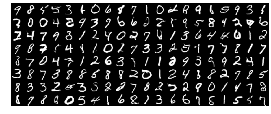
Figure 2: Random samples from DGAN trained on MNIST.

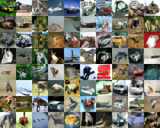
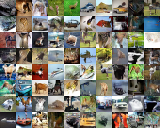
Figure 3: Random samples from DGAN trained on CIFAR10.

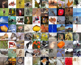
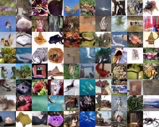
Figure 4: Random samples from DGAN trained on CIFAR100.

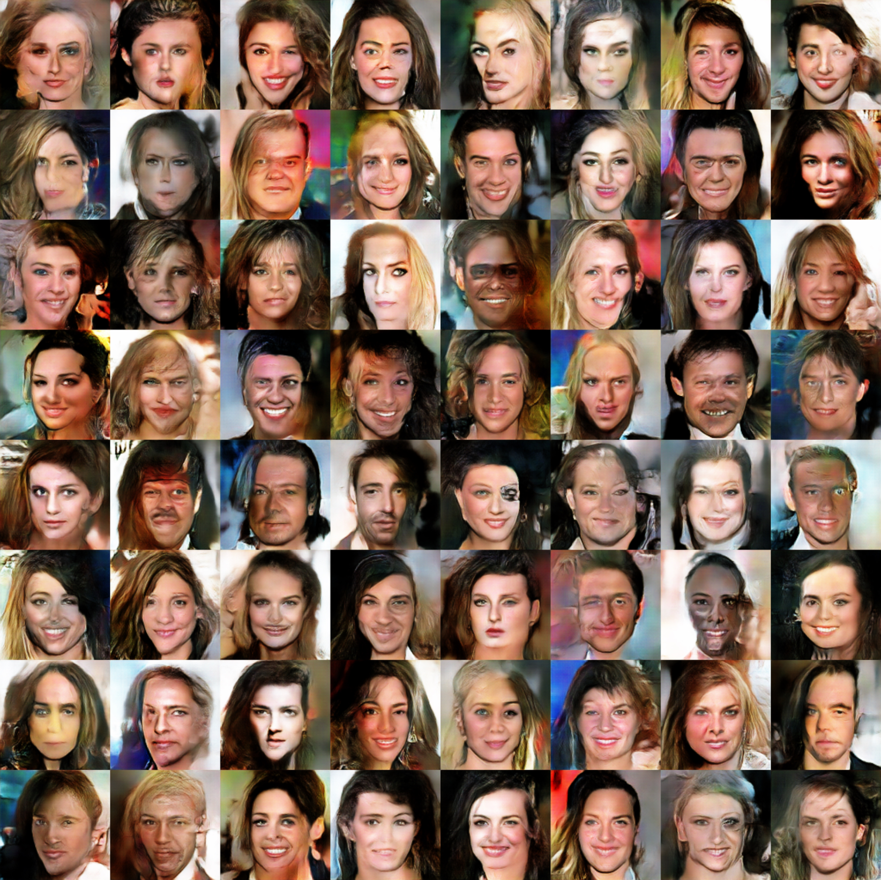
Figure 5: Random samples from DGAN trained on CelebA at resolution $128\times 128$.

To enforce the Lipschitz assumption of our Theorems, either weight clipping (Arjovsky et al., 2017),

Table 1: Inception Score (IS) and Fréchet Inception Distance (FID) for various datasets.

Dataset	IS	FID (train)	FID (test)
CIFAR10	7.02	26.7	30.7
CIFAR100	7.31	28.9	33.3
CelebA	2.15	59.2	-

gradient penalization (Gulrajani et al., 2017), spectral normalization (Miyato et al., 2018), or some combination can be used. We found gradient penalization useful for its stabilizing effect on training, and obtained the best performance with this and weight clipping. Table 1 lists Inception score (IS) and Fréchet Inception distance (FID) on various datasets. All results are the best of five trials. While our scores are not state-of-the-art (Brock et al., 2019), they are close to those achieved by similar unconditional DCGANs (Miyato et al., 2018; Lucic et al., 2018). Figures 2-5 show samples from a trained DGAN that are not cherry-picked.

4.2 EDGAN

Toy example

We first considered the toy datasets described in section 4.1 of AdaGAN (Tolstikhin et al., 2017), where we can explicitly compare various GANs with well-defined, likelihood-based performance metrics. The true data distribution is a mixture of 9 isotropic Gaussian components on $\mathcal{X}=\mathbb{R}^{2}$, with their centers uniformly distributed on a circle. We used the AdaGAN algorithm to sequentially generate 10 GANs, and compared various ensembles of these 10 networks: GAN₁ generated by the baseline GAN algorithm; Ada₅ and Ada₁₀, generated by AdaGAN with the first 5 or 10 GANs, respectively; EDGAN₅ and EDGAN₁₀, the ensembles of the first 5 or 10 GANs by EDGAN, respectively.

The EDGAN algorithm ran with squared loss and linear mappings. To measure the performance, we computed the likelihood of the generated data under the true distribution $L(S_{\theta})$, and the likelihood of the true data under the generated distribution $L(S_{r})$. We used kernel density estimation with cross-validated bandwidth to approximate the density of both $\mathbb{P}_{\theta}$ and $\mathbb{P}_{r}$, as in Tolstikhin et al. (2017). We provide part of the ensembles here and present the full results in Appendix C. Table 6 compares the two likelihood-based metrics averaged over 10 repetitions, with standard deviation in parentheses. We can see that for both metrics, ensembles of networks by EDGAN outperformed AdaGAN using the same number of base networks. Figure 6 shows the true distribution (in red) and the generated distribution (in blue). The single GAN model (Figure 6(a)) does not work well. As AdaGAN gradually mixes in more networks, the generated distribution is getting closer to the true distribution (Figure 6(b)). By explicitly learning the mixture weights using discrepancy, EDGAN₁₀ (Figure 6(c)) further improves over Ada₁₀, such that the span of the generated distribution is reduced, and the generated distribution now closely concentrates around the true one.

Table 2: Likelihood-based metrics of various ensembles of 10 GANs.

	$L(S_{r})$	$L(S_{\theta})$
GAN1	-12.39 ($\pm$ 2.12)	-796.05 ($\pm$ 12.48)
Ada10	-4.33 ($\pm$ 0.30)	-266.60 ($\pm$ 24.91)
EDGAN10	-3.99 ($\pm$ 0.20)	-148.97 ($\pm$ 14.13)

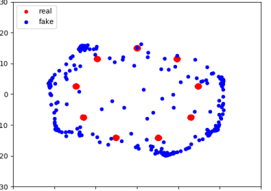
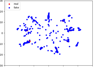
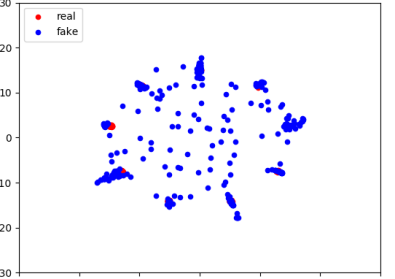
(a)	(b)	(c)

Figure 6: The true (red) and the generated (blue) distributions using (a) GAN₁; (b) Ada₁₀; (c) EDGAN₁₀.

CIFAR10

We used five pre-trained generators from Lucic et al. (2018) (all are publicly available on TF-Hub) as base learners in the ensemble. The models were trained with different hyperparameters and had different levels of performance. We then took 50k samples from each generator and the training split of CIFAR10, and embedded these images using a pre-trained classifier. We used several embeddings: InceptionV3’s logits layer (Szegedy et al., 2016), InceptionV3’s pooling layer (Szegedy et al., 2016), MobileNet (Sandler et al., 2018), PNASNet Liu et al. (2018a), NASNet (Zoph and Le, 2017), and AmoebaNet (Real et al., 2019). All of these models are also available on TF-Hub. For each embedding, we trained an ensemble and evaluated its discrepancy on the test set of CIFAR10 and 10k independent samples from each generator. We report these results in Table 3. In all cases EDGAN performs as well or better than the best individual generator or a uniform average of the generators. This also shows that discrepancy generalizes well from the training to the testing data. Interestingly, depending on which embedding is used for the ensemble, drastically different mixture weights are optimal, which demonstrates the importance of the hypothesis class for discrepancy. We list the learned ensemble weights in Table 5 in Appendix C.

Table 3: Each row uses a different embedding to calculate the discrepancy between the generated images and the CIFAR10 test set.

	GAN1	GAN2	GAN3	GAN4	GAN5	Best GAN	Average	EDGAN
InceptionLogits	285.09	259.61	259.64	271.21	272.23	259.61	259.12	255.3
InceptionPool	70.52	64.37	69.48	69.69	68.7	64.37	66.08	63.98
MobileNet	109.09	90.47	88.01	90.9	93.08	88.01	85.71	81.83
PNASNet	35.18	36.42	34.94	34.38	36.52	34.38	34.66	33.97
NASNet	54.61	52.66	59.01	61.79	64.97	52.66	55.66	52.46
AmoebaNet	97.71	110.83	108.61	105.31	110.5	97.71	104.91	97.71

5 Conclusion

We advocated the use of discrepancy for defining GANs and proved a series of favorable properties for it, including continuity, under mild assumptions, the possibility of accurately estimating it from finite samples, and the generalization guarantees it benefits from. We also showed empirically that DGAN is competitive with other GANs, and that EDGAN, which we showed can be formulated as a convex optimization problem, outperforms existing GAN ensembles. For future work, one can use generative models with discrepancy in adaptation, as shown in Appendix D, where the goal is to learn a feature embedding for the target domain such that its distribution is close to the distribution of the embedded source domain. DGAN also has connections with standard Maximum Entropy models (Maxent) as discussed in Appendix E.

Acknowledgments

This work was partly supported by NSF CCF-1535987, NSF IIS-1618662, and a Google Research Award. We thank Judy Hoffman for helpful pointers to the literature.

Appendix A GAN and WGAN

In this appendix section, we briefly introduce and discuss two instances of the distance metric $d$, which lead to two widely-used GANs: the original GAN [Goodfellow et al., 2014], and the WGAN [Arjovsky et al., 2017]. Note that in practice, often the value of $d(\mathbb{P},\mathbb{Q})$ is not directly computable, and its variational form is used instead.

A.1 GAN: Jensen-Shannon divergence

Goodfellow et al. [2014] introduced the first GAN framework using the Jensen-Shannon divergence:

$$d(\mathbb{P}_{r},\mathbb{P}_{\theta})\coloneqq\text{JS}(\mathbb{P}_{r},\mathbb{P}_{\theta})=\big{(}\,\text{KL}(\mathbb{P}_{r}\parallel\mathbb{P}_{m})+\,\text{KL}(\mathbb{P}_{\theta}\parallel\mathbb{P}_{m})\,\big{)}/2,$$

where $\mathbb{P}_{m}=(\mathbb{P}_{r}+\mathbb{P}_{\theta})/2$. The Jensen-Shannon divergence admits the following equivalent form:

$$\text{JS}(\mathbb{P}_{r},\mathbb{P}_{\theta})=\sup_{f\colon\mathcal{X}\to[0,1]}\frac{1}{2}\,\Big{\{}\operatorname*{\mathbb{E}}_{x\sim\mathbb{P}_{r}}\big{[}\log f(x)\big{]}+\operatorname*{\mathbb{E}}_{x\sim\mathbb{P}_{\theta}}\big{[}\log(1-f(x))\big{]}+\log 4\Big{\}}.$$ (4)

GANs were originally motivated by expression (4), and its equivalence to the Jensen-Shannon divergence was shown later on. Think of $f$ in equation (4) as a “discriminator” trying to tell apart real data from “fake” data generated by $g_{\theta}$ as follows: $f$ gives higher scores to samples which it thinks are real, and gives lower scores otherwise. Thus the maximization in (4) looks for the best discriminator $f$. On the other hand, the generator $g_{\theta}$ tries to fool the discriminator $f$, such that $f$ cannot tell the difference between real and fake samples. Thus minimizing $\text{JS}(\mathbb{P}_{r},\mathbb{P}_{\theta})$ over $\theta$ looks for the best generator $g_{\theta}$. Dropping the constants in (4) and parametrizing the discriminator $f$ with a family of neural networks $\{f_{w}\colon\mathcal{X}\to[0,1],w\in W\}$, the original algorithm of training GAN Goodfellow et al. [2014] considers the following min-max optimization problem:

$$\min_{\theta\in\Theta}\max_{w\in W}\Big{\{}\operatorname*{\mathbb{E}}_{x\sim\mathbb{P}_{r}}\big{[}\log f_{w}(x)\big{]}+\operatorname*{\mathbb{E}}_{x\sim\mathbb{P}_{\theta}}\big{[}\log(1-f_{w}(x))\big{]}\Big{\}}.$$ (5)

The generator and the discriminator $(g_{\theta},f_{w})$ are trained via stochastic gradient descent/ascent on objective (5) with respect to $\theta$ and $w$ iteratively, using the empirical distributions $\widehat{\mathbb{P}}_{r}$ and $\widehat{\mathbb{P}}_{\theta}$ induced by the batch of samples at each step.

Remark 1.

When minimizing $\theta$, one can drop the first term in (5) since it does not depend on $\theta$. Thus, for a fixed $w$, the minimizing step of $\theta$ is equivalent to $\min_{\theta}\operatorname*{\mathbb{E}}_{x\sim\mathbb{P}_{\theta}}\big{[}\log(1-f_{w}(x))\big{]}$. Goodfellow et al. [2014] suggested using maximization instead of minimization to speed up training for $\theta$. That is, the training of GAN iterates between

$$\max_{w\in W} \,\Big{\{}\operatorname*{\mathbb{E}}_{x\sim\mathbb{P}_{r}}\big{[}\log f_{w}(x)\big{]}+\operatorname*{\mathbb{E}}_{x\sim\mathbb{P}_{\theta}}\big{[}\log(1-f_{w}(x))\big{]}\Big{\}},$$

$$\max_{\theta\in\Theta} \,\Big{\{}\operatorname*{\mathbb{E}}_{x\sim\mathbb{P}_{\theta}}\big{[}\log f_{w}(x)\big{]}\Big{\}}.$$

A.2 WGAN: Wasserstein Distance

Instead of minimizing $\text{JS}(\mathbb{P}_{r},\mathbb{P}_{\theta})$, Arjovsky et al. [2017] proposed to use the Wasserstein distance:

$$d(\mathbb{P}_{r},\mathbb{P}_{\theta})\coloneqq W(\mathbb{P}_{r},\mathbb{P}_{\theta})=\inf_{\gamma\in\Pi(\mathbb{P}_{r},\mathbb{P}_{\theta})}\Big{\{}\operatorname*{\mathbb{E}}_{(x,y)\sim\gamma}\left\|x-y\right\|\Big{\}},$$

where $\Pi(\mathbb{P}_{r},\mathbb{P}_{\theta})=\{\gamma(x,y)\colon\int_{y}\gamma(x,y)dy=\mathbb{P}_{r}(x),\int_{x}\gamma(x,y)dx=\mathbb{P}_{\theta}(y)\}$ denotes the set of joint distributions whose marginals are $\mathbb{P}_{r}$ and $\mathbb{P}_{\theta}$, respectively. By the Kantorovich-Rubinstein duality [Villani, 2008], Wasserstein distance can also be written as

$$W(\mathbb{P}_{r},\mathbb{P}_{\theta})=\sup_{\left\|f\right\|_{L}\leq 1}\Big{\{}\operatorname*{\mathbb{E}}_{x\sim\mathbb{P}_{r}}\big{[}f(x)\big{]}-\operatorname*{\mathbb{E}}_{x\sim\mathbb{P}_{\theta}}\big{[}f(x)\big{]}\Big{\}},$$ (6)

where the supremum is taken over all $1$-Lipschitz functions with respect to the metric $\left\|\cdot\right\|$ that defines $W(\mathbb{P}_{r},\mathbb{P}_{\theta})$. Again, we can view $f$ as the discriminator, which aims to maximizes the difference between its expected values on the real data and that on the fake data. In practice, Arjovsky et al. [2017] set $f$ to be a neural networks whose parameters $w$ are limited within a compact set $W$, thus $\{f_{w}\colon w\in W\}$ is a set of $K$-Lipschitz functions for some constant $K$. Thus, the WGAN (Wasserstein GAN) considered the following min-max optimization problem:

$$\min_{\theta\in\Theta}\max_{w\in W}\Big{\{}\operatorname*{\mathbb{E}}_{x\sim\mathbb{P}_{r}}\big{[}f_{w}(x)\big{]}-\operatorname*{\mathbb{E}}_{x\sim\mathbb{P}_{\theta}}\big{[}f_{w}(x)\big{]}\Big{\}}.$$ (7)

The training procedure of WGANs is similar to that of GANs [Goodfellow et al., 2014], where one optimizes objective (7) using mini-batches with respect to $\theta$ and $w$ iteratively.

Arjovsky et al. [2017] showed that the JS divergence of GAN is potentially not continuous with respect to generator’s parameter $\theta$. On the other hand, under mild conditions, $W(\mathbb{P}_{r},\mathbb{P}_{\theta})$ is continuous everywhere and differentiable almost everywhere with respect to $\theta$, making it easier to train WGAN.

When training WGAN with (7), one need to clip the weights $w$ to ensure that $w\in W$. More recently, Gulrajani et al. [2017] found that weight clipping can lead to undesired behavior, such as capacity underuse, and exploding or vanishing gradients. In view of this, they proposed to add a gradient penalty to the objective of WGAN, as an alternative to weight clipping:

$$\min_{\theta\in\Theta}\max_{w}\Big{\{}\operatorname*{\mathbb{E}}_{x\sim\mathbb{P}_{r}}\big{[}f_{w}(x)\big{]}-\operatorname*{\mathbb{E}}_{x\sim\mathbb{P}_{\theta}}\big{[}f_{w}(x)\big{]}+\lambda\operatorname*{\mathbb{E}}_{x\sim\mathbb{P}_{l}}\big{[}\left(\left\|\nabla_{x}f_{w}\left(x\right)\right\|_{2}-1\right)^{2}\big{]}\Big{\}},$$

where $\mathbb{P}_{l}$ indicates the uniform distribution along straight lines between pairs of points in $S_{r}$ and $S_{\theta}$. The construction of $\mathbb{P}_{l}$ is motivated by the optimality conditions.

WGAN is closely related to DGAN. The definitions of Wasserstein distance (6) and discrepancy (1) are syntactically the same, except that the former takes supremum over all 1-Lipschitz functions, while the latter takes supremum over $\ell_{\mathcal{H}}=\big{\{}\ell\big{(}h(x),h^{\prime}(x)\big{)}\colon h,h^{\prime}\in\mathcal{H}\big{\}}$, a set that depends on the loss and hypothesis set. Thus, Wasserstein distance can be viewed as discrepancy without the hypothesis set and the loss function, which is one reason it cannot benefit from theoretical guarantees.

Appendix B Proofs

Theorem 1.

Assume the true labeling function $f\colon\mathcal{X}\to\mathcal{Y}$ is contained in the hypothesis set $\mathcal{H}$. Then, for any hypothesis $h\in\mathcal{H}$,

$$\operatorname*{\mathbb{E}}_{x\sim\mathbb{P}_{r}}[\ell(h,f)]\leq\operatorname*{\mathbb{E}}_{x\sim\mathbb{P}_{\theta}}[\ell(h,f)]+\text{disc}_{\mathcal{H},\ell}(\mathbb{P}_{\theta},\mathbb{P}_{r}).$$

Proof.

By the definition of $\text{disc}_{\mathcal{H},\ell}$, for any $h\in\mathcal{H}$,

$$\operatorname*{\mathbb{E}}_{x\sim\mathbb{P}_{r}}[\ell(h,f)] \leq\operatorname*{\mathbb{E}}_{x\sim\mathbb{P}_{\theta}}[\ell(h,f)]+\Big{|}\operatorname*{\mathbb{E}}_{x\sim\mathbb{P}_{r}}[\ell(h,f)]-\operatorname*{\mathbb{E}}_{x\sim\mathbb{P}_{\theta}}[\ell(h,f)]\,\Big{|}$$

$$\leq\operatorname*{\mathbb{E}}_{x\sim\mathbb{P}_{\theta}}[\ell(h,f)]+\sup_{h,h^{\prime}\in\mathcal{H}}\Big{|}\operatorname*{\mathbb{E}}_{x\sim\mathbb{P}_{r}}[\ell(h,h^{\prime})]-\operatorname*{\mathbb{E}}_{x\sim\mathbb{P}_{\theta}}[\ell(h,h^{\prime})]\,\Big{|} f\in\mathcal{H}$$ (Since )

$$=\operatorname*{\mathbb{E}}_{x\sim\mathbb{P}_{\theta}}[\ell(h,f)]+\text{disc}_{\mathcal{H},\ell}(\mathbb{P}_{\theta},\mathbb{P}_{r}).$$

∎

Proposition 6.

Let $\mathcal{H}$ be a set of 1-Lipschitz functions. Then, $\ell_{\mathcal{H}}=\big{\{}\big{[}h(x)-h^{\prime}(x)\big{]}^{2}\colon h,h^{\prime}\in\mathcal{H}\big{\}}$ is a set of Lipschitz functions on $\{x\colon\|x\|\leq 1\}$ with Lipschitz constant equals $4$.

Proof.

By definition,

$$|f(x)-f(x^{\prime})| =\big{|}\big{[}h(x)-h^{\prime}(x)\big{]}^{2}-\big{[}h(x^{\prime})-h^{\prime}(x^{\prime})\big{]}^{2}\big{|}$$

$$\leq 2\big{|}|h(x)-h^{\prime}(x)|-|h(x^{\prime})-h^{\prime}(x^{\prime})|\big{|} \ell_{2}$$ ( loss is 2-Lipschitz)

$$\leq 2\big{|}h(x)-h^{\prime}(x)-h(x^{\prime})+h^{\prime}(x^{\prime})\big{|}$$ (Triangle inequality)

$$\leq 2\big{|}h(x)-h(x^{\prime})|+2\big{|}h^{\prime}(x)-h^{\prime}(x^{\prime})\big{|}$$ (Triangle inequality)

$$\leq 4\|x-x^{\prime}\|. h h^{\prime}$$ ( and are 1-Lipschitz)

∎

Theorem 2.

Assume that $\mathcal{H}=\{h\colon\mathcal{X}\to\mathcal{Y}\}$ is a family of $\mu$-Lipschitz functions, and the loss function $\ell$ is continuous and symmetric in its arguments, and bounded by $M$. Furthermore, $\ell$ admits the triangle inequality, or it can be written as $\ell(y,y^{\prime})=f(|y-y^{\prime}|)$ for some Lipschitz function $f$. Assume that $g_{\theta}\colon\mathcal{Z}\to\mathcal{X}$ is continuous in $\theta$. Then, $\text{disc}_{\mathcal{H},\ell}(\mathbb{P}_{r},\mathbb{P}_{\theta})$ is continuous in $\theta$.

Proof.

We first consider the case where $\ell$ admits triangle inequality. We will show that $\text{disc}_{\mathcal{H},\ell}(\mathbb{P}_{\theta},\mathbb{P}_{\theta^{\prime}})\to 0$ as $\theta\to\theta^{\prime}$. By definition of $\mathbb{P}_{\theta}$ and $\text{disc}_{\mathcal{H},\ell}$,

$$\text{disc}_{\mathcal{H},\ell}(\mathbb{P}_{\theta},\mathbb{P}_{\theta^{\prime}}) =\sup_{h,h^{\prime}\in\mathcal{H}}\bigg{|}\operatorname*{\mathbb{E}}_{z\sim\mathbb{P}_{z}}\Big{[}\ell\Big{(}h\big{(}g_{\theta}(z)\big{)},h^{\prime}\big{(}g_{\theta}(z)\big{)}\Big{)}-\ell\Big{(}h\big{(}g_{\theta^{\prime}}(z)\big{)},h^{\prime}\big{(}g_{\theta^{\prime}}(z)\big{)}\Big{)}\Big{]}\bigg{|}$$

$$\leq\sup_{h,h^{\prime}\in\mathcal{H}}\operatorname*{\mathbb{E}}_{z\sim\mathbb{P}_{z}}\bigg{|}\ell\Big{(}h\big{(}g_{\theta}(z)\big{)},h^{\prime}\big{(}g_{\theta}(z)\big{)}\Big{)}-\ell\Big{(}h\big{(}g_{\theta^{\prime}}(z)\big{)},h^{\prime}\big{(}g_{\theta^{\prime}}(z)\big{)}\Big{)}\bigg{|}$$

$$\leq\sup_{h,h^{\prime}\in\mathcal{H}}\operatorname*{\mathbb{E}}_{z\sim\mathbb{P}_{z}}\bigg{[}\ell\Big{(}h\big{(}g_{\theta}(z)\big{)},h\big{(}g_{\theta^{\prime}}(z)\big{)}\Big{)}+\ell\Big{(}h^{\prime}\big{(}g_{\theta}(z)\big{)},h^{\prime}\big{(}g_{\theta^{\prime}}(z)\big{)}\Big{)}\bigg{]},$$

where we used the triangle inequality and symmetry of $\ell$, such that $\forall a,b,c,d\in\mathcal{Y}$,

$$|\ell(a,b)-\ell(c,d)| \leq\ell(a,c)+\ell(b,d).$$

Thus,

$$\text{disc}_{\mathcal{H},\ell}(\mathbb{P}_{\theta},\mathbb{P}_{\theta^{\prime}})\leq\sup_{h\in\mathcal{H}}2\operatorname*{\mathbb{E}}_{z\sim\mathbb{P}_{z}}\bigg{[}\ell\Big{(}h\big{(}g_{\theta}(z)\big{)},h\big{(}g_{\theta^{\prime}}(z)\big{)}\Big{)}\bigg{]}\leq 2\operatorname*{\mathbb{E}}_{z\sim\mathbb{P}_{z}}\bigg{[}\sup_{h\in\mathcal{H}}\ell\Big{(}h\big{(}g_{\theta}(z)\big{)},h\big{(}g_{\theta^{\prime}}(z)\big{)}\Big{)}\bigg{]}.$$

Since $\forall h\in\mathcal{H}$ is $L$-Lipschitz, for any $x_{0}\in\mathcal{X}$,

$$\lim_{x\to x_{0}}\ell\Big{(}h(x),h(x_{0})\Big{)}=0$$

converges uniformly over $h\in\mathcal{H}$. Furthermore, $g_{\theta}$ is continuous in $\theta$, it follows that for any fixed $z\in\mathcal{Z}$,

$$\lim_{\theta\to\theta^{\prime}}\sup_{h\in\mathcal{H}}\ell\Big{(}h\big{(}g_{\theta}(z)\big{)},h\big{(}g_{\theta^{\prime}}(z)\big{)}\Big{)}=0,$$

thus converges point-wise as functions of $z$. Since $\ell\leq M$ is bounded, by bounded convergence theorem, we have

$$\lim_{\theta\to\theta^{\prime}}\text{disc}_{\mathcal{H},\ell}(\mathbb{P}_{\theta},\mathbb{P}_{\theta^{\prime}})\leq 2\lim_{\theta\to\theta^{\prime}}\operatorname*{\mathbb{E}}_{z\sim\mathbb{P}_{z}}\bigg{[}\sup_{h\in\mathcal{H}}\ell\Big{(}h\big{(}g_{\theta}(z)\big{)},h\big{(}g_{\theta^{\prime}}(z)\big{)}\Big{)}\bigg{]}=0.$$

Now we consider the case where $\ell(a,b)=f(|a-b|)$, and $f$ is a $q$-Lipschitz function: $|f(x)-f(x^{\prime})|\leq q|x-x^{\prime}|$. By definition,

$$\text{disc}_{\mathcal{H},\ell}(\mathbb{P}_{\theta},\mathbb{P}_{\theta^{\prime}}) =\sup_{h,h^{\prime}\in\mathcal{H}}\bigg{|}\operatorname*{\mathbb{E}}_{z\sim\mathbb{P}_{z}}\Big{[}\ell\Big{(}h\big{(}g_{\theta}(z)\big{)},h^{\prime}\big{(}g_{\theta}(z)\big{)}\Big{)}-\ell\Big{(}h\big{(}g_{\theta^{\prime}}(z)\big{)},h^{\prime}\big{(}g_{\theta^{\prime}}(z)\big{)}\Big{)}\Big{]}\bigg{|}$$

$$\leq\sup_{h,h^{\prime}\in\mathcal{H}}\operatorname*{\mathbb{E}}_{z\sim\mathbb{P}_{z}}\bigg{|}\ell\Big{(}h\big{(}g_{\theta}(z)\big{)},h^{\prime}\big{(}g_{\theta}(z)\big{)}\Big{)}-\ell\Big{(}h\big{(}g_{\theta^{\prime}}(z)\big{)},h^{\prime}\big{(}g_{\theta^{\prime}}(z)\big{)}\Big{)}\bigg{|}$$

$$=\sup_{h,h^{\prime}\in\mathcal{H}}\operatorname*{\mathbb{E}}_{z\sim\mathbb{P}_{z}}\bigg{|}f\Big{(}\big{|}h\big{(}g_{\theta}(z)\big{)}-h^{\prime}\big{(}g_{\theta}(z)\big{)}\big{|}\Big{)}-f\Big{(}\big{|}h\big{(}g_{\theta^{\prime}}(z)\big{)}-h^{\prime}\big{(}g_{\theta^{\prime}}(z)\big{)}\big{|}\Big{)}\bigg{|}$$

$$\leq q\,\sup_{h,h^{\prime}\in\mathcal{H}}\operatorname*{\mathbb{E}}_{z\sim\mathbb{P}_{z}}\bigg{|}\Big{|}h\big{(}g_{\theta}(z)\big{)}-h^{\prime}\big{(}g_{\theta}(z)\big{)}\Big{|}-\Big{|}h\big{(}g_{\theta^{\prime}}(z)\big{)}-h^{\prime}\big{(}g_{\theta^{\prime}}(z)\big{)}\Big{|}\bigg{|}$$

$$\leq q\,\sup_{h,h^{\prime}\in\mathcal{H}}\operatorname*{\mathbb{E}}_{z\sim\mathbb{P}_{z}}\bigg{|}h\big{(}g_{\theta}(z)\big{)}-h\big{(}g_{\theta^{\prime}}(z)\big{)}-h^{\prime}\big{(}g_{\theta}(z)\big{)}+h^{\prime}\big{(}g_{\theta^{\prime}}(z)\big{)}\bigg{|}$$

$$\leq q\,\sup_{h,h^{\prime}\in\mathcal{H}}\operatorname*{\mathbb{E}}_{z\sim\mathbb{P}_{z}}\bigg{[}\Big{|}h\big{(}g_{\theta}(z)\big{)}-h\big{(}g_{\theta^{\prime}}(z)\big{)}\Big{|}+\Big{|}h^{\prime}\big{(}g_{\theta}(z)\big{)}-h^{\prime}\big{(}g_{\theta^{\prime}}(z)\big{)}\Big{|}\bigg{]}$$

$$=2q\,\sup_{h\in\mathcal{H}}\operatorname*{\mathbb{E}}_{z\sim\mathbb{P}_{z}}\Big{|}h\big{(}g_{\theta}(z)\big{)}-h\big{(}g_{\theta^{\prime}}(z)\big{)}\Big{|}$$

$$\leq 2q\,\operatorname*{\mathbb{E}}_{z\sim\mathbb{P}_{z}}\sup_{h\in\mathcal{H}}\Big{|}h\big{(}g_{\theta}(z)\big{)}-h\big{(}g_{\theta^{\prime}}(z)\big{)}\Big{|}.$$

Then, by the same argument above,

$$\lim_{\theta\to\theta^{\prime}}\text{disc}_{\mathcal{H},\ell}(\mathbb{P}_{\theta},\mathbb{P}_{\theta^{\prime}})\leq 2q\lim_{\theta\to\theta^{\prime}}\operatorname*{\mathbb{E}}_{z\sim\mathbb{P}_{z}}\sup_{h\in\mathcal{H}}\Big{|}h\big{(}g_{\theta}(z)\big{)},h\big{(}g_{\theta^{\prime}}(z)\big{)}\Big{|}=0.$$

Finally, by the triangle inequality of $\text{disc}_{\mathcal{H},\ell}$, $\text{disc}_{\mathcal{H},\ell}(\mathbb{P}_{r},\mathbb{P}_{\theta})-\text{disc}_{\mathcal{H},\ell}(\mathbb{P}_{r},\mathbb{P}_{\theta^{\prime}})\leq\text{disc}_{\mathcal{H},\ell}(\mathbb{P}_{\theta},\mathbb{P}_{\theta^{\prime}})$, which completes the proof. ∎

Theorem 3.

Assume the loss is bounded, $\ell\leq M$. For any $\delta>0$, with probability at least $1-\delta$ over the drawn of $S_{r}$ and $S_{\theta}$,

$$\big{|}\text{disc}_{\mathcal{H},\ell}(\mathbb{P}_{r},\mathbb{P}_{\theta})-\text{disc}_{\mathcal{H},\ell}(\widehat{\mathbb{P}}_{r},\widehat{\mathbb{P}}_{\theta})\big{|}\leq\widehat{\mathfrak{R}}_{S_{r}}(\ell_{\mathcal{H}})+\widehat{\mathfrak{R}}_{S_{\theta}}(\ell_{\mathcal{H}})+3M\Big{(}\sqrt{\tfrac{\log(4/\delta)}{2m}}+\sqrt{\tfrac{\log(4/\delta)}{2n}}\,\Big{)}.$$

Furthermore, when the loss function $\ell(h,h^{\prime})$ is a $q$-Lipschitz function of $h-h^{\prime}$, we have

$$\big{|}\text{disc}_{\mathcal{H},\ell}(\mathbb{P}_{r},\mathbb{P}_{\theta})-\text{disc}_{\mathcal{H},\ell}(\widehat{\mathbb{P}}_{r},\widehat{\mathbb{P}}_{\theta})\big{|}\leq 4q\Big{(}\widehat{\mathfrak{R}}_{S_{r}}(\mathcal{H})+\widehat{\mathfrak{R}}_{S_{\theta}}(\mathcal{H})\Big{)}+3M\Big{(}\sqrt{\tfrac{\log(4/\delta)}{2m}}+\sqrt{\tfrac{\log(4/\delta)}{2n}}\Big{)}.$$

Proof.

By triangle inequality of $\text{disc}_{\mathcal{H},\ell}(\cdot,\cdot)$,

$$|\text{disc}_{\mathcal{H},\ell}(\mathbb{P}_{r},\mathbb{P}_{\theta})-\text{disc}_{\mathcal{H},\ell}(\widehat{\mathbb{P}}_{r},\widehat{\mathbb{P}}_{\theta})|\leq\text{disc}_{\mathcal{H},\ell}(\mathbb{P}_{r},\widehat{\mathbb{P}}_{r})+\text{disc}_{\mathcal{H},\ell}(\mathbb{P}_{\theta},\widehat{\mathbb{P}}_{\theta}).$$

We first apply concentration inequality to the scaled loss $\ell_{\mathcal{H}}/M$:

$$\operatorname*{\mathbb{E}}_{\mathbb{P}_{r}}\ell(h,h^{\prime})/M \leq\operatorname*{\mathbb{E}}_{\widehat{\mathbb{P}}_{r}}\ell(h,h^{\prime})/M+\widehat{\mathfrak{R}}_{S_{r}}(\ell_{\mathcal{H}}/M)+3\sqrt{\frac{\log(4/\delta)}{2m}},$$

$$\operatorname*{\mathbb{E}}_{\mathbb{P}_{\theta}}\ell(h,h^{\prime})/M \leq\operatorname*{\mathbb{E}}_{\widehat{\mathbb{P}}_{\theta}}\ell(h,h^{\prime})/M+\widehat{\mathfrak{R}}_{S_{\theta}}(\ell_{\mathcal{H}}/M).$$

For the empirical Radmacher complexity, we have $\widehat{\mathfrak{R}}_{c\mathcal{H}}=c\widehat{\mathfrak{R}}_{\mathcal{H}}$. Thus, we have

$$|\text{disc}_{\mathcal{H},\ell}(\mathbb{P}_{r},\mathbb{P}_{\theta})-\text{disc}_{\mathcal{H},\ell}(\widehat{\mathbb{P}}_{r},\widehat{\mathbb{P}}_{\theta})|$$

$$\leq\text{disc}_{\mathcal{H},\ell}(\mathbb{P}_{r},\widehat{\mathbb{P}}_{r})+\text{disc}_{\mathcal{H},\ell}(\mathbb{P}_{\theta},\widehat{\mathbb{P}}_{\theta})\leq\widehat{\mathfrak{R}}_{S_{r}}(\ell_{\mathcal{H}})+\widehat{\mathfrak{R}}_{S_{\theta}}(\ell_{\mathcal{H}})+3M\bigg{(}\sqrt{\frac{\log(4/\delta)}{2m}}+\sqrt{\frac{\log(4/\delta)}{2n}}\bigg{)}.$$

When the loss function $\ell(h,h^{\prime})$ is a $q$-Lipschitz function of the difference of its two arguments, i.e. $\ell(a,b)=f(a-b)$, and $f(\cdot)$ is a $q$-Lipschitz function, the mapping of $\mathcal{H}\ominus\mathcal{H}\to\ell_{\mathcal{H}}$ is $q$-Lipschitz, where $\mathcal{H}\ominus\mathcal{H}$ is defined as $\mathcal{H}\ominus\mathcal{H}=\{h-h^{\prime}\colon h,h^{\prime}\in\mathcal{H}\}$. By Talagrand’s contraction lemma, $\widehat{\mathfrak{R}}_{\ell_{\mathcal{H}}}\leq 2q\mathfrak{R}_{\mathcal{H}\ominus\mathcal{H}}$. Finally, by definition we have $\widehat{\mathfrak{R}}_{\mathcal{H}\ominus\mathcal{H}}\leq 2\widehat{\mathfrak{R}}_{\mathcal{H}}$. Putting everything together, when the loss function $\ell(h,h^{\prime})$ is a $q$-Lipschitz function of $h-h^{\prime}$,

$$|\text{disc}_{\mathcal{H},\ell}(\mathbb{P}_{r},\mathbb{P}_{\theta})-\text{disc}_{\mathcal{H},\ell}(\widehat{\mathbb{P}}_{r},\widehat{\mathbb{P}}_{\theta})|\leq 4q\Big{(}\widehat{\mathfrak{R}}_{S_{r}}(\mathcal{H})+\widehat{\mathfrak{R}}_{S_{\theta}}(\mathcal{H})\Big{)}+3M\bigg{(}\sqrt{\frac{\log(4/\delta)}{2m}}+\sqrt{\frac{\log(4/\delta)}{2n}}\bigg{)}.$$

∎

Theorem 5.

For any $\delta>0$, with probability at least $1-\delta$ over the draw of samples,

$$|\text{disc}_{\mathcal{H},\ell}(\mathbb{P}_{{\widehat{\boldsymbol{\alpha}}}},\mathbb{P}_{r})-\text{disc}_{\mathcal{H},\ell}(\mathbb{P}_{{\boldsymbol{\alpha}^{*}}},\mathbb{P}_{r})|\leq 2\Big{(}\widehat{\mathfrak{R}}_{S}(\ell_{\mathcal{H}})+3M\sqrt{{\log[4(p+1)/\delta]}/{2n}}\,\Big{)},$$

where $\widehat{\mathfrak{R}}_{S}(\ell_{\mathcal{H}})=\max\big{\{}\widehat{\mathfrak{R}}_{S_{1}}(\ell_{\mathcal{H}}),\ldots,\widehat{\mathfrak{R}}_{S_{p}}(\ell_{\mathcal{H}}),\widehat{\mathfrak{R}}_{S_{r}}(\ell_{\mathcal{H}})\big{\}}$. Furthermore, when the loss function $\ell(h,h^{\prime})$ is a $q$-Lipschitz function of $h-h^{\prime}$, the following holds with probability $1-\delta$:

$$|\text{disc}_{\mathcal{H},\ell}(\mathbb{P}_{{\widehat{\boldsymbol{\alpha}}}},\mathbb{P}_{r})-\text{disc}_{\mathcal{H},\ell}(\mathbb{P}_{{\boldsymbol{\alpha}^{*}}},\mathbb{P}_{r})|\leq 2\Big{(}4q\,\widehat{\mathfrak{R}}_{S}(\mathcal{H})+3M\sqrt{{\log[4(p+1)/\delta]}/{2n}}\,\Big{)},$$

where $\widehat{\mathfrak{R}}_{S}(\mathcal{H})=\max\big{\{}\widehat{\mathfrak{R}}_{S_{1}}({\mathcal{H}}),\ldots,\widehat{\mathfrak{R}}_{S_{p}}({\mathcal{H}}),\widehat{\mathfrak{R}}_{S_{r}}({\mathcal{H}})\big{\}}$.

Proof.

We first extend Theorem 3 to the case of GAN ensembles:

$$|\text{disc}_{\mathcal{H},\ell}({\mathbb{P}}_{\boldsymbol{\alpha}},\mathbb{P}_{r})-\text{disc}_{\mathcal{H},\ell}(\widehat{\mathbb{P}}_{\boldsymbol{\alpha}},\widehat{\mathbb{P}}_{r})|\leq\text{disc}_{\mathcal{H},\ell}({\mathbb{P}}_{\boldsymbol{\alpha}},\widehat{\mathbb{P}}_{\boldsymbol{\alpha}})+\text{disc}_{\mathcal{H},\ell}(\mathbb{P}_{r},\widehat{\mathbb{P}}_{r}).$$

For the first term,

$$\text{disc}_{\mathcal{H},\ell}({\mathbb{P}}_{\boldsymbol{\alpha}},\widehat{\mathbb{P}}_{\boldsymbol{\alpha}})$$

$$\leq\sup_{h,h^{\prime}\in\mathcal{H}}\Big{|}\sum_{k=1}^{p}\alpha_{k}\Big{\{}\operatorname*{\mathbb{E}}_{x\sim\mathbb{P}_{k}}\big{[}\ell\big{(}h(x),h^{\prime}(x)\big{)}\big{]}-\operatorname*{\mathbb{E}}_{x\sim\widehat{\mathbb{P}}_{k}}\big{[}\ell\big{(}h(x),h^{\prime}(x)\big{)}\big{]}\Big{\}}\Big{|}$$

$$\leq\sup_{h,h^{\prime}\in\mathcal{H}}\sum_{k=1}^{p}\alpha_{k}\Big{|}\operatorname*{\mathbb{E}}_{x\sim\mathbb{P}_{k}}\big{[}\ell\big{(}h(x),h^{\prime}(x)\big{)}\big{]}-\operatorname*{\mathbb{E}}_{x\sim\widehat{\mathbb{P}}_{k}}\big{[}\ell\big{(}h(x),h^{\prime}(x)\big{)}\big{]}\Big{|}$$

$$\leq\sum_{k=1}^{p}\alpha_{k}\sup_{h,h^{\prime}\in\mathcal{H}}\Big{|}\operatorname*{\mathbb{E}}_{x\sim\mathbb{P}_{k}}\big{[}\ell\big{(}h(x),h^{\prime}(x)\big{)}\big{]}-\operatorname*{\mathbb{E}}_{x\sim\widehat{\mathbb{P}}_{k}}\big{[}\ell\big{(}h(x),h^{\prime}(x)\big{)}\big{]}\Big{|}$$

$$=\sum_{k=1}^{p}\alpha_{k}\,\text{disc}_{\mathcal{H},\ell}(\mathbb{P}_{k},\widehat{\mathbb{P}}_{k}).$$

By concentration argument, with probability at least $1-\delta$ over the drawn of samples,

$$\text{disc}_{\mathcal{H},\ell}(\mathbb{P}_{r},\widehat{\mathbb{P}}_{r}) \leq\widehat{\mathfrak{R}}_{S_{r}}(\ell_{\mathcal{H}})+3M\sqrt{\frac{\log(4(p+1)/\delta)}{2n}},$$

$$\text{disc}_{\mathcal{H},\ell}(\mathbb{P}_{k},\widehat{\mathbb{P}}_{k}) \leq\widehat{\mathfrak{R}}_{S_{k}}(\ell_{\mathcal{H}})+3M\sqrt{\frac{\log(4(p+1)/\delta)}{2n}}.$$

Putting everything together, with probability at least $1-\delta$, for any $\alpha\in\Delta$,

$$|\text{disc}_{\mathcal{H},\ell}({\mathbb{P}}_{\boldsymbol{\alpha}},\mathbb{P}_{r})-\text{disc}_{\mathcal{H},\ell}(\widehat{\mathbb{P}}_{\boldsymbol{\alpha}},\widehat{\mathbb{P}}_{r})|$$

$$\leq\sum_{k=1}^{n}\alpha_{k}\,\text{disc}_{\mathcal{H},\ell}(\mathbb{P}_{k},\widehat{\mathbb{P}}_{k})+\text{disc}_{\mathcal{H},\ell}(\mathbb{P}_{r},\widehat{\mathbb{P}}_{r})$$

$$\leq\sum_{k=1}^{n}\alpha_{k}\,\bigg{[}\widehat{\mathfrak{R}}_{S_{k}}(\ell_{\mathcal{H}})+3M\sqrt{\frac{\log(4(p+1)/\delta)}{2n}}\bigg{]}+\widehat{\mathfrak{R}}_{S_{r}}(\ell_{\mathcal{H}})+3M\sqrt{\frac{\log(4(p+1)/\delta)}{2n}}$$

$$\leq\widehat{\mathfrak{R}}_{S}+3M\sqrt{\frac{\log(4(p+1)/\delta)}{2n}}.$$ (8)

By definition,

$$\text{disc}_{\mathcal{H},\ell}(\mathbb{P}_{{\boldsymbol{\alpha}^{*}}},\mathbb{P}_{r})-\text{disc}_{\mathcal{H},\ell}(\mathbb{P}_{{\widehat{\boldsymbol{\alpha}}}},\mathbb{P}_{r})$$

$$\leq\text{disc}_{\mathcal{H},\ell}(\mathbb{P}_{{\boldsymbol{\alpha}^{*}}},\mathbb{P}_{r})-\text{disc}_{\mathcal{H},\ell}(\widehat{\mathbb{P}}_{{\widehat{\boldsymbol{\alpha}}}},\widehat{\mathbb{P}}_{r})+|\text{disc}_{\mathcal{H},\ell}(\widehat{\mathbb{P}}_{{\widehat{\boldsymbol{\alpha}}}},\widehat{\mathbb{P}}_{r})-\text{disc}_{\mathcal{H},\ell}(\mathbb{P}_{{\widehat{\boldsymbol{\alpha}}}},\mathbb{P}_{r})|$$

$$\leq\text{disc}_{\mathcal{H},\ell}(\mathbb{P}_{{\widehat{\boldsymbol{\alpha}}}},\mathbb{P}_{r})-\text{disc}_{\mathcal{H},\ell}(\widehat{\mathbb{P}}_{{\widehat{\boldsymbol{\alpha}}}},\widehat{\mathbb{P}}_{r})+|\text{disc}_{\mathcal{H},\ell}(\widehat{\mathbb{P}}_{{\widehat{\boldsymbol{\alpha}}}},\widehat{\mathbb{P}}_{r})-\text{disc}_{\mathcal{H},\ell}(\mathbb{P}_{{\widehat{\boldsymbol{\alpha}}}},\mathbb{P}_{r})|$$

$$\leq 2|\text{disc}_{\mathcal{H},\ell}(\widehat{\mathbb{P}}_{{\widehat{\boldsymbol{\alpha}}}},\widehat{\mathbb{P}}_{r})-\text{disc}_{\mathcal{H},\ell}(\mathbb{P}_{{\widehat{\boldsymbol{\alpha}}}},\mathbb{P}_{r})|$$

Similarly,

$$\text{disc}_{\mathcal{H},\ell}(\mathbb{P}_{{\widehat{\boldsymbol{\alpha}}}},\mathbb{P}_{r})-\text{disc}_{\mathcal{H},\ell}(\mathbb{P}_{{\boldsymbol{\alpha}^{*}}},\mathbb{P}_{r})$$

$$\leq \text{disc}_{\mathcal{H},\ell}(\mathbb{P}_{{\widehat{\boldsymbol{\alpha}}}},\mathbb{P}_{r})-\text{disc}_{\mathcal{H},\ell}(\widehat{\mathbb{P}}_{{\boldsymbol{\alpha}^{*}}},\widehat{\mathbb{P}}_{r})+|\text{disc}_{\mathcal{H},\ell}(\widehat{\mathbb{P}}_{{\boldsymbol{\alpha}^{*}}},\widehat{\mathbb{P}}_{r})-\text{disc}_{\mathcal{H},\ell}(\mathbb{P}_{{\boldsymbol{\alpha}^{*}}},\mathbb{P}_{r})|$$

$$\leq \text{disc}_{\mathcal{H},\ell}(\mathbb{P}_{{\widehat{\boldsymbol{\alpha}}}},\mathbb{P}_{r})-\text{disc}_{\mathcal{H},\ell}(\widehat{\mathbb{P}}_{{\widehat{\boldsymbol{\alpha}}}},\widehat{\mathbb{P}}_{r})+|\text{disc}_{\mathcal{H},\ell}(\widehat{\mathbb{P}}_{{\boldsymbol{\alpha}^{*}}},\widehat{\mathbb{P}}_{r})-\text{disc}_{\mathcal{H},\ell}(\mathbb{P}_{{\boldsymbol{\alpha}^{*}}},\mathbb{P}_{r})|$$

$$\leq |\text{disc}_{\mathcal{H},\ell}(\mathbb{P}_{{\widehat{\boldsymbol{\alpha}}}},\mathbb{P}_{r})-\text{disc}_{\mathcal{H},\ell}(\widehat{\mathbb{P}}_{{\widehat{\boldsymbol{\alpha}}}},\widehat{\mathbb{P}}_{r})|+|\text{disc}_{\mathcal{H},\ell}(\widehat{\mathbb{P}}_{{\boldsymbol{\alpha}^{*}}},\widehat{\mathbb{P}}_{r})-\text{disc}_{\mathcal{H},\ell}(\mathbb{P}_{{\boldsymbol{\alpha}^{*}}},\mathbb{P}_{r})|.$$

Thus, apply inequality (B) to $\widehat{\boldsymbol{\alpha}}$ and $\boldsymbol{\alpha}^{*}$, we have

$$|\text{disc}_{\mathcal{H},\ell}(\mathbb{P}_{{\widehat{\boldsymbol{\alpha}}}},\mathbb{P}_{r})-\text{disc}_{\mathcal{H},\ell}(\mathbb{P}_{{\boldsymbol{\alpha}^{*}}},\mathbb{P}_{r})|\leq 2\Big{(}\widehat{\mathfrak{R}}_{S}+3M\sqrt{\frac{\log(4(p+1)/\delta)}{2n}}\Big{)}.$$

∎

Proposition 4.

When $\ell$ is the squared loss and $\mathcal{H}$ the family of linear functions with norm bounded by $1$, $\text{disc}_{\mathcal{H},\ell}(\widehat{\mathbb{P}}_{r},\widehat{\mathbb{P}}_{\theta})=2\left\|\frac{1}{n}X_{\theta}^{T}X_{\theta}-\frac{1}{m}X_{r}^{T}X_{r}\right\|_{2}$, where $\|\cdot\|_{2}$ denotes the spectral norm.

Proof.

$$\text{disc}_{\mathcal{H},\ell}(\widehat{\mathbb{P}}_{r},\widehat{\mathbb{P}}_{\theta})= \sup_{\begin{subarray}{c}\parallel w\parallel_{2}\leq 1\\ \parallel w^{\prime}\parallel_{2}\leq 1\end{subarray}}\Big{|}\operatorname*{\mathbb{E}}_{x\sim\widehat{\mathbb{P}}_{r}}\big{[}\ell_{2}\big{(}w^{T}x,w^{\prime T}x\big{)}-\operatorname*{\mathbb{E}}_{x\sim\widehat{\mathbb{P}}_{\theta}}\big{[}\ell_{2}\big{(}w^{T}x,w^{\prime T}x\big{)}\Big{|}$$

$$= \sup_{\begin{subarray}{c}\parallel w\parallel_{2}\leq 1\\ \parallel w^{\prime}\parallel_{2}\leq 1\end{subarray}}\Big{|}\frac{1}{n}(X_{\theta}w-X_{\theta}w^{\prime})^{T}(X_{\theta}w-X_{\theta}w^{\prime})-\frac{1}{m}(X_{r}w-X_{r}w^{\prime})^{T}(X_{r}w-X_{r}w^{\prime})\Big{|}$$

$$= \sup_{\parallel u\parallel_{2}\leq 2}\Big{|}\frac{1}{n}u^{T}X_{\theta}^{T}X_{\theta}u-\frac{1}{m}u^{T}X_{r}^{T}X_{r}u\Big{|} u=w-w^{\prime}$$ (Let )

$$= 2\sup_{\parallel u\parallel_{2}\leq 1}\Big{|}u^{T}\Big{(}\frac{1}{n}X_{\theta}^{T}X_{\theta}-\frac{1}{m}X_{r}^{T}X_{r}\Big{)}u\Big{|}$$

$$= 2\left\|\frac{1}{n}X_{\theta}^{T}X_{\theta}-\frac{1}{m}X_{r}^{T}X_{r}\right\|_{2}.$$

∎

Appendix C More Experiments

C.1 EDGAN: Toy datasets

In this section, we provide more results on mixing the 10 GANs generated by AdaGAN. Recall that we are comparing the following methods:

• The baseline GAN algorithm, namely GAN₁.

• The AdaGAN algorithm, ensembles of the first 5 GANs, namely Ada₅.

• The AdaGAN algorithm, ensembles of the first 10 GANs, namely Ada₁₀.

• The EDGAN algorithm, ensembles of the first 5 GANs, namely EDGAN₅.

• The EDGAN algorithm, ensembles of the first 10 GANs, namely EDGAN₁₀.

We considered two ways of computing average sample log-likelihood and used them as performance metrics: the likelihood of the generated data under the true distribution $L(S_{\theta})$, and the likelihood of the true data under the generated distribution $L(S_{r})$. To be more concrete,

$$L(S_{\theta})=L_{\mathbb{P}_{r}}(S_{\theta})=\frac{1}{N}\sum_{x_{i}\in S_{\theta}}\log\big{(}\mathbb{P}_{r}(x_{i})\big{)},\quad L(S_{r})=L_{\mathbb{P}_{\theta}}(S_{r})=\frac{1}{N}\sum_{x_{i}\in S_{r}}\log\big{(}\mathbb{P}_{\theta}(x_{i})\big{)}.$$

We used kernel density estimation with cross-validated bandwidth to approximate the density of both $\mathbb{P}_{\theta}$ and $\mathbb{P}_{r}$.

Figure 7 displayed the true distribution (in red) and the generated distribution under various ensembles of GANs. EDGAN₅ and EDGAN₁₀ improve the generated distribution over Ada₅ and Ada₁₀, respectively.

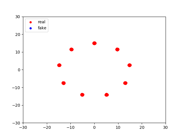
(a) $\mathbb{P}_{r}$

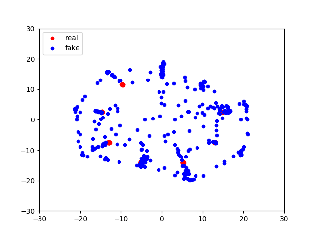
(b) Ada₅

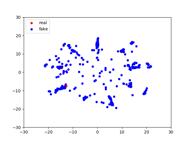
(c) Ada₁₀

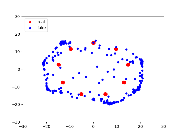
(d) GAN₁

(e) EDGAN₅

(f) EDGAN₁₀

Figure 7: The true (red) and the generated (blue) distributions, using various ensembles of 10 GANs.

Table 4 showed the average log-likelihoods over 10 repetitions, with standard deviations in parentheses, where a higher log-likelihood indicates better performance. We can see that for both metrics, networks ensembles EDGAN₅ and EDGAN₁₀ by EDGAN outperformed AdaGAN with the same number of base networks.

Table 4: Likelihood-based metrics of various ensembles of 10 GANs.

	$L(S_{r})$	$L(S_{\theta})$
GAN1	-12.39 ($\pm$ 2.12)	-796.05 ($\pm$ 12.48)
Ada5	-5.02 ($\pm$ 0.11)	-296.45 ($\pm$ 15.24)
Ada10	-4.33 ($\pm$ 0.30)	-266.60 ($\pm$ 24.91)
EDGAN5	-4.85 ($\pm$ 0.16)	-172.52 ($\pm$ 17.56)
EDGAN10	-3.99 ($\pm$ 0.20)	-148.97 ($\pm$ 14.13)

C.2 EDGAN: CIFAR10

In this section, we provide the mixture weights of each ensemble when learning EDGAN on CIFAR10 generators, as described in Section 4.2. The data is provided in Table 5. Only in one instance a significant amount of the weight is allocated to one model.

Table 5: The mixture weights of each ensemble.

	GAN1	GAN2	GAN3	GAN4	GAN5
InceptionLogits	0.0007	0.4722	0.5252	0.0009	0.0009
InceptionPool	0.0042	0.7504	0.0139	0.0102	0.2213
MobileNet	0.0008	0.3718	0.3654	0.2416	0.0205
PNasNet	0.3325	0.0087	0.1400	0.5142	0.0044
NasNet	0.2527	0.7431	0.0021	0.0012	0.0009
AmoebaNet	0.9955	0.0005	0.0008	0.0026	0.0006

C.3 Addition DGAN experimental details

All experiments for DGAN used Adam. On MNIST, we trained for 200 epochs at batch size 32 with learning rates of $3\times 10^{-5}$ for the generator and $1\times 10^{-5}$ for discriminator. For CIFAR10 and CIFAR 100, we trained for 256 epochs at batch size 32 with learning rates of $3\times 10^{-5}$ for the generator and $1\times 10^{-5}$ for discriminator. For CelebA, larger batch sizes and learning rates were necessary: batch size 256 and learning rates of $2\times 10^{-4}$ for the generator and $5\times 10^{-4}$ for discriminator.

Table 6: DGAN architectures based on Miyato et al. [2018]. Let $b$ be the batch size, $(h,w,c)$ be the shape of an input image, $f$ be the width of the discriminator’s output embedding, and $g=4$ for CIFAR and $g=16$ for CelebA. The italicized layers in the discriminators are skipped for CIFAR (resulting in a shallower model), but are included for CelebA.

Discriminator
Images $x\in\mathbb{R}^{b\times h\times w\times c}$
$3\times 3$, stride 1, conv. 64, BN, ReLU
$4\times 4$, stride 2, conv. 64, BN, ReLU
$3\times 3$, stride 1, conv. 128, BN, ReLU
$4\times 4$, stride 2, conv. 128, BN, ReLU
3$\times$3, stride 1, conv. 256, BN, ReLU
4$\times$4, stride 2, conv. 256, BN, ReLU
$3\times 3$, stride 1, conv. 512, BN, ReLU
dense$\to\mathbb{R}^{b\times f}$

Generator
noise $z\in\mathbb{R}^{b\times 128}$
dense$\to g^{2}\times 512$
$4\times 4$, stride 2, deconv. 256, BN, ReLU
$4\times 4$, stride 2, deconv. 128, BN, ReLU
$4\times 4$, stride 2, deconv. 64, BN, ReLU
$3\times 3$, stride 1, conv. 3, Tanh

Appendix D Domain Adaptation

We first introduce additional notation for the domain adaptation task. Let $\mathscr{D}_{s}$ and $\mathscr{D}_{t}$ denote the source and target distribution over $\mathcal{X}\times\mathcal{Y}$, and let $\widehat{\mathscr{D}}_{s}$ and $\widehat{\mathscr{D}}_{t}$ denote the empirical distribution induced by samples drawn according to $\mathscr{D}_{s}$ and $\mathscr{D}_{t}$, respectively. For any distribution $\mathscr{D}$, denote by $\mathscr{D}^{\mathcal{X}}$ its marginal distribution on the input space $\mathcal{X}$. Finally, for any marginal distribution $\mathscr{D}^{\mathcal{X}}$ and a feature mapping $M\colon\mathcal{X}\to\mathcal{Z}$ that maps input space $\mathcal{X}$ to some feature space $\mathcal{Z}$, we denote by $M(\mathscr{D}^{\mathcal{X}})$ the distribution of $M(x)$ where $x\sim\mathscr{D}^{\mathcal{X}}$.

D.1 Adversarial Discriminative Domain Adaptation (ADDA)

Tzeng et al. [2017] considered a domain adaptation framework, Adversarial Discriminative Domain Adaptation (ADDA), which has a very similar motivation to GANs. Given a pre-trained source domain feature mapping $M_{s}$, ADDA simultaneously optimizes a target domain feature mapping $M_{t}$ and an adversarial discriminator, such that the best discriminator cannot tell apart the mapped features from source and target domain. At test time, ADDA applies the classifier trained on source feature mapping and labels to the learned target feature mapping, to predict target label. Take the multi-class classification task for example, the ADDA consists of three stages:

1. Pre-training. Given labeled samples $(X_{s},Y_{s})$ from source domain, learn a source feature mapping $M_{s}$ and a classifier $C$ under cross-entropy loss:

   $$\min_{M_{s},C}\Big{\{}-\operatorname*{\mathbb{E}}_{(x_{s},y_{s})\sim(X_{s},Y_{s})}\sum_{k=1}^{K}1_{k=y_{s}}\log C(M_{s}(x_{s}))\Big{\}},$$

   where $K$ is the number of label classes.

2. Adversarial adaptation. Given pre-trained source feature mapping $M_{s}$ and unlabeled samples $X_{t}$ from target domain, jointly learn a discriminator $D$ and a target feature mapping $M_{t}$:

   $$\min_{D} \Big{\{}-\operatorname*{\mathbb{E}}_{x_{s}\sim X_{s}}\big{[}\log D(M_{s}(x_{s}))\big{]}-\operatorname*{\mathbb{E}}_{x_{t}\sim X_{t}}\big{[}\log(1-D(M_{t}(x_{t})))\big{]}\Big{\}}, D$$ (Learn )

   $$\min_{M_{t}} \Big{\{}-\operatorname*{\mathbb{E}}_{x_{t}\sim X_{t}}\big{[}\log D(M_{t}(x_{t}))\big{]}\Big{\}}. M_{t}$$ (Learn )

3. Testing. Predict label for target data based on $C(M_{t}(x_{t}))$.

Note that the second stage (adversarial adaptation) is very similar to the GAN framework, where the discriminator has the same functionality, and the generator is now mapping from the target data, instead of from a random latent variable, to a desired feature space.

The key idea of ADDA is very similar to GAN: the adversarial training step is in fact minimizing the Jensen-Shannon divergence between the mapped source distribution and the mapped target distribution:

$$\min_{M_{t}}\quad\text{JS}\Big{(}M_{s}(\mathscr{D}_{s}^{\mathcal{X}}),M_{t}(\mathscr{D}_{t}^{\mathcal{X}})\Big{)}.$$

Since discrepancy is originally designed for domain adaptation, it is natural to use discrepancy as the distance metric, instead of the Jensen-Shannon divergence, in this ADDA framework. We give more details below.

D.2 DGAN for Domain Adaptation

The procedure of ADDA with discrepancy is very similar to the original ADDA, which is described below.

1. Pre-training. Given labeled samples from source domain, or equivalently an empirical distribution $\widehat{\mathscr{D}}_{s}$, learn a source feature mapping $M_{s}$ and a classifier $\widehat{h}_{s}\in\mathcal{H}$:

   $$M_{s},\widehat{h}_{s}=\operatorname*{\rm argmin}_{M,h}\Big{\{}\operatorname*{\mathbb{E}}_{(x,y)\sim\widehat{\mathscr{D}}_{s}}\Big{[}\ell\Big{(}h(M(x)),y\Big{)}\Big{]}\Big{\}}$$

2. Adversarial adaptation. Given pre-trained source feature mapping $M_{s}$ and unlabeled samples from target domain (or equivalently, $\widehat{\mathscr{D}}_{t}^{\mathcal{X}}$), learn a target feature mapping $M_{t}$, such that the distribution of $M_{s}(\widehat{\mathscr{D}}_{s}^{\mathcal{X}})$ and $M_{t}(\widehat{\mathscr{D}}_{t}^{\mathcal{X}})$ are small under discrepancy:

   $$M_{t} =\operatorname*{\rm argmin}_{M}\Big{\{}\text{disc}_{\mathcal{H},\ell}\Big{(}M_{s}(\widehat{\mathscr{D}}_{s}^{\mathcal{X}}),M(\widehat{\mathscr{D}}_{t}^{\mathcal{X}})\Big{)}\Big{\}}$$

   $$=\operatorname*{\rm argmin}_{M}\Big{\{}\sup_{h,h^{\prime}\in\mathcal{H}}\Big{|}\operatorname*{\mathbb{E}}_{z\sim M_{s}(\widehat{\mathscr{D}}_{s}^{\mathcal{X}})}\Big{[}\ell\Big{(}h(z),h^{\prime}(z)\Big{)}\Big{]}-\operatorname*{\mathbb{E}}_{z\sim M(\widehat{\mathscr{D}}_{t}^{\mathcal{X}})}\Big{[}\ell\Big{(}h(z),h^{\prime}(z)\Big{)}\Big{]}\Big{|}\Big{\}}.$$ (9)

3. Testing. Predict label for target data using $\widehat{h}_{s}(M_{t}(\cdot))$.

Suppose the target mapping $M_{t}$ is parameterized by and continuous in $\theta$. Then, under the same assumptions of Theorem 2, the objective function in (2) is continuous in $\theta$.

To analyze the adaptation performance, for the fixed mapping $M_{s}$ and $M_{t}$, we define the risk minimizers $h_{s}^{*}$ and $h_{t}^{*}$:

$$h_{s}^{*} =\operatorname*{\rm argmin}_{h\in\mathcal{H}}\operatorname*{\mathbb{E}}_{(x,y)\sim\mathscr{D}_{s}}\Big{[}\ell\Big{(}h(M_{s}(x)),y\Big{)}\Big{]},\quad h_{t}^{*}=\operatorname*{\rm argmin}_{h\in\mathcal{H}}\operatorname*{\mathbb{E}}_{(x,y)\sim\mathscr{D}_{t}}\Big{[}\ell\Big{(}h(M_{t}(x)),y\Big{)}\Big{]}.$$

We have the following learning guarantees for ADDA with discrepancy.

Theorem 7.

Assume the loss function $\ell(\cdot,\cdot)$ is symmetric and obeys triangle inequality. Then,

$$\operatorname*{\mathbb{E}}_{(x,y)\sim\mathscr{D}_{t}}\Big{[}\ell\Big{(}\widehat{h}_{s}(M_{t}(x)),y\Big{)}\Big{]}$$

$$\leq\operatorname*{\mathbb{E}}_{x\sim\mathscr{D}_{s}^{\mathcal{X}}}\Big{[}\ell\Big{(}\widehat{h}_{s}(M_{s}(x)),h_{s}^{*}(M_{s}(x))\Big{)}\Big{]}+\text{disc}_{\mathcal{H},\ell}\Big{(}M_{t}(\mathscr{D}_{t}^{\mathcal{X}}),M_{s}(\mathscr{D}_{s}^{\mathcal{X}})\Big{)}$$

$$+\operatorname*{\mathbb{E}}_{x\sim\mathscr{D}_{t}^{\mathcal{X}}}\Big{[}\ell\Big{(}h_{s}^{*}(M_{t}(x)),h_{t}^{*}(M_{t}(x))\Big{)}\Big{]}+\operatorname*{\mathbb{E}}_{(x,y)\sim\mathscr{D}_{t}}\Big{[}\ell\Big{(}h_{t}^{*}(M_{t}(x)),y\Big{)}\Big{]}.$$

Proof.

By triangle inequality of $\ell$, we have

$$\operatorname*{\mathbb{E}}_{(x,y)\sim\mathscr{D}_{t}}\Big{[}\ell\Big{(}\widehat{h}_{s}(M_{t}(x)),y\Big{)}\Big{]}$$

$$\leq\operatorname*{\mathbb{E}}_{(x,y)\sim\mathscr{D}_{t}}\Big{[}\ell\Big{(}\widehat{h}_{s}(M_{t}(x)),h_{s}^{*}(M_{t}(x))\Big{)}\Big{]}$$

$$+\operatorname*{\mathbb{E}}_{(x,y)\sim\mathscr{D}_{t}}\Big{[}\ell\Big{(}h_{s}^{*}(M_{t}(x)),h_{t}^{*}(M_{t}(x))\Big{)}\Big{]}+\operatorname*{\mathbb{E}}_{(x,y)\sim\mathscr{D}_{t}}\Big{[}\ell\Big{(}h_{t}^{*}(M_{t}(x)),y\Big{)}\Big{]}$$

$$\leq\operatorname*{\mathbb{E}}_{x\sim\mathscr{D}_{s}^{\mathcal{X}}}\Big{[}\ell\Big{(}\widehat{h}_{s}(M_{s}(x)),h_{s}^{*}(M_{s}(x))\Big{)}\Big{]}+\text{disc}_{\mathcal{H},\ell}\Big{(}M_{t}(\mathscr{D}_{t}^{\mathcal{X}}),M_{s}(\mathscr{D}_{s}^{\mathcal{X}})\Big{)}$$

$$+\operatorname*{\mathbb{E}}_{x\sim\mathscr{D}_{t}^{\mathcal{X}}}\Big{[}\ell\Big{(}h_{s}^{*}(M_{t}(x)),h_{t}^{*}(M_{t}(x))\Big{)}\Big{]}+\operatorname*{\mathbb{E}}_{(x,y)\sim\mathscr{D}_{t}}\Big{[}\ell\Big{(}h_{t}^{*}(M_{t}(x)),y\Big{)}\Big{]}$$

∎

Let us examine each item in Theorem 7:

• The first term is the estimation error of $\widehat{h}_{s}$, which should be small when a large set of source data is available.

• The second term is the true discrepancy between $M_{t}(\mathscr{D}_{t}^{\mathcal{X}})$ and $M_{s}(\mathscr{D}_{s}^{\mathcal{X}})$. According to Theorem 3, it can be accuracy estimated by its empirical counterparts, which is minimized during the training step (Equation (2)).

• The third term depends on how different $h_{s}^{*}$ and $h_{t}^{*}$ are, and it is essentially determined by how difficult the adaption problem is.

• The last term is the minimal error achievable by $\mathcal{H}$ with feature mapping $M_{t}$ on the target domain. When $\mathcal{H}$ is a complex family of hypothesis, such as neural networks, this term can be viewed as a lower bound of the adaptation performance, and it is determined by how difficult the learning problem on the target domain is.

Therefore, the only term we have control over is the discrepancy term, and thus by minimizing the discrepancy during training, we are reducing the upper bound on the adaptation performance. This validates the use of discrepancy in ADDA.

Appendix E Connection Between DGAN and Maxent

Both DGAN and maximum entropy (Maxent) are methods for density estimation. In this section we show that Maxent is a regularized version of DGAN.

Let $\Delta$ denote the simplex of all probability distributions over $\mathcal{X}$, and let ${\boldsymbol{\Phi}}:\mathcal{X}\to\mathbb{R}^{d}$ be the feature mapping. The maximum entropy (Maxent) model for density estimation solves the following optimization problem:

$$\max_{\mathbb{P}\in\Delta}\,\mathtt{H}(\mathbb{P}),\quad\text{s.t.}\,\Big{\|}\operatorname*{\mathbb{E}}_{x\sim\mathbb{P}}[{\boldsymbol{\Phi}}(x)]-\operatorname*{\mathbb{E}}_{x\sim\widehat{\mathbb{P}}_{r}}[{\boldsymbol{\Phi}}(x)]\Big{\|}_{\infty}\leq\lambda,$$

where $\boldsymbol{\Phi}=(f_{1},f_{2},\ldots,f_{n})$, and $\mathcal{F}=\{f_{i},i\in[n]\}$ is the set of feature functions, $f_{i}\colon\mathcal{X}\to\mathbb{R}$. Note that $\max_{\mathbb{P}\in\Delta}\,\mathtt{H}(\mathbb{P})$ is equivalent to $\max_{\mathbb{P}\in\Delta}\,\text{KL}(\mathbb{P}\parallel\widehat{\mathbb{P}}_{r})$.

To see the connection between Maxent and DGAN, we can set $\mathcal{F}=\{\ell_{h,h^{\prime}}\colon\ell_{h,h^{\prime}}(x)=\ell(h(x),h^{\prime}(x)),h,h^{\prime}\in\mathcal{H}\}$, where $\mathcal{H}$ is the hypothesis set that defines the discrepancy $\text{disc}_{\mathcal{H},\ell}$. Then the Maxent optimization problem becomes

$$\max_{\mathbb{P}\in\Delta}\,\text{KL}(\mathbb{P}\parallel\widehat{\mathbb{P}}_{r}),\quad\text{s.t.}\,\max_{h,h^{\prime}\in\mathcal{H}}\,\Big{|}\operatorname*{\mathbb{E}}_{x\sim\mathbb{P}}\big{[}\ell\big{(}h(x),h^{\prime}(x)\big{)}\big{]}-\operatorname*{\mathbb{E}}_{x\sim\widehat{\mathbb{P}}_{r}}\big{[}\ell\big{(}h(x),h^{\prime}(x)\big{)}\big{]}\Big{|}\leq\lambda.$$ (10)

In fact, we can write the dual problem of (10) as

$$\min_{\mathbb{P}\in\Delta}\,-\text{KL}(\mathbb{P}\parallel\widehat{\mathbb{P}}_{r})+\alpha\bigg{\{}\max_{h,h^{\prime}\in\mathcal{H}}\,\Big{|}\operatorname*{\mathbb{E}}_{x\sim\mathbb{P}}\big{[}\ell\big{(}h(x),h^{\prime}(x)\big{)}\big{]}-\operatorname*{\mathbb{E}}_{x\sim\widehat{\mathbb{P}}_{r}}\big{[}\ell\big{(}h(x),h^{\prime}(x)\big{)}\big{]}\Big{|}\bigg{\}},$$ (11)

where $\alpha\geq 0$ is the Lagrange multiplier.

Recall that DGAN solves the following optimization problem:

$$\min_{\mathbb{P}\in\{\mathbb{P}_{\theta}:\theta\in\Theta\}}\max_{h,h^{\prime}\in\mathcal{H}}\Big{|}\operatorname*{\mathbb{E}}_{x\sim\mathbb{P}}\big{[}\ell\big{(}h(x),h^{\prime}(x)]\big{)}-\operatorname*{\mathbb{E}}_{x\sim\widehat{\mathbb{P}}_{r}}\big{[}\ell\big{(}h(x),h^{\prime}(x)\big{)}\Big{|},$$ (12)

where $\{\mathbb{P}_{\theta}:\theta\in\Theta\}$ is a parametric family of distribution, $\{\mathbb{P}_{\theta}:\theta\in\Theta\}\subseteq\Delta$. Thus, the dual problem of Maxent (11) can be viewed as DGAN (12), plus a regularization term in the form of KL divergence $\text{KL}(\mathbb{P}\parallel\widehat{\mathbb{P}}_{r})$.

However, to use (11) under the DGAN framework, $\mathbb{P}$ is optimized over the special parametric family of distributions $\{\mathbb{P}_{\theta}:\theta\in\Theta\}$. The probability density of $\mathbb{P}_{\theta}(x)$ at any $x\in\mathcal{X}$ is unavailable, and thus we cannot directly compute the KL divergence $\text{KL}(\mathbb{P}_{\theta}\parallel\widehat{\mathbb{P}}_{r})$. One option is to use the Donsker-Varadhan [Donsker and Varadhan, 1975] representation:

$$\text{KL}(\mathbb{P}_{\theta}\parallel\widehat{\mathbb{P}}_{r})=\sup_{f\colon\mathcal{X}\to\mathbb{R}}\,\operatorname*{\mathbb{E}}_{x\sim\mathbb{P}_{\theta}}[f(x)]-\log\Big{(}\operatorname*{\mathbb{E}}_{x\sim\widehat{\mathbb{P}}_{r}}[e^{f(x)}]\Big{)}.$$

Putting everything together, we get the regularized DGAN formulation that is motivated by the Maxent model: for some $\alpha>0$,

$$\min_{\theta}\, \bigg{\{}\inf_{f\colon\mathcal{X}\to\mathbb{R}}\,\log\Big{(}\operatorname*{\mathbb{E}}_{x\sim\widehat{\mathbb{P}}_{r}}[e^{f(x)}]-\operatorname*{\mathbb{E}}_{x\sim\mathbb{P}_{\theta}}[f(x)]\Big{)}\bigg{\}}$$

$$+\alpha\bigg{\{}\max_{h,h^{\prime}\in\mathcal{H}}\,\Big{|}\operatorname*{\mathbb{E}}_{x\sim\mathbb{P}}\big{[}\ell\big{(}h(x),h^{\prime}(x)\big{)}\big{]}-\operatorname*{\mathbb{E}}_{x\sim\widehat{\mathbb{P}}_{r}}\big{[}\ell\big{(}h(x),h^{\prime}(x)\big{)}\big{]}\Big{|}\bigg{\}}.$$ (13)

References

- Arjovsky et al. (2017) M. Arjovsky, S. Chintala, and L. Bottou. Wasserstein generative adversarial networks. In International Conference on Machine Learning (ICML), pages 214–223, 2017.
- Arora et al. (2017) S. Arora, R. Ge, Y. Liang, T. Ma, and Y. Zhang. Generalization and equilibrium in generative adversarial nets (GANs). In International Conference on Machine Learning (ICML), pages 224–232, 2017.
- Ben-David et al. (2007) S. Ben-David, J. Blitzer, K. Crammer, and F. Pereira. Analysis of representations for domain adaptation. In Advances in Neural Information Processing Systems, pages 137–144, 2007.
- Brock et al. (2019) A. Brock, J. Donahue, and K. Simonyan. Large scale GAN training for high fidelity natural image synthesis. In International Conference on Learning Representations (ICLR), 2019.
- Cortes and Mohri (2014) C. Cortes and M. Mohri. Domain adaptation and sample bias correction theory and algorithm for regression. Theor. Comput. Sci., 519:103–126, 2014.
- Cortes et al. (2017) C. Cortes, X. Gonzalvo, V. Kuznetsov, M. Mohri, and S. Yang. Adanet: Adaptive structural learning of artificial neural networks. In International Conference on Machine Learning (ICML), pages 874–883, 2017.
- Creswell et al. (2018) A. Creswell, T. White, V. Dumoulin, K. Arulkumaran, B. Sengupta, and A. A. Bharath. Generative adversarial networks: An overview. IEEE Signal Processing Magazine, 35(1):53–65, 2018.
- Deshpande et al. (2018) I. Deshpande, Z. Zhang, and A. G. Schwing. Generative modeling using the sliced wasserstein distance. In Computer Vision and Pattern Recognition (CVPR), pages 3483–3491, 2018.
- Donsker and Varadhan (1975) M. D. Donsker and S. S. Varadhan. Asymptotic evaluation of certain markov process expectations for large time, i. Communications on Pure and Applied Mathematics, 28(1):1–47, 1975.
- Dziugaite et al. (2015) G. K. Dziugaite, D. M. Roy, and Z. Ghahramani. Training generative neural networks via maximum mean discrepancy optimization. In Conference on Uncertainty in Artificial Intelligence (UAI), pages 258–267, 2015.
- Feizi et al. (2017) S. Feizi, C. Suh, F. Xia, and D. Tse. Understanding GANs: the LQG setting. arXiv preprint arXiv:1710.10793, 2017.
- Frid-Adar et al. (2018) M. Frid-Adar, I. Diamant, E. Klang, M. Amitai, J. Goldberger, and H. Greenspan. GAN-based synthetic medical image augmentation for increased CNN performance in liver lesion classification. Neurocomputing, 321:321–331, 2018.
- Ghosh et al. (2018) A. Ghosh, V. Kulharia, V. P. Namboodiri, P. H. Torr, and P. K. Dokania. Multi-agent diverse generative adversarial networks. In Computer Vision and Pattern Recognition (CVPR), pages 8513–8521, 2018.
- Golub and van Van Loan (1996) G. H. Golub and C. F. van Van Loan. Matrix Computations. The Johns Hopkins University Press, 3rd edition, 1996.
- Goodfellow et al. (2014) I. Goodfellow, J. Pouget-Abadie, M. Mirza, B. Xu, D. Warde-Farley, S. Ozair, A. Courville, and Y. Bengio. Generative adversarial nets. In Advances in Neural Information Processing Systems, pages 2672–2680, 2014.
- Goodfellow (2017) I. J. Goodfellow. Advances in Neural Information Processing Systems 2016 tutorial: Generative adversarial networks. arXiv preprint arXiv:1701.00160, 2017.
- Gretton et al. (2012) A. Gretton, K. M. Borgwardt, M. J. Rasch, B. Schölkopf, and A. J. Smola. A kernel two-sample test. Journal of Machine Learning Research, 13(Mar):723–773, 2012.
- Gulrajani et al. (2017) I. Gulrajani, F. Ahmed, M. Arjovsky, V. Dumoulin, and A. C. Courville. Improved training of wasserstein GANs. In Advances in Neural Information Processing Systems, pages 5769–5779, 2017.
- Hoang et al. (2018) Q. Hoang, T. D. Nguyen, T. Le, and D. Q. Phung. MGAN: training generative adversarial nets with multiple generators. In International Conference on Learning Representations (ICLR), 2018.
- Jin et al. (2017) Y. Jin, J. Zhang, M. Li, Y. Tian, H. Zhu, and Z. Fang. Towards the automatic anime characters creation with generative adversarial networks. arXiv preprint arXiv:1708.05509, 2017.
- Karras et al. (2018) T. Karras, S. Laine, and T. Aila. A style-based generator architecture for generative adversarial networks. arXiv preprint arXiv:1812.04948, 2018.
- Kuznetsov and Mohri (2015) V. Kuznetsov and M. Mohri. Learning theory and algorithms for forecasting non-stationary time series. In Advances in Neural Information Processing Systems, pages 541–549, 2015.
- Li et al. (2017) C. Li, W. Chang, Y. Cheng, Y. Yang, and B. Póczos. MMD GAN: towards deeper understanding of moment matching network. In Advances in Neural Information Processing Systems, pages 2200–2210, 2017.
- Li et al. (2015) Y. Li, K. Swersky, and R. S. Zemel. Generative moment matching networks. In International Conference on Machine Learning (ICML), volume 37, pages 1718–1727, 2015.
- Liu et al. (2018a) C. Liu, B. Zoph, M. Neumann, J. Shlens, W. Hua, L.-J. Li, L. Fei-Fei, A. Yuille, J. Huang, and K. Murphy. Progressive neural architecture search. In European Conference on Computer Vision (ECCV), pages 19–34, 2018a.
- Liu et al. (2018b) R. Liu, N. Fusi, and L. Mackey. Model compression with Generative Adversarial Networks. arXiv preprint arXiv:1812.02271, 2018b.
- Lucic et al. (2018) M. Lucic, K. Kurach, M. Michalski, S. Gelly, and O. Bousquet. Are gans created equal? a large-scale study. In Advances in Neural Information Processing Systems, pages 700–709, 2018.
- Mansour et al. (2009) Y. Mansour, M. Mohri, and A. Rostamizadeh. Domain adaptation: Learning bounds and algorithms. In Conference on Learning Theory (COLT), 2009.
- Mao et al. (2017) X. Mao, Q. Li, H. Xie, R. Y. Lau, Z. Wang, and S. Paul Smolley. Least squares generative adversarial networks. In International Conference on Computer Vision (ICCV), pages 2794–2802, 2017.
- Miyato et al. (2018) T. Miyato, T. Kataoka, M. Koyama, and Y. Yoshida. Spectral normalization for generative adversarial networks. In International Conference on Learning Representations (ICLR), 2018.
- Mohri and Medina (2012) M. Mohri and A. M. Medina. New analysis and algorithm for learning with drifting distributions. In Algorithmic Learning Theory (ALT), pages 124–138, 2012.
- Mroueh et al. (2017) Y. Mroueh, T. Sercu, and V. Goel. McGan: Mean and covariance feature matching GAN. In International Conference on Machine Learning (ICML), pages 2527–2535, 2017.
- Nowozin et al. (2016) S. Nowozin, B. Cseke, and R. Tomioka. f-GAN: Training generative neural samplers using variational divergence minimization. In Advances in Neural Information Processing Systems, pages 271–279, 2016.
- Real et al. (2019) E. Real, A. Aggarwal, Y. Huang, and Q. V. Le. Regularized evolution for image classifier architecture search. In AAAI Conference on Artificial Intelligence, pages 4780–4789, 2019.
- Salimans et al. (2016) T. Salimans, I. Goodfellow, W. Zaremba, V. Cheung, A. Radford, and X. Chen. Improved techniques for training gans. In Advances in Neural Information Processing Systems, pages 2234–2242, 2016.
- Sandler et al. (2018) M. Sandler, A. Howard, M. Zhu, A. Zhmoginov, and L.-C. Chen. Mobilenetv2: Inverted residuals and linear bottlenecks. In Computer Vision and Pattern Recognition (CVPR), pages 4510–4520, 2018.
- Szegedy et al. (2016) C. Szegedy, V. Vanhoucke, S. Ioffe, J. Shlens, and Z. Wojna. Rethinking the inception architecture for computer vision. In Computer Vision and Pattern Recognition (CVPR), pages 2818–2826, 2016.
- Tolstikhin et al. (2017) I. O. Tolstikhin, S. Gelly, O. Bousquet, C.-J. Simon-Gabriel, and B. Schölkopf. Adagan: Boosting generative models. In Advances in Neural Information Processing Systems, pages 5424–5433, 2017.
- Tzeng et al. (2017) E. Tzeng, J. Hoffman, K. Saenko, and T. Darrell. Adversarial discriminative domain adaptation. In Computer Vision and Pattern Recognition (CVPR), pages 2962–2971, 2017.
- Villani (2008) C. Villani. Optimal transport: old and new, volume 338. Springer Science & Business Media, 2008.
- Zenati et al. (2018) H. Zenati, C. S. Foo, B. Lecouat, G. Manek, and V. R. Chandrasekhar. Efficient GAN-based anomaly detection. arXiv preprint arXiv:1802.06222, 2018.
- Zoph and Le (2017) B. Zoph and Q. V. Le. Neural architecture search with reinforcement learning. In International Conference on Learning Representations (ICLR), 2017.