Multivariate analysis of BATSE gamma-ray burst properties using skewed distributions

Abstract

The number of classes of gamma-ray bursts (GRBs), besides the well-established short and long ones, remains a debatable issue. It was already shown, however, that when invoking skewed distributions, the $\log T_{90}$ and $\log T_{90}-\log H_{32}$ spaces are adequately modeled with mixtures of only two such components, implying two GRB types. Herein, a comprehensive multivariate analysis of several multi-dimensional parameter spaces is conducted for the BATSE sample of GRBs, with the usage of skewed distributions. It is found that the number of extracted components varies between the examined parameter sets, and ranges from 2 to 4, with higher-dimensional spaces allowing for more classes. A Monte Carlo testing implies that these additional components are likely to be artifacts owing to the finiteness of the data and be a result of examining a particular realization of the data as a random sample, resulting in spurious identifications.

1 Introduction

Gamma-ray bursts (GRBs, Klebesadel et al., 1973) are separated into short (Eichler et al., 1989; Paczyński, 1991; Narayan et al., 1992), coming from double neutron star (NS-NS) or NS-black hole (BH) mergers (Nakar, 2007; Tanvir et al., 2013; Abbott et al., 2017a, b; Goldstein et al., 2017; Savchenko et al., 2017), and long ones (Woosley, 1993; Paczyński, 1998; MacFadyen & Woosley, 1999), whose progenitors are associated with supernovae Ib/c (Filippenko, 1997) connected with collapse of massive stars, e.g. Wolf-Rayet or blue supergiants (Galama et al., 1998; Hjorth et al., 2003; Stanek et al., 2003; Woosley & Bloom, 2006; Cano et al., 2017; Perna et al., 2018). The division into these two phenomenological classes was first observed in the duration distribution by Mazets et al. (1981). Nowadays, the threshold is set at $T_{90}\simeq 2\,{\rm s}$ (Kouveliotou et al., 1993), where $T_{90}$ is the time during which 90% of the GRB’s fluence is accumulated (Fynbo et al., 2006; King et al., 2007; Kann et al., 2011; Li et al., 2016). The ratio of short to long GRBs is different for each satellite ($9-28\%$ of observed GRBs are short), and hence the threshold of $2\,{\rm s}$ is not robust (Bromberg et al., 2013; Tarnopolski, 2015a). This is an instrumental effect related to the sensitivity of each instrument (Tarnopolski, 2019a).

Since it was noted that $\log T_{90}$ can be approximately described by a mixture of normal distributions (McBreen et al., 1994; Koshut et al., 1996), the number of GRB classes was most often inferred based on such an approach. This lead Horváth (1998) to report on the presence of a third peak in the sample of 797 GRBs detected by the Burst And Transient Source Explorer onboard the Compton Gamma-Ray Observatory (CGRO/BATSE; Meegan et al., 1992; Paciesas et al., 1999). However, with more data accumulated, this peak nearly disappeared, adding to the asymmetry (skewness) of the long GRB group (Horváth, 2002; Tarnopolski, 2015b). Nevertheless, the existence of a third normal component in the distribution of $\log T_{90}$ was also claimed later for data gathered by the Swift Burst Alert Telescope (Horváth et al., 2008, 2010; Zhang & Choi, 2008; Huja et al., 2009; Zitouni et al., 2015; Zhang et al., 2016). On the other hand, it was found that two and three Gaussian components are required in the rest and observer frames, respectively, for the Swift GRBs (Huja et al., 2009; Tarnopolski, 2016a; Zhang et al., 2016; Kulkarni & Desai, 2017). Zitouni et al. (2015), though, found that three groups are required in both frames; adidtionally, only two Gaussian components turned out to be needed to adequately describe the BATSE dataset in the observer frame (Zitouni et al., 2015; Zhang et al., 2016), contrary to the findings of Horváth (2002). In case of Fermi Gamma-ray Burst Monitor (von Kienlin et al., 2014; Gruber et al., 2014; Narayana Bhat et al., 2016), it was found that two Gaussian components suffice for the $\log T_{90}$ distribution to be appropriately modeled (Bystřický et al., 2012; Narayana Bhat et al., 2016; Zhang et al., 2016; Kulkarni & Desai, 2017). The same conclusion was reached by Zitouni et al. (2018) by employing pseudo-redshifts.

It has been already argued though (Koen & Bere, 2012; Tarnopolski, 2015b, 2019a) that the observed $\log T_{90}$ distribution need not be actually comprised of normal components. Modeling an inherently skewed distribution with a mixture of symmetric ones (e.g. Gaussian) inevitably requires excessive components to be included, resulting in a spurious determination of the number of classes. The observed asymmetry can originate from, e.g., an asymmetric distribution of the progenitor envelope mass (Zitouni et al., 2015), or from convolution with the redshift distribution (Tarnopolski, 2019a). Therefore, the BATSE, Swift and Fermi univariate $\log T_{90}$ data sets were examined previously with various skewed distributions (Tarnopolski, 2016b, c; Kwong & Nadarajah, 2018), as it is conceptually simpler to introduce an additional parameter in modeling of the two well established groups of GRBs rather than to construct a new physical scenario giving rise to the elusive intermediate class. It was indeed found that mixtures of only two skewed components are either significantly better than, or at least as good as, three-component symmetric models, meaning that the third class is unnecessary (Tarnopolski, 2016b).

Higher-dimensional parameter spaces are a natural next step in dividing GRBs into physically meaningful classes, starting from the two-dimensional realm of the $T_{90}-H$ plane composed of the duration and hardness ratio. Horváth et al. (2006) (utilizing BATSE data), Řípa et al. (2009) (with RHESSI), Horváth et al. (2010); Veres et al. (2010) (using Swift GRBs) performed analyses similar as in the univariate case, i.e. assumed a bivariate Gaussian mixture model and seeked the number of components fitting the data best. They all found a model with three components to be more favorable than that with two components. Řípa et al. (2012), however, for the RHESSI data arrived at only two components. Likewise, Yang et al. (2016) examined a sample of Swift GRBs with measured redshifts, and also showed that two components suffice, in both the observer and rest frames. For the Fermi sample, contradictory results have been obtained: Narayana Bhat et al. (2016) arrived at two, while Horváth et al. (2018) at three components as the most favorable scenario.

Finally, a consequence of the results of Tarnopolski (2016b); Kwong & Nadarajah (2018) was to exploit bivariate skewed distributions in the $T_{90}-H$ plane (Tarnopolski, 2019a), and lead to concluding that the BATSE and Fermi data sets are also sufficiently well described by mixtures of only two skewed components. GRBs from Swift (Lien et al., 2016), Konus-Wind (Svinkin et al., 2016), RHESSI (Řípa et al., 2009), and Suzaku/WAM (Ohmori et al., 2016) yielded less unambiguous conclusions (Tarnopolski, 2019b), although no clear evidence for a mixture of three components was found.

On several occasions, parametric clustering of GRBs was done in parameter spaces with dimension greater than two. Mukherjee et al. (1998) performed multinormal modeling (in the space of $T_{90}-F_{\rm tot}-H_{321}$) that indicated three components in the GRB population. For the RHESSI data (Řípa et al., 2012) multinormal fitting in the three-dimensional space of $T_{90}$, $H$ and peak-count rates also yielded three components. Chattopadhyay & Maitra (2017) examined the complete BATSE data in a six-dimensional space (composed of durations $T_{90}$ and $T_{50}$, peak flux measured in 256 ms bins $P_{256}$, total fluence $F_{\rm tot}$, and hardness ratios $H_{32}$ and $H_{321}$). By means of a multinormal mixture model, they arrived at a conclusion that there are five clusters in this space. The same result was achieved by modeling with a multivariate Student-$t$ distribution (Chattopadhyay & Maitra, 2018).

Acuner & Ryde (2018) employed the Gaussian mixture model to analyze Fermi GRBs in a different five-dimensional space of the Band et al. (1993) spectral parameters $(\alpha,\beta,E_{\rm peak})$, the duration $T_{90}$ and the fluence, and also claimed evidence for five groups. For completeness, it should be noted that Ruffini et al. (2018) specified seven GRB classes.

In order to constrain the number of variables to a meaningful subset, Bagoly et al. (1998) performed a thorough principal component analysis (PCA) on 625 BATSE GRBs, employing nine variables: the durations $T_{90}$ and $T_{50}$, fluences $F_{1}$, $F_{2}$, $F_{3}$, $F_{4}$, and peak fluxes $P_{64}$, $P_{256}$, $P_{1024}$. They concluded that the two first PCs constitute over 90% of the information. Hence, the BATSE GRBs could be well described by only two variables, constructed from the nine observables (with most weight on the duration, peak flux, and total fluence, among which only two are independent). Including also the third PC (while not necessary from the point of view of statistical theory) elevates the information content in the three PCs to nearly 97%. The four fluences can be expressed by the total fluence and hardness ratios; then, $H_{43}$ is a significant component for the PCs. These results hold for a bigger sample of 1598 GRBs (Balastegui et al. 2001; see also Sect. 2.1 herein). Balázs et al. (2003) built on this PCA analysis, and argued for astrophysically different origin of short and long GRBs by investigating the $T_{90}-F_{\rm tot}$ relation for BATSE GRBs. Horváth et al. (2012) performed PCA on a sample of 425 Fermi GRBs that was followed by fitting mixtures of multinormal distributions in a three-dimensional PC space, and found that a three-component model is the optimal one in terms of goodness of fit.

Most recently, Tóth et al. (2019) performed the usual Gaussian mixture modeling of the BATSE catalog, utilizing six variables: $T_{90}$, $T_{50}$, $F_{\rm tot}$, $P_{256}$, $H_{32}$, and $H_{321}$. They found that this six-dimensional space is best described by five Gaussian components, consistent with (Chattopadhyay & Maitra, 2017). This is due to a skewed $P_{256}$ distribution, which leads to cutting two, otherwise also skewed, clusters (corresponding to short and tentative intermediate GRBs) into two, resulting in four clusters identified by the Gaussian model, and the single group for long GRBs.

The GRB family, besides the short and long ones, includes also ultra-long GRBs (Gendre et al., 2013; Levan et al., 2014; Zhang et al., 2014; Perna et al., 2018), low-luminosity GRBs (Bromberg et al., 2011), and short GRBs with extended emission (sGRBwEE; Norris & Bonnell, 2006) i.e. having durations that would classify them as long GRBs, but without an associated supernova; they most likely originate from the merger of a white dwarf with an NS (King et al., 2007) or BH (Dong et al., 2018). Further separation of long GRBs into subgroups was also considered (Pendleton et al., 1997), with sGRBwEE as one of the subgroups (Tsutsui et al., 2013; Tsutsui & Shigeyama, 2014). A contamination of the BATSE sample of short GRBs by soft gamma repeaters, on the level of up to a few per cent, was also considered (Lazzati et al., 2005; Ofek, 2007; Ofek et al., 2008; Hurley et al., 2010). A higher representation of sGRBwEE in the catalogues (Bostancı et al., 2013; Kaneko et al., 2015; Kagawa et al., 2019) is more challenging to take account for. What actually constitutes a GRB class remains a matter of debate, though.

The aim of the presented work is to perform a possibly exhaustive multivariate analysis of the CGRO/BATSE data in several parameter spaces with dimensions ranging from one to four, in order to establish the number of GRB classes. In Sect. 2 the examined data sets and statistical methods are briefly described. In Sect. 3 the reliability of the fitting is investigated using simulated datasets. Sect. 4 presents the results. Sect. 5 is devoted to discussion and gathers concluding remarks. The R software is utilized throughout; the fittings are performed with the package mixsmsn (Prates et al., 2013), and the Mathematica computer algebra system is also utilized.

2 Datasets and methods

2.1 Samples

CGRO/BATSE current catalog contains in total 2702 GRBs, and for several of them provides the following observables: durations $T_{90}$ and $T_{50}$, fluences $F_{1}=F_{20-50\,{\rm keV}}$, $F_{2}=F_{50-100\,{\rm keV}}$, $F_{3}=F_{100-300\,{\rm keV}}$, $F_{4}=F_{>300\,{\rm keV}}$, and peak fluxes on 64, 256, and 1024 ms time scales, $P_{64}$, $P_{256}$, $P_{1024}$. The hardness ratios utilized herein are defined as $H_{32}=F_{3}/F_{2}$, $H_{43}=F_{4}/F_{3}$, $H_{321}=F_{3}/(F_{2}+F_{1})$.

For completeness, the univariate $\log T_{90}$ distribution is also examined. An analysis using different skewed distributions was performed previously (Tarnopolski, 2016b). The $\log T_{90}-\log H_{32}$ plane of 1954 GRBs was also analyzed (Tarnopolski, 2019a), but because $\log T_{90}-\log H_{43}$ is examined herein for $F_{4}\neq 0$ (1598 GRBs), the same condition was applied for the sample of $\log T_{90}-\log H_{32}$ to be reanalyzed (1597 GRBs). Next, the PCA from (Bagoly et al., 1998) was repeated for the current catalog (1598 GRBs with all 9 variables; see also Balastegui et al. 2001; Borgonovo & Björnsson 2006). PCA aims to make a linear combination of the variables in a data set in such a way that the variance contained in only a few first PCs accounts for most of the information conveyed in the data (Dunteman, 1989). It is used to reduce the dimensionality of the system under investigation. Remarkably, almost 1000 GRBs more than analyzed by Bagoly et al. (1998) do not affect the the outcomes of PCA. Specifically, the elements of the correlation matrix from Table 3 of Bagoly et al. (1998) do not differ by more than 0.03, leading to nearly the same PCs as in Table 4 of Bagoly et al. (1998). Therefore, all conclusions of Bagoly et al. (1998) still hold. In particular, the first two PCs constitute 91.3% of the information content in the current catalog. The third PC adds 5%, leading to a total information content of 96.3%. Therefore, the spaces $PC_{1}-PC_{2}$ and $PC_{1}-PC_{2}-PC_{3}$ are sufficient, and are examined here as well.

From the PCA it follows that in the roughest approximation the first two PCs correspond to the duration and total fluence, hence the $\log T_{90}-\log F_{\rm tot}$ plane is examined as well (see also Balázs et al. 2003). Two cases are considered: rejecting GRBs with $F_{4}=0$ (1598 GRBs), and including those with $F_{4}=0$ (1927 GRBs). The third PC is roughly identical to $F_{4}$, so a three-dimensional space of $\log T_{90}-\log F_{\rm tot}-\log F_{4}$ is analyzed. Because of singling out $F_{4}$, and the fact that $H_{43}$ appears to have larger variance than $H_{32}$, the $\log T_{90}-\log F_{\rm tot}-\log H_{43}$ space is examined as well. Finally, Tóth et al. (2019) recenly conducted multidimensional Gaussian mixture modeling on six parameters: $T_{90}$, $T_{50}$, $F_{\rm tot}$, $P_{256}$, $H_{32}$, and $H_{321}$. However, $\log T_{90}$ and $\log T_{50}$ are highly correlated (Pearson coefficient $r=0.967$), as well as $\log H_{32}$ and $\log H_{321}$ ($r=0.961$), therefore herein a four-dimensional space of $\log T_{90}-\log F_{\rm tot}-\log H_{32}-\log P_{256}$ is taken into account (where GRBs with $F_{4}=0$ are allowed). To summarize, the following datasets are considered herein:

1. $\log T_{90}$ (2037 GRBs),

2. $PC_{1}-PC_{2}$ (1598 GRBs),

3. $PC_{1}-PC_{2}-PC_{3}$ (1598 GRBs),

4. $\log T_{90}-\log H_{43}$ (1598 GRBs),

5. $\log T_{90}-\log H_{32}$ (1597 GRBs),

6. $\log T_{90}-\log F_{\rm tot}$ (1598 GRBs),

7. $\log T_{90}-\log F_{\rm tot}$ (1927 GRBs),

8. $\log T_{90}-\log F_{\rm tot}-\log F_{4}$ (1598 GRBs),

9. $\log T_{90}-\log F_{\rm tot}-\log H_{43}$ (1598 GRBs),

10. $\log T_{90}-\log F_{\rm tot}-\log H_{32}-\log P_{256}$ (1927 GRBs).

2.2 Methodology

The methodology is the same as in Tarnopolski (2019a, b). Mixtures of the following multivariate distributions are fitted: multinormal (Gaussian, G), skew-normal (SN), Student $t$ (T), and skew-Student (ST). The multinormal distribution is characterized by the location (the mean) $\bm{\mu}$, and the covariance matrix $\bm{\Sigma}$, with elements composed of the standard deviations, $\bm{\sigma}$, and correlations, $\bm{\rho}$. A mixture of $n$ components is characterized by $p=6n-1$ parameters. The SN distribution admits an additional skewness parameter, $\bm{\lambda}$. In total it requires $p=8n-1$ parameters. The T distribution is also characterized by $\bm{\mu}$ and $\bm{\Sigma}$, and by the number of degrees of freedom, $\nu$. This is a symmetric distribution, but with higher kurtosis (leptokurtic, heavier tails) than the Gaussian. It is described by $p=6n$ parameters. The ST distribution admits the skewness parameter, $\bm{\lambda}$. It yields a total of $p=8n$ parameters. When $\bm{\lambda}=0$, the SN and ST reduce to G and T distributions, respectively. The T distribution becomes a Gaussian when $\nu\rightarrow\infty$.

Fitting the mixture distributions is performed by maximizing the loglikelihood, $\mathcal{L}$. The fits are compared using the small sample Akaike and Bayesian Information Criteria ($AIC_{c}$ and $BIC$), given by

$$AIC_{c}=2p-2\mathcal{L}+\frac{2(p+1)(p+2)}{N-p-2}$$ (1)

and

$$BIC=p\ln N-2\mathcal{L},$$ (2)

with $N$ data points (Akaike, 1974; Schwarz, 1978; Hurvich & Tsai, 1989; Burnham & Anderson, 2004; Biesiada, 2007; Liddle, 2007; Tarnopolski, 2016a, b, 2019a, 2019b). A preferred model is the one that minimizes $AIC_{c}$ or $BIC$. $AIC_{c}$ is liberal, and has a tendency to overfit, i.e. it might point at an overly complicated model in order to follow the data better. $BIC$ is much more stringent, and tends to underfit, i.e. it prefers models with a smaller number of parameters. Therefore, when the two $IC$ point at different models, the truth lies somewhere in between. (See Tarnopolski 2019a and references therein for more details.)

What is essential in assesing the relative goodness of a fit in the $AIC_{c}$ method is the difference, $\Delta_{i}=AIC_{c,i}-AIC_{c,\rm min}$, between the $AIC_{c}$ of the $i$-th model and the one with the minimal $AIC_{c}$. If $\Delta_{i}<2$, then there is substantial support for the $i$-th model (or the evidence against it is worth only a bare mention), and the proposition that it is a proper description is highly probable. If $2<\Delta_{i}<4$, then there is strong support for the $i$-th model. When $4<\Delta_{i}<7$, there is considerably less support, and models with $\Delta_{i}>10$ have essentially no support (Burnham & Anderson, 2004; Biesiada, 2007).

In case of $BIC$, $\Delta_{i}=BIC_{i}-BIC_{\rm min}$, and the support for the $i$-th model (or evidence against it) also depends on the differences: if $\Delta_{i}<2$, then there is substantial support for the $i$-th model. When $2<\Delta_{i}<6$, then there is positive evidence against the $i$-th model. If $6<\Delta_{i}<10$, the evidence is strong, and models with $\Delta_{i}>10$ yield a very strong evidence against the $i$-th model (essentially no support; Kass & Raftery, 1995).

3 Reliability of the fits

To establish how accurately the fitting can recognize the true underlying distribution, 100 realizations of 2000 points each were generated from mixtures of two trivariate Gaussian components, with parameters drawn from uniform distributions: $\mu_{a}\sim\mathcal{U}(0,1)$, $\mu_{b}\sim\mathcal{U}(-1,0)$, $\sigma\sim\mathcal{U}(0.1,0.9)$, $\rho\sim\mathcal{U}(-0.9,0.9)$, $p\sim\mathcal{U}(0.2,0.5)$. Only draws leading to positive definite covariance matrices $\bm{\Sigma}$ were kept for further calculations. Next, the 2G, 3G, 2SN and 3SN models were fitted for each realization and the best, according to $AIC_{c}$ and $BIC$, was recorded. Pairwise comparisons with the 2G fits were performed, and $AIC_{c}$ implied that:

• 3G was better than 2G in 23% of cases,

• 2SN in 8%,

• 3SN in 22%,

while $BIC$ pointed unambiguously at 2G in 100% of cases.

The same methodology was applied to realizations from 2SN distributions, with the shape parameters $\lambda\sim\mathcal{U}(-10^{3},10^{3})$ The outcome turned out to be more involved. According to $AIC_{c}$:

• 2G was better than 2SN in 7% of cases,

• 3G in 17%,

• 3SN in 30%.

$BIC$ yielded similar results:

• 2G in 8% of cases,

• 3G in 16%,

• 3SN in 26%.

Hence when non-skewed distributions are considered, $BIC$ is very accurate, while $AIC_{c}$, due to its tendency to overfit, might point at an incorrect model, in particular—it may indicate the presence of more components than are actually present. For skewed distributions, both $AIC_{c}$ and $BIC$ are consistent with each other, yet they also consistently indicate an incorrect model. Globally, among the four models examined, for the underlying 2G distribution, $AIC_{c}$ pointed at:

• 2G in 50% of cases,

• 3G in 27%,

• 2SN in 8%,

• 3SN in 15%,

while $BIC$ yielded 2G in all cases. For the underlying 2SN, $AIC_{c}$ gave:

• 2G in 0% of cases,

• 3G in 3%,

• 2SN in 66%,

• 3SN in 31%,

and $BIC$ indicated:

• 2G in 0% of cases,

• 3G in 3%,

• 2SN in 73%,

• 3SN in 24%.

4 Results

The samples described in Sect. 2.1 were fitted with the models from Sect. 2.2. The number of components in the multinormal mixtures spanned 2–8 (so the number of parameters to be fitted ranges from $p=11$ to $p=47$), and 2–5 components were considered for the remaining distributions (i.e., SN, T, and ST, with $p$ reaching 40 for 5ST; see Sect. 2.2). The results are displayed in Figs. 1–10, together with scatter plots and histograms presenting the data, and Pearson correlation coefficients. The best-fitting models (within the band $\Delta_{i}<2$) are gathered in Table 1.

A few trends can be observed. First, $AIC_{c}$ points at quite complicated models (e.g., 5SN or 8G) compared to $BIC$. This is, however, not a surprising behavior, as $AIC_{c}$ tends to overfit, while $BIC$ underfits. Second, $AIC_{c}$ allows more complex models when the dimensionality of the data is high, e.g. for a univariate $\log T_{90}$ distribution (Fig. 1) 3T is the most complex model pointed at, while the four-dimensional space of $\log T_{90}-\log F_{\rm tot}-\log H_{32}-\log P_{256}$ (Fig. 10) appears to be best described by 8G. Next, only in case of $\log T_{90}-\log F_{\rm tot}-\log F_{4}$ (Fig. 8) both $AIC_{c}$ and $BIC$ yield the same model, 4ST. For all other data sets there are discrepancies, with differences as big as 6G vs. 2ST for $\log T_{90}-\log H_{43}$ (Fig. 4), 8G vs. 3G/3T for $\log T_{90}-\log F_{\rm tot}$ (including $F_{4}=0$, Fig. 7), or 8G/7G vs. 3ST for $\log T_{90}-\log F_{\rm tot}-\log H_{32}-\log P_{256}$ (Fig. 10).

Based on the results of benchmark testing from Sect. 3, the $BIC$ appears to be more reliable than $AIC_{c}$ in such applications. In particular, $BIC$ was 100% accurate in detecting a 2G in the generated data, and yielded a higher accuracy than $AIC_{c}$ when 2SN was the true model (73% vs. 66%, respectively). Therefore, given such a strong tendency to overfit that was observed for the examined samples of BATSE GRBs, $AIC_{c}$ turns out not to be very useful, and hence $BIC$ should be used as a sole model discriminator for higher dimensional data sets.

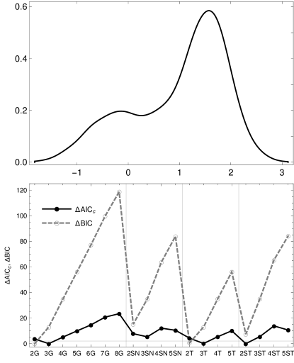
Figure 1: Histogram (top) and information criteria scores (bottom) for $\log T_{90}$.

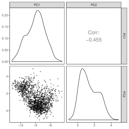
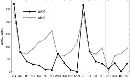
Figure 2: Scatter plots and histograms (top) and information criteria scores (bottom) for $PC_{1}-PC_{2}$.

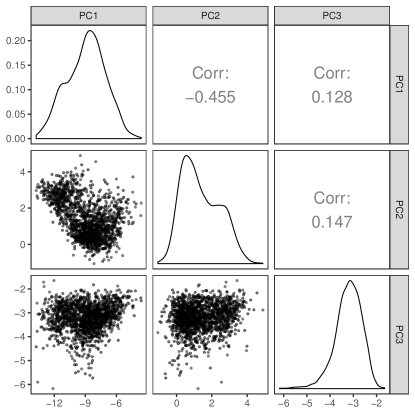
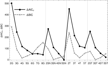
Figure 3: Scatter plots and histograms (top) and information criteria scores (bottom) for $PC_{1}-PC_{2}-PC_{3}$.

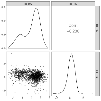
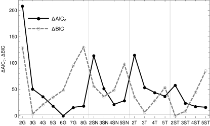
Figure 4: Scatter plots and histograms (top) and information criteria scores (bottom) for $\log T_{90}-\log H_{43}$.

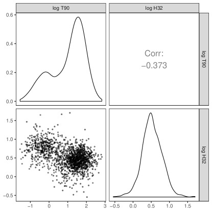
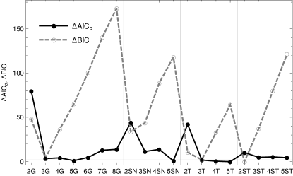
Figure 5: Scatter plots and histograms (top) and information criteria scores (bottom) for $\log T_{90}-\log H_{32}$.

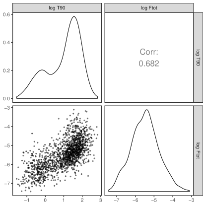
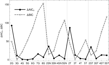
Figure 6: Scatter plots and histograms (top) and information criteria scores (bottom) for $\log T_{90}-\log F_{\rm tot}$ with $F_{4}\neq 0$.

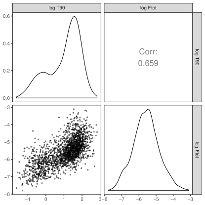
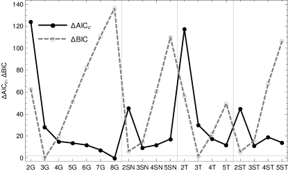
Figure 7: Scatter plots and histograms (top) and information criteria scores (bottom) for $\log T_{90}-\log F_{\rm tot}$ including $F_{4}=0$.

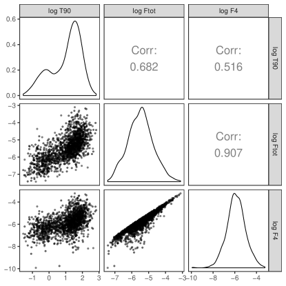
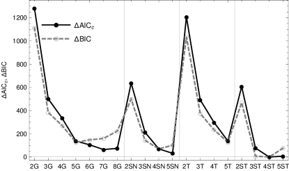
Figure 8: Scatter plots and histograms (top) and information criteria scores (bottom) for $\log T_{90}-\log F_{\rm tot}-\log F_{4}$.

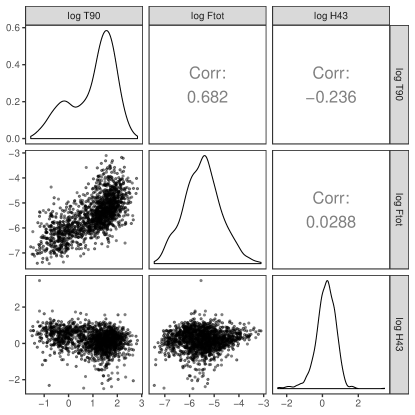
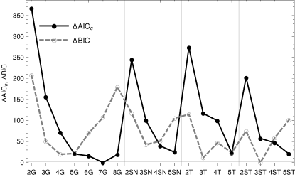
Figure 9: Scatter plots and histograms (top) and information criteria scores (bottom) for $\log T_{90}-\log F_{\rm tot}-\log H_{43}$.

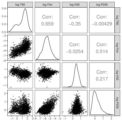
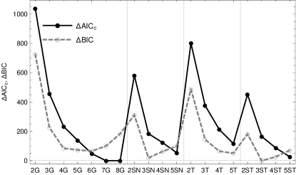
Figure 10: Scatter plots and histograms (top) and information criteria scores (bottom) for $\log T_{90}-\log F_{\rm tot}-\log H_{32}-\log P_{256}$.

Table 1: Best-fitting models (within $\Delta_{i}<2$).

Fig.	Data	Best models ($AIC_{c}$)	Best models ($BIC$)
1	$\log T_{90}$ (2037 GRBs)	2ST, 3G, 3T	2G, 2T
2	$PC_{1}-PC_{2}$ (1598 GRBs)	5SN, 4ST	2ST
3	$PC_{1}-PC_{2}-PC_{3}$ (1598 GRBs)	5SN	3ST, 3SN
4	$\log T_{90}-\log H_{43}$ (1598 GRBs)	6G	2ST
5	$\log T_{90}-\log H_{32}$ (1597 GRBs)	5T, 4T, 5SN, 5G, 3T	2ST
6	$\log T_{90}-\log F_{\rm tot}$ (1598 GRBs)	5G, 4G, 5T	3G, 3T
7	$\log T_{90}-\log F_{\rm tot}$ (1927 GRBs)	8G	3G, 3T
8	$\log T_{90}-\log F_{\rm tot}-\log F_{4}$ (1598 GRBs)	4ST	4ST
9	$\log T_{90}-\log F_{\rm tot}-\log H_{43}$ (1598 GRBs)	7G	3ST
10	$\log T_{90}-\log F_{\rm tot}-\log H_{32}-\log P_{256}$ (1927 GRBs)	7G, 8G	3ST

5 Discussion and summary

Multivariate modeling using skewed distributions was performed herein on the BATSE data set in various parameter spaces, ranging from the univariate $\log T_{90}$ case, through several two- and three-dimensional ones, e.g. spanned by the PCs, up to a four-dimensional $\log T_{90}-\log F_{\rm tot}-\log H_{32}-\log P_{256}$ instance (see Table 1). The six-dimensional case (Mukherjee et al., 1998; Chattopadhyay & Maitra, 2017; Tóth et al., 2019), i.e. with added $T_{50}$ and $H_{321}$, was not taken into account due to very high correlations ($r>0.96$) between $T_{90}$ and $T_{50}$, and between $H_{32}$ and $H_{321}$. To assess the goodnes-of-fit, information criteria ($AIC_{c}$ and $BIC$) were employed, and to validate the reliability of the inferences, a Monte Carlo benchmark test was done: it turned out that realizations of two-component mixtures of three-dimensional skewed distributions might be incorrectly recognized to come from a (spuriously) greater number of components. Additionally, $AIC_{c}$, due to its liberal tendency to overfit, has a higher chance of accepting more complex models, e.g. with redundant components, than necessary. Therefore, focus should be laid on interpreting the results via the values of $BIC$, which has a higher than $AIC_{c}$ probability of correctly assessing the fit. With that in mind, the key results can be summed up as follows:

1. the distribution of $\log T_{90}$ comprises of two components (supporting previous results: Tarnopolski 2016b; Kwong & Nadarajah 2018);

2. most two-dimensional instances are well described by two-component mixtures as well, except for those containing $F_{\rm tot}$, which yielded three-component symmetric fits (3G or 3T); in particular, previous results for the $\log T_{90}-\log H_{32}$ plane were confirmed (Tarnopolski, 2019a);

3. most three-dimensional spaces yielded mixtures of three skewed components, except for the case of $\log T_{90}-\log F_{\rm tot}-\log F_{4}$, for which both $AIC_{c}$ and $BIC$ pointed at 4ST. This result possibly comes from a very high correlation ($r=0.907$) between $\log F_{\rm tot}$ and $\log F_{4}$, making this result likely flawed. After dropping $F_{4}$, this reduces to analyzing the case of $\log T_{90}-\log F_{\rm tot}$;

4. the four-dimensional case of $\log T_{90}-\log F_{\rm tot}-\log H_{32}-\log P_{256}$ indicates the presence of three skewed components.

It therefore can not be undoubtfully concluded whether the BATSE sample consists of two or three groups, as the three-component fits can be spurious artifacts owing to the finiteness of the sample and, more importantly, to a particular realization of the random sample that lead to biased results. Also, spaces with higher dimensionality are more and more capacious, hence the identification of an excessive number of clusters might be more likely to happen, which appears to be the case here. Moreover, the distributions tested herein are in fact arbitrary, and the correct, underlying distribution, while inherently skewed, might be of a different shape. Henceforth, an exact derivation of the distributions of the variables of interest, starting from the univariate $\log T_{90}$ one, is desired, and expected to shed light on the issue. Also, as initially put forward by Tarnopolski (2019a), the redshift distribution might play a crucial role in explaining the observed skewness.

The nature of the putative intermediate GRBs is unclear. The overdensity, manifesting through emergence of a third component in the Gaussian mixture modeling, was considered previously to consist of X-ray flashes (Veres et al., 2010; Grupe et al., 2013), but this cannot be a universal explanation (Řípa & Mészáros, 2014, 2016) due to inconsistent hardness ratios of the presumed third groups in BATSE and RHESSI (Řípa et al. 2012; see also the discussion in Tarnopolski 2019a). As sGRBwEE are a plausible link between short and long GRBs (Kaneko et al., 2015), with their typical durations of $\sim 5-100\,{\rm s}$, they are attractive potential candidates for the intermediate group (see also Kann et al. 2011).

In the end, the existence of this elusive, third class of GRBs remains debatable. As implied by benchmark testing, and the inconsistency of the outcomes obtained for the various spaces examined herein, a phenomenological approach of fitting various distributions and seeking the best model does not provide unambiguous interpretations. In particular, very different fits, with the same goodness-of-fit measures, can be found for the same data (Koen & Bere, 2012). Due to the methodology of statistical inference, even finding a mixture with three (or more) components (including skewed) to be the best description of a given sample, is not decisive in asserting the number of physically valid GRB groups. Therefore it is very likely that there are still in fact only two main groups of GRBs. The excess, observed via skewness of one component or introduction of a third one, might be either a statistical artifact owing to e.g. selection effects, be a result of an inherently skewed distribution governing the prompt phase, or come from cosmological dilation stretching a Gaussian distribution into a skewed one. Even in parameter spaces of dimension greater than two, where the $BIC$ firmly implies three components, the results of the benchmark testing invoke a careful examination of all possiblities. On one hand, three components might become visible only in richer spaces; on the other, PCA suggests two dimensions should be enough, leading to a preference of two GRB classes rather than three.

References

- Abbott et al. (2017a) Abbott, B. P., Abbott, R., Abbott, T. D., et al. 2017a, ApJ, 848, L12, doi: 10.3847/2041-8213/aa91c9
- Abbott et al. (2017b) —. 2017b, ApJ, 848, L13, doi: 10.3847/2041-8213/aa920c
- Acuner & Ryde (2018) Acuner, Z., & Ryde, F. 2018, MNRAS, 475, 1708, doi: 10.1093/mnras/stx3106
- Akaike (1974) Akaike, H. 1974, IEEE Transactions on Automatic Control, 19, 716
- Bagoly et al. (2003) Bagoly, Z., Csabai, I., Mészáros, A., et al. 2003, A&A, 398, 919, doi: 10.1051/0004-6361:20021724
- Bagoly et al. (1998) Bagoly, Z., Mészáros, A., Horváth, I., Balázs, L. G., & Mészáros, P. 1998, ApJ, 498, 342, doi: 10.1086/305530
- Balastegui et al. (2001) Balastegui, A., Ruiz-Lapuente, P., & Canal, R. 2001, MNRAS, 328, 283, doi: 10.1046/j.1365-8711.2001.04888.x
- Balázs et al. (2003) Balázs, L. G., Bagoly, Z., Horváth, I., Mészáros, A., & Mészáros, P. 2003, A&A, 401, 129, doi: 10.1051/0004-6361:20021863
- Band et al. (1993) Band, D., Matteson, J., Ford, L., et al. 1993, ApJ, 413, 281, doi: 10.1086/172995
- Biesiada (2007) Biesiada, M. 2007, J. Cosmology Astropart. Phys, 2, 003, doi: 10.1088/1475-7516/2007/02/003
- Borgonovo & Björnsson (2006) Borgonovo, L., & Björnsson, C.-I. 2006, ApJ, 652, 1423, doi: 10.1086/508488
- Bostancı et al. (2013) Bostancı, Z. F., Kaneko, Y., & Göğüş, E. 2013, MNRAS, 428, 1623, doi: 10.1093/mnras/sts157
- Bromberg et al. (2011) Bromberg, O., Nakar, E., & Piran, T. 2011, ApJ, 739, L55, doi: 10.1088/2041-8205/739/2/L55
- Bromberg et al. (2013) Bromberg, O., Nakar, E., Piran, T., & Sari, R. 2013, ApJ, 764, 179, doi: 10.1088/0004-637X/764/2/179
- Burnham & Anderson (2004) Burnham, K. P., & Anderson, D. R. 2004, Sociological Methods & Research, 33, 261, doi: 10.1177/0049124104268644
- Bystřický et al. (2012) Bystřický, P., Mészáros, A., & Řípa, J. 2012, in Proceedings of the 21st Annual Conference of Doctoral Students - WDS 2012, Prague, 29th May - 1st June, 2012, Edited by Jana Šafránková and Jiří Pavlů, MATFYZPRESS, Prague, Part III - Physics, f-1
- Cano et al. (2017) Cano, Z., Wang, S.-W., Dai, Z.-G., & Wu, X.-F. 2017, Advances in Astronomy, 2017, 8929054
- Chattopadhyay & Maitra (2017) Chattopadhyay, S., & Maitra, R. 2017, MNRAS, 469, 3374, doi: 10.1093/mnras/stx1024
- Chattopadhyay & Maitra (2018) —. 2018, MNRAS, 481, 3196, doi: 10.1093/mnras/sty1940
- Dong et al. (2018) Dong, Y.-Z., Gu, W.-M., Liu, T., & Wang, J. 2018, MNRAS, 475, L101, doi: 10.1093/mnrasl/sly014
- Dunteman (1989) Dunteman, G. H. 1989, Quantitative Applications in the Social Sciences: Principal components analysis. (Newbury Park, CA: SAGE Publications, Inc.), doi: 10.4135/9781412985475
- Eichler et al. (1989) Eichler, D., Livio, M., Piran, T., & Schramm, D. N. 1989, Nature, 340, 126, doi: 10.1038/340126a0
- Filippenko (1997) Filippenko, A. V. 1997, ARA&A, 35, 309, doi: 10.1146/annurev.astro.35.1.309
- Fynbo et al. (2006) Fynbo, J. P. U., Watson, D., Thöne, C. C., et al. 2006, Nature, 444, 1047, doi: 10.1038/nature05375
- Galama et al. (1998) Galama, T. J., Vreeswijk, P. M., van Paradijs, J., et al. 1998, Nature, 395, 670, doi: 10.1038/27150
- Gendre et al. (2013) Gendre, B., Stratta, G., Atteia, J. L., et al. 2013, ApJ, 766, 30, doi: 10.1088/0004-637X/766/1/30
- Goldstein et al. (2017) Goldstein, A., Veres, P., Burns, E., et al. 2017, ApJ, 848, L14, doi: 10.3847/2041-8213/aa8f41
- Gruber et al. (2014) Gruber, D., Goldstein, A., Weller von Ahlefeld, V., et al. 2014, ApJS, 211, 12, doi: 10.1088/0067-0049/211/1/12
- Grupe et al. (2013) Grupe, D., Nousek, J. A., Veres, P., Zhang, B.-B., & Gehrels, N. 2013, ApJS, 209, 20, doi: 10.1088/0067-0049/209/2/20
- Hjorth et al. (2003) Hjorth, J., Sollerman, J., Møller, P., et al. 2003, Nature, 423, 847, doi: 10.1038/nature01750
- Horváth (1998) Horváth, I. 1998, ApJ, 508, 757, doi: 10.1086/306416
- Horváth (2002) —. 2002, A&A, 392, 791, doi: 10.1051/0004-6361:20020808
- Horváth et al. (2010) Horváth, I., Bagoly, Z., Balázs, L. G., et al. 2010, ApJ, 713, 552, doi: 10.1088/0004-637X/713/1/552
- Horváth et al. (2006) Horváth, I., Balázs, L. G., Bagoly, Z., Ryde, F., & Mészáros, A. 2006, A&A, 447, 23, doi: 10.1051/0004-6361:20041129
- Horváth et al. (2008) Horváth, I., Balázs, L. G., Bagoly, Z., & Veres, P. 2008, A&A, 489, L1, doi: 10.1051/0004-6361:200810269
- Horváth et al. (2012) Horváth, I., Balázs, L. G., Hakkila, J., Bagoly, Z., & Preece, R. D. 2012, in Gamma-Ray Bursts 2012 Conference (GRB 2012), 46
- Horváth et al. (2018) Horváth, I., Tóth, B. G., Hakkila, J., et al. 2018, Ap&SS, 363, 53, doi: 10.1007/s10509-018-3274-5
- Huja et al. (2009) Huja, D., Mészáros, A., & Řípa, J. 2009, A&A, 504, 67, doi: 10.1051/0004-6361/200809802
- Hurley et al. (2010) Hurley, K., Rowlinson, A., Bellm, E., et al. 2010, MNRAS, 403, 342, doi: 10.1111/j.1365-2966.2009.16118.x
- Hurvich & Tsai (1989) Hurvich, C. M., & Tsai, C.-L. 1989, Biometrika, 76, 297
- Kagawa et al. (2019) Kagawa, Y., Yonetoku, D., Sawano, T., et al. 2019, ApJ, 877, 147, doi: 10.3847/1538-4357/ab1bd6
- Kaneko et al. (2015) Kaneko, Y., Bostancı, Z. F., Göğüş, E., & Lin, L. 2015, MNRAS, 452, 824, doi: 10.1093/mnras/stv1286
- Kann et al. (2011) Kann, D. A., Klose, S., Zhang, B., et al. 2011, ApJ, 734, 96, doi: 10.1088/0004-637X/734/2/96
- Kass & Raftery (1995) Kass, R. E., & Raftery, A. E. 1995, J. Am. Stat. Assoc., 90, 773
- King et al. (2007) King, A., Olsson, E., & Davies, M. B. 2007, MNRAS, 374, L34, doi: 10.1111/j.1745-3933.2006.00259.x
- Klebesadel et al. (1973) Klebesadel, R. W., Strong, I. B., & Olson, R. A. 1973, ApJ, 182, L85, doi: 10.1086/181225
- Koen & Bere (2012) Koen, C., & Bere, A. 2012, MNRAS, 420, 405, doi: 10.1111/j.1365-2966.2011.20045.x
- Koshut et al. (1996) Koshut, T. M., Paciesas, W. S., Kouveliotou, C., et al. 1996, ApJ, 463, 570, doi: 10.1086/177272
- Kouveliotou et al. (1993) Kouveliotou, C., Meegan, C. A., Fishman, G. J., et al. 1993, ApJ, 413, L101, doi: 10.1086/186969
- Kulkarni & Desai (2017) Kulkarni, S., & Desai, S. 2017, Ap&SS, 362, 70, doi: 10.1007/s10509-017-3047-6
- Kwong & Nadarajah (2018) Kwong, H. S., & Nadarajah, S. 2018, MNRAS, 473, 625, doi: 10.1093/mnras/stx2373
- Lazzati et al. (2005) Lazzati, D., Ghirlanda, G., & Ghisellini, G. 2005, MNRAS, 362, L8, doi: 10.1111/j.1745-3933.2005.00062.x
- Levan et al. (2014) Levan, A. J., Tanvir, N. R., Starling, R. L. C., et al. 2014, ApJ, 781, 13, doi: 10.1088/0004-637X/781/1/13
- Li et al. (2016) Li, Y., Zhang, B., & Lü, H.-J. 2016, ApJS, 227, 7, doi: 10.3847/0067-0049/227/1/7
- Liddle (2007) Liddle, A. R. 2007, MNRAS, 377, L74, doi: 10.1111/j.1745-3933.2007.00306.x
- Lien et al. (2016) Lien, A., Sakamoto, T., Barthelmy, S. D., et al. 2016, ApJ, 829, 7, doi: 10.3847/0004-637X/829/1/7
- MacFadyen & Woosley (1999) MacFadyen, A. I., & Woosley, S. E. 1999, ApJ, 524, 262, doi: 10.1086/307790
- Mazets et al. (1981) Mazets, E. P., Golenetskii, S. V., Ilinskii, V. N., et al. 1981, Ap&SS, 80, 3, doi: 10.1007/BF00649140
- McBreen et al. (1994) McBreen, B., Hurley, K. J., Long, R., & Metcalfe, L. 1994, MNRAS, 271, 662, doi: 10.1093/mnras/271.3.662
- Meegan et al. (1992) Meegan, C. A., Fishman, G. J., Wilson, R. B., et al. 1992, Nature, 355, 143, doi: 10.1038/355143a0
- Mukherjee et al. (1998) Mukherjee, S., Feigelson, E. D., Jogesh Babu, G., et al. 1998, ApJ, 508, 314, doi: 10.1086/306386
- Nakar (2007) Nakar, E. 2007, Phys. Rep., 442, 166, doi: 10.1016/j.physrep.2007.02.005
- Narayan et al. (1992) Narayan, R., Paczyński, B., & Piran, T. 1992, ApJ, 395, L83, doi: 10.1086/186493
- Narayana Bhat et al. (2016) Narayana Bhat, P., Meegan, C. A., von Kienlin, A., et al. 2016, ApJS, 223, 28, doi: 10.3847/0067-0049/223/2/28
- Norris & Bonnell (2006) Norris, J. P., & Bonnell, J. T. 2006, ApJ, 643, 266, doi: 10.1086/502796
- Ofek (2007) Ofek, E. O. 2007, ApJ, 659, 339, doi: 10.1086/511147
- Ofek et al. (2008) Ofek, E. O., Muno, M., Quimby, R., et al. 2008, ApJ, 681, 1464, doi: 10.1086/587686
- Ohmori et al. (2016) Ohmori, N., Yamaoka, K., Ohno, M., et al. 2016, PASJ, 68, S30, doi: 10.1093/pasj/psw009
- Paciesas et al. (1999) Paciesas, W. S., Meegan, C. A., Pendleton, G. N., et al. 1999, ApJS, 122, 465, doi: 10.1086/313224
- Paczyński (1991) Paczyński, B. 1991, Acta Astron., 41, 257
- Paczyński (1998) Paczyński, B. 1998, ApJ, 494, L45, doi: 10.1086/311148
- Pendleton et al. (1997) Pendleton, G. N., Paciesas, W. S., Briggs, M. S., et al. 1997, ApJ, 489, 175, doi: 10.1086/304763
- Perna et al. (2018) Perna, R., Lazzati, D., & Cantiello, M. 2018, ApJ, 859, 48, doi: 10.3847/1538-4357/aabcc1
- Prates et al. (2013) Prates, M., Lachos, V., & Cabral, C. B. 2013, Journal of Statistical Software, Articles, 54, 1, doi: 10.18637/jss.v054.i12
- Ruffini et al. (2018) Ruffini, R., Wang, Y., Aimuratov, Y., et al. 2018, ApJ, 852, 53, doi: 10.3847/1538-4357/aa9e8b
- Savchenko et al. (2017) Savchenko, V., Ferrigno, C., Kuulkers, E., et al. 2017, ApJ, 848, L15, doi: 10.3847/2041-8213/aa8f94
- Schwarz (1978) Schwarz, G. 1978, Ann. Statist., 6, 461, doi: 10.1214/aos/1176344136
- Stanek et al. (2003) Stanek, K. Z., Matheson, T., Garnavich, P. M., et al. 2003, ApJ, 591, L17, doi: 10.1086/376976
- Svinkin et al. (2016) Svinkin, D. S., Frederiks, D. D., Aptekar, R. L., et al. 2016, ApJS, 224, 10, doi: 10.3847/0067-0049/224/1/10
- Tanvir et al. (2013) Tanvir, N. R., Levan, A. J., Fruchter, A. S., et al. 2013, Nature, 500, 547, doi: 10.1038/nature12505
- Tarnopolski (2015a) Tarnopolski, M. 2015a, Ap&SS, 359, 20, doi: 10.1007/s10509-015-2473-6
- Tarnopolski (2015b) —. 2015b, A&A, 581, A29, doi: 10.1051/0004-6361/201526415
- Tarnopolski (2016a) —. 2016a, New A, 46, 54, doi: 10.1016/j.newast.2015.12.006
- Tarnopolski (2016b) —. 2016b, MNRAS, 458, 2024, doi: 10.1093/mnras/stw429
- Tarnopolski (2016c) —. 2016c, Ap&SS, 361, 125, doi: 10.1007/s10509-016-2687-2
- Tarnopolski (2019a) —. 2019a, ApJ, 870, 105, doi: 10.3847/1538-4357/aaf1c5
- Tarnopolski (2019b) —. 2019b, arXiv e-prints, arXiv:1907.00355. https://arxiv.org/abs/1907.00355
- Tóth et al. (2019) Tóth, B. G., Rácz, I. I., & Horváth, I. 2019, MNRAS, 486, 4823, doi: 10.1093/mnras/stz1188
- Tsutsui et al. (2013) Tsutsui, R., Nakamura, T., Yonetoku, D., Takahashi, K., & Morihara, Y. 2013, PASJ, 65, 3, doi: 10.1093/pasj/65.1.3
- Tsutsui & Shigeyama (2014) Tsutsui, R., & Shigeyama, T. 2014, PASJ, 66, 42, doi: 10.1093/pasj/psu008
- Řípa & Mészáros (2014) Řípa, J., & Mészáros, A. 2014, in Proceedings of Swift: 10 Years of Discovery (SWIFT 10), held 2-5 December 2014 at La Sapienza University, Rome, Italy. id.103, 103
- Řípa & Mészáros (2016) Řípa, J., & Mészáros, A. 2016, Ap&SS, 361, 370, doi: 10.1007/s10509-016-2960-4
- Řípa et al. (2012) Řípa, J., Mészáros, A., Veres, P., & Park, I. H. 2012, ApJ, 756, 44, doi: 10.1088/0004-637X/756/1/44
- Řípa et al. (2009) Řípa, J., Mészáros, A., Wigger, C., et al. 2009, A&A, 498, 399, doi: 10.1051/0004-6361/200810913
- Veres et al. (2010) Veres, P., Bagoly, Z., Horváth, I., Mészáros, A., & Balázs, L. G. 2010, ApJ, 725, 1955, doi: 10.1088/0004-637X/725/2/1955
- von Kienlin et al. (2014) von Kienlin, A., Meegan, C. A., Paciesas, W. S., et al. 2014, ApJS, 211, 13, doi: 10.1088/0067-0049/211/1/13
- Wang et al. (2019) Wang, F., Zou, Y.-C., Liu, F., et al. 2019, arXiv e-prints, arXiv:1902.05489. https://arxiv.org/abs/1902.05489
- Woosley (1993) Woosley, S. E. 1993, ApJ, 405, 273, doi: 10.1086/172359
- Woosley & Bloom (2006) Woosley, S. E., & Bloom, J. S. 2006, ARA&A, 44, 507, doi: 10.1146/annurev.astro.43.072103.150558
- Yang et al. (2016) Yang, E. B., Zhang, Z. B., & Jiang, X. X. 2016, Ap&SS, 361, 257, doi: 10.1007/s10509-016-2838-5
- Zhang et al. (2014) Zhang, B.-B., Zhang, B., Murase, K., Connaughton, V., & Briggs, M. S. 2014, ApJ, 787, 66, doi: 10.1088/0004-637X/787/1/66
- Zhang & Choi (2008) Zhang, Z.-B., & Choi, C.-S. 2008, A&A, 484, 293, doi: 10.1051/0004-6361:20079210
- Zhang et al. (2016) Zhang, Z.-B., Yang, E.-B., Choi, C.-S., & Chang, H.-Y. 2016, MNRAS, 462, 3243, doi: 10.1093/mnras/stw1835
- Zitouni et al. (2018) Zitouni, H., Guessoum, N., AlQassimi, K. M., & Alaryani, O. 2018, Ap&SS, 363, 223, doi: 10.1007/s10509-018-3449-0
- Zitouni et al. (2015) Zitouni, H., Guessoum, N., Azzam, W. J., & Mochkovitch, R. 2015, Ap&SS, 357, 7, doi: 10.1007/s10509-015-2311-x