A Unified Contraction Analysis of a Class of Distributed Algorithms for Composite Optimization

Abstract

We study distributed composite optimization over networks: agents minimize the sum of a smooth (strongly) convex function–the agents’ sum-utility–plus a nonsmooth (extended-valued) convex one. We propose a general algorithmic framework for such a class of problems and provide a unified convergence analysis leveraging the theory of operator splitting. Our results unify several approaches proposed in the literature of distributed optimization for special instances of our formulation. Distinguishing features of our scheme are: (i) when the agents’ functions are strongly convex, the algorithm converges at a linear rate, whose dependencies on the agents’ functions and the network topology are decoupled, matching the typical rates of centralized optimization; (ii) the step-size does not depend on the network parameters but only on the optimization ones; and (iii) the algorithm can adjust the ratio between the number of communications and computations to achieve the same rate of the centralized proximal gradient scheme (in terms of computations). This is the first time that a distributed algorithm applicable to composite optimization enjoys such properties.

I Introduction

We study distributed multi-agent optimization over networks, modeled as undirected static graphs. Agents aim at solving

$$\min_{x\in\mathbb{R}^{d}}F(x)+G(x),\quad F(x)\triangleq{\frac{1}{m}}\sum_{i=1}^{m}f_{i}(x),\vspace{-0.1cm}$$ (P)

where $f_{i}:\mathbb{R}^{d}\to\mathbb{R}$ is the cost-function of agent $i$, assumed to be smooth, (strongly) convex and known only to the agent; and $G:\mathbb{R}^{d}\to\mathbb{R}\cup\{-\infty,\infty\}$ is a nonsmooth, convex (extended-value) function, which can be used to enforce shared constraints or some specific structure on the solution, such as sparsity.
Our focus is on the design of distributed algorithms for Problem (P) that provably converge at a linear rate. When $G=0$, several distributed schemes have been proposed in the literature enjoying such a property; examples include EXTRA [1], AugDGM [2], NEXT [3], SONATA [4, 5], DIGing [6], NIDS [7], Exact Diffusion [8], MSDA [9], and the distributed algorithms in [10],[11], and [12]. When $G\neq 0$ results are scarce; to our knowledge, the only two schemes available in the literature achieving linear rate for (P) are SONATA [5] and the distributed proximal gradient algorithm [13]. The aforementioned algorithms apparently look different; no unified convergence analysis can be inferred; and, in most of the cases, step-size bounds and convergence rate seem quite conservative. This naturally suggests the following two questions:

• Can one unify the design and analysis of distributed algorithms in the setting (P)?

• Can one match the linear convergence rate of the centralized proximal-gradient algorithm applied to (P)?

Recent efforts toward a better understanding of the taxonomy of distributed algorithms (question Q1) are the following: [11] provides a connection between EXTRA and DIGing; [14] provides a canonical representation of some of the distributed algorithms above–NIDS and Exact-Diffusion are proved to be equivalent; and [15] provide an automatic (numerical) procedure to prove linear rate of some classes of distributed algorithms. These efforts model only first order algorithms applicable to Problem (P) with $G=0$ and employing a single round of communication and gradient computation. Because of that, in general, they cannot achieve the rate of the centralized gradient algorithm (addressing thus Q2). Works partially addressing Q2 are the following: MSDA [9] uses multiple communication steps to achieve the lower complexity bound of (P) when $G=0$; and the algorithms in [16] and [7] achieve linear rate and can adjust the number of communications performed at each iteration to match the rate of the centralized gradient descent. However it is not clear how to extend (if possible) these methods and their convergence analysis to the more general composite (i.e., $G\neq 0$) setting (P).
This paper aims at addressing Q1 and Q2 in the general setting (P). Our major contributions are the following: 1) We propose a general primal-dual distributed algorithmic framework that subsumes several existing ATC- and CTA-based distributed algorithms; 2) A sharp linear convergence rate is proved (when $G\neq 0$) developing an operator contraction-based analysis. By product, our convergence results apply also to the algorithms in [1, 7, 8, 10, 3, 2], which so far have been studied in isolation; 3) For ATC forms of our schemes, the dependencies of the linear rate on the agents’ functions and the network topology are decoupled, matching the typical rates for the centralized optimization and the consensus averaging. This is a major departure from existing analyses, which do not show such a clear separation, and complements the results in [7] applicable only to smooth instances of (P). Furthermore, convergence is established under a proper choice of the step-size, whose upper bound does not depend on the network parameters but only on the optimization ones (Lipschitz constants of the gradients and strongly convexity constants); and 4) The proposed scheme can naturally adjusts the ratio between the number of communications and computations to achieve the same rate of the centralized proximal gradient scheme (in terms of computations). Chebyshev acceleration can also be employed to significantly reduce the number of communication steps per computation. Because of space limitation, all the proofs are available as supporting material in the technical report [17].
Notations: $\mathbb{N}_{+}$ is the set of positive integer numbers; $\mathbb{S}^{m}$ is the set of $\mathbb{R}^{m\times m}$ symmetric matrices while $\mathbb{S}_{+}^{m}$ (resp. $\mathbb{S}_{++}^{m}$) is the set of positive semidefinite (resp. definite) matrices in $\mathbb{S}^{m}$. $\mathbb{P}_{K}$ denotes the set of (real) monic polynomials of order $K$. Unless otherwise indicated, column vectors are denoted by lower-case letters while upper-case letters are used for matrices (with the exception of $L$ in Assumption 1 to conform with conventional notation). The symbols $1_{m}$ and $0_{m}$ denote the $m$-length column vectors of all ones and all zeros, respectively. The $\mathbf{0}_{m}$ denotes the $m\times m$ zero matrix; $I_{m}$ denotes the identity matrix in $\mathbb{R}^{m\times m}$; $J\triangleq 1_{m}\,1_{m}^{\top}/m$ is the projection matrix onto $1_{m}$. With a slight abuse of notation, $I$ will denote either the identity matrix or the identity operator on the space under consideration. We use ${\texttt{null}}(\cdot)$ [resp. ${\texttt{span}}(\cdot)$] to denote the null space (resp. range space) of the matrix argument. For any $X,Y\in\mathbb{R}^{m\times d}$, let $\left\langle X,Y\right\rangle\triangleq\text{trace}(X^{\top}Y)$ while we write $\left\|X\right\|$ for $\left\|X\right\|_{F}$; the same notation is used for vectors, treated as special cases. Given ${G}\in\mathbb{S}_{+}^{n}$, $\left\langle X,Y\right\rangle_{G}\triangleq\left\langle GX,Y\right\rangle$ and $\left\|X\right\|_{G}\triangleq\sqrt{\left\langle X,X\right\rangle_{G}}.$ The eigenvalues of a symmetric matrix ${A}\in\mathbb{R}^{m\times m}$ are denoted by $\lambda_{i}(A)$, $i=1,\ldots,m$, and arranged in increasing order. For $x\in\mathbb{R},$ we denote $x_{+}=\max(x,0).$

II Problem Statement

We study Problem (P) under the following assumption.

Assumption 1.

Each local cost function $f_{i}:\mathbb{R}^{d}\rightarrow\mathbb{R}$ is $\mu$-strongly convex and $L$-smooth; and $G:\mathbb{R}^{d}\rightarrow\mathbb{R}\cup\{\pm\infty\}$ is proper, closed and convex. Define $\kappa\triangleq L/\mu$.

Note that Assumption 1 also accounts for the case where $f_{i}$ is convex and $G$ is $\mu$-strongly convex.
Network model: Agents are embedded in a network, modeled as an undirected, static graph $\mathcal{G}=(\mathcal{V},\mathcal{E})$, where $\mathcal{V}$ is the set of nodes (agents) and $\{i,j\}\in\mathcal{E}$ if there is an edge (communication link) between node $i$ and $j$. We make the blanket assumption that $\mathcal{G}$ is connected. We introduce the following matrices associated with $\mathcal{G}$, which will be used to build the proposed distributed algorithms.

Definition 1 (Gossip matrix).

A matrix $W\triangleq[W_{ij}]\in\mathbb{R}^{m\times m}$ is said to be compliant to the graph $\mathcal{G}=(\mathcal{V},\mathcal{E})$ if $W_{ij}\neq 0$ for $\{i,j\}\in\mathcal{E}$, and $W_{ij}=0$ otherwise. The set of such matrices is denoted by $\mathcal{W}_{\mathcal{G}}$.

Definition 2 ($K$-hop gossip matrix).

Given $K\in\mathbb{N}_{+},$ a matrix ${W}^{\prime}\in\mathbb{R}^{m\times m}$ is said to be a $K$-hop gossip matrix associated to $\mathcal{G}=(\mathcal{V},\mathcal{E})$ if ${W}^{\prime}=P_{K}(W)$, for some $W\in\mathcal{W}_{\mathcal{G}}$, where $P_{K}(\cdot)\in\mathbb{P}_{K}$.

Note that, if $W\in\mathcal{W}_{\mathcal{G}}$, using $W_{ij}$ to linearly combine information between agent $i$ and $j$ corresponds to performing a single communication between the two agents ($i$ and $j$ are immediate neighbors). Using a $K$-hop matrix ${W}^{\prime}=P_{K}(W)$ requires instead $K$ consecutive rounds of communications among immediate neighbors for the aforementioned weighting process to be implemented in a distributed way (note that the zero-pattern of ${W}^{\prime}$ is in general not compliant with $\mathcal{G}$). $K$-hop weight matrices are crucial to employ acceleration of the communication step, which will be a key ingredient to exploit the tradeoff between communications and computations (cf. Sec. V).
A saddle-point reformulation: Our path to design distributed solution methods for (P) is to solve a saddle-point reformulation of (P) via general proximal splitting algorithms that are implementable over $\mathcal{G}$. Following a standard path in the literature, we introduce local copies $x_{i}\in\mathbb{R}^{d}$ (the $i$-th one is owned by agent $i$) of $x$ and functions

$$f(X)\triangleq\sum_{i=1}^{m}f_{i}(x_{i})\quad\text{and}\quad g(X)\triangleq\sum_{i=1}^{m}G(x_{i}),\vspace{-0.1cm}$$ (1)

with $X\triangleq[x_{1},\ldots,x_{m}]^{\top}\in\mathbb{R}^{m\times d}$; (P) can be then rewritten as

$$\min_{X\in\mathbb{R}^{m\times d}}f(X)+g(X),~{}{\text{s.t.}}~{}\sqrt{{C}}X=\mathbf{0},\vspace{-0.1cm}$$ (2)

where $C$ satisfies the following assumption:

Assumption 2.

$C\in\mathbb{S}^{m}_{+}$ and ${\texttt{null}}({C})={\texttt{span}}(1)$.

Under this condition, the constraint $\sqrt{{C}}X=\mathbf{0}$ enforces a consensus among $x_{i}$’s and thus (2) is equivalent to (P).
In the setting above, (2) is equivalent to its KKT conditions: there exists $X^{\star}\in\mathcal{S}_{\text{KKT}}$, where $\mathcal{S}_{\text{KKT}}$ is defined as

$$\mathcal{S}_{\texttt{KKT}}\triangleq \left\{X\in\mathbb{R}^{m\times d}\,\big{|}\,\exists\,Y\in\mathbb{R}^{m\times d}\text{ such that}\right.$$

$$\left.\sqrt{{C}}X=\mathbf{0},\quad\nabla f(X)+\sqrt{{C}}Y\in-\partial g(X)\right\},$$ (3)

where $\nabla f(X)\triangleq[\nabla f_{1}(x_{1}),\nabla f_{2}(x_{2}),...,\nabla f_{m}(x_{m})]^{\top}$ and $\partial g(X)$ denotes the subdifferential of $g$ at $X$. We have the following.

Lemma 1.

Consider Problem (P) under Assumptions 1 and 2; $x^{\star}\in\mathbb{R}^{d}$ is an optimal solution of (P) if and only if ${1}_{m}x^{\star\top}\in\mathcal{S}_{\texttt{KKT}}$.

Building on Lemma 1, in the next section, we propose a general distributed algorithm for (P) based on a suitably defined operator splitting solving the KKT system (II).

III A General Primal-Dual Proximal Algorithm

The proposed general primal-dual proximal algorithm reads

$$X^{k} =\text{prox}_{\gamma g}\left(Z^{k}\right),$$ (4a)

$$Z^{k+1} =AX^{k}-\gamma B\nabla f(X^{k})-Y^{k},$$ (4b)

$$Y^{k+1} =Y^{k}+{C}Z^{k+1},$$ (4c)

with $Z^{0}\in\mathbb{R}^{m\times d}$ and $Y^{0}\in{\texttt{span}}({C})$. In (4a), $\text{prox}_{\gamma g}\left(X\right)\triangleq\text{arg}\min_{Y}g(Y)+\frac{1}{2\gamma}\left\|X-Y\right\|^{2}$ is the standard proximal operator, which accounts for the nonsmooth term. Eq. (4a) represents the update of the primal variables, where $A,B\in\mathbb{R}^{m\times m}$ are suitably chosen weight matrices, and $\gamma>0$ is the step-size. Finally, (4c) represents the update of the dual variables. Note that there is no loss of generality in initializing $Y^{0}\in{\texttt{span}}({C})$, as any $Y$ in (II) is so (unless all the $f_{i}$ share a common minimizer).
Define the set $\mathcal{S}_{\texttt{Fix}}\triangleq\big{\{}X\in\mathbb{R}^{m\times d}\,\big{|}\,CX=0\text{ and }1^{\top}(I-A)X+\gamma\,1^{\top}B\nabla f(X)\in-\gamma\,1^{\top}\partial g(X)\big{\}}$. It is not difficult to check that any fixed point $(X^{\star},Z^{\star},Y^{\star})$ of Algorithm (4) satisfies $X^{\star}\in\mathcal{S}_{\texttt{Fix}}$. The following are necessary and sufficient conditions on $A$ and $B$ for $X^{\star}\in\mathcal{S}_{\texttt{Fix}}$ to be the solution of (2).

Assumption 3.

The weight matrices $A,B\in\mathbb{R}^{m\times m}$ satisfy: $1^{\top}A\,1=m$, and $1^{\top}B=1^{\top}$.

Lemma 2 (​[17]).

Under Assumption 2, $\mathcal{S}_{\texttt{KKT}}=\mathcal{S}_{\texttt{Fix}}$ if and only if $A,B$ satisfy Assumption 3.

III-A Connections with existing distributed algorithms

Algorithm (4) contains a gamut of distributed (and centralized) schemes, corresponding to different choices of the weight matrices $A,B,$ and $C$; any $A,B,C\in\mathcal{W}_{\mathcal{G}}$ leads to distributed implementations. The use of general matrices $A$ and $B$ (rather the more classical choices $A=B$ or $B=I$) permits to model for the first time in a unified algorithmic framework both ATC- and CTA-based updates; this includes several existing distributed algorithms proposed for special cases of (P), as briefly discussed next; see [17] for more examples. Rewrite Algorithm (4) in the following equivalent form:

$$Z^{k+2}=(I-C)Z^{k+1}+A(X^{k+1}-X^{k})-\gamma B(\nabla f(X^{k+1})-\nabla f(X^{k})).\vspace{-0.2cm}$$ (5)

When $G=0$, the above update reduces to

$$X^{k+2}=(I-C+A)X^{k+1}-AX^{k}-\gamma B(\nabla f(X^{k+1})-\nabla f(X^{k})).\vspace{-0.1cm}$$ (6)

It is not difficult to check that the schemes in [1, 7, 8, 3, 2, 6, 10, 11, 12, 13] are all special cases of (5) or (6) and thus of Algorithm (4)–Table I shows the proper parameter setting to establish the equivalence, where $W\in\mathcal{W}_{\mathcal{G}}$ is the weight matrix used in the target distributed algorithms, see [17] for more details.

Algorithm	$A~{}~{}|~{}~{}B~{}~{}|~{}~{}C$
EXTRA [1]	$\frac{1}{2}(I+W)~{}~{}|~{}~{}I~{}~{}|~{}~{}\frac{1}{2}(I-W)$
NIDS [7]/Exact Diffusion [8]	$\frac{1}{2}(I+W)~{}~{}|~{}~{}\frac{1}{2}(I+W)~{}~{}|~{}~{}\frac{1}{2}(I-W)$
NEXT [3]/AugDGM [2]	$W^{2}~{}~{}|~{}~{}W^{2}~{}~{}|~{}~{}(I-W)^{2}$
DIGing [6]/ [10]	$W^{2}~{}~{}|~{}~{}I~{}~{}|~{}~{}(I-W)^{2}$
[11]	$bW^{2}+(1-b)W~{}~{}|~{}~{}I~{}~{}|~{}~{}bW^{2}-(1+b)W+I$
[12]	$W^{K}~{}~{}|~{}~{}\sum_{i=1}^{K-1}{W^{i}}~{}~{}|~{}~{}W-W^{K}$
[13] ($G\neq 0$)	$W~{}~{}|~{}~{}I~{}~{}|~{}~{}\alpha(I-W)$

TABLE I: Connections with existing distributed algorithms. All the schemes but ours and [13] apply only to (P) with $G=0$.

IV Convergence Analysis

We establish linear rate of Algorithm (4) under the following assumption (along with Assumption 3).

Assumption 4.

The weight matrices $A\in\mathbb{R}^{m\times m},\,{B\in\mathbb{S}^{m}}$ and $C\in\mathbb{S}_{+}^{m}$ satisfy: i) $A=BD$ for some $-I\prec D\preceq I$; ii) $0\prec I-C$; iii) $B$ and $C$ commute; and iv) $B^{2}\prec\frac{(L+\mu)^{2}}{\left(L\lambda_{\text{max}}(D)-\mu\lambda_{\text{min}}(D)\right)^{2}}(I-C)$.

Assumption 4 together with Assumption 3 are quite mild and satisfied by a variety of algorithms; for instance, this is the case for all the schemes in Table I (see [17] for more details). In particular, the commuting property is trivially satisfied when $B,C\in P_{K}(W)$, for some given $W\in\mathcal{W}_{\mathcal{G}}$ (as in Table I). Also, one can show that condition iv) is necessary to achieve linear rate.

Theorem 3.

Consider Problem (P) under Assumption 1, whose optimal solution is $x^{\star}$. Let $\{(X^{k},Z^{k},Y^{k})\}_{k\geq 0}$ be the sequence generated by Algorithm (4) under Assumptions 2 and 3 and step-size

$$\frac{1}{\mu}\left(\lambda_{\max}(D)-\lambda_{\max}\left(B^{2}(I-C)^{-1}\right)^{-{1}/{2}}\right)_{+}<\gamma$$

$$\quad<\frac{1}{L}\left(\lambda_{\min}(D)+\lambda_{\max}\left(B^{2}(I-C)^{-1}\right)^{-{1}/{2}}\right).$$

Then $\left\|X^{k}-1x^{\star\top}\right\|^{2}=\mathcal{O}(\lambda^{k})$, with

$$\lambda\triangleq\max\left(q^{2}\lambda_{\max}(B^{2}(I-C)^{-1}),~{}1-\lambda_{2}(C)\right)<1,\vspace{-0.3cm}$$ (7)

and

$$q\triangleq \max\left(\left|\lambda_{\min}(D)-\gamma L\right|,~{}\left|\lambda_{\max}(D)-\gamma\mu\right|\right).$$ (8)

The optimal step-size is $\gamma^{\star}\triangleq\frac{\lambda_{\max}(D)+\lambda_{\min}(D)}{L+\mu}$ leading to the smallest $q^{\star}\triangleq\frac{L\lambda_{\max}(D)-\mu\lambda_{\min}(D)}{L+\mu}$, and thus the optimal rate.

Corollary 4.

Under the same setting as Theorem 3, let $B^{2}\preceq I-C$ and $A=B$, so that $D=I,~{}\gamma^{\star}=\frac{2}{L+\mu}$. Then, the rate reduces to

$$\lambda=\max\left\{\left(\frac{\kappa-1}{\kappa+1}\right)^{2},~{}1-\lambda_{2}(C)\right\}.\vspace{-0.2cm}$$ (9)

Note that the lower bound condition on the step-size in Theorem 3 nulls when $B^{2}(I-C)^{-1}\preceq I$ (since $\lambda_{\max}(D)=1$). Theorem 3 and Corollary 4 provide a unified set of convergence conditions for CTA- and ATC-based distributed algorithms. We refer to [17] for a detailed discussion of several special instances. Here, we mainly comment Algorithm (4) in the setting of Corollary 4. This special instance enjoys two desirable properties, namely: (i) rate-separation: The rate (9) is determined by the worst rate between the one due to the communication $[1-\lambda_{2}(C)]$ and that of the optimization $[((\kappa-1)/(\kappa+1))^{2}]$. This separable structure is the key enabler for our distributed scheme to achieve the convergence rate of the centralized proximal gradient algorithm applied to Problem (P)–see Sec. V; and (ii) network-independent step-size: The step-size in Corollary 4 does not depend on the network parameters but only on the optimization and its value coincides with the optimal step-size of the centralized proximal-gradient algorithm. This is a major advantage over current distributed schemes applicable to (P) (with $G\neq 0$) and complements the results in [7], whose algorithm however cannot deal with the non-smooth term $G$ and use a non-optimal step-size.

V Communication and computation trade-off

In this section we build on the rate separation property in Corollary 4 to show how to choose the matrices $A,\,B$ and $C$ to achieve the same rate of the centralized proximal gradient algorithm, possibly using multiple (finite) rounds of communications.
Note that $\rho_{\texttt{opt}}\triangleq(\kappa-1)/(\kappa+1)$ is the rate of the centralized proximal-gradient algorithm applied to Problem (P), under Assumption 1. This means that if the network is “well connected”, specifically $1-\lambda_{2}(C)\leq\rho_{\texttt{opt}}^{2}$, the proposed algorithm with the choice of $A,\,B$ and $C$ under consideration already converges at the desired linear rate $\rho_{\texttt{opt}}$. On the other hand, when $1-\lambda_{2}(C)>\rho_{\texttt{opt}}^{2}$, one can still achieve the centralized rate $\rho_{\texttt{opt}}$ by enabling multiple (finite) rounds of communications per proximal gradient evaluations. We discuss next two strategies to reach this goal, namely: 1) performing multiple rounds of plain consensus using each time the same weight matrix; and 2) employing acceleration via Chebyshev polynomials.
1) Multiple rounds of consensus: Given a weight matrix $W\in\mathcal{W}_{\mathcal{G}}$ (i.e., compatible with $\mathcal{G}$), we consider two possible choices of $A,B,C$ satisfying Corollary 4 and leading to distributed algorithms. Case 1: Suppose $W\in\mathbb{S}^{m}_{++}$. We set $A=B=I-C=W$, which implies $B^{2}\preceq I-C$ (cf. Corollary 4). The resulting algorithm implemented using (5) or (6) will require one communication exchange per gradient evaluation. Note that this setting subsumes most existing primal-dual methods such as NIDS [7]/Exact Diffusion [8]. If $W$ in the setting above is replaced by $W^{K}$, with $K>1$, this corresponds to run $K$ rounds of consensus per computation, each round using $W$. Denote $\rho_{\texttt{com}}\triangleq\lambda_{\max}(W-J)$; we have $1-\lambda_{2}(C)=\lambda_{\max}(W^{K}-J)=\rho^{K}_{\texttt{com}}$. The value of $K$ is chosen to minimize the resulting rate $\lambda$ [cf. (9)], i.e., such that $\rho_{\texttt{com}}^{K}\leq\rho_{\texttt{opt}}^{2}$, which leads to $K=\lceil\log_{\rho_{\texttt{com}}}({\rho^{2}_{\texttt{opt}}})\rceil$. Case 2: Consider now the case $W\in\mathbb{S}^{m}$ and $\text{det}(W)\neq 0$. We can set $A^{2}=B^{2}=I-C=W^{2}$, so that Corollary 4 still applies. With this choice, every update in (5) or (6) will call for two communication exchanges per gradient evaluation. To reach the centralized rate $\rho_{\texttt{opt}}^{2}$, the optimal $K$ can be still found as $1-\lambda_{2}(C)=(\lambda_{\max}(A^{2K}-J))=(\lambda_{\max}(A-J))^{{2K}}\leq\rho_{\texttt{opt}}^{2}$.
2) Chebyshev acceleration: To further reduce the number of communication steps, we can leverage Chebyshev acceleration [18]. Specifically, in the setting of Case 2 above, we set $A=P_{K}(W)$ and $P_{K}(1)=1$ (the latter is to ensure the double stochasticity of $A$), with $P_{K}\in\mathbb{P}_{K}$. This leads to $1-\lambda_{2}(C)=\lambda_{\max}(A^{2}-J)$. The idea of Chebyshev acceleration is to find the “optimal” polynomial $P_{K}$ such that $\lambda_{\max}(A^{2}-J)$ is minimized, i.e., $\rho_{C}\triangleq\min_{P_{K}\in\mathbb{P}_{K},P_{K}(1)=1}\max_{t\in[-\rho_{\texttt{com}},\rho_{\texttt{com}}]}\left|P_{K}(t)\right|$. The optimal solution of this problem is $P_{K}(x)={T_{K}(\frac{x}{\rho_{\texttt{com}}})}/{T_{K}(\frac{1}{\rho_{\texttt{com}}})}$ [18, Theorem 6.2], with $\alpha^{\prime}=-\rho_{\texttt{com}}$, $\beta^{\prime}=\rho_{\texttt{com}},\gamma^{\prime}=1$ (which are certain parameters therein), where $T_{K}$ is the $K$-order Chebyshev polynomials that can be computed in a distributed manner via the following iterates [18, 9]: $T_{k+1}=2\xi T_{k}(\xi)-T_{k-1}(\xi),$ $k\geq 1$, with $T_{0}(\xi)=1$, $T_{1}(\xi)=\xi$. Also, invoking [18, Corollary 6.3], we have $\rho_{C}=\frac{2c^{K}}{1+c^{2K}}$ where $c=\frac{\sqrt{\vartheta}-1}{\sqrt{\vartheta}+1},\vartheta=\frac{1+\rho_{\texttt{com}}}{1-\rho_{\texttt{com}}}$. Thus, the minimum value of $K$ that leads to $\rho_{C}\leq\rho^{2}_{\texttt{opt}}$ can be obtained as $K=\lceil\log_{c}^{1/\rho^{2}_{\texttt{opt}}+\sqrt{1/\rho^{4}_{\texttt{opt}}-1}}\rceil$. Note that to be used in the setting above, $A$ must be returned as nonsingular.

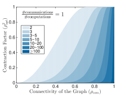
(a) [16], $A=W^{K}$

(b) Proposed scheme, $A=W^{K}$

(c) Proposed scheme, $A=P_{K}(W)$

Figure 1: Ratio between the number of communications and computations to achieve the centralized linear rate, as a function of the spectral gap $\rho_{\texttt{com}}$ and the gradient contraction factor $\rho_{\texttt{opt}}$. The proposed scheme employing multiple consensus rounds (subplot (b)) and Chebyshev acceleration (subplot (c)) is compared with [16] (subplot (a)).

In Fig. 1 we plot the minimum number $K$ of communication steps needed to achieve the rate of the centralized gradient as a function of $\rho_{\texttt{com}}$ and $\rho^{2}_{\texttt{opt}}$. Since only one computation is performed per iteration, this adjusts the ratio between the number of communications and computations. We compare our algorithm in the setting of Case 2 above, using $A=W^{K}$ or Chebyshev acceleration $A=P_{K}(W)$, with the distributed scheme in [16]. The figure shows that (i) Chebyshev acceleration helps to reduce the number of communications to sustain a given rate; and (ii) when $\rho_{\texttt{opt}}$ is close to $1$ ($\kappa$ is “large”), both instances of the proposed scheme need much less communication steps to attain the centralized rate than that in [16]. More specifically, to match the rate $\rho_{opt}$, one needs to run at least $K$ number of communications such that:

$$\rho_{com}^{K}=\begin{cases}\rho_{opt}^{2},&\text{[this work]};\\ \frac{\sqrt{1+\rho_{opt}}-\sqrt{1-\rho_{opt}}}{2},&\text{\cite[cite]{[\@@bibref{}{van2019distributed}{}{}]}}.\end{cases}$$

When $\rho_{opt}\rightarrow 0$, we have $({\sqrt{1+\rho_{opt}}-\sqrt{1-\rho_{opt}}})/{2}\approx{\rho_{opt}}/{2}$. Thus, $\rho_{opt}^{2}\leq{\rho_{opt}}/{2}$, since $\rho_{opt}\ll{1}/{2}$; hence, the scheme in [16] needs less number of communications than the proposed algorithm in the aforementioned setting. On the other hand, when $\rho_{opt}\rightarrow 1$, we have $({\sqrt{1+\rho_{opt}}-\sqrt{1-\rho_{opt}}})/{2}\approx{\rho_{opt}}/{\sqrt{2}}$. In this case, ${\rho_{opt}}/{\sqrt{2}}\leq{1}/{\sqrt{2}}\leq\rho_{opt}^{2}$; hence, our scheme require less communications than that in [16]. Moreover, since $({\sqrt{1+\rho_{opt}}-\sqrt{1-\rho_{opt}}})/{2}\leq{1}/{\sqrt{2}}<1$, when $\rho_{com}\rightarrow 1$, the scheme in [16] will need significantly more communication to match the centralized optimal rate.

VI Conclusion

We proposed a unified distributed algorithmic framework for composite optimization problems over networks; the algorithm includes many existing schemes as special cases. Linear rate was proved, leveraging a contraction operator-based anaysis. Under a proper choice of the design parameters, the rate dependency on the network and cost functions can be decoupled, which allowed us to determine the minimum number of communication steps needed to match the rate of centralized (proximal)-gradient methods.

Appendix A Convergence Analysis

We provide here a sketch of the proof of Theorem 3; see [17] for more details. Assumptions 2 and 3 are tacitly assumed hereafter.

Step 1: Auxiliary sequence and operator splitting: Lemma 5 below interpretes (4) as the fixed-point iterate of a suitably defined composition of contractive and nonexpansive operators.

Lemma 5 (​[17]).

Given the sequence $\{(Z^{k},X^{k},Y^{k})\}_{k}$ generated by Algorithm (4), define $U^{k}\triangleq[({Z}^{k})^{\top},({Y}^{k})^{\top}]^{\top}$. There holds

$$U^{k}=\begin{bmatrix}B&0\\ 0&B\sqrt{C}\end{bmatrix}\underset{\widetilde{U}^{k}}{\underbrace{\begin{bmatrix}\widetilde{Z}^{k}\\ \sqrt{C}\widetilde{Y}^{k}\end{bmatrix}}},\vspace{-0.2cm}$$

with $\{\widetilde{U}^{k}\}_{k}$ defined by the following dynamics

$$\widetilde{U}^{k+1}=\underbrace{\begin{bmatrix}(D-\gamma\nabla f)\circ\text{prox}_{\gamma g}\circ B&-\sqrt{C}\\ \sqrt{C}(D-\gamma\nabla f)\circ\text{prox}_{\gamma g}\circ B&I-C\end{bmatrix}}_{T}\widetilde{U}^{k},\quad k\geq 1,$$

and the initialization $\widetilde{Z}^{1}=\widetilde{Y}^{1}=(D-\gamma\nabla f)(X^{0})$. Furthermore, the operator $T$ can be decomposed as

$$T=\underbrace{\begin{bmatrix}I&-\sqrt{C}\\ \sqrt{C}&I-C\end{bmatrix}}_{\triangleq T_{C}}\underbrace{\begin{bmatrix}D-\gamma\nabla f&0\\ 0&I\end{bmatrix}}_{\triangleq T_{f}}\underbrace{\begin{bmatrix}\text{prox}_{\gamma g}&0\\ 0&I\end{bmatrix}}_{\triangleq T_{g}}\underbrace{\begin{bmatrix}B&0\\ 0&I\end{bmatrix}}_{\triangleq T_{B}},$$

where $T_{C}$ and $T_{B}$ are the operators associated with communications while $T_{f}$ and $T_{g}$ are the gradient and proximal operators, respectively. Finally, every fixed point $\widetilde{U}^{\star}\triangleq[\widetilde{Z}^{\star},\sqrt{C}\widetilde{Y}^{\star}]$ of $T$ is such that $B\widetilde{Z}^{\star}=1x^{\star\top}\in\mathcal{S}_{\texttt{Fix}}$.

Building on Lemma 5, the proof of Theorem 3 reduces to showing $\|\widetilde{Z}^{k}-\widetilde{Z}^{\star}\|=\mathcal{O}(\lambda^{k})$. To do so, Step 2 below studies the contraction (nonexpansive) properties of single operators composing $T$ while Step 3 chains these properties showing that $T$ is $\lambda$-contractive with respect to a suitable norm.

Step 2: On the properties of $T_{C}$, $T_{f}$, $T_{g}$ and $T_{B}$. We summarize next the main properties of the aforementioned operators; proofs of the results below can be found in [17]. We will use the following notation: given $X\in\mathbb{R}^{2m\times d}$, we denote by $(X)_{u}$ and $(X)_{\ell}$ its upper and lower $m\times d$ matrix-block.

Lemma 6.

The operator $T_{c}$ satisfies

$$\left\|T_{C}\,X-T_{C}\,Y\right\|^{2}_{\Lambda_{C}}=\left\|X-Y\right\|^{2}_{V_{C}},\quad\forall X,Y\in\mathbb{R}^{2m\times d},$$

where $\Lambda_{C}\triangleq\operatorname{\texttt{diag}}(I-C,I)$ and $V_{C}\triangleq\operatorname{\texttt{diag}}(I,I-C)$.

Lemma 7.

With $q$ defined in in Th. 3, $T_{f}$ satisfies: $\forall X,Y\in\mathbb{R}^{2m\times d}$,

$$\left\|(T_{f}\,X)_{u}-(T_{f}\,Y)_{u}\right\|^{2}\leq q^{2}\left\|(X)_{u}-(Y)_{u}\right\|^{2}\,\,\text{and}\,\,(T_{f}\,X)_{\ell}=(X)_{\ell}.$$

Lemma 8.

$T_{g}$ satisfies: $\forall X,Y\in\mathbb{R}^{2m\times d}$,

$$\left\|(T_{g}\,X)_{u}-(T_{g}\,Y)_{u}\right\|^{2}\leq\left\|(X)_{u}-(Y)_{u}\right\|^{2}\,\,\text{and}\,\,(T_{g}\,X)_{\ell}=(X)_{\ell}.$$

Lemma 9.

The operator $T_{B}$ satisfies:

$$\left\|(T_{B}\,X)_{u}\right\|^{2}=\left\|(X)_{u}\right\|_{B^{2}}^{2},\quad(T_{g}\,X)_{\ell}=(X)_{\ell},\quad\forall X\in\mathbb{R}^{2m\times d}.$$

Step 3: Chaining Lemmata 6-9. Define the matrices $Q_{f}\triangleq\operatorname{\texttt{diag}}(q^{2}I,\,I)$ and $\Lambda_{B}=\operatorname{\texttt{diag}}(B^{2},I);$ the contraction property of $T$ are implied by the following chain: $\forall\,X,Y\in\mathbb{R}^{2m\times d}$ with $X_{\ell},Y_{\ell}\in{\texttt{span}}(\sqrt{C})$,

$$\left\|T\,X-T\,Y\right\|_{\Lambda_{C}}^{2}\stackrel{{\scriptstyle Lm.~{}\ref{lem:contraction_T_c}}}{{=}}\left\|T_{f}\circ T_{g}\circ T_{B}\,(X-Y)\right\|_{V_{C}}^{2}$$

$$\stackrel{{\scriptstyle Lm.~{}\ref{lem:contraction_T_f}}}{{\leq}}\left\|T_{g}\circ T_{B}\,(X-Y)\right\|_{V_{C}Q_{f}}^{2}\stackrel{{\scriptstyle Lm.~{}\ref{lem:contraction_T_g}}}{{\leq}}\left\|T_{B}\,(X-Y)\right\|_{V_{C}Q_{f}}^{2}$$

$$\stackrel{{\scriptstyle Lm.~{}\ref{lem:contraction_T_B}}}{{=}}\left\|X-Y\right\|_{V_{C}Q_{f}\Lambda_{B}}^{2}\stackrel{{\scriptstyle(*)}}{{\leq}}\lambda\,\left\|X-Y\right\|_{\Lambda_{C}}^{2},$$

where $V_{C}Q_{f}\Lambda_{B}=\operatorname{\texttt{diag}}(q^{2}B^{2},I-C)$, $\lambda$ is defined in (7); and (*) is due to the following two facts: i) $q^{2}\|(Z)_{u}\|^{2}_{B^{2}}=q^{2}\|(I-C)^{\frac{1}{2}}(Z)_{u}\|^{2}_{B^{2}(I-C)^{-1}}\leq q^{2}\lambda_{\text{max}}(B^{2}(I-C)^{-1})\|(I-C)^{\frac{1}{2}}(Z)_{u}\|^{2}=q^{2}\lambda_{\text{max}}(B^{2}(I-C)^{-1})\left\|(Z)_{u}\right\|^{2}_{I-C},$ for all $\,(Z)_{u}\in\mathbb{R}^{m\times d}$; and ii) $X_{\ell},Y_{\ell}\in{\texttt{span}}(\sqrt{C})$.

References

- [1] W. Shi, Q. Ling, G. Wu, and W. Yin, “EXTRA: An exact first-order algorithm for decentralized consensus optimization,” SIAM Journal on Optimization, vol. 25, no. 2, pp. 944–966, 2015.
- [2] J. Xu, S. Zhu, Y. C. Soh, and L. Xie, “Augmented distributed gradient methods for multi-agent optimization under uncoordinated constant stepsizes,” in Proceedings of 54th IEEE Conference on Decision and Control (CDC), 2015, pp. 2055–2060.
- [3] P. Di Lorenzo and G. Scutari, “Next: In-network nonconvex optimization,” IEEE Transactions on Signal and Information Processing over Networks, vol. 2, no. 2, pp. 120–136, 2016.
- [4] G. Scutari and Y. Sun, “Distributed nonconvex constrained optimization over time-varying digraphs,” Mathematical Programming, vol. 176, no. 1–2, pp. 497–544, July 2019.
- [5] Y. Sun, A. Daneshmand, and G. Scutari, “Convergence rate of distributed optimization algorithms based on gradient tracking,” arXiv:1905.02637, 2019.
- [6] A. Nedich, A. Olshevsky, and W. Shi, “Achieving geometric convergence for distributed optimization over time-varying graphs,” SIAM J. on Optimization, vol. 27, no. 4, pp. 2597–2633, 2017.
- [7] Z. Li, W. Shi, and M. Yan, “A decentralized proximal-gradient method with network independent step-sizes and separated convergence rates,” IEEE Transactions on Signal Processing, vol. 67, no. 17, pp. 4494–4506, 2019.
- [8] K. Yuan, B. Ying, X. Zhao, and A. H. Sayed, “Exact diffusion for distributed optimization and learning?part i: Algorithm development,” IEEE Transactions on Signal Processing, vol. 67, no. 3, pp. 708–723, 2018.
- [9] K. Scaman, F. Bach, S. Bubeck, Y. T. Lee, and L. Massoulié, “Optimal algorithms for smooth and strongly convex distributed optimization in networks,” in Proceedings of the 34th International Conference on Machine Learning, 2017, pp. 3027–3036.
- [10] G. Qu and N. Li, “Harnessing smoothness to accelerate distributed optimization,” IEEE Transactions on Control of Network Systems, vol. 5, no. 3, pp. 1245–1260, 2017.
- [11] D. Jakovetić, “A unification and generalization of exact distributed first-order methods,” IEEE Transactions on Signal and Information Processing over Networks, vol. 5, no. 1, pp. 31–46, 2018.
- [12] F. Mansoori and E. Wei, “A general framework of exact primal-dual first order algorithms for distributed optimization,” arXiv preprint arXiv:1903.12601, 2019.
- [13] S. A. Alghunaim, K. Yuan, and A. H. Sayed, “A linearly convergent proximal gradient algorithm for decentralized optimization,” arXiv preprint arXiv:1905.07996, 2019.
- [14] A. Sundararajan, B. V. Scoy, and L. Lessard, “A canonical form for first-order distributed optimization algorithms,” arXiv:1809.08709, 2018.
- [15] A. Sundararajan, B. Hu, and L. Lessard, “Robust convergence analysis of distributed optimization algorithms,” in Proc. of the 55th Annual Allerton Conference on Communication, Control, and Computing (Allerton).
- [16] B. Van Scoy and L. Lessard, “Distributed optimization of nonconvex functions over time-varying graphs,” arXiv preprint arXiv:1905.11982, 2019.
- [17] J. Xu, Y. Sun, Y. Tian, and G. Scutari, “A unified algorithmic framework for distributed composite optimization,” Purdue Technical Report, July 2019. [Online]. Available: arxiv preprint
- [18] A. Wien, Iterative solution of large linear systems. Lecture Notes, TU Wien, 2011.