4011

SCHWABE, GLEISSBERG, SUESS-DE VRIES: TOWARDS A CONSISTENT MODEL OF PLANETARY SYNCHRONIZATION OF SOLAR CYCLES

Abstract: Aiming at a consistent planetary synchronization model of both short-term and long-term solar cycles, we start with an analysis of Schove’s historical data of cycle maxima. Their deviations (residuals) from the average cycle duration of 11.07 years show a high degree of regularity, comprising a dominant 200-year period (Suess-de Vries cycle), and a few periods around 100 years (Gleissberg cycle). Encouraged by their robustness, we support previous forecasts of an upcoming grand minimum in the 21st century. To explain the long-term cycles, we enhance our tidally synchronized solar dynamo model by a modulation of the field storage capacity of the tachocline with the orbital angular momentum of the Sun, which is dominated by the 19.86-year periodicity of the Jupiter-Saturn synodes. This modulation of the 22.14 years Hale cycle leads to a 193-year beat period of dynamo activity which is indeed close to the Suess-de Vries cycle. For stronger dynamo modulation, the model produces additional peaks at typical Gleissberg frequencies, which seem to be explainable by the non-linearities of the basic beat process, leading to a bi-modality of the Schwabe cycle. However, a complementary role of beat periods between the Schwabe cycle and the Jupiter-Uranus/Neptune synodic cycles cannot be completely excluded.

1 Introduction

Solar activity is governed by the 11-year Schwabe cycle (or 22-year Hale cycle), and a few long-term cycles superposed on it [1, 2]. Among those, the Gleissberg cycle (90 years) and the Suess-de Vries cycle (200 years) figure most prominently, while the Hallstatt cycle (2300 years) may play a “super-modulating” role [3]. Recent solar dynamo models have been successful in understanding both the typical time scale of the Schwabe cycle as well as the shape of the butterfly diagram of sunspots. In the framework of non-linear dynamo models, the disparity between short- and long-term cycles was explained as a consequence of the small magnetic Prandtl number in the tachocline region [4].

This being said, some features of the solar cycles leave us with the nagging feeling that conventional dynamo models might not be the end of the story. As a case in point, Dicke’s ratio [5] of the mean square of the residuals (i.e. the distances between the actual minima and the hypothetical minima of a perfect 11.07-year cycle) to the mean square of the differences between two consecutive residuals, points decisively to a clocked process, in stark contrast to a random walk process [6]. As for the long-term cycles, it is foremost the sharpness of the 200-year Suess-de Vries cycle which leaves us unconvinced about the skill of present dynamo models for explaining it. Even if one denies Dicke’s question “Is there chronometer hidden deep in the Sun?” [5], it is the counter-question concerning a possible external clock for the solar dynamo which leads us, rather inevitably, into the field of planetary synchronization.

Despite the long history of planetary synchronization models, going back to early speculations of Wolf [7], there has always been some air of “astrology” hanging about them. Distinguishing between models based on tidal forcing and models based on spin-orbit coupling, there is indeed good reason for profound skepticism towards both of them. Tidal forcing models can easily be ridiculed by the tiny acceleration of $\sim 10^{-10}$ ms^-2 as exerted by planets [8], leading to a negligible tidal height of not more than 1 mm. Spin-orbit models [9, 10] have likewise been criticized [11] for not being able to conclusively explain how any internal differential motion could be produced from the free-fall motion of the Sun around the solar system’s barycenter (SSB), however impressive the amplitude of that motion (around 1 solar diameter) and its speed (until 15 m/s) may ever appear.

Even if recognizing the seriousness of such objections, some more specific considerations seem appropriate. As for the tidal force, one should note that the typical tidal height, as produced by a planet of mass $m$ at distance $d$ from the Sun, $h_{\rm tidal}=GmR^{2}_{\rm tacho}/(g_{\rm tacho}d^{3})=O(1$ mm) translates - via virial theorem - into a non-negligible velocity of $v\sim(2g_{\rm tacho}h_{\rm tidal})^{1/2}\approx 1$ m/s, when employing the huge gravity at the tachocline of $g_{\rm tacho}\approx 500$ m/s². Likewise, for the spin-orbit model it has been argued [12, 13] that some 0.1 per cent of the typical orbital angular momentum variation of the Sun ($5\times 10^{40}$ Nms) might well be transferred into internal differential motion, which would amount to a velocity scale of 4 m/s when applied only to the 2 per cent of the total solar mass as concentrated in the convection zone. Again, velocities of that scale could definitely be dynamo relevant, remembering a similar scale of 10 m/s for the meridional circulation [1]. Partially related to the distinction between tidal versus spin-orbit models, planetary forcing models can further be classified into models of hard synchronization of the basic Schwabe cycle (for example, with the 11.07 years spring tide period of the tidally dominant Venus-Earth-Jupiter system [6, 14, 15, 16, 17, 18]) and models of soft modulations of this Schwabe cycle, with main focus on the Gleissberg, Suess-de Vries and Hallstatt cycle [19, 20, 21, 22, 24, 25, 26, 27, 28].

Instead of linking the periods of Sun’s long-term cycles to corresponding periods of planetary influences, we pursue here another concept, in which long-term cycles emerge as beat periods between the basic Hale/Schwabe cycle with the typical synodic periods of Jupiter with other Jovian planets. The beat period of 193 years, as resulting from the 22.14-year Hale cycle and the 19.86-year synodic cycle of Jupiter and Saturn, has been noticed by several authors [15, 29]. Likewise, one may wonder if the beat periods 55.8 years and 82.7 years, arising between the 11.07 Schwabe cycle and the Jupiter-Uranus synode (13.81 years) and the Jupiter-Neptune synode (12.78 years), respectively, could somehow be related to the Gleissberg cycle.

The aim of this paper is to corroborate how such beat periods actually emerge in our specific solar dynamo model [6], which had already demonstrated synchronization of the Schwabe cycle with the 11.07 years tidal period, based on the resonance of the intrinsic helicity oscillations of the current-driven $m=1$ Tayler instability with the $m=2$ tidal forcing [30, 31]. Before entering this topic, we reconstruct the typical Gleissberg and Suess-de Vries periods from the long series of solar cycle maxima data as bequeathed to us by Schove [32, 33, 34]. The paper will close with a summary and a short discussion of open issues.

2 Spectral analyses of cycle maxima

In a meticulous effort over three decades [32, 33, 34], Schove had tried to identify the minima and maxima of the solar cycle for nearly two and a half millennia, relying strongly on historical aurora borealis observations. Although Schove’s time series are considered by some researchers as “archaic” [35], they are still hard to replace when it comes to the very dating of individual maxima and minima for early times (hopefully, a careful analysis of existing ¹⁴C or ¹⁰Be data, e.g. [36], may once allow to verify, or falsify, Schove’s time series, at least for A.D. 1400 onward). Based on Schove’s minima data, in [6] we had computed Dicke’s ratio [5] to argue in favour of the solar cycle as being a clocked, rather than a random walk process. In Fig. 1a we show now the sequence of maxima data after having subtracted two different linear functions with an 11.07-year and an 11.11-year trend, respectively. Obviously, the residuals from the 11.07-year trend form a rather horizontal band, while the residuals from the 11.11-year trend still exhibit an unresolved downward inclination. This slight, but important, difference disproves the often heard objection against Schove’s data (e.g. [35], taking a loose remark on page 131 of [32] too literally) as being biased by a strict constraint of “9 maxima in 100 years”. The fact that the 11.07-year trend appears naturally from Schove’s data, without ever being enforced by him, speaks strongly in favour of the validity of that cycle period. Another interesting feature is the bi-modality of the histogram of the cycle durations (Fig. 1 c), with two maxima at around 10 and 12 years flanking the so-called Wilson gap [2], which will play an important role in our further analysis.

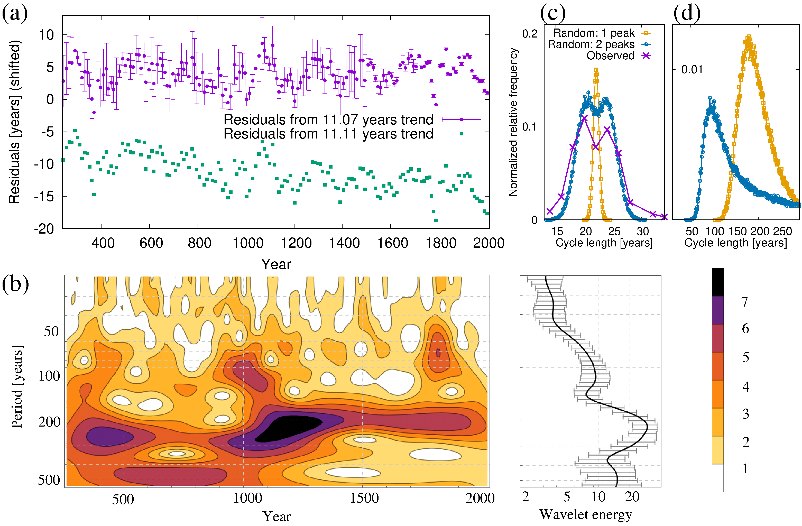
Figure 1: (a) Residuals of the cycle maxima [34] from two trends with 11.07-year (including error bars) and 11.11-year period (differently shifted). (b) Wavelet analysis of the data of (a). Error bars of the wavelet energy indicate 95 per cent two-sided confidence intervals. (c) Purple - Histogram of the (doubled) cycle lengths according to (a). Orange - Histogram (reduced by factor 5) of 10⁵ random numbers $T_{\rm ran}$ centered narrowly around 22.14 years. Blue - Histogram of 10⁵ random numbers $T_{\rm ran}$ bi-modally centered around 19.86 and 24.42 years (similar as observed data). (d) Histogram of arising beat periods $19.86\;T_{\rm ran}/|T_{\rm ran}-19.86|$ using the random numbers $T_{\rm ran}$ from (c). While the narrowly centered $T_{\rm ran}$ (orange) produce a dominant beat period around 180 years, the bi-modally centered $T_{\rm ran}$ (blue) produce a beat period around 90 years.

While long-term solar cycles are usually inferred from various continuous data sets (e.g., ¹⁰Be or ¹⁴C isotopes [26, 42] or paleoclimate data [37]), quite similar cycle periods can also be identified by analyzing the time series of the residuals of the cycle maxima or minima. The “(O-C) residuals”, as computed in [38] for data between A.D. 1610 - 1996, have revealed peaks at a Suess-de Vries period of 188 years, a Gleissberg cycle of 87 years, and an additional (unnamed) 40 years cycle. Here, we take advantage of Schove’s much longer data-set of cycle maxima, complemented by Hathaway’s data [2] for the later years of the total interval A.D. 242 - 2000. The starting year A.D. 242 has been chosen since the value before that date is the first one that is missing in [34]. For frequency analysis, we utilize first a wavelet transform (Fig. 1b, using the Morlet wavelet with resolution parameter $2\pi$ and a gaped wavelet algorithm for solving the edge problem), and additionally a generalized Lomb-Scargle method (Fig. 2) which accounts for different prior uncertainties for individual data points. Specifically, our data and their uncertainties are compiled as follows: for the early years A.D. 241 - 1493 they are taken from Appendix B of Schove’s most recent and comprehensive publication [34]. As uncertainties, we use the comparably large values from the older publication [32]. Between A.D. 1506 - 1700, we use the maxima data and their uncertainties from Table 2 of [34]. From A.D. 1718 onward, we opted for a somewhat optimistic uncertainty of 0.25 years, not least in order to give those recent data a higher statistical weight compared to the older ones. The data from A.D. 1718 - 1761 are taken again from [34], whilst all subsequent maxima are taken from the more modern table of [2] (they mainly coincide with the data of [34]).

Figure 2: (a) Lomb-Scargle periodogram for the maxima residuals, when taking into account data (and their uncertainties) from five different time intervals. The dashed horizontal line in each sub-panel indicates a 25 per cent false alarm probability. (b) Complete picture and two zooms of the residuals, showing also five different approximations with those harmonics that are statistically significant for the respective fitting intervals, as indicated by full circles in (a). Cycles longer (shorter) than 11.07 years correspond to a positve (negative) slope of the curves.

With view on the decreasing reliableness of Schove’s data before A.D. 1600, say, we compute the generalized Lomb-Scargle periodograms (Fig. 2a) for different underlying time intervals. Apart from a general broadening of the peaks (and some minor shifts), when going over to shorter (i.e., later) time intervals, we observe quite robust features such as a dominant Suess-de Vries cycle around 200 years (which also dominates the wavelet spectrum, see Fig. 1b) and one or a few Gleissberg-type cycles around 100 years, in good agreement with [29, 38]. The generalized Lomb-Scargle method provides us also with a significance level (here: 25 per cent false alarm probability, indicated by the dashed lines in Fig. 2a) to identify the most significant peaks for each underlying time interval. The various data reconstructions with the corresponding sets of significant harmonics (as indicated by the full circles in Fig. 2a) are shown in Fig. 2b. Interestingly, the extrapolations of the various fit curves show a rather consistent tendency towards longer solar cycles throughout the 21st century. With regard to the inverse relationship between the cycle length and the amplitude of the (following) cycle [2], we support the forecasts of a new grand minimum that were already made by various authors [22, 29, 38].

3 A synchronized and modulated dynamo model

We have seen that the period of the dominant Suess-de Vries cycle as inferred from Schove’s maxima data is very close to 200 years, which is highly consistent with previous results based on ¹⁰Be and ¹⁴C data [42], and various climate related data [37]. The robustness and relative sharpness of that peak suggests a link to planetary forcings with equal or similar periods, as discussed by many authors [19, 20, 21, 22, 24, 25, 26, 27, 28]. Another explanation, which also brings us close to the 200 years cycle, relies on the beat period of 193 years [15, 29] that arises from the interplay of the 22.14-year Hale cycle and the 19.86-year synodic cycle of Jupiter and Saturn (which produces, according to Fig. 3, the dominant component of the solar motion around the SSB). A similar beat mechanism between the 11.07-year Schwabe cycle and the 13.81-year Jupiter-Uranus and/or the 12.78-year Jupiter-Neptune synode may likewise be considered a candidate for producing Gleissberg-type periods of 55.8 years and 82.7 years, respectively.

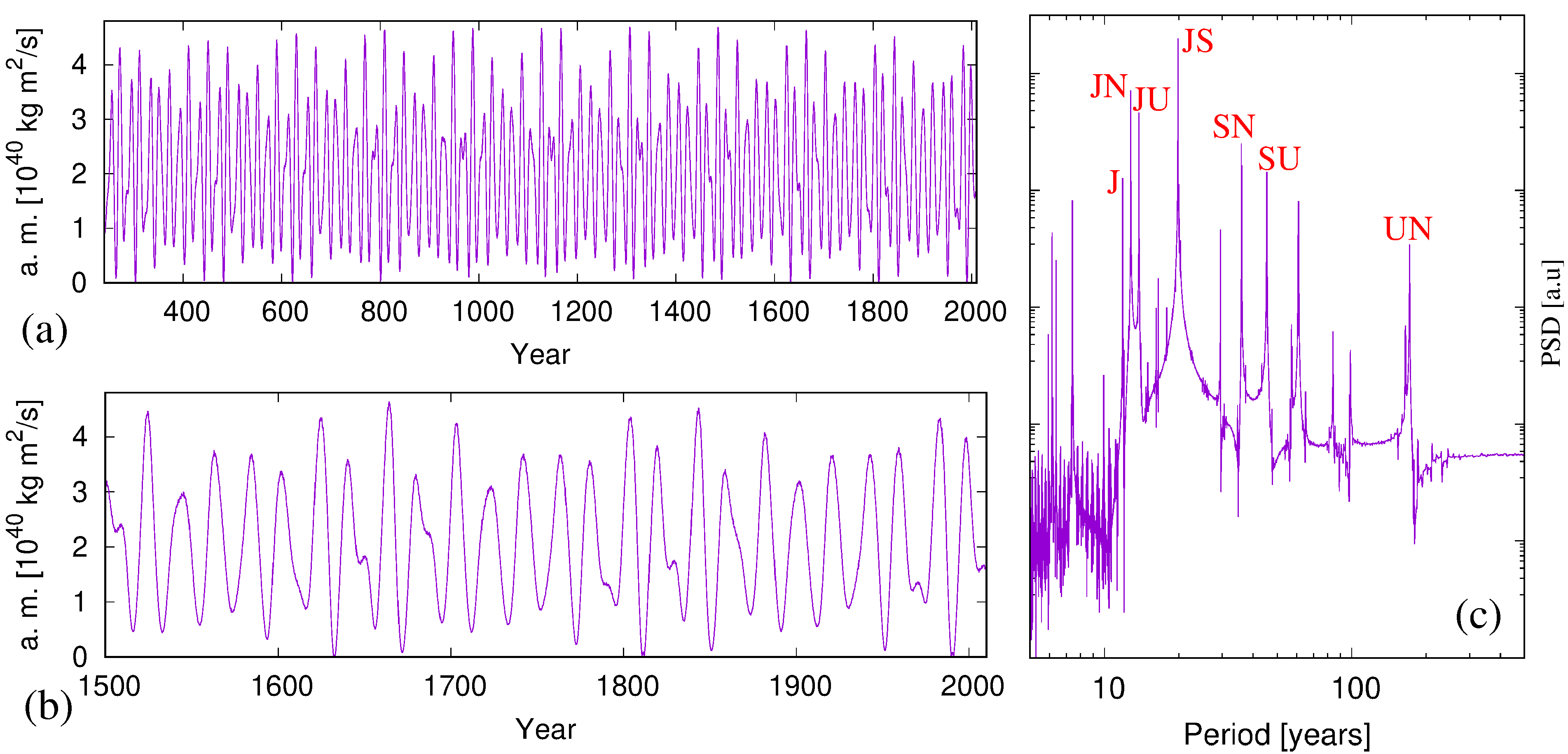
Figure 3: (a) Time series of the orbital angular momentum (a.m.) of the Sun around the SSB in the interval A.D. 240-2001, and (b) zoom thereof for A.D. 1500-2001, based on the DE431 ephemerides [39]. (c) PSD of the angular momentum for the long interval 13199 B.C.-A.D. 17000, with some individual peaks attributed to planetary synodes (cf. [28]): JN: Jupiter-Neptune (12.78 years), JU: Jupiter-Uranus (13.95 years), JS: Jupiter-Saturn (19.86 years), SN: Saturn-Neptune (35.87 years), SU: Saturn-Uranus (45.36 years), UN: Uranus-Neptune (171.39 years). J indicates the 11.86 years period of Jupiter.

To corroborate this idea, we extend the dynamo model of [6], in which the Hale cycle was produced by synchronizing a conventional $\alpha-\Omega$ dynamo with an additional 11.07-year oscillation of the $\alpha$ effect. This oscillation of $\alpha$ (related to the helicity of the $m=1$ Tayler instability or, alternatively, an $m=1$ magneto-Rossby wave [40, 41]) was, in turn, assumed to be resonantly excited by an $m=2$ planetary tidal forcing. As in [6], we use the equation system

$$\frac{{\partial}B(\theta,t)}{{\partial}t} = \omega(\theta,t)\frac{\partial A(\theta,t)}{\partial\theta}+\frac{\partial^{2}B(\theta,t)}{\partial\theta^{2}}-\kappa(t)B^{3}(\theta,t),$$ (1)

$$\frac{{\partial}A(\theta,t)}{{\partial}t} = \alpha(\theta,t)B(\theta,t)+\frac{\partial^{2}A(\theta,t)}{\partial\theta^{2}}$$ (2)

for the vector potential $A(\theta,t)$ of the poloidal field at co-latitude $\theta$ and time $t$, and the toroidal field $B(\theta,t)$.

According to [1] we employ a $\theta$-dependence of the $\omega$-effect in the form

$$\omega(\theta) = \omega_{0}(1-0.939-0.136\cos^{2}(\theta)-0.1457\cos^{4}(\theta))\sin(\theta)$$

with a plausible value $\omega_{0}=10000$. The helical source term $\alpha$ comprises, first, a non-periodic part

$$\alpha^{c}(\theta,t) = \alpha^{c}_{0}(1+\xi(t))\sin(2\theta)/{(1+q^{c}_{\alpha}B^{2}(\theta,t))},$$

with a constant $\alpha^{c}_{0}$ and a noise term $\xi(t)$, and second, a periodic part

$$\alpha^{p}(\theta,t) = \alpha^{p}_{0}\sin(2\pi t/11.07)B^{2}(\theta,t)/(1+q^{p}_{\alpha}B^{4}(\theta,t))S(\theta),$$

where $S(\theta)$ is a hemispherically asymmetric (and slightly smoothed) term that is non-zero only for $55^{\circ}<\theta<125^{\circ}$. The noise $\xi(t)$, defined by the correlator

$$\langle\xi(t)\xi(t+t_{1})\rangle=D^{2}(1-|t_{1}|/t_{\rm corr})\Theta(1-|t_{1}|/t_{\rm corr}),$$

is numerically realized by random numbers with variance $D^{2}$ which are held constant over a correlation time $t_{\rm corr}$. For more details of the numerical model, see [6].

The term $\kappa(t)B^{3}(\theta,t)$ had been included to account for losses owing to magnetic buoyancy. While we openly admit that the necessary spin-orbit type coupling mechanism of the orbital angular momentum of the Sun around the SSB into some dynamo relevant parameters remains an open question (for ideas, see [9, 12, 13, 23]) we employ in the following a modulation of the parameter $\kappa$ with the time series of the angular momentum. Since $\kappa$ is related to the adiabaticity in the tachocline which is, in turn, a very sensitive parameter [25], its modification by some sort of spin-orbit coupling seems, at least, not completely unrealistic.

What is now the effect of this modulation of $\kappa$ on the dynamo process? Figure 4 illustrates paradigmatic solutions of Eqs. (1-2) with increasing complexity. First, Fig. 4a shows a conventional $\alpha-\Omega$ dynamo, without any synchronization, i.e., with $\alpha^{p}_{0}=0$. This specific dynamo happens to produce a quadrupole field with an oscillation period of 24.39 years which is close, but not identical, to the Hale cycle (see the PSD in Fig. 4f). When adding to this dynamo an oscillatory $\alpha$-term with $\alpha^{p}_{0}=50$, we obtain the clear dipole configuration of Fig. 4b, synchronized now to the precise Hale period of 22.14 years.

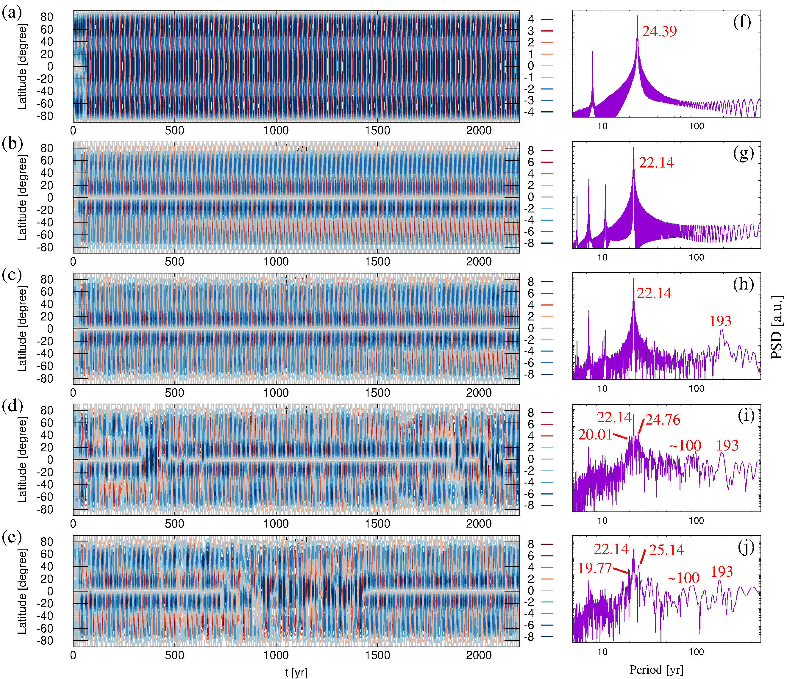
Figure 4: (a-e) Behaviour of $B(\theta,t)$, and (f-j) PSD for $B(72^{\circ},t)$, with the common parameters $\omega_{0}=10000$, $\alpha^{c}_{0}=15$, $q^{p}_{\alpha}=0.2$, $q^{c}_{\alpha}=0.8$. The remaining parameters vary. (a,f) $\alpha^{p}_{0}=0$, $\kappa=0.5$, $D=0$: a classical $\alpha-\Omega$ dynamo producing a quadrupole with 24.39-year period. (b,g) $\alpha^{p}_{0}=50$, $\kappa=0.75$, $D=0$: a tidally synchronized dynamo producing a dipole with 22.14-year period. (c,h) $\alpha^{p}_{0}=50$, $\kappa(t)=0.5+0.5m(t)$, $D=0.2$: as (b,g), but with noise and a modulation of $\kappa$ with an angular momentum function $m(t)$ according to Fig. 3(a) (the maximum being normalized to 1). As seen in (h), this dipole solution contains a beat period of 193 years. (d,i) $\alpha^{p}_{0}=50$, $\kappa(t)=0.18+1.0m(t)$, $D=0.215$: similar to (c,h), but with stronger $\kappa$ variation. (i) shows some peaks around 100 years, reminiscent of the Gleissberg cycle(s). (e,j) $\alpha^{p}_{0}=50$, $\kappa(t)=0.17+1.3m_{\rm JS}(t)$, $D=0.23$; similar to (d,i), but with a simpler angular momentum $m_{\rm JS}(t)$ which is restricted to the 19.86-years periodic part resulting from Jupiter and Saturn only.

In the next step, see Fig. 4c, we assume a modulation of the parameter $\kappa$ with the angular momentum time series from Fig. 3 (plus some weak noise with $D=0.2$). Thereby, we obtain a clear additional peak (Fig. 4h) at the 193-year beat period between the underlying 22.14-year Hale cycle and the dominating (Jupiter-Saturn related) 19.86-year period of the modulation of $\kappa$. Interestingly, this 193-year signal is connected with the same type of variation of the “magnetic equator” as observed in [43] (although with a Gleissberg-type period in their case).

Figure 4d shows a similar dynamo run, this time with a stronger variation of $\kappa$, which obviously leads to some intervening quadrupolar fields during the run. The corresponding PSD (Fig. 4i) exhibits now also some Gleissberg-type peaks around 100 years. In parallel with that, the basic Hale cycle develops two side peaks at around 20.0 years and 24.8 years, not dissimilar to the observed ones in Fig. 1c. Apparently, the dynamo undergoes an intermediate locking close to the 19.86 years modulation cycle which, in turn, must be compensated by some longer cycles. It is these prolonged Hale cycles which produce the shortened Gleissberg-type beat periods around 100 years (see also Fig. 1c,d for plausibilization).

To clarify whether such Gleissberg-type peaks may alternatively emerge as beat periods between the Schwabe cycle and the 13.81-year Jupiter-Uranus and/or the 12.78-year Jupiter-Neptune synode, we employ a simplified angular momentum time series where only the influence of Jupiter and Saturn is taken into account, whereas the frequencies due to other planets are omitted. The resulting PSD (Fig. 4j) continues to show some Gleissberg-type peaks, which - together with the sustained two side bands of the Hale cycle - speaks in favour of their non-linear origin discussed above. Yet, the also observable reduction of the ”noisiness” of the PSD (Fig. 4j compared with Fig. 4i) suggests at least some complementary role of the other frequencies which are present in the Sun’s movement around the SSB.

4 Conclusions

The Lomb-Scargle and wavelet analyses of Schove’s solar cycle maxima data have reconfirmed a Schwabe cycle with 11.07-year period, superposed by a clear Suess-de Vries cycle with a period of appr. 200 years, and one or a few Gleissberg-type cycles around 100-year periodicity. An extrapolation of the dominant harmonics points robustly to a next grand minimum in the 21st century, in accordance with previous predictions. The related decrease of solar activity may allow for a better differential diagnostics of the respective weights of the two key climate drivers, solar activity/irradiance and anthropogenic greenhouse gases, whose individual effects were hard to disentangle in the course of their widely parallel rise during the last century.

Our tidally synchronized solar dynamo model, enhanced by a (yet poorly understood) spin-orbit coupling effect based on the dominant 19.86 years period of Jupiter-Saturn synodes, has lead to a clear spectral peak at the beat period of 193 years, which is close to the observed Suess-de Vries cycle. The robustness of this cycle, in turn, lends also greater plausibility to the clocked character of the underlying 22.14 Hale cycle (a simple random-walk process with average 22.14-years periodicity, but large phase-shifts, would hardly show such a beat period). Furthermore, for sufficiently strong modulation we observe two side-bands of the Hale cycle, one centered around the 19.86-year Jupiter-Saturn period, the other one around 24.5 years (to compensate for the “too short” cycles, when keeping pace with the basic 11.07 years tidal forcing). It appears that those prolonged Hale cycles can produce new Gleissberg-like beat periods around 100 years. However, a complementary explanation in terms of beat periods between the Schwabe cycle and the Jupiter-Uranus/Neptune synodes cannot be completely excluded.

What we have not aimed at in this paper is any prediction of the very timing of grand minima. This would require a good understanding of the phase relation between the two basic physical mechanisms underlying this work: tidal synchronization of helicity oscillations, and coupling of the Sun’s orbital motion around the SSB to internal motion. It also remains to be seen whether or not the Hallstatt cycle could be incorporated into the concept. The consistent reproduction of the Schwabe cycle, its two side-bands (flanking the Wilson gap), the Suess-de Vries and some Gleissberg-type cycles, as accomplished in this paper, might be a promising starting point for further investigations.

References

- [1] P. Charbonneau Dynamo models of the solar cycle. Living Rev. Sol. Phys. , vol. 7 (2010), p. 3.
- [2] D.H. Hathaway The solar cycle. Liv. Rev. Sol. Phys., vol. 7 (2010), Art.No. 1
- [3] J. Beer, S.M. Tobias, N.O. Weiss On long-term modulation of the Sun’s magnetic cycle.. Mon. Not. R. Astron. Soc., vol. 473 (2018), p. 1596.
- [4] S.M. Tobias Grand minima in nonlinear dynamos. Astron. Astrophys., vol. 307 (1996), p. L21.
- [5] R.H. Dicke Is there a chronometer hidden deep in the sun? Nature, vol. 276 (1996), p. 676.
- [6] F. Stefani, A. Giesecke, T. Weier A model of a tidally synchronized solar dynamo. Solar Phys., vol. 294 (2019), p. 60.
- [7] R. Wolf Extract of a letter to Mr. Carrington. Mon. Not. R. Astron. Soc., vol. 19 (1859), p. 85.
- [8] D.K. Callebaut, C. de Jager, S, Duhau The influence of planetary attractions on the solar tachocline. J. Atmos. Sol.-Terr. Phys., vol. 80 (2012), p. 73.
- [9] T.V. Zaqarashvili On a possible generation mechanism for the solar cycle. Astrophys. J., vol. 487 (1997), p. 930.
- [10] D.A. Jucket Solar activity cycles, north/south asymmetries, and differential rotation associated with solar spin-orbit variations. Solar Phys., vol. 191 (2000), p. 201.
- [11] J.H. Shirley Axial rotation, orbital revolution and solar spin-orbit coupling. Mon. Not. R. Astron. Soc., vol. 368 (2006), p. 280.
- [12] I.R.G. Wilson Does a spin-orbit coupling between the Sun and the Jovian planets govern the solar cycle? Publ. Astron. Soc. Austr., vol. 25 (2008), p. 85.
- [13] G. Sharp Are Uranus and Neptune responsible for solar grand minima and solar cycle modulation? Int J. Astron. Astrophys., vol. 3 (2013), p. 260.
- [14] C.C. Hung Apparent relations between solar activity and solar tides caused by the planets. NASA/TM-2007-214817 (2007).
- [15] I.R.G. Wilson The Venus-Earth-Jupiter spin-orbit coupling model. Pattern Recogn. Phys., vol. 1 (2013), p. 147.
- [16] V.P. Okhlopkov The 11-year cycle of solar activity and configurations of the planets. Mosc. U. Phys. Bull., vol. 69 (2014), p. 257.
- [17] F. Stefani, A. Giesecke, N. Weber, T. Weier. Synchronized helicity oscillations: a link between planetary tides and the solar cycle? Solar Phys., vol. 291 (2016), p. 2197.
- [18] F. Stefani, A. Giesecke, N. Weber, T. Weier. On the synchronizability of Tayler-Spruit and Babcock-Leighton type dynamos. Solar Phys., vol. 293 (2018), p. 12.
- [19] P.D. Jose Sun’s motion and sunspots. Astron. J., vol. 70 (1965), p. 193.
- [20] R.W. Fairbridge, J.H. Shirley Prolonged minima and the 179-yr cycle of the solar inertial motions. Solar Phys., vol. 110 (1987), p. 191.
- [21] I. Charvatova Solar-terrestrial and climatic phenomena in relation to solar inertial motion. Surv. Geophys., vol. 18 (1997), p. 131.
- [22] T. Landscheidt Extrema in sunspot cycle linked to Sun’s motion. Solar Phys., vol. 189 (1999), p. 413.
- [23] M. Palus, J. Kurths, U. Schwarz, D. Novotna, I. Charvatova Is the solar activity cycle synchronized with the solar inertial motion? Int. J. Bifurc. Chaos Appl. Sci. Eng., vol. 10 (2000), p. 2519.
- [24] C.L. Wolff, P.N. Patrone A new way that planets can effect the sun. Solar Phys., vol. 266 (2010), p. 227.
- [25] J.A. Abreu, J. Beer, A. Ferriz-Mas, K.G. McCracken, F. Steinhilber Is there a planetary influence on solar activity? Astron. Astrophys., vol. 548 (2012), p. A88.
- [26] K.G. McCracken, J. Beer, F. Steinhilber Evidence for planetary forcing of the cosmic ray intensity and solar activity throughout the past 9400 years. Solar Phys., vol. 289 (2014), p. 3207.
- [27] R.G. Cionco, W. Soon A phenomenological study of the timing of solar activity minima of the last millennium through a physical modeling of the sun-planets interaction New Astron., vol. 34 (2015), p. 164.
- [28] N. Scafetta, F Milani, A. Bianchini, S. Ortolani On the astronomical origin of the Hallstatt oscillation found in radiocarbon and climate records throughout the Holocene. Earth Sci. Rev., vol. 162 (2016), p. 24.
- [29] J.-E. Solheim The sunspot cycle length modulated by planets? Pattern Recogn. Phys., vol. 1 (2013), p. 159.
- [30] N. Weber, V. Galindo, F. Stefani, T Weier. The Tayler instability at low magnetic Prandtl numbers: between chiral symmetry breaking and helicity oscillations. New J. Phys., vol. 15 (2012), Art. No. 113013.
- [31] R. Stepanov, F. Stefani Electromagnetic forcing of a flow with the azimuthal wave number m=2 in cylindrical geometry. Magnetohydrodynamics, vol. 55 (2019), p. 207.
- [32] D.J. Schove The sunspot cycle, 649 B.C. to A.D. 2000. J. Geophys. Res., vol. 60 (1955), p. 127.
- [33] D.J. Schove Sunspot turning-points and aurorae since A.D. 1510. Solar Phys., vol. 63 (1979), p. 423.
- [34] D.J. Schove Sunspot cycles. Hutchinson Ross Publishing Company (1983), Stroudsburg, Pennsylvania.
- [35] I.G. Usoskin A history of solar activity over millennia. Liv. Rev. Sol. Phys., vol. 14 (2017), p. 3.
- [36] A.-M. Berggren et al. A 600-year annual 10Be record from the NGRIP ice core, Greenland. Geophys. Res. Lett., vol. 36 (2009), p. L11801.
- [37] H.-J. Lüdecke, C.O. Weiss, A. Hempelmann Paleoclimate forcing by the solar De Vries/Suess cycle. Clim. Past Discuss., vol. 11 (2015), p. 279.
- [38] M.T. Richards, M.L. Rogers, D.St.P. Richards Long-term variability in the length of the solar cycle. Publ. Astron. Soc. Pac., vol. 121 (2009), p. 797.
- [39] W.M. Folkner, J.G. Williams, D.H. Boggs, R.S. Park, P, Kuchynka The planetary and lunar ephemerides DE430 and DE431. IPN Progresss Report, vol. 42-196 (2014), p. 1
- [40] M. Dikpati The origins of the ”seasons” in space weather. Sci. Rep., vol. 7 (2017), Art.No. 14750.
- [41] T. Zaqarashvili Equatorial magnetohydrodynamic shallow water waves in the solar tachocline. Astrophys. J., vol. 856 (2018), p. 32.
- [42] R. Muscheler, F. Joos, J. Beer, S.A. Müller, M. Vonmoos, I. Snowball Solar activity during the last 1000 yr inferred from radionuclide records. Quart. Sci. Rev. vol. 26 (2007), p. 82.
- [43] P.J. Pulkkinen, J. Brooke, J. Pelt, I. Tuominen Long-term variation of sunspot latitudes. Astron. Astrophys. vol. 341 (1999), p. L43.