Critical Behaviors of Anderson Transitions in Three Dimensional Orthogonal Classes with Particle-hole Symmetries

Abstract

From transfer-matrix calculation of localization lengths and their finite-size scaling analyses, we evaluate critical exponents of the Anderson metal-insulator transition in three dimensional (3D) orthogonal class with particle-hole symmetry, class CI, as $\nu=1.16\pm 0.02$. We further study disorder-driven quantum phase transitions in the 3D nodal line Dirac semimetal model, which belongs to class BDI, and estimate critical exponent as $\nu=0.80\pm 0.02$. From a comparison of the critical exponents, we conclude that a disorder-driven re-entrant insulator-metal transition from the topological insulator phase in the class BDI to the diffusive metal phase belongs to the same universality class as the Anderson transition in the 3D class BDI. We also argue that an infinitesimally small disorder drives the nodal line Dirac semimetal in the clean limit to the diffusive metal.

Introduction — Identifying a new critical behavior in quantum phase transition is one of the fundamental subject in physics. In theory, critical exponent and scaling function represent universal aspects of a saddle-point fixed point of an underlying renormalization group (RG) equation Cardy (1996). In Anderson metal-insulator transition Anderson (1958), these quantities are key ingredients of universal scaling properties of electric and thermal transports around the quantum phase transition, and they are determined only by the basic symmetries and spatial dimension of Hamiltonian Wegner (1976); Abrahams et al. (1979); Effetov et al. (1980); Hikami (1981); Pichard and Sarma (1981); MacKinnon and Kramer (1981, 1983). Recent material discoveries of Weyl Xu et al. (2015); Lv et al. (2015); Yan and Felser (2017); Armitage et al. (2018) and nodal line Dirac semimetals Lou et al. (2016); Takane et al. (2016); Bian et al. (2016); Schoop et al. (2016); Hosen et al. (2017); Wang et al. (2017); Liu et al. (2018) stimulate intensive studies on non-Anderson-type disorder-driven quantum phase transitions Syzranov et al. (2015a, b); Syzranov and Radzihovsky (2018). Their universal critical properties are characterized by unconventional critical exponents Kobayashi et al. (2014); Sbierski et al. (2014, 2015); Pixley et al. (2015, 2016); Liu et al. (2016); Luo et al. (2018a) and scaling forms Luo et al. (2018b), indicating new universality classes of the disorder-driven quantum phase transitions.

In this paper, we evaluate numerically critical exponents of the Anderson transitions in three dimensional (3D) systems with particle-hole symmetries, 3D symmetry class CI and symmetry class BDI Gade and Wegner (1991); Gade (1993); Altland and Zirnbauer (1997); Schnyder et al. (2008), respectively. We study disorder-driven metal-insulator transitions in a nodal line Dirac semimetal model in the class BDI. From a comparison of the critical exponents, we conclude that a disorder-driven re-entrant transition between topological band insulator phase in the class BDI and diffusive metal phase belongs to the same universality class Obuse et al. (2007); Fu and Kane (2012) as the Anderson transition in the 3D class BDI García-García and Cuevas (2006). Contrary to a previous study Gonçalves et al. (2019) where nodal line Dirac semimetal is stable against disorder, we argue that an infinitesimally small disorder drives the nodal line Dirac semimetal to the diffusive metal.

phase transition label	$m_{1}$	$n_{1}$	$m_{2}$	$n_{2}$	GOF	$W_{c}$	$\nu$	$y$
3D class CI	2	3	0	1	0.12	10.957 ​ [10.953 , 10.961]	1.160 ​ [1.144 , 1.174]	1.20 ​ [0.93, 1.74]
3D class CI	3	3	0	1	0.11	10.957 ​ [10.953 , 10.961]	1.160 ​ [1.142 , 1.176]	1.21 ​ [0.96, 3.09]
phase transition 1 ​ (3D class BDI) ​	3	3	0	1	0.12	3.135 ​ [3.132 , 3.138]	0.832 ​ [0.723 , 0.906]	2.95 ​ [1.80 , 4.49]
phase transition 2 ​ (3D class BDI) ​	3	3	0	1	0.28	11.96 ​ [11.92 , 12.02]	0.798 ​ [0.753 , 0.832]	1.45 ​ [1.25 , 1.66]
phase transition 3 ​ (3D class BDI) ​	2	3	0	1	0.18	4.76 ​ [4.75 , 4.77]	0.824 ​ [0.803 , 0.846]	3.35 ​ [2.28 , 4.21]
phase transition 3 ​ (3D class BDI) ​	3	3	0	1	0.18	4.76 ​ [4.75 , 4.77]	0.825 ​ [0.800 , 0.846]	3.33 ​ [2.40 , 4.21]

Table 1: Polynomial fitting results for the metal-insulator transitions measured in the 3D class CI model and at three different sets of parameters in the 3D class BDI model. In the class BDI model, the phase transition 1 is from topological band insulator to diffusive metal, the phase transition 2 is from diffusive metal to Anderson insulator, and the phase transition 3 is from trivial band insulator to diffusive metal (see in FIG. 1). The goodness of fit (GOF), critical disorder $W_{c}$, critical exponent $\nu$, the scaling dimension of the least irrelevant scaling variable $-y$ are shown for different orders of the Taylor expansion of the universal scaling function $(m_{1},n_{1},m_{2},n_{2})$. The square bracket is the 95% confidence interval.

3D class CI — Let us begin with 3D tight-binding model belonging to class CI. The following two-orbital cubic-lattice model is considered in this paper;

$${\cal H}\equiv \sum_{{\bm{i}},{\bm{j}}}\sum_{d,d^{\prime}}|{\bm{i}},d\rangle[\mathbb{H}]_{({\bm{i}},d|{\bm{j}},d^{\prime})}\langle{\bm{j}},d^{\prime}|$$

$$= \sum_{{\bm{i}}}\Big{\{}\big{(}\varepsilon_{{\bm{i}}}+\Delta\big{)}\big{(}|{\bm{i}},a\rangle\langle{\bm{i}},a|-|{\bm{i}},b\rangle\langle{\bm{i}},b|\big{)}$$

$$+t_{\parallel}\big{(}|{\bm{i}},a\rangle\langle{\bm{i}},b|+|{\bm{i}},b\rangle\langle{\bm{i}},a|\big{)}$$

$$+t_{\perp}\sum_{\mu=x,y}\sum_{d=a,b}\big{(}|{\bm{i}}+{\bm{e}}_{\mu},d\rangle+|{\bm{i}}-{\bm{e}}_{\mu},d\rangle\big{)}\langle{\bm{i}},d|$$

$$+t^{\prime}_{\parallel}\big{(}|{\bm{i}}+{\bm{e}}_{z},a\rangle\langle{\bm{i}},a|-|{\bm{i}}+{\bm{e}}_{z},b\rangle\langle{\bm{i}},b|+{\rm h.c.}\big{)}\Big{\}}.$$ (1)

Here $d,d^{\prime}=a,b$ denotes the orbital index, ${\bm{i}}\equiv(i_{x},i_{y},i_{z})$ with ${\bm{e}}_{x}=(1,0,0)$, ${\bm{e}}_{y}=(0,1,0)$ and ${\bm{e}}_{z}=(0,0,1)$ is the site index on the 3D cubic lattice. $\varepsilon_{\bm{i}}$ represents a random potential, which is uniformly distributed in a range of $[-W/2,W/2]$. The random potentials at two different cubic lattice sites have no correlation; $\overline{\varepsilon_{\bm{i}}\varepsilon_{\bm{j}}}=\delta_{{\bm{i}},{\bm{j}}}W^{2}/12$. The model with the random potential has a particle-hole symmetry (${\mathbb{P}}{\mathbb{H}}{\mathbb{P}}=-{\mathbb{H}}$) as well as the time-reversal symmetry (${\mathbb{H}}^{*}={\mathbb{H}}$) with $[{\mathbb{P}}]_{({\bm{i}},d|{\bm{j}},d^{\prime})}\equiv(-1)^{i_{x}+i_{y}}\delta_{{\bm{i}},{\bm{j}}}[\sigma_{y}]_{d,d^{\prime}}$. Since ${\mathbb{P}}^{\rm T}=-{\mathbb{P}}$, the single-particle Hamiltonian has a set of doubly degenerate real-valued eigenstates at the zero eigenenergy, which results in the degeneracy of the Lyapunov exponents at $E=0$; the degeneracy is protected by the particle-hole symmetry. According to the symmetry classification of the random matrix theory Altland and Zirnbauer (1997), the zero-energy eigenstates of ${\mathbb{H}}$ belong to the class CI. In the following, we set $\Delta=t_{\parallel}=t^{\prime}_{\parallel}=t_{\perp}=1$ and focus on a delocalization-localization transition of the zero-energy eigenstates. In the clean limit ($W=0$), the Hamiltonian has two disconnected Fermi surfaces at $E=0$ sup . In the presence of the disorder, a localization length of the zero-energy eigenstates along the $z$-direction ($\lambda_{z}$) is calculated in terms of the transfer matrix method Pichard and Sarma (1981); MacKinnon and Kramer (1981, 1983); Slevin and Ohtsuki (2014). The periodic boundary condition is imposed along $x$ and $y$ directions with a linear dimension within the $xy$ plane ($L$). On increasing the disorder strength $W$, the eigenstates at $E=0$ undergo the Anderson transition. The quantum phase transition is detected by a scale-invariant behavior of a normalized localization length $\Lambda_{z}\equiv\lambda_{z}/L$ sup . The density of states (DOS) of ${\mathbb{H}}$ with finite disorder strength $W$ is calculated in terms of kernel polynomial expansion (KPE) method Weiße et al. (2006). Due to the particle-hole symmetry, the calculated DOS is symmetric about $E=0$, while the DOS at $E=0$ remains finite at the quantum phase transition point sup .

The critical exponent of the Anderson transition in the 3D class CI model is determined by polynomial fitting method Slevin and Ohtsuki (2014). Under an assumption of spatially isotropic scaling property of a saddle-point fixed point, the normalized localization length $\Lambda_{z}$ should be given by a scaling function $\Lambda_{z}=F(\phi_{1},\phi_{2})$ where $\phi_{1}\equiv u_{1}(w)L^{1/\nu}$ and $\phi_{2}\equiv u_{2}(w)L^{-y}$ stand for a relevant and irrelevant scaling variable at the saddle-point fixed point; $1/\nu\!\ (>0)$ and $-y\!\ (<0)$ are the scaling dimensions of the relevant and irrelevant scaling variables around the postulated saddle-point fixed point. $w$ is a normalized distance from the critical point; $w\equiv(W-W_{c})/W_{c}$. When $W$ is sufficiently close to the critical disorder strength $W_{c}$, $u_{1}(w)$ and $u_{2}(w)$ can be Taylor expanded in small $w$. By definition, the expansions take forms of $u_{i}(w)\equiv\sum^{m_{i}}_{j=0}b_{i,j}w^{j}$with $i=1,2$, $b_{1,0}=0$ and $b_{2,0}\neq 0$. For smaller $w$ and larger $L$, the universal function can be further expanded in small $\phi_{1}$ and $\phi_{2}$ as $F=\sum^{n_{1}}_{j_{1}=0}\sum^{n_{2}}_{j_{2}=0}a_{j_{1},j_{2}}\phi^{j_{1}}_{1}\phi^{j_{2}}_{2}$. For a given set of $(n_{1},n_{2},m_{1},m_{2})$, $\chi^{2}\equiv\sum^{N_{D}}_{k=1}(F_{k}-\Lambda_{z,k})^{2}/\sigma^{2}_{k}$ is minimized in terms of $W_{c}$, $\nu$, $-y$, $a_{i,j}$ and $b_{i,j}$ (without loss of generality, we set $a_{1,0}=a_{0,1}=1$). $N_{D}$ here is a number of data points used for the fitting, and each data point $k$ is specified by $L$ and $W$. $\Lambda_{z,k}$ and $\sigma_{k}$ are a mean value and error bar of $\Lambda_{z}$ from the transfer matrix calculation for $k=(L,W)$, respectively, while $F_{k}$ is a fitting value from the polynomial expansion of the universal function $F$ for the same $L$ and $W$. Fittings are carried out for several different $(n_{1},n_{2},m_{1},m_{2})$ with $n_{1}\leq 3$, $n_{2}=1$, $m_{1}\leq 3$ and $m_{2}=0$. Table 1 shows the fitting results with goodness of fit (GOF) greater than 0.1. The same fittings are also carried out for 1000 sets of $N_{D}$ number of synthetic data that are generated from the mean value and the error bar at each data point. The fittings for the synthetic data give 95 $\%$ confidence intervals in Table 1. From the polynomial fitting analyses, the critical exponent of the Anderson transition in the 3D class CI is evaluated as $\nu=1.16\pm 0.02$. The critical exponent thus evaluated is clearly distinct from any of the conventional critical exponents in the Wigner-Dyson universality classes in 3D Slevin and Ohtsuki (2014, 1997); Asada et al. (2005).

3D class BDI — Let us next introduce a 3D tight-binding model in the class BDI, whose clean limit encompasses nodal line Dirac semimetal as well as topological band insulator phases. The following two-orbital cubic-lattice model is considered;

$${\cal H}\equiv \sum_{{\bm{i}},{\bm{j}}}\sum_{d,d^{\prime}}|{\bm{i}},d\rangle[{\mathbb{H}}]_{({\bm{i}},d|{\bm{j}},d^{\prime})}\langle{\bm{j}},d^{\prime}|$$

$$= \sum_{{\bm{i}}}\bigg{[}\big{(}\varepsilon_{{\bm{i}}}+\Delta\big{)}\big{(}|{\bm{i}},a\rangle\langle{\bm{i}},a|-|{\bm{i}},b\rangle\langle{\bm{i}},b|\big{)}$$

$$+t_{\parallel}\Big{\{}\big{(}|{\bm{i}}+{\bm{e}}_{z},a\rangle-|{\bm{i}}-{\bm{e}}_{z},a\rangle\big{)}\langle{\bm{i}},b|+{\rm h.c.}\big{\}}$$

$$+t_{\perp}\sum_{\mu=x,y}\big{(}|{\bm{i}}+{\bm{e}}_{\mu},a\rangle\langle{\bm{i}},a|-|{\bm{i}}+{\bm{e}}_{\mu},b\rangle\langle{\bm{i}},b|+{\rm h.c.}\big{)}$$

$$+t^{\prime}_{\parallel}\big{(}|{\bm{i}}+{\bm{e}}_{z},a\rangle\langle{\bm{i}},a|-|{\bm{i}}+{\bm{e}}_{z},b\rangle\langle{\bm{i}},b|+{\rm h.c.}\big{)}\bigg{]},$$ (2)

where the same notation as in Eq. (1) is used. The model with non-zero disorder has a time-reversal symmetry (${\mathbb{H}}^{*}={\mathbb{H}}$) and a particle-hole symmetry (${\mathbb{P}}^{\prime}{\mathbb{H}}{\mathbb{P}}^{\prime}=-{\mathbb{H}}$) with $[{\mathbb{P}}^{\prime}]_{({\bm{i}},d|{\bm{j}},d^{\prime})}=\delta_{{\bm{i}},{\bm{j}}}[\sigma_{x}]_{d,d^{\prime}}$. Since ${{\mathbb{P}}^{\prime}}^{\rm T}={\mathbb{P}}^{\prime}$, the zero-energy eigenstates of ${\mathbb{H}}$ as well as the Lyapunov exponents have no symmetry-protected degeneracy. According to the symmetry classification Altland and Zirnbauer (1997), the zero-energy eigenstates belong to the class BDI. We emphasize that compared to a bipartite-lattice model with hopping disorders García-García and Cuevas (2006), the potential disorder that preserves the particle-hole symmetry enables a stable transfer matrix calculation of the localization length and evaluation of the critical exponent in the 3D class BDI. In the following, we set $t^{\prime}_{\parallel}=-1$, $t_{\parallel}=-1/4$ and either $t_{\perp}=3/10$ varying $\Delta$ and $W$ or $\Delta=0$ varying $t_{\perp}$ and $W$, and focus on the quantum phase transitions of the zero-energy eigenstates.

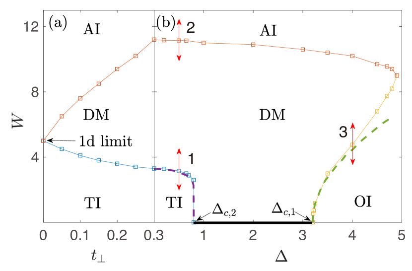
Figure 1: Phase diagram of the 3D class BDI model determined by the transfer matrix calculation of the localization length along $x$ direction ($t_{\perp}\neq 0$) and along $z$ direction ($t_{\perp}=0$) and by the self-consistent Born calculation (dotted line). (a) $W$-$t_{\perp}$ diagram ($\Delta=0$) (b) $W$-$\Delta$ diagram ($t_{\perp}=3/10$). The boundary by the square boxes is the metal-insulator transition line of the zero-energy states, while the dotted line is a critical disorder strength above which the zero-energy density of state becomes finite. The bold black line represents nodal line Dirac semimetal phase. The red double-headed arrows stand for the phase transitions we focus on in this paper. AI, DM, TI and OI stand for Anderson insulator, diffusive metal, topological band insulator and trivial band insulator phases, respectively (see the text).

In the clean limit ($W=0$), an energy-momentum dispersion of ${\mathbb{H}}$ is given by $E_{\pm}({\bm{k}})=\pm\{[\Delta+2t_{\perp}(c_{x}+c_{y})+2t^{\prime}_{\parallel}c_{z}]^{2}+4t^{2}_{\parallel}s^{2}_{z}\}^{\frac{1}{2}}$ where $c_{\mu}\equiv\cos k_{\mu}$, $s_{\mu}\equiv\sin k_{\mu}$ ($\mu=x,y,z$), ${\bm{k}}\equiv(k_{x},k_{y},k_{z})$, ${\bm{H}}({\bm{k}})|u_{\pm}({\bm{k}})\rangle=E_{\pm}({\bm{k}})|u_{\pm}({\bm{k}})\rangle$, and ${\bm{H}}({\bm{k}})$ is a Fourier-transform of ${\mathbb{H}}$ without the random potential. The two energy bands undergo a sequence of phase transitions as a function of $\Delta$. When $\Delta>\Delta_{c,1}\equiv 2|t^{\prime}_{\parallel}|+4|t_{\perp}|=16/5$, there is a finite band gap between the two energy bands (trivial band insulator phase). When $\Delta_{c,1}>\Delta>\Delta_{c,2}\equiv 2|t^{\prime}_{\parallel}|-4|t_{\perp}|=4/5$, the two bands form a close loop of band touchings at $E=0$ in the momentum space, that lies on a plane of $k_{z}=0$ (nodal line Dirac semimetal phase). On decreasing $\Delta$, the loop grows up from $(k_{x},k_{y})=(\pi,\pi)$ at $\Delta=\Delta_{c,1}$ and shrink into $(0,0)$ at $\Delta=\Delta_{c,2}$. The two energy bands form a pair of two linearly dispersive Dirac cones within a cross-sectional plane that cut the closed loop into two open lines; the loop is called as Dirac nodal line. Due to the Dirac cone, the Zak phase Zak (1989) along the $k_{z}$ axis, $i\int^{\pi}_{-\pi}\langle u_{\pm}({\bm{k}})|\partial_{k_{z}}|u_{\pm}({\bm{k}})\rangle\!\ dk_{z}$, is $\pi$ and $0$ whenever $(k_{x},k_{y})$ is inside and outside the closed loop; $(k_{x},k_{y})=(\pi,\pi)$ / $(0,0)$ is inside/outside the loop. The $\pi$ Zak phase leads to Su-Schrieffer-Heeger (SSH) zero-energy states Su et al. (1979) localized at the spatial boundary along $z$. The SSH states form a ‘drum-head’ shape zero-energy flat surface state in the surface Brillouin zone, where a boundary of the ‘drum head’ is given by a projection of the Dirac nodal line onto the surface BZ. When $\Delta<\Delta_{c,2}$, the two bands open a gap again, while the Zak phase is $\pi$ for any $(k_{x},k_{y})\in[-\pi,\pi]\times[-\pi,\pi]$; the spatial boundary along $z$ has the SSH zero modes Su et al. (1979) for any surface crystal momentum in the surface BZ (topological band insulator phase). The topological insulator phase is equivalent to the one dimenisonal (1D) topological insulator in the class BDI. Namely, by turning off $t_{\perp}$ in Eq. (2), one can adiabatically connect the topological band insulator phase to decoupled 1D models with a finite band gap at $E=0$.

Re-entrant insulator-metal transition — The 1D topological insulator in the class BDI is characterized by an integer-valued topological number ${\mathbb{Z}}$ Schnyder et al. (2008). In the clean limit, the integer corresponds to a winding number Wen and Zee (1989) between the 1D Brillouin zone for $k_{z}$ and a loop formed by two Pauli matrices in ${\bm{H}}({\bm{k}})$. The winding number of the topological insulator phase in $\Delta<\Delta_{c,2}$ is $+1$ sup . When the random pontential is weakly introduced with the BDI symmetry preserved, the topological integer remains unchanged, unless the zero-energy bulk states undergo a localization-delocalization transition. Meanwhile, the zero-energy states in strongly disordered regime should be in a localized phase with the zero topological integer (Anderson insulator phase). This indicates that between the topological band insulator phase in weakly disordered regime and the Anderson insulator phase in strongly disordered regime, there must be two-step disorder-driven quantum phase transitions: one transition from the topological band insulator to metal phases and the other from metal to the Anderson insulator phases. In the 1D limit, a metal phase cannot exist in the presence of finite disorder. Thus, the two phase transition points must collapse into a point in the limit of $t_{\perp}\rightarrow 0$. The transfer matrix calculation of the localization lengths sup confirms this global structure of the phase diagram (Fig. 1).

Effect of disorders in nodal line Dirac semimetal — The bulk DOS in the nodal line Dirac semimetal (NLDSM) vanishes linearly in $E$ at the node ($E=0$) in the clean limit. When the random potential $\varepsilon_{\bm{i}}$ with a finite disorder strength is introduced, the bulk zero-energy states acquire a finite mean-free (life) time, making the DOS at $E=0$ finite. We call this metal phase with finite zero-energy DOS as diffusive metal (DM) phase and distinguish DM phase from NLDSM phase with the vanishing zero-energy DOS.

The short-ranged random potential is a marginally relevant scaling variable around the clean-limit fixed point (NLDSM fixed point), and an infinitesimally small disorder always transforms the NLDSM phase into DM phase. To see this, note first that the degeneracy between the two energy bands is not lifted in a tangential direction along the closed loop. As a result, a tree-level scaling dimension of the momentum along the tangential direction is zero. This makes the tree-level scaling dimension of the short-ranged disorder strength to be zero. Being given by an attractive interaction in an effective action, the quenched disorder strength is always reinforced by a one-loop RG correction around the clean-limit fixed point.

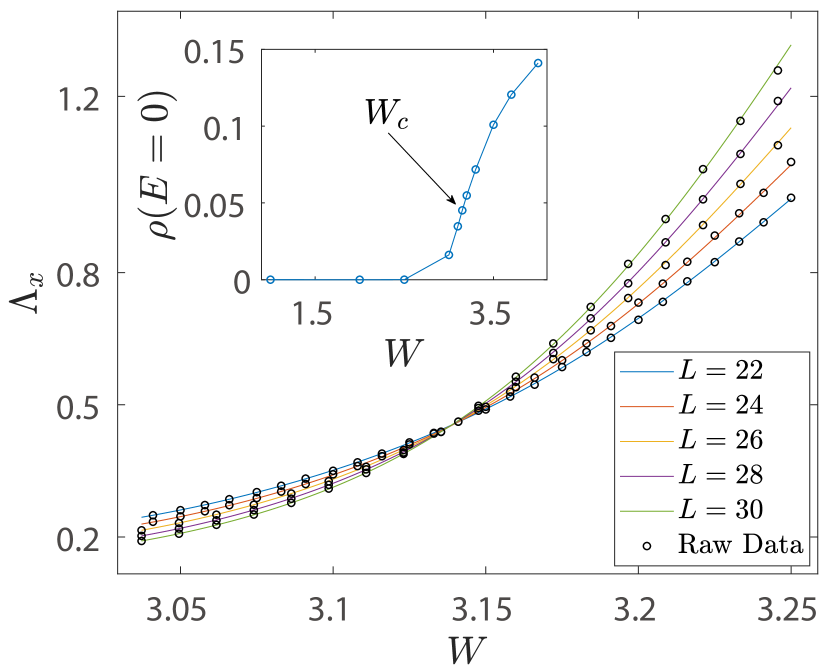
Figure 2: $\Lambda_{x}\equiv\lambda_{x}/L$ as a function of the disorder strength around the re-entrant transition between topological band insulator and diffusive metal phases in the 3D class BDI model (see phase transition 1 in Fig. 1). The circles are the raw data of $\Lambda_{x}$, where an error bar is smaller than the circle size. The curves are from the polynomial fitting results with $(m_{1},n_{1},m_{2},n_{2})$=(3,3,0,1). Inset: bulk density of states at $E=0$ near the re-entrant transition point.

The same conclusion can be reached by self-consistent Born (SCB) analysis. The SCB gives a gap equation for the mean-free time of the zero-energy eigenstates of ${\mathbb{H}}$, $\tau$, as;

$$1=K\int_{[-\pi,\pi]^{3}}\frac{d^{3}{\bm{k}}}{(2\pi)^{3}}\frac{1}{E^{2}({\bm{k}})+\tau^{-2}},$$ (3)

where $K\equiv W^{2}/12$ and $E^{2}({\bm{k}})\equiv E^{2}_{\pm}({\bm{k}})$ given above sup . The 3D momentum integral in the right hand side can be decomposed into a 1D momentum integral along the closed loop, $k_{\parallel}$, and 2D momentum integral within the cross-sectional plane, ${\bm{k}}_{\perp}$. Since $E({\bm{k}})$ has the linear dispersion around the node within the plane, the 2D integral over ${\bm{k}}_{\perp}$ has an infrared (IR) logarithmic singularity for any $k_{\parallel}$. Thus, the right hand side essentially reduces to $K\int_{1/v_{F}\tau}dk_{\perp}/k_{\perp}$. Due to the IR logarithmic singularity, the gap equation for arbitrary small $K$ always leads to a solution of a finite IR ‘cutoff’ $\tau^{-1}$ (a finite mean-free time of the zero-energy states), which results in a finite zero-energy DOS. In fact, the transfer matrix calculations do not indicate the presence of any quantum phase transition from NLDSM phase to DM phase at finite disorder strength (Fig. 1).

Critical exponent in the re-entrant transition– The critical exponent associated with the Anderson transition between the DM and Anderson insulator phases (phase transition 2 in Fig. 1) is evaluated by the polynomial fitting analysis of the normalized localization length as $\nu=0.80\pm 0.02$, where a localization length along the $x$ direction $\lambda_{x}$ is calculated sup . The critical exponent associated with the Anderson transition between the trivial band insulator and DM phases (phase transition 3 in Fig. 1) is evaluated as $\nu=0.82\pm 0.01$. Since the 95 $\%$ confidence intervals of these two exponents (see Table 1) overlap with each other, we conclude that the critical exponent of the Anderson transition in the 3D class BDI is $\nu=0.80\pm 0.02$.

Based on this new knowledge, we next evaluate the critical exponent associated with the re-entrant insulator-metal transition between topological band insulator and DM phases (phase transition 1 in Fig. 1). We use the same polynomial fitting analyses for the localization length along the $x$ direction $\lambda_{x}$ with $L_{x}=3\times 10^{6}$ for $L=22$, and $L_{x}=2\times 10^{6}$ for $L=24,26,28,30$ (Fig. 2). The fitting result with GOF greater than 0.1 gives $\nu=0.83\pm 0.05$ (Table. 1). From the comparison with the other two exponents from the phase transitions 2 and 3, we conclude that the re-entrant transition between the topological band insulator and DM phases is of the same universality class as the Anderson transition in 3D class BDI. Note also that the KPE calculation shows a finite zero-energy DOS on the re-entrant phase transition point (inset of Fig. 2). The situation is similar to previous studies on 2D symplectic class, where the quantum spin Hall insulator to DM transition shows the same critical exponent as in standard Wigner-Dyson (WD) universality classes  Obuse et al. (2007); Fu and Kane (2012) and to a previous study on 3D unitary class, where the layered Chern insulator to DM transition shows the same critical exponent as in the WD universality classes Luo et al. (2018a).

Summary — The critical exponents of Anderson transitions in 3D class CI and that in class BDI are clarified numerically. A disorder-driven re-entrant transition from a topological band insulator phase to diffusive metal phase is studied in a model of the class BDI. A comparison of the critical exponents suggests that the re-entrant transition belongs to the same universality class as the Anderson transition in the class BDI. The transfer-matrix calculation as well as self-consistent Born study suggests that an infinitesimally small disorder drives the nodal line Dirac semimetal in the clean limit to the diffusive metal.

Acknowledgment — This work (X. L., B. X. and R. S.) was supported by NBRP of China Grants No. 2014CB920901, No. 2015CB921104, and No. 2017A040215. T. O. was supported by JSPS KAKENHI Grants No. JP15H03700 and 19H00658.

I supplemental materials

I.1 3D class CI model

The tight-binding model Hamiltonian for the 3D class CI model in the clean limit reduces to the following two by two Hamiltonian in the momentum space,

$${\bm{H}}({\bm{k}})=2t_{\perp}(\cos k_{x}+\cos k_{y})\sigma_{0}+t_{\parallel}\sigma_{1}+(2t^{\prime}_{\parallel}\cos k_{z}+\Delta)\sigma_{3},$$ (4)

with two separate energy bands,

$$E_{\pm}({\bm{k}})=2t_{\perp}(\cos k_{x}+\cos k_{y})\pm\sqrt{t^{2}_{\parallel}+(2t^{\prime}_{\parallel}\cos k_{z}+\Delta)^{2}}.$$ (5)

In the main text, we set $\Delta=t_{\parallel}=t^{\prime}_{\parallel}=t_{\perp}=1$, where the zero-energy states comprise of two disconnected Fermi surfaces (Fig. 3). In the presence of the random potential, the localization length of the zero-energy eigenstates ($\lambda_{z}$) is calculated along $z$ direction as a function of disorder strength $W$, where the periodic boundary condition is imposed along $x$ and $y$ directions. A linear dimension of a cross-section of the cubic lattice within the $xy$ plane ($L$) and a linear dimension along the $z$ direction ($L_{z}$) are set to $L_{z}=2\times 10^{6}$ for $L=24,28$ and $L_{z}=4\times 10^{6}$ for $L=8,10,\cdots,18,20$, respectively. On increasing the disorder strength, the zero-energy eigenstates undergo the Anderson transition, where the critical disorder strength is identified by a scale-invariant point of the normalized localization length $\Lambda_{z}\equiv\lambda_{z}/L$ (Fig. 4). The density of states (DOS) of the system with the random pontential is also calculated as a function of the disorder strength $W$ in terms of the Kernel polynomial expansion (KPE) method Weiße et al. (2006) for the same set of the tight-binding parameters (Fig. 5). For any $W$, the total DOS is an even function in $E$ due to the particle-hole symmetry, while a tiny odd component in $E$ stems from finite expansion order in the KPE method. The zero-energy DOS decreases on increasing the disorder strength $W$, while it remains finite at the Anderson transition point ($W_{c}\simeq 11$; right panel of Fig. 5).

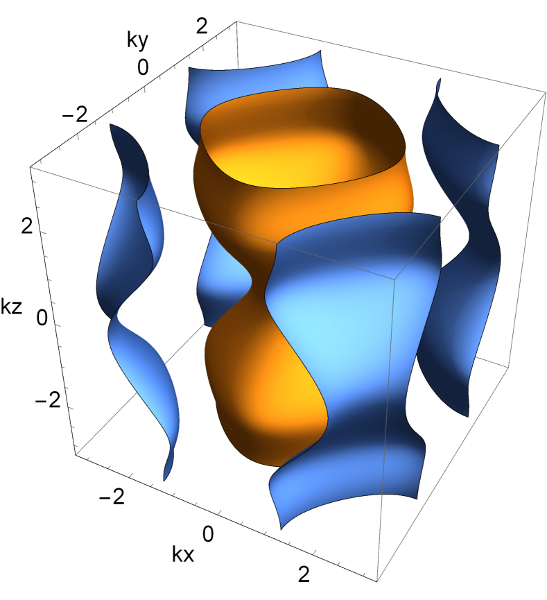
Figure 3: two Fermi surfaces at $E=0$ in the 3D class CI model.

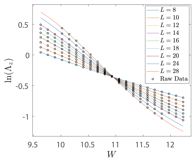
Figure 4: $\ln(\Lambda_{z})\equiv\ln(\lambda_{z}/L)$ as a function of the disorder strength $W$ for the 3D class CI model. The circles are the raw data of $\ln(\Lambda_{z})$, whose error bar is smaller than the circle size. The curves are from the fitting results with the Taylor-expansion orders:$(m_{1},n_{1},m_{2},n_{2})$=(2,3,0,1).

Figure 5: (left) density of states (DOS) as a function of $E$ for several different values of the disorder strength $W$. (right) The zero-energy DOS as a function of the disorder strength. The density of states is calculated by the kernel polynomial expansion method Weiße et al. (2006) with a cubic system size $L=100$ and large polynomial expansion order ($N$=4000). The DOS is averaged over 20 different disorder realizations.

I.2 3D class BDI model

The tight-binding Hamiltonian for 3D class BDI model in the clean limit is given by the following 2 by 2 Hamiltonian,

$${\bm{H}}({\bm{k}})=a_{2}({\bm{k}})\sigma_{2}+a_{3}({\bm{k}})\sigma_{3}$$ (6)

with

$$a_{2}({\bm{k}}) =2t_{\parallel}\sin k_{z},$$

$$a_{3}({\bm{k}}) =\Delta+2t_{\perp}(\cos k_{x}+\cos k_{y})+2t^{\prime}_{\parallel}\cos k_{z}.$$

I.2.1 self-consistent Born analyses in favor for single-particle Green function

A single-particle retarded/advanced Green function is averaged over the random potential $\varepsilon_{\bm{i}}$;

$$[{\bm{G}}_{\pm}(E,{\bm{k}},{\bm{k}}^{\prime})]_{c,c^{\prime}}=$$

$$\ \ \frac{1}{N}\sum_{{\bm{i}},{\bm{j}}}e^{i{\bm{k}}{\bm{i}}-i{\bm{k}}^{\prime}{\bm{j}}}\bigg{\langle}\bigg{[}\frac{1}{E-{\mathbb{H}}_{0}-{\mathbb{V}}\pm i\delta}\bigg{]}_{({\bm{i}},c|{\bm{j}},c^{\prime})}\bigg{\rangle}_{\rm imp}$$ (7)

where $c,c^{\prime}$ denotes the index for the two orbitals, $c,c^{\prime}=a,b$. ${\mathbb{H}}_{0}$ is ${\mathbb{H}}$ without the random potential and ${\mathbb{V}}$ is the random potential part,

$$\big{[}{\mathbb{V}}\big{]}_{({\bm{i}},c|{\bm{j}},c^{\prime})}\equiv\delta_{{\bm{i}},{\bm{j}}}[\sigma_{3}]_{c,c^{\prime}}\varepsilon_{\bm{i}}.$$ (8)

$\langle\cdots\rangle_{\rm imp}$ stands for a quenched average over the short-ranged random potential and is defined below;

$$\langle\varepsilon_{\bm{i}}\varepsilon_{\bm{j}}\rangle_{\rm imp} =\delta_{{\bm{i}},{\bm{j}}}\bigg{(}\int^{W/2}_{-W/2}\varepsilon^{2}d\varepsilon\bigg{)}\Bigg{/}\bigg{(}\int^{W/2}_{-W/2}d\varepsilon\bigg{)}$$

$$=\delta_{{\bm{i}},{\bm{j}}}\frac{W^{2}}{12}\equiv\delta_{{\bm{i}},{\bm{j}}}K.$$ (9)

In the thermodynamic limit, the quenched average of higher-order powers in the random potential is given by the second-order average, e.g.

$$\langle\varepsilon_{\bm{i}}\varepsilon_{\bm{j}}\varepsilon_{\bm{n}}\varepsilon_{\bm{m}}\rangle_{\rm imp}=$$

$$\ \ (\delta_{{\bm{i}},{\bm{j}}}\delta_{{\bm{n}},{\bm{m}}}+\delta_{{\bm{i}},{\bm{n}}}\delta_{{\bm{j}},{\bm{m}}}+\delta_{{\bm{i}},{\bm{m}}}\delta_{{\bm{j}},{\bm{n}}})(K^{2}+{\cal O}(N^{-1})).$$ (10)

The averaged Green function takes a diagonal form in the momentum; $[{\bm{G}}_{\pm}(E,{\bm{k}},{\bm{k}}^{\prime})]_{c,c^{\prime}}=\delta_{{\bm{k}},{\bm{k}}^{\prime}}[{\bm{G}}_{\pm}(E,{\bm{k}})]_{c,c^{\prime}}$, where the two by two $[{\bm{G}}_{\pm}(E,{\bm{k}})]$ is given by the following Dyson equation within the self-consistent Born approximation,

$${\bm{G}}_{\pm}(E,{\bm{k}}) ={\bm{G}}_{\pm,0}(E,{\bm{k}})$$

$$\bigg{(}{\bm{1}}+\frac{K}{N}\sum_{\bm{q}}\sigma_{3}{\bm{G}}_{\pm}(E,{\bm{q}})\sigma_{3}\!\ {\bm{G}}_{\pm}(E,{\bm{k}})\bigg{)}.$$ (11)

${\bm{G}}_{\pm,0}(E,{\bm{k}})$ is the Green function in the clean limit;

$${\bm{G}}^{-1}_{\pm,0}(E,{\bm{k}}) =(E\pm i\delta)-{\bm{H}}({\bm{k}})$$

$$\equiv a_{0}\sigma_{0}-a_{2}({\bm{k}})\sigma_{2}-a_{3}({\bm{k}})\sigma_{3}$$ (12)

with $a_{0}\equiv E\pm i\delta$. The solution of the Dyson equation is characterized by two ${\bm{k}}$-independent complex-valued constants, $\gamma_{0}$ and $\gamma_{3}$;

$${\bm{G}}^{-1}_{\pm}(E,{\bm{k}})=\big{(}a_{0}-\gamma_{0}\big{)}\sigma_{0}-a_{2}({\bm{k}})\sigma_{2}-\big{(}a_{3}({\bm{k}})+\gamma_{3}\big{)}\sigma_{3}.$$ (13)

For the zero-energy states ($E=0$), $\gamma_{0}$ and $\gamma_{3}$ take pure imaginary and real values respectively;

$${\rm Im}\gamma_{0} =\frac{K}{N}\sum_{\bm{q}}\frac{{\rm Im}\gamma_{0}}{a^{2}_{2}({\bm{q}})+(a_{3}({\bm{q}})+{\rm Re}\gamma_{3})^{2}+({\rm Im}\gamma_{0})^{2}},$$ (14)

$${\rm Re}\gamma_{3} =-\frac{K}{N}\sum_{\bm{q}}\frac{a_{3}({\bm{q}})+{\rm Re}\gamma_{3}}{a^{2}_{2}({\bm{q}})+(a_{3}({\bm{q}})+{\rm Re}\gamma_{3})^{2}+({\rm Im}\gamma_{0})^{2}}.$$ (15)

${\rm Re}\gamma_{3}$ renormalizes an energy gap in the band insulator phases as well as a shape of nodal line in the semimetal phase. ${\rm Im}\gamma_{0}$ is an inverse of a mean-free (life) time of the zero-energy states. According to the gap equations, ${\rm Im}\gamma_{0}$ can be either zero (‘ballistic’ zero-energy-states solution) or a finite constant that satisfies Eq. (15) and

$$1 =\frac{K}{N}\sum_{\bm{q}}\frac{1}{a^{2}_{2}({\bm{q}})+(a_{3}({\bm{q}})+{\rm Re}\gamma_{3})^{2}+({\rm Im}\gamma_{0})^{2}}.$$ (16)

Eq. (16) corresponds to Eq. (3) in the main text. The zero-energy density of states is proportional to ${\rm Im}\gamma_{0}$;

$$\rho(E=0)=-\frac{1}{\pi}\frac{1}{N}\sum_{\bm{k}}{\rm Im}{\rm Tr}\big{[}{\bm{G}}_{+}(E=0,{\bm{k}})\big{]}=\frac{2{\rm Im}\gamma_{0}}{\pi K}.$$ (17)

By solving the gap equations numerically, we determine a phase boundary of $\rho(E=0)$; a boundary between a phase with $\rho(E=0)=0$ and a phase with $\rho(E=0)\neq 0$ (Fig. 1 in the main text).

I.2.2 localization length and density of states

The localization length along $x$ ($\lambda_{x}$) is calculated as a function of disorder strength $W$ at three different parameter points of the 3D class BDI model. In the calculation, following three quantum phase transition points $W_{c}$ are identified with scale-invariant points of the normalized localization length $\Lambda_{x}\equiv\lambda_{x}/L$: (i) phase transition 1 between the topological band insulator and DM phases; $\Delta=0.5$ and $W_{c}=3.135$ (Fig. 2 in the main text), (ii) phase transition 2 between the DM and AI phases; $\Delta=0.5$ and $W_{c}=11.96$ (left panel of Fig. 6), and (iii) phase transition 3 between the trivial band insulator and DM phases; $\Delta=4.0$ and $W_{c}=4.76$ (right panel of Fig. 6). Here $L$ and $L_{x}$ are a linear dimension of the cubic lattice system within the $yz$ plane and along $x$ respectively. For the phase transition 2, the localization length $\lambda_{x}$ is calculated with $L_{x}=2\times 10^{6}$ for $L=26$ and $L_{x}=1\times 10^{6}$ for $L=14,\!\ 16,\!\ 18,\!\ 20,\!\ 22,\!\ 24$. For the phase transition 3, $\lambda_{x}$ is calculated with $L_{x}=3\times 10^{6}$ for $L=22$ and $L_{x}=2\times 10^{6}$ for $L=24,\!\ 26,\!\ 28,\!\ 30$. From the polynomial fitting analyses, the critical exponent of 3D calss BDI as well as the MI transition points $W_{c}$ are precisely determined (Table I in the main text).

The DOS is also calculated for the same sets of parameters in terms of the KPE method (Fig. 7). The zero-energy DOS is always finite at the MI transition points of the three phase transitions. Especially for the phase transitions 1 and 3, the zero-energy DOS becomes finite at a certain critical disorder strength below $W_{c}$. The critical disorder strengths for the phase transitions 1 and 3 are consistent with the boundary determined by the self-consistent Born analyses.

Figure 6: Localization length as a function of the disorder strength in the 3D class BDI model. left: $\Lambda_{x}\equiv\lambda_{x}/L$ for the phase transition 2 (see in Fig. 1 in the main text). right: $\ln(\Lambda_{x})\equiv\ln(\lambda_{x}/L)$ for the phase transition 3 (see in Fig. 1 in the main text). The circles are the raw data, where an error bar is smaller than the circle size. The curves are from the polynomial fitting curves with $(m_{1},n_{1},m_{2},n_{2})$=(3,3,0,1) (left) and with $(m_{1},n_{1},m_{2},n_{2})$=(2,3,0,1) (right).

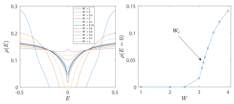
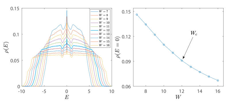
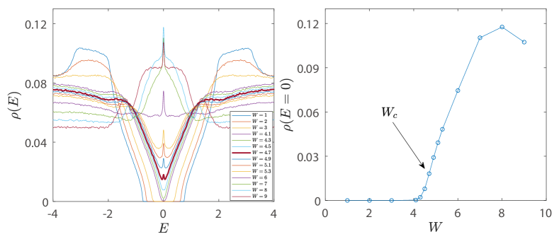
Figure 7: Density of states (DOS) by the kernel polynomial expansion method Weiße et al. (2006) with the cubic system size $L=100$ around the three quantum phase transition points. upper: DOS for the phase transition 1 with the polynomial expansion order $N$=3000; middle:DOS for the phase transition 2 with the polynomial expansion order $N$=2000; lower:DOS for the phase transition 3 with the polynomial expansion order $N$=4000. (Left) DOS as a function of $E$ and (right) the zero-energy DOS as a function of the disorder strength $W$. We take an average over four different disorder realizations with fixed $W$. The bold line in the left figures indicate a disorder strength that is closest to $W_{c}$.

I.2.3 one dimensional limit

When $t_{\perp}=0$, the 3D class BDI model reduces to a one-dimensional (1D) model;

$${\bm{H}}({\bm{k}}) =2t_{\parallel}\sin k_{z}\sigma_{2}+(\Delta+2t^{\prime}_{\parallel}\cos k_{z})\sigma_{3}$$

$$=\sqrt{(2t_{\parallel}\sin k_{z})^{2}+(\Delta+2t^{\prime}_{\parallel}\cos k_{z})^{2}}$$

$$\hskip 56.9055pt\times\big{(}n_{2}(k_{z})\sigma_{2}+n_{3}(k_{z})\sigma_{3}\big{)}.$$ (18)

The topological integer for the 1D BDI topological insulator is defined as a winding number of the two-component unit vector $(n_{2}(k_{z}),n_{3}(k_{z}))$ as a function of $k_{z}\in[-\pi,\pi]$;

$${\mathbb{Z}}\equiv\int^{\pi}_{-\pi}\frac{dk_{z}}{2\pi}\Big{(}n_{3}\partial_{k_{z}}n_{2}-n_{2}\partial_{k_{z}}n_{3}\Big{)}.$$ (19)

When $|\Delta|<2|t^{\prime}_{\parallel}|$ with $t_{\parallel}\neq 0$, the integer is $\pm 1$, while the integer is zero for $|\Delta|>2|t^{\prime}_{\parallel}|$ with $t_{\parallel}\neq 0$. The topological integers of the topological phase in Fig. 1 in the main text are $+1$ for any $k_{x}$ and $k_{y}$.

When the random potential is weakly introduced with the BDI symmetry, the topological integer remains unchanged, unless the zero-energy bulk states become delocalized. On the one hand, the bulk eigenstates in the strongly disorder regime must be in a conventional localized phase with the zero topological integer. This suggests that between the 1D BDI topological insulator phase in the weakly disordered regime and 1D conventional localized phase in the strongly disordered regime, there must be a insulator to insulator transition at a certain disorder strength. To test this numerically, we set $t_{\perp}=0$ and calculate a 1D localization length $\xi_{\mathrm{1d}}$ for $\Delta=0,t_{\parallel}^{\prime}=-1$ and $t_{\parallel}=-1/4$ (Fig. 8). The localization length shows a very strong peak around $W\simeq 5.0$, indicating a certain transition from 1D topological insulator phase to Anderson insulator phase. The point named as ‘1d limit’ in Fig. 1 in the main text is determined by the value of $W$ at which $\xi_{\rm 1d}$ shows the sharp peak. Numerically, however, the peak value remains finite even for very large $L_{z}\simeq 10^{8}$. We leave it for future study a detailed behaviour of $\xi_{\rm 1d}$ in this one-dimensional limit.

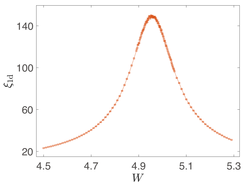
Figure 8: 1D localization length $\xi_{\mathrm{1d}}$ as a function of the disorder strength $W$ for $\Delta=t_{\perp}=0$, $t_{\parallel}=-1$, and $t^{\prime}_{\parallel}=-1/4$. 1D BDI topological insulator phase is separated from the Anderson insulator at a point around $W\simeq 5.0$, where the localization length shows a very strong peak.

References

- Cardy (1996) J. Cardy, Scaling and Renormalization in Statistical Physics (Cambridge University Press, 1996).
- Anderson (1958) P. W. Anderson, Phys. Rev. 109, 1492 (1958).
- Wegner (1976) F. J. Wegner, Zeitschrift für Physik B Condensed Matter 25, 327 (1976).
- Abrahams et al. (1979) E. Abrahams, P. W. Anderson, D. C. Licciardello, and T. V. Ramakrishnan, Phys. Rev. Lett. 42, 673 (1979).
- Effetov et al. (1980) K. B. Effetov, A. I. Larkin, and D. E. Khmel’nitsukii, Soviet Phys. JETP 52, 568 (1980).
- Hikami (1981) S. Hikami, Phys. Rev. B 24, 2671 (1981).
- Pichard and Sarma (1981) J.-L. Pichard and G. Sarma, J. Phys. C: Solid State Phys. C14, L127 (1981).
- MacKinnon and Kramer (1981) A. MacKinnon and B. Kramer, Phys. Rev. Lett. 47, 1546 (1981).
- MacKinnon and Kramer (1983) A. MacKinnon and B. Kramer, Zeitschrift für Physik B Condensed Matter 53, 1 (1983).
- Xu et al. (2015) S.-Y. Xu, I. Belopolski, N. Alidoust, M. Neupane, G. Bian, C. Zhang, R. Sankar, G. Chang, Z. Yuan, C.-C. Lee, S.-M. Huang, H. Zheng, J. Ma, D. S. Sanchez, B. K. Wang, F.-C. Bansil, A.; Chou, P. P. Shibayev, H. Lin, S. Jia, and M. Z. Hasan, Science 349, 613 (2015).
- Lv et al. (2015) B. Q. Lv, H. M. Weng, B. B. Fu, X. P. Wang, H. Miao, J. Ma, P. Richard, X. C. Huang, L. X. Zhao, G. F. Chen, Z. Fang, X. Dai, T. Qian, and H. Ding, Phys. Rev. X 5, 031013 (2015).
- Yan and Felser (2017) B. Yan and C. Felser, Annual Review of Condensed Matter Physics 8, 337 (2017).
- Armitage et al. (2018) N. P. Armitage, E. J. Mele, and A. Vishwanath, Reviews of Modern Physics 90 (2018), 10.1103/RevModPhys.90.015001.
- Lou et al. (2016) R. Lou, J.-Z. Ma, Q.-N. Xu, B.-B. Fu, L.-Y. Kong, Y.-G. Shi, P. Richard, H.-M. Weng, Z. Fang, S.-S. Sun, Q. Wang, H.-C. Lei, T. Qian, H. Ding, and S.-C. Wang, Phys. Rev. B 93, 241104 (2016).
- Takane et al. (2016) D. Takane, Z. Wang, S. Souma, K. Nakayama, C. X. Trang, T. Sato, T. Takahashi, and Y. Ando, Phys. Rev. B 94, 121108 (2016).
- Bian et al. (2016) G. Bian, T.-R. Chang, R. Sankar, S.-Y. Xu, H. Zheng, T. Neupert, C.-K. Chiu, S.-M. Huang, G. Chang, I. Belopolski, D. S. Sanchez, M. Neupane, N. Alidoust, C. Liu, B. Wang, C.-C. Lee, H.-T. Jeng, C. Zhang, Z. Yuan, S. Jia, A. Bansil, F. Chou, H. Lin, and M. Z. Hasan, Nature Communications 7, 10556 (2016).
- Schoop et al. (2016) L. M. Schoop, M. N. Ali, C. Straßer, A. Topp, A. Varykhalov, D. Marchenko, V. Duppel, S. S. P. Parkin, B. V. Lotsch, and C. R. Ast, Nature Communications 7, 11696 (2016).
- Hosen et al. (2017) M. M. Hosen, K. Dimitri, I. Belopolski, P. Maldonado, R. Sankar, N. Dhakal, G. Dhakal, T. Cole, P. M. Oppeneer, D. Kaczorowski, F. Chou, M. Z. Hasan, T. Durakiewicz, and M. Neupane, Phys. Rev. B 95, 161101 (2017).
- Wang et al. (2017) X.-B. Wang, X.-M. Ma, E. Emmanouilidou, B. Shen, C.-H. Hsu, C.-S. Zhou, Y. Zuo, R.-R. Song, S.-Y. Xu, G. Wang, L. Huang, N. Ni, and C. Liu, Phys. Rev. B 96, 161112 (2017).
- Liu et al. (2018) Z. Liu, R. Lou, P. Guo, Q. Wang, S. Sun, C. Li, S. Thirupathaiah, A. Fedorov, D. Shen, K. Liu, H. Lei, and S. Wang, Phys. Rev. X 8, 031044 (2018).
- Syzranov et al. (2015a) S. V. Syzranov, V. Gurarie, and L. Radzihovsky, Phys. Rev. B 91, 035133 (2015a).
- Syzranov et al. (2015b) S. V. Syzranov, L. Radzihovsky, and V. Gurarie, Phys. Rev. Lett. 114, 166601 (2015b).
- Syzranov and Radzihovsky (2018) S. V. Syzranov and L. Radzihovsky, Annual Review of Condensed Matter Physics 9, 35 (2018), https://doi.org/10.1146/annurev-conmatphys-033117-054037 .
- Kobayashi et al. (2014) K. Kobayashi, T. Ohtsuki, K.-I. Imura, and I. F. Herbut, Phys. Rev. Lett. 112, 016402 (2014).
- Sbierski et al. (2014) B. Sbierski, G. Pohl, E. J. Bergholtz, and P. W. Brouwer, Phys. Rev. Lett. 113, 026602 (2014).
- Sbierski et al. (2015) B. Sbierski, E. J. Bergholtz, and P. W. Brouwer, Phys. Rev. B 92, 115145 (2015).
- Pixley et al. (2015) J. H. Pixley, P. Goswami, and S. Das Sarma, Phys. Rev. Lett. 115, 076601 (2015).
- Pixley et al. (2016) J. H. Pixley, D. A. Huse, and S. Das Sarma, Phys. Rev. X 6, 021042 (2016).
- Liu et al. (2016) S. Liu, T. Ohtsuki, and R. Shindou, Phys. Rev. Lett. 116, 066401 (2016).
- Luo et al. (2018a) X. Luo, B. Xu, T. Ohtsuki, and R. Shindou, Phys. Rev. B 97, 045129 (2018a).
- Luo et al. (2018b) X. Luo, T. Ohtsuki, and R. Shindou, Phys. Rev. B 98, 020201 (2018b).
- Gade and Wegner (1991) R. Gade and F. Wegner, Nuclear Physics B 360, 213 (1991).
- Gade (1993) R. Gade, Nuclear Physics B 398, 499 (1993).
- Altland and Zirnbauer (1997) A. Altland and M. R. Zirnbauer, Phys. Rev. B 55, 1142 (1997).
- Schnyder et al. (2008) A. P. Schnyder, S. Ryu, A. Furusaki, and A. W. W. Ludwig, Phys. Rev. B 78, 195125 (2008).
- Obuse et al. (2007) H. Obuse, A. Furusaki, S. Ryu, and C. Mudry, Phys. Rev. B 76, 075301 (2007).
- Fu and Kane (2012) L. Fu and C. L. Kane, Physical Review Letters 109 (2012), 10.1103/PhysRevLett.109.246605.
- García-García and Cuevas (2006) A. M. García-García and E. Cuevas, Physical Review B 74 (2006), 10.1103/PhysRevB.74.113101.
- Gonçalves et al. (2019) M. Gonçalves, P. Ribeiro, E. V. Castro, and M. A. N. Araújo, “Disorder driven multifractality transition in weyl nodal loops,” (2019), arXiv:1908.06910 [cond-mat.dis-nn] .
- (40) See Supplemental Material at [URL will be inserted by publisher].
- Slevin and Ohtsuki (2014) K. Slevin and T. Ohtsuki, New Journal of Physics 16, 015012 (2014).
- Weiße et al. (2006) A. Weiße, G. Wellein, A. Alvermann, and H. Fehske, Rev. Mod. Phys. 78, 275 (2006).
- Slevin and Ohtsuki (1997) K. Slevin and T. Ohtsuki, Phys. Rev. Lett. 78, 4083 (1997).
- Asada et al. (2005) Y. Asada, K. Slevin, and T. Ohtsuki, Journal of the Physical Society of Japan 74, 238 (2005), https://doi.org/10.1143/JPSJS.74S.238 .
- Zak (1989) J. Zak, Phys. Rev. Lett. 62, 2747 (1989).
- Su et al. (1979) W. P. Su, J. R. Schrieffer, and A. J. Heeger, Phys. Rev. Lett. 42, 1698 (1979).
- Wen and Zee (1989) X. Wen and A. Zee, Nuclear Physics B 316, 641 (1989).