A Fast and Compact Invertible Sketch for Network-Wide Heavy Flow Detection

Abstract

Fast detection of heavy flows (e.g., heavy hitters and heavy changers) in massive network traffic is challenging due to the stringent requirements of fast packet processing and limited resource availability. Invertible sketches are summary data structures that can recover heavy flows with small memory footprints and bounded errors, yet existing invertible sketches incur high memory access overhead that leads to performance degradation. We present MV-Sketch, a fast and compact invertible sketch that supports heavy flow detection with small and static memory allocation. MV-Sketch tracks candidate heavy flows inside the sketch data structure via the idea of majority voting, such that it incurs small memory access overhead in both update and query operations, while achieving high detection accuracy. We present theoretical analysis on the memory usage, performance, and accuracy of MV-Sketch in both local and network-wide scenarios. We further show how MV-Sketch can be implemented and deployed on P4-based programmable switches subject to hardware deployment constraints. We conduct evaluation in both software and hardware environments. Trace-driven evaluation in software shows that MV-Sketch achieves higher accuracy than existing invertible sketches, with up to 3.38$\times$ throughput gain. We also show how to boost the performance of MV-Sketch with SIMD instructions. Furthermore, we evaluate MV-Sketch on a Barefoot Tofino switch and show how MV-Sketch achieves line-rate measurement with limited hardware resource overhead.

I Introduction

Identifying abnormal patterns of flows (e.g., hosts, source-destination pairs, or 5-tuples) in massive network traffic is essential for various network management tasks, such as traffic engineering [8], load balancing [2] and intrusion detection [21]. Two types of abnormal flows are of particular interest: heavy hitters (i.e., flows that generate an unexpectedly high volume of traffic) and heavy changers (i.e., flows that generate an unexpectedly high change of traffic volume in a short duration). By identifying both heavy hitters and heavy changers (collectively referred to as heavy flows), network operators can quickly respond to performance outliers, mis-behaved usage, and potential DDoS attacks, so as to maintain network stability and QoS guarantees.

Unfortunately, the stringent requirements of fast packet processing and limited memory availability pose challenges to practical heavy flow detection. First, the packet processing rate of heavy flow detection must keep pace with the ever-increasing network speed, especially in the worst case when traffic bursts or attacks happen [25]. For example, a fully utilized 10 Gb/s link with a minimum packet size of 64 bytes implies that the heavy flow detection algorithm must process at least 14.88M packets per second. In addition, the available memory footprints are constrained in practice (e.g., less than 2 MB of SRAM per stage in emerging programmable switches [11, 43]). While per-flow monitoring with linear hash tables is arguably feasible in software [1], its performance degrades once the working set grows beyond the available software cache capacity.

Given the rigid packet processing and memory requirements, many approaches perform approximate heavy flow detection via sketches, which are summary data structures that significantly mitigate memory footprints with bounded detection errors. Classical sketches [16, 15, 31] are proven effective, but are non-invertible: while we can query a sketch whether a specific flow is a heavy flow, we cannot readily recover all heavy flows from only the sketch itself. Instead, we must check whether every possible flow is a heavy flow. Such a brute-force approach is computationally expensive for an extremely large flow key space (e.g., the size is $2^{104}$ for 5-tuple flows).

This motivates us to explore invertible sketches, which provide provable error bounds as in classical sketches, while supporting the queries of recovering all heavy flows. Invertible sketches are well studied in the literature (e.g., [16, 18, 40, 13, 33, 26]) for heavy flow detection. However, there remain limitations in existing invertible sketches. In particular, they either maintain heavy flows in external DRAM-based data structures [16, 26], or track flow keys in smaller-size bits or sub-keys [18, 40, 13, 33]. We argue that both approaches incur substantial memory access overhead that leads to degraded processing performance (Section II-B).

In this paper, we present MV-Sketch, a fast and compact invertible sketch for heavy flow detection. It tracks candidate heavy flow keys together with the counters in a sketch data structure, and updates the candidate heavy flow keys based on the majority vote algorithm [12] in an online streaming fashion. A key design feature of MV-Sketch is that it maintains a sketch data structure with small and static memory allocation (i.e., no dynamic memory allocation is needed). This not only allows lightweight memory access in both update and detection operations, but also provides viable opportunities for hardware acceleration and feasible deployment in hardware switches. To summarize, we make the following contributions.

• We design MV-Sketch, an invertible sketch that supports both heavy hitter and heavy changer detection and can be generalized for distributed detection, including both scalable detection (which provides scalability) and network-wide detection (which provides a network-wide view of measurement results). See Section III.

• We present theoretical analysis on MV-Sketch for its memory space complexity, update/detection time complexity, and detection accuracy. See Section IV.

• We present the implementation of MV-Sketch on P4-based programmable switches [10] subject to various hardware deployment constraints. See Section V.

• We conduct evaluation in both software and hardware environments. We show via trace-driven evaluation in software that MV-Sketch achieves higher detection accuracy for most memory configurations and up to 3.38$\times$ throughput gain over state-of-the-art invertible sketches. We also extend MV-Sketch with Single Instruction, Multiple Data (SIMD) instructions to boost its update performance. Furthermore, we prototype MV-Sketch in the P4 language [10] and compile it to the Barefoot Tofino chipset [45]. MV-Sketch achieves line-rate measurement with limited resource overhead. It also achieves higher accuracy and smaller resource usage than PRECISION [7] (a heavy hitter detection scheme in programmable switches). See Section VI.

The source code of MV-Sketch (including the software implementation and the P4 code) is available for download at: http://adslab.cse.cuhk.edu.hk/software/mvsketch.

II Background

II-A Heavy Flow Detection

We consider a stream of packets, each of which is denoted by a key-value pair $(x,v_{x})$, where $x$ is a key drawn from a domain $[n]=\{0,1,\cdots,n-1\}$ and $v_{x}$ is the value of $x$. In network measurement, $x$ is the flow identifier (e.g., source/destination address pairs or 5-tuples), while $v_{x}$ is either one (for packet counting) or the packet size (for byte counting). We conduct measurement at regular time intervals called epochs.

We formally define heavy hitters and heavy changers as follows. Let $\phi$ be a pre-defined fractional threshold (where $0<\phi<1$) that is used to differentiate heavy flows from network traffic (we use the same $\phi$ for both heavy hitter and heavy changer detection for simplicity). Let $S(x)$ be the sum (of all $v_{x}$’s) of flow $x$ in an epoch, and $D(x)$ be the absolute change of $S(x)$ of flow $x$ across two epochs. Let $\mathcal{S}$ be the total sum of all flows in an epoch (i.e., $\mathcal{S}=\sum_{x\in[n]}S(x)$), and $\mathcal{D}$ be the total absolute change of all flows across two epochs (i.e., $\mathcal{D}=\sum_{x\in[n]}D(x)$). Both $\mathcal{S}$ and $\mathcal{D}$ can be obtained in practice: for $\mathcal{S}$, we can maintain an extra counter that counts the total traffic; for $\mathcal{D}$, we can run an $l_{1}$-streaming algorithm and estimate $\mathcal{D}$ (equivalent to the $l_{1}$-distance) in one pass [37]. Finally, flow $x$ is said to be a heavy hitter if $S(x)\geq\phi\mathcal{S}$, or a heavy changer if $D(x)\geq\phi\mathcal{D}$.

II-B Sketches

Sketches are summary data structures that track values in a fixed number of entries called buckets. Classical sketches on heavy flow detection (e.g., Count Sketch [15], K-ary Sketch [31], and Count-Min Sketch [16]) represent a sketch as a two-dimensional array of buckets and provide different theoretical trade-offs across memory usage, performance, and accuracy.

Take Count-Min Sketch [16] as an example. We construct the sketch as $r$ rows of $w$ buckets each. Each bucket is associated with a counter initialized as zero. For each tuple $(x,v_{x}$) received in an epoch, we hash $x$ into a bucket in each of the $r$ rows using $r$ pairwise independent hash functions. We increment the counter in each of the $r$ hashed buckets by $v_{x}$. Since multiple flows can be hashed to the same bucket, we can only provide an estimate for the sum of a flow. Count-Min Sketch uses the minimum counter value of all $r$ hashed buckets as the estimated sum of a flow. We can check if a flow is a heavy hitter by checking if its estimated sum exceeds the threshold; similarly, we can check if a flow is a heavy changer by checking if the absolute change of its estimated sums in two epochs exceeds the threshold. However, Count-Min Sketch is non-invertible, as we must check every flow in the entire flow key space to recover all heavy flows; note that Count Sketch and K-ary Sketch are also non-invertible.

Invertible sketches (e.g., [18, 16, 13, 40, 26, 33]) allow all heavy flows to be recovered from only the sketch data structure itself. State-of-the-art invertible sketches can be classified into three types.

Extra data structures. Count-Min-Heap [16] is an augmented Count-Min Sketch that uses a heap to track all candidate heavy flows and their estimated sums. If any incoming flow whose estimated sum exceeds the threshold, it is added to the heap. LD-Sketch [26] maintains a two-dimensional array of buckets and links each bucket with an associative array to track the candidate heavy flows that are hashed to the bucket. However, updating a heap or an associative array incurs high memory access overhead, which increases with the number of heavy flows. In particular, LD-Sketch occasionally expands the associative array to hold more candidate heavy flows, yet dynamic memory allocation is a costly operation and difficult to implement in hardware [4].

Group testing. Deltoid [18] comprises multiple counter groups with $1+L$ counters each (where $L$ is the number of bits in a key), in which one counter tracks the total sum of the group, and the remaining $L$ counters correspond to the bit positions of a key. It maps each flow key to a subset of groups and increments the counters whose corresponding bits of the key are one. To recover heavy flows, Deltoid first identifies all groups whose total sums exceed the threshold. If each such group has only one heavy flow, the heavy flow can be recovered: the bit is one if a counter exceeds the threshold, or zero otherwise. Fast Sketch [33] is similar to Deltoid except that it maps the quotient of a flow key to the sketch. However, both Deltoid and Fast Sketch have high update overhead, as their numbers of counters increase with the key length.

Enumeration. Reversible Sketch [40] finds heavy flows by pruning the enumeration space of flow keys. It divides a flow key into smaller sub-keys that are hashed independently, and concatenates the hash results to identify the hashed buckets. To recover heavy flows, it enumerates each sub-key space and combines the recovered sub-keys to form the heavy flows. SeqHash [13] follows a similar design, yet it hashes the key prefixes of different lengths into multiple smaller sketches. However, the update costs of both Reversible Sketch and SeqHash increase with the key length.

III MV-Sketch Design

MV-Sketch is a novel invertible sketch for heavy flow detection and aims for the following design goals:

• Invertibility: MV-Sketch is invertible and readily returns all heavy flows (i.e., heavy hitters or heavy changers) from only the sketch data structure itself.

• High detection accuracy: MV-Sketch supports accurate heavy flow detection with provable error bounds.

• Small and static memory: MV-Sketch maintains compact data structures with small memory footprints. Also, it can be constructed with static memory allocation, which mitigates memory management overhead as opposed to dynamic memory allocation [26].

• High processing speed: MV-Sketch processes packets at high speed by limiting the memory access overhead of per-packet updates. It also takes advantage of static memory allocation to allow hardware acceleration.

• Scalable detection: To improve performance and scalability, MV-Sketch can be extended for scalable detection by processing packets in multiple MV-Sketch instances in parallel.

• Network-wide detection: MV-Sketch can provide a network-wide view of heavy flows by aggregating the results from multiple MV-Sketch instances deployed in different measurement points across the whole network.

III-A Main Idea

Like Count-Min Sketch [16], MV-Sketch is initialized as a two-dimensional array of buckets (Section II-B), in which each bucket tracks the values of the flows that are hashed to itself. MV-Sketch augments Count-Min Sketch to allow each bucket to also track a candidate heavy flow that has a high likelihood of carrying the largest amount of traffic among all flows that are hashed to the bucket. Our rationale is that in practice, a small number of large flows dominate in IP traffic [49]. Thus, the candidate heavy flow is very likely to carry much more traffic than all other flows that are hashed to the same bucket. Also, by hashing each flow to multiple buckets independently, we can significantly reduce the error due to the collision of heavy flows, so as to accurately track multiple heavy flows.

To find the candidate heavy flow in each bucket, we apply the majority vote algorithm (MJRTY) [12], which enables us to track the candidate heavy flow in an online streaming fashion. MJRTY processes a stream of votes (corresponding to packets in our case), each of which has a vote key and a vote count one. It aims to find the majority vote, defined as the vote key that has more than half of the total vote counts, from the stream of votes in one pass with constant memory usage. At any time, it stores (i) the candidate majority vote that is thus far observed in a stream and (ii) an indicator counter that tracks whether the currently stored vote remains the candidate majority vote. Initially, it stores the first vote and initializes the indicator counter as one. Each time when a new vote arrives, MJRTY compares the new vote with the candidate majority vote. If both votes are the same (i.e., the same vote key), it increments the indicator counter by one; otherwise, it decrements the indicator counter by one. If the indicator counter is below zero, MJRTY replaces the current candidate majority vote with the new vote and resets the counter to one. MJRTY ensures that the true majority vote must be the candidate majority vote stored by MJRTY at the end of the stream [12].

MV-Sketch addresses the limitations of existing solutions as follows. First, it supports static memory allocation and does not maintain any complex data structure, thereby avoiding the high memory access overhead in Count-Min-Heap [16] and LD-Sketch [26]. Also, MV-Sketch stores candidate heavy flows in buckets via MJRTY, thereby reducing the update overhead of sketches that are based on group testing [18, 33] and enumeration [40, 13].

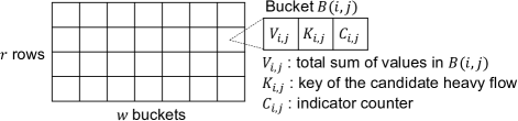
Figure 1: Data structure of MV-Sketch.

III-B Data Structure of MV-Sketch

Figure 1 shows the data structure of MV-Sketch, which is composed of a two-dimensional array of buckets with $r$ rows and $w$ columns. Let $B(i,j)$ denote the bucket at the $i$-th row and the $j$-th column, where $1\leq i\leq r$ and $1\leq j\leq w$. Each bucket $B(i,j)$ consists of three fields: (i) $V_{i,j}$, which counts the total sum of values of all flows hashed to the bucket; (ii) $K_{i,j}$, which tracks the key of the current candidate heavy flow in the bucket; and (iii) $C_{i,j}$, which is the indicator counter that checks if the candidate heavy flow should be kept or replaced as in MJRTY [12]. In addition, MV-Sketch is associated with $r$ pairwise-independent hash functions, denoted by $h_{1}\ldots h_{r}$, such that each $h_{i}$ (where $1\leq i\leq r$) hashes the key $x\in[n]$ of each incoming packet to one of the $w$ buckets in row $i$. Note that the data structure has a fixed memory size and can be pre-allocated in advance.

III-C Basic Operations

MV-Sketch supports two basic operations: (i) Update, which inserts each incoming packet into the sketch; (ii) Query, which returns the estimated sum of a given flow in an epoch.

Algorithm 1 shows the Update operation. All fields $V_{i,j}$, $K_{i,j}$, and $C_{i,j}$ are initialized as zero for $B(i,j)$, where $1\leq i\leq r$ and $1\leq j\leq w$. For each $(x,v_{x})$, we hash $x$ into $B(i,j)$ in the $i$-th row with $j=h_{i}(x)$ for $1\leq i\leq r$. We first increment $V_{i,j}$ by $v_{x}$ (Line 2). We then check if $x$ is stored in $K_{i,j}$ based on the MJRTY algorithm: if $K_{i,j}$ equals $x$, we increment $C_{i,j}$ by $v_{x}$ (Lines 3-4). Otherwise, we decrement $C_{i,j}$ by $v_{x}$ (Lines 5-6); if $C_{i,j}$ drops below zero, we replace $K_{i,j}$ by $x$ and reset $C_{i,j}$ with its absolute value (Lines 7-10). Note that the Update operation differs from MJRTY as it supports general value counts (or the number of bytes) with any non-negative value $v_{x}$, while MJRTY considers only vote counts (or the number of packets) with $v_{x}$ always being one.

Algorithm 1 Update

1:

2:for $i=1$ to $r$ do

3:    $V_{i,h_{i}(x)}\leftarrow V_{i,h_{i}(x)}+v_{x}$

4:    if $K_{i,h_{i}(x)}=x$ then

5:         $C_{i,h_{i}(x)}\leftarrow C_{i,h_{i}(x)}+v_{x}$

6:    else

7:         $C_{i,h_{i}(x)}\leftarrow C_{i,h_{i}(x)}-v_{x}$

8:         if $C_{i,h_{i}(x)}<0$ then

9:             $K_{i,h_{i}(x)}\leftarrow x$

10:             $C_{i,h_{i}(x)}\leftarrow-C_{i,h_{i}(x)}$

11:         end if

12:    end if

13:end for

Algorithm 2 shows the Query operation. For each hashed bucket in row $i$ (where $1\leq i\leq r$), we calculate a row estimate $\hat{S}_{i}(x)$ of flow $x$ (Lines 1-7): if $x$ and $K_{i,j}$ are the same, we set $\hat{S}_{i}(x)=(V_{i,j}+C_{i,j})/2$; otherwise, we set $\hat{S}_{i}(x)=(V_{i,j}-C_{i,j})/2$. The row estimate $\hat{S}_{i}(x)$ is actually the upper bound of $x$ in the hashed bucket $B(i,j)$ (Lemma 2). Finally, we return the final estimate $\hat{S}(x)$ as the minimum of all row estimates (Lines 8-9).

Algorithm 2 Query

1:

2:

3:for $i=1$ to $r$ do

4:    if $K_{i,h_{i}(x)}=x$ then

5:         $\hat{S}_{i}(x)\leftarrow(V_{i,h_{i}(x)}+C_{i,h_{i}(x)})/2$

6:    else

7:         $\hat{S}_{i}(x)\leftarrow(V_{i,h_{i}(x)}-C_{i,h_{i}(x)})/2$

8:    end if

9:end for

10:$\hat{S}(x)\leftarrow\min_{1\leq i\leq r}\{\hat{S}_{i}(x)\}$

11:return $\hat{S}(x)$

III-D Heavy Flow Detection

Heavy hitter detection. To detect heavy hitters, we check every bucket $B(i,j)$ ($1\leq i\leq r$ and $1\leq j\leq w$) at the end of an epoch. For each $B(i,j)$, if $V_{i,j}\geq\phi\mathcal{S}$, we let $x=K_{i,j}$ and query $\hat{S}(x)$ via Algorithm 2; if $\hat{S}(x)\geq\phi\mathcal{S}$, we report $x$ as a heavy hitter.

Heavy changer detection. To detect heavy changers, we compare two sketches at the ends of two epochs. One possible detection approach is to exploit the linear property of sketches as in prior studies [18, 33, 40], in which we compute the differences of $V_{i,j}$’s of the buckets at the same positions across the two sketches and recover the flows from the buckets whose differences exceed the threshold $\phi\mathcal{D}$ (Section II-A). However, such an approach can return many false negatives, since the hash collisions of two heavy changers, one with a high incremental change and another with a high decremental change, can cancel out the changes of each other.

To reduce the number of false negatives, we instead use the estimated maximum change of a flow for heavy changer detection. Specifically, let $U(x)$ and $L(x)$ be the upper and lower bounds of $S(x)$, respectively. We set $U(x)=\hat{S}(x)$ returned by Algorithm 2. Also, we set $L(x)=\max_{1\leq i\leq r}\{L_{i}(x)\}$, where $L_{i}(x)$ is set as follows: for each hashed bucket $B(i,j)$ of $x$ (where $1\leq i\leq r$ and $j=h_{i}(x)$), if $K_{i,j}$ equals $x$, we set $L_{i}(x)=C_{i,j}$; otherwise, we set $L_{i}(x)=0$. Note that both $U(x)$ and $L(x)$ are the true upper and lower bounds of $S(x)$, respectively (Lemma 2 in Section IV-B). Now, let $U^{1}(x)$ and $L^{1}(x)$ (resp. $U^{2}(x)$ and $L^{2}(x)$) be the upper and lower bounds of $S(x)$ in the previous (resp. current) epoch, respectively. Then the estimated maximum change of flow $x$ is given by $\hat{D}(x)=\max\{|U^{1}(x)-L^{2}(x)|,|L^{1}(x)-U^{2}(x)|\}$.

We now detect heavy changers as follows. We check every bucket $B(i,j)$ ($1\leq i\leq r$ and $1\leq j\leq w$) of two sketches of the previous and current epochs. For each $B(i,j)$ in each of the sketches, if $V_{i,j}\geq\phi\mathcal{D}$, we let $x=K_{i,j}$ and estimate $\hat{D}(x)$; if $\hat{D}(x)\geq\phi\mathcal{D}$, we report $x$ as a heavy changer (note that a necessary condition of a heavy changer is that its sum must exceed the threshold in at least one epoch).

Currently, MV-Sketch focuses on the values (e.g., packet or byte counts) of a flow. We can extend MV-Sketch to monitor hosts with a high number of distinct connections in DDoS or superspreader detection by either associating the buckets with approximate distinct counters [17] or filtering duplicate connections with a Bloom filter [50].

III-E Scalable Heavy Flow Detection

We can improve the performance and scalability of MV-Sketch by performing heavy flow detection on multiple packet streams in parallel based on a distributed streaming architecture [26]. Specifically, we deploy $q\geq 1$ detectors, each of which deploys an MV-Sketch instance to monitor packets from multiple streaming sources. Suppose that each streaming source maps a flow to a subset $d$ out of $q$ detectors, where $d\leq q$, and dispatches each packet of the flow uniformly to one of the $d$ selected detectors. At the end of each epoch, each detector sends the local detection results to a centralized controller for final heavy flow detection.

For heavy hitter detection, each detector checks every bucket $B(i,j)$ in MV-Sketch. Let $x=K_{i,j}$, and if $\hat{S}(x)\geq\tfrac{\phi}{d}\mathcal{S}$, the detector sends the tuple ($x$, $\hat{S}(x)$) of flow $x$ to the controller. After collecting all results from $q$ detectors, the controller adds the estimates of each flow. If the added estimate of a flow exceeds $\phi\mathcal{S}$, the flow is reported as a heavy hitter.

For heavy changer detection, each detector checks every bucket $B(i,j)$ of two sketches of the previous and current epochs. If $V_{i,j}\geq\tfrac{\phi}{d}\mathcal{D}$, it lets $x=K_{i,j}$ and estimates $\hat{D}(x)$; if $\hat{D}(x)\geq\tfrac{\phi}{d}\mathcal{D}$, the detector sends the tuple ($x$, $\hat{D}(x)$) of flow $x$ to the controller. The controller adds the estimates of each flow from $q$ detectors. If the added estimate of a flow exceeds $\phi\mathcal{D}$, the flow is reported as a heavy changer.

III-F Network-Wide Heavy Flow Detection

Algorithm 3 Merge

1:

2:

3:for $i=1$ to $r$ do

4:    for $j=1$ to $w$ do

5:         $V_{i,j}\leftarrow\sum_{1\leq k\leq q}V^{k}_{i,j}$

6:         $T\leftarrow\{K^{1}_{i,j},K^{2}_{i,j},\dots,K^{q}_{i,j}\}$

7:         for $x\in T$ do

8:             $e(x)\leftarrow 0$

9:             for $k=1$ to $q$ do

10:                 if $K^{k}_{i,j}=x$ then

11:                     $e(x)\leftarrow e(x)+(V^{k}_{i,j}+C^{k}_{i,j})/2$

12:                 else

13:                     $e(x)\leftarrow e(x)+(V^{k}_{i,j}-C^{k}_{i,j})/2$

14:                 end if

15:             end for

16:         end for

17:         $K_{i,j}\leftarrow x^{*}$, where $x^{*}=\operatorname*{arg\,max}_{x\in T}\{e(x)\}$

18:         $C_{i,j}\leftarrow\max\{2e(x^{*})-V_{i,j},0\}$

19:    end for

20:end for

We can also perform network-wide heavy-flow detection via MV-Sketch by deploying multiple MV-Sketch instances in multiple detectors (e.g., end-hosts or programmable switches) that span across the whole network and aggregating the measurement results from all detectors in a centralized controller, as in recent sketch-based network-wide measurement systems [48, 36, 34, 32, 25, 27, 46]. While scalable detection (Section III-E) focuses on improving scalability by processing multiple packet streams in parallel, network-wide detection aims to provide an accurate network-wide measurement view as if all traffic were measured in one big detector [34].

In network-wide heavy flow detection, we deploy an MV-Sketch instance in each of the detectors, such that all MV-Sketch instances share the same hash functions and parameter settings. We assume that each packet being monitored appears at only one MV-Sketch instance to avoid duplicate measurement (e.g., by monitoring only the ingress or egress traffic). We deploy a centralized controller that collects and merges the MV-Sketch instances from all detectors. Note that we do not make any assumption on the traffic size distribution of a heavy flow in each detector (e.g., a heavy flow may have small traffic size in some detectors); this is in contrast to scalable detection (Section III-E), in which we assume that the traffic size of a flow is uniformly distributed across detectors.

Algorithm 3 shows how the controller merges multiple MV-Sketch instances. Suppose that there are $q\geq 1$ detectors. Let $B^{k}(i,j)$ denote the bucket in the $i$-th row and $j$-th column of MV-Sketch in the $k$-th detector, where $1\leq i\leq r$, $1\leq j\leq w$, and $1\leq k\leq q$. Let $V^{k}_{i,j}$, $K^{k}_{i,j}$, and $C^{k}_{i,j}$ denote the total sum of values hashed to the bucket, the candidate heavy flow key, and the indicator counter of $B^{k}(i,j)$, respectively. Also, let $B(i,j)$ (with the corresponding fields $V_{i,j}$, $K_{i,j}$, and $C_{i,j}$) be the bucket in the $i$-th row and $j$-th column in the merged sketch. In Algorithm 3, the controller constructs each bucket $B(i,j)$ of the merged sketch by merging all $B^{k}(i,j)$ that have the same $i$ and $j$ in all $q$ detectors. The controller first sets $V_{i,j}$ as the sum of $V^{k}_{i,j}$’s of all $q$ detectors (Line 3). It then calculates a network-wide estimate $e(x)$ for each candidate heavy flow key $x\in T=\{K^{k}_{i,j}\}_{1\leq k\leq q}$ (note that $x$ is hashed to every bucket $B^{k}(i,j)$ for all $k$, where $1\leq k\leq q$). First, the controller initializes $e(x)$ as zero. For each $B^{k}(i,j)$ ($1\leq k\leq q$), if $K^{k}_{i,j}$ equals $x$, the controller increments $e(x)$ by $(V^{k}_{i,j}+C^{k}_{i,j})/2$; otherwise, it increments $e(x)$ by $(V^{k}_{i,j}-C^{k}_{i,j})/2$ (Lines 4-14). After that, the controller stores the key $x^{*}$ that has the maximum estimate among all candidate heavy flow keys into $K_{i,j}$ (Line 15). It also sets $C_{i,j}$ as the maximum value of $2e(x^{*})-V_{i,j}$ and zero (Line 16). By Lemma 2 in Section IV-B, we can show that the network-wide estimate $e(x)$ after Line 14 is an upper-bound of $S(x)$ (i.e., $e(x)\geq S(x)$).

Once the controller finishes the merge operation, it performs heavy flow detection on the merged MV-Sketch as in Section III-D. We show that the merged MV-Sketch achieves the same theoretical guarantee on accuracy as in a single MV-Sketch (Section IV-E).

IV Theoretical Analysis

We present theoretical analysis on MV-Sketch in heavy flow detection. We also compare MV-Sketch with several state-of-the-art invertible sketches.

IV-A Space and Time Complexities

Our analysis assumes that MV-Sketch is configured with $r=\log{\tfrac{1}{\delta}}$ and $w=\tfrac{2}{\epsilon}$, where $\epsilon$ ($0<\epsilon<1$) is the approximation parameter, $\delta$ ($0<\delta<1$) is the error probability, and the logarithm base is 2. Theorem 1 states the space and time complexities of MV-Sketch.

Theorem 1.

The space usage is $O(\tfrac{1}{\epsilon}\log{\tfrac{1}{\delta}}\log{n})$. The update time per packet is $O(\log\tfrac{1}{\delta})$, while the detection time of returning all heavy flows is $O(\tfrac{1}{\epsilon}\log^{2}\tfrac{1}{\delta})$.

Proof.

Each bucket of MV-Sketch stores a $\log{n}$-bit candidate heavy flow and two counters, so the space usage of MV-Sketch is $O(rw\log n)=O(\tfrac{1}{\epsilon}\log{\tfrac{1}{\delta}}\log{n})$.

Each per-packet update accesses $r$ buckets and requires $r=\log\tfrac{1}{\delta}$ hash operations, thereby taking $O(\log\tfrac{1}{\delta})$ time.

Returning all heavy flows requires to traverse all $rw$ buckets. For each bucket whose $V_{i,j}$ is above the threshold, we check $r$ buckets to obtain the estimate (either $\hat{S}(x)$ or $\hat{D}(x)$) for $x=K_{i,j}$. This takes $O(r^{2}w)=O(\tfrac{1}{\epsilon}\log^{2}\tfrac{1}{\delta})$ time. ∎

IV-B Error Bounds for Heavy Hitter Detection

Suppose that for all flows hashed to a bucket $B(i,j)$, flow $x$ is said to be a majority flow of $B(i,j)$ if its sum $S(x)$ is more than half of the total value count $V_{i,j}$. Then Lemma 1 states that the majority flow must be tracked; note that it is a generalization of the main result of MJRTY [12].

Lemma 1.

If there exists a majority flow $x$ in $B(i,j)$, then it must be stored in $K_{i,j}$ at the end of an epoch.

Proof.

We prove by contradiction. By definition, the majority flow $x$ has $S(x)>\tfrac{1}{2}V_{i,j}$. Suppose that $K_{i,j}\neq x$. Then the increments (resp. decrements) of $C_{i,j}$ due to $x$ must be offset by the decrements (resp. increments) of other flows that are also hashed to $B(i,j)$. This requires that $V_{i,j}-S(x)\geq S(x)$ (i.e., the total value count of other flows is larger than $S(x)$). Thus, $V_{i,j}\geq 2S(x)>V_{i,j}$, which is a contradiction. ∎

Lemma 2 next bounds the sum $S(x)$ of flow $x$.

Lemma 2.

Consider a bucket $B(i,j)$ that flow $x$ is hashed to. If $K_{i,j}$ equals $x$, then $C_{i,j}\leq S(x)\leq\tfrac{V_{i,j}+C_{i,j}}{2}$; otherwise, $0\leq S(x)\leq\tfrac{V_{i,j}-C_{i,j}}{2}$.

Proof.

Suppose that $K_{i,j}$ equals $x$. Let $\Delta$ be the offset amount of $x$ from $C_{i,j}$ due to other flows. Then we have $S(x)=C_{i,j}+\Delta\geq C_{i,j}$. Also, since $V_{i,j}\geq S(x)+\Delta=C_{i,j}+2\Delta$, we have $\Delta\leq\tfrac{V_{i,j}-C_{i,j}}{2}$. Thus, $S(x)=C_{i,j}+\Delta\leq\tfrac{V_{i,j}+C_{i,j}}{2}$.

Suppose now that $K_{i,j}\neq x$. Then the increments (resp. decrements) of $C_{i,j}$ due to $x$ must be offset by the decrements (resp. increments) made by other flows that are also hashed to the same bucket (see the proof of Lemma 1). The total value count of all flows other than $x$ (i.e., $V_{i,j}-S(x)$) minus the offset amount $S(x)$ is at least $C_{i,j}$. Thus, we have $V_{i,j}\geq C_{i,j}+2S(x)$, implying that $0\leq S(x)\leq\tfrac{V_{i,j}-C_{i,j}}{2}$. ∎

We now study the bounds of the estimated sum $\hat{S}(x)$ of flow $x$ returned by Algorithm 2. From Lemma 2 and the definition of $\hat{S}(x)$ in Algorithm 2, we see that $\hat{S}(x)\geq S(x)$. Also, Lemma 3 states the upper bound of $\hat{S}(x)$ in terms of $\epsilon$ and $\delta$.

Lemma 3.

$\hat{S}(x)\leq S(x)+\tfrac{\epsilon\mathcal{S}}{2}$ with a probability at least $1-\delta$.

Proof.

Consider the expectation of the total sum of all flows except $x$ in each bucket $B(i,j)$. It is given by $E[V_{i,j}-S(x)]=E[\textstyle\sum_{y\neq x,h_{i}(y)=h_{i}(x)}S(y)]\leq\tfrac{\mathcal{S}-S(x)}{w}\leq\tfrac{\epsilon\mathcal{S}}{2}$ due to the pairwise independence of $h_{i}$ and the linearity of expectation. By Markov’s inequality, we have

$$\Pr[V_{i,j}-S(x)\geq\epsilon\mathcal{S}]\leq\tfrac{1}{2}.$$ (1)

We now consider the row estimate $\hat{S}_{i}(x)$ (Algorithm 2). If $K_{i,j}$ equals $x$, then $\hat{S}_{i}(x)-S(x)=\tfrac{V_{i,j}+C_{i,j}}{2}-S(x)\leq\tfrac{V_{i,j}-S(x)}{2}$ due to Lemma 2; if $K_{i,j}\neq x$, then $\hat{S}_{i}(x)-S(x)=\tfrac{V_{i,j}-C_{i,j}}{2}-S(x)\leq\tfrac{V_{i,j}}{2}-S(x)\leq\tfrac{V_{i,j}-S(x)}{2}$.

Combining both cases, we have $\Pr[\hat{S}_{i}(x)-S(x)\geq\tfrac{\epsilon\mathcal{S}}{2}]\leq\Pr[\tfrac{V_{i,j}-S(x)}{2}\geq\tfrac{\epsilon\mathcal{S}}{2}]\leq\tfrac{1}{2}$ due to Equation (1).

Since $\hat{S}(x)$ is the minimum of all row estimates, we have $\Pr[\hat{S}(x)\leq S(x)+\tfrac{\epsilon\mathcal{S}}{2}]=1-\Pr[\hat{S}(x)-S(x)\geq\tfrac{\epsilon\mathcal{S}}{2}]=1-\Pr[\hat{S}_{i}(x)-S(x)\geq\tfrac{\epsilon\mathcal{S}}{2},\forall i]\geq 1-(\tfrac{1}{2})^{r}=1-\delta$. ∎

Theorem 2 summarizes the error bounds for heavy hitter detection in MV-Sketch.

Theorem 2.

MV-Sketch reports every heavy hitter with a probability at least $1-\delta$ (provided that $\phi\mathcal{S}\geq\epsilon\mathcal{S}$), and falsely reports a non-heavy hitter with sum no more than $(\phi-\tfrac{\epsilon}{2})\mathcal{S}$ with a probability at most $\delta$.

Proof.

We first prove that MV-Sketch reports each heavy hitter (say $x$) with a high probability. If flow $x$ is the majority flow in any one of its hashed buckets, it will be reported due to Lemma 1. MV-Sketch fails to report $x$ only if $x$ is not the majority flow of any of its $r$ hashed buckets, i.e., $S(x)\leq\tfrac{V_{i,j}}{2}$ for $1\leq i\leq r$ and $j=h_{i}(x)$. The probability that it occurs (denoted by $P$) is $P=\Pr[S(x)\leq\tfrac{V_{i,j}}{2},\forall i]=\Pr[V_{i,j}-S(x)\geq S(x),\forall i]$. Since $S(x)\geq\phi\mathcal{S}\geq\epsilon\mathcal{S}$, we have $P\leq\Pr[V_{i,j}-S(x)\geq\epsilon\mathcal{S},\forall i]\leq(\tfrac{1}{2})^{r}=\delta$ due to Equation (1). Thus, a heavy hitter is reported with a probability at least $1-\delta$.

We next prove that MV-Sketch reports a non-heavy hitter (say $y$) with $S(y)\leq(\phi-\tfrac{\epsilon}{2})\mathcal{S}$ with a small probability. A necessary condition is that $y$ has its estimate $\hat{S}(y)\geq\phi\mathcal{S}$. Thus, $\hat{S}(y)-S(y)\geq\phi\mathcal{S}-(\phi-\tfrac{\epsilon}{2})S=\tfrac{\epsilon\mathcal{S}}{2}$. From Lemma 3, we have $\Pr[\hat{S}(y)-S(y)\geq\tfrac{\epsilon\mathcal{S}}{2}]\leq\delta$. In other words, $y$ is reported as a heavy hitter with a probability at most $\delta$. ∎

TABLE I: Comparison of MV-Sketch with state-of-the-art invertible sketches.

Sketch	$r$	$w$	FN Prob.	Space	Update time	Detection time
Count-Min-Heap	$\log{\tfrac{1}{\delta}}$	$\tfrac{2}{\epsilon}$	0	$O(\tfrac{1}{\epsilon}\log{\tfrac{1}{\delta}}+H\log{n})$	$O(\log{\tfrac{H}{\delta}})$	$O(H)$
LD-Sketch	$\log{\tfrac{1}{\delta}}$	$\tfrac{2H}{\epsilon}$	0	$O(\frac{H}{\epsilon}\log{\tfrac{1}{\delta}}\log{n})$	$O(\log{\tfrac{1}{\delta}})$	$O(\frac{H}{\epsilon}\log{\frac{1}{\delta}})$
Deltoid	$\log{\tfrac{1}{\delta}}$	$\tfrac{2}{\epsilon}$	$\delta$	$O(\frac{1}{\epsilon}\log{\tfrac{1}{\delta}}\log{n})$	$O(\log\tfrac{1}{\delta}\log{n})$	$O(\frac{1}{\epsilon}\log^{2}{\tfrac{1}{\delta}}\log{n})$
Fast Sketch	$4H\log{\tfrac{4}{\delta}}$	$1\!+\!\log\tfrac{n}{4H\log{(4/\delta)}}$	$\delta$	$O(H\log{\tfrac{1}{\delta}}\log\tfrac{n}{H\log(1/\delta)})$	$O(\log{\tfrac{1}{\delta}}\log\tfrac{n}{H\log{(1/\delta)}})$	$O(H\log^{3}{\tfrac{1}{\delta}}\log(\tfrac{n}{H\log{(1/\delta)}}))$
MV-Sketch	$\log{\tfrac{1}{\delta}}$	$\tfrac{2}{\epsilon}$	$\delta$	$O(\frac{1}{\epsilon}\log{\tfrac{1}{\delta}}\log{n})$	$O(\log{\tfrac{1}{\delta}})$	$O(\frac{1}{\epsilon}\log^{2}{\tfrac{1}{\delta}})$

IV-C Error Bounds for Heavy Changer Detection

Recall that heavy changer detection relies on the upper bound $U(x)$ and the lower bound $L(x)$ of $S(x)$ (Section III-D). From Lemma 2, both $U(x)$ and $L(x)$ are the true upper and lower bounds of $S(x)$, respectively. Lemma 3 has shown that $U(x)$, which equals $\hat{S}(x)$, differs from $S(x)$ by a small range with a high probability. Now, Lemma 4 shows that $L(x)$ and $S(x)$ also differ by a small range with a high probability.

Lemma 4.

$S(x)-L(x)\leq\epsilon\mathcal{S}$ with a probability at least $1-\delta$.

Proof.

Consider the lower bound estimate $L_{i}(x)$ given by the hashed bucket $B(i,j)$ of flow $x$ (where $1\leq i\leq r$) (Section III-D). If $K_{i,j}$ equals $x$, $L_{i}(x)=C_{i,j}$. By Lemma 2, we have $S(x)\leq\tfrac{V_{i,j}+C_{i,j}}{2}$, implying that $S(x)-L_{i}(x)=S(x)-C_{i,j}\leq V_{i,j}-S(x)$.

If $K_{i,j}\neq x$, $L_{i}=0$ and $x$ is not the majority flow for bucket $B(i,j)$. We have $S(x)-L_{i}(x)=S(x)\leq V_{i,j}-S(x)$.

Combining both cases, we have $\Pr[S(x)-L(x)\geq\epsilon\mathcal{S}]=\Pr[S(x)-L_{i}(x)\geq\epsilon\mathcal{S},\forall i]\leq\Pr[V_{i,j}-S(x)\geq\epsilon\mathcal{S},\forall i]\leq(\tfrac{1}{2})^{r}=\delta$ due to Equation (1). ∎

Lemma 5 provides an upper bound of the estimated maximum change $\hat{D}(x)=\max\{|U^{1}(x)-L^{2}(x)|,|U^{2}(x)-L^{1}(x)|\}$ in terms of $\mathcal{S}^{1}$ and $\mathcal{S}^{2}$, which are the total sums of all flows in the previous and current epochs, respectively.

Lemma 5.

$\hat{D}(x)\leq D(x)+\epsilon(\mathcal{S}^{1}+\mathcal{S}^{2})$ with a probability at least $(1-\delta)^{2}$.

Proof.

Without loss of generality, we consider $\hat{D}(x)=|U^{1}(x)-L^{2}(x)|$. Let $S^{1}(x)$ and $S^{2}(x)$ be the sums of $x$ in the previous and current epochs, respectively. Let $e_{u}^{1}(x)=U^{1}(x)-S^{1}(x)$ and $e_{l}^{2}=S^{2}(x)-L^{2}(x)$. Then $\hat{D}(x)=|S^{1}(x)+e_{u}^{1}(x)-(S^{2}(x)-e_{l}^{2}(x))|\leq D(x)+e_{u}^{1}(x)+e_{l}^{2}(x)$. Since $e_{u}^{1}(x)$ and $e_{l}^{2}(x)$ are independent, we have $\Pr[e_{u}^{1}(x)+e_{l}^{2}(x)\leq\epsilon(\mathcal{S}^{1}+\mathcal{S}^{2})]\geq\Pr[e_{u}^{1}(x)\leq\epsilon\mathcal{S}^{1}]\cdot\Pr[e_{l}^{2}(x)\leq\epsilon\mathcal{S}^{2}]\geq(1-\delta)^{2}$, where the last inequality is due to Lemmas 3 and 4. Thus, $\Pr[\hat{D}(x)-D(x)\leq\epsilon(\mathcal{S}^{1}+\mathcal{S}^{2})]\geq\Pr[e_{u}^{1}(x)+e_{l}^{2}(x)\leq\epsilon(\mathcal{S}^{1}+\mathcal{S}^{2})]\geq(1-\delta)^{2}$. ∎

Theorem 3 summarizes the error bounds for heavy changer detection in MV-Sketch.

Theorem 3.

MV-Sketch reports every heavy changer with a probability at least $1-\delta$ (provided that $\tfrac{\phi\mathcal{D}}{\epsilon}\geq\max\{\mathcal{S}^{1},\mathcal{S}^{2}\}$), and falsely reports any non-heavy changer with change no more than $\phi\mathcal{D}-\epsilon(\mathcal{S}^{1}+\mathcal{S}^{2})$ with a probability at most $1-(1-\delta)^{2}$.

Proof.

We first prove that MV-Sketch reports each heavy changer (say $x$) with a high probability. If flow $x$ is the majority flow in any one of its hashed buckets, it must be reported, as its estimate $\hat{D}(x)\geq D(x)\geq\phi\mathcal{D}$. Flow $x$ is not reported only if it is not stored as a candidate heavy flow in both sketches. Since there must exist one sketch (either in the previous or current epoch) with $S(x)\geq\phi\mathcal{D}$, by Theorem 2, the probability that $x$ is not reported in that sketch is at most $\delta$ (assuming that $\tfrac{\phi\mathcal{D}}{\epsilon}\geq\max\{\mathcal{S}^{1},\mathcal{S}^{2}\}$). Thus, a heavy changer is reported with a probability at least $1-\delta$.

We next prove that MV-Sketch reports a non-heavy changer (say $y$) with $D(y)\leq\phi\mathcal{D}-\epsilon(\mathcal{S}^{1}+\mathcal{S}^{2})$ with a small probability. Let $\hat{D}(y)=D(y)+\Delta$ for some $\Delta$; hence, $\hat{D}(y)\leq\phi\mathcal{D}-\epsilon(\mathcal{S}^{1}+\mathcal{S}^{2})+\Delta$. If $y$ is reported as a heavy changer, it requires that $\Delta\geq\epsilon(\mathcal{S}^{1}+\mathcal{S}^{2})$ and such a probability is at most $1-(1-\delta)^{2}$ due to Lemma 5. ∎

IV-D Error Bounds for Scalable Heavy Flow Detection

We generalize the analysis for a single detector in Theorems 2 and 3 for scalable heavy flow detection under MV-Sketch. Our analysis assumes that the stream of packets of each flow is uniformly distributed to $d\leq q$ detectors.

Theorem 4.

The controller reports every heavy hitter with a probability at least $(1-\delta)^{d}$, and falsely reports a non-heavy hitter with sum no more than $\tfrac{d}{q}(\phi-\tfrac{\epsilon}{2})\mathcal{S}$ with a probability at most $1-(1-\delta)^{d}$.

Proof.

We first study the probability of reporting each heavy hitter (say $x$). Recall that the estimate of $x$ at each detector is at least $\frac{\phi}{d}\mathcal{S}$ (Section IV-B). If all $d$ detectors report flow $x$ to the controller, flow $x$ must be reported as a heavy hitter since its added estimate is at least $d\times\frac{\phi}{d}\mathcal{S}=\phi\mathcal{S}$. Such a probability is at least $(1-\delta)^{d}$ by Theorem 2.

We next study the probability of reporting a non-heavy hitter (say $y$). It happens if at least one detector reports flow $y$ to the controller. If $S(y)\leq\tfrac{d}{q}(\phi-\tfrac{\epsilon}{2})\mathcal{S}$, the sum of flow $y$ at each detector is at most $\tfrac{1}{q}(\phi-\tfrac{\epsilon}{2})\mathcal{S}$. From Theorem 2, the probability that a detector reports flow $y$ is at most $\delta$. Thus, it is falsely reported as a heavy hitter by the controller with a probability at most $1-(1-\delta)^{d}$. ∎

Theorem 5.

The controller reports every heavy changer with a probability at least $(1-\delta)^{d}$, and falsely reports a non-heavy changer with change no more than $\tfrac{d}{q}(\phi\mathcal{D}-\epsilon(\mathcal{S}^{1}+\mathcal{S}^{2}))$ with a probability at most $1-(1-\delta)^{2d}$.

Proof.

It is similar to that in Theorem 4 and omitted. ∎

IV-E Error Bounds for Network-Wide Heavy Flow Detection

For network-wide heavy flow detection, we can readily check that the complexity of the merge operation in Algorithm 3 is $O(rwq^{2})=O(\tfrac{q^{2}}{\epsilon}\log{\tfrac{1}{\delta}})$. In the following, we analyze the error bounds for network-wide heavy flow detection.

Lemma 6 shows that if there exists a majority flow (defined in Section IV-B) in a bucket of the merged sketch, then the bucket can track the majority flow, even though each of the detectors only sees a portion of traffic of the majority flow.

Lemma 6.

After the $q$ MV-Sketch instances are merged, if there exists a majority flow $x$ in $B(i,j)$ in the merged sketch, then it must be stored in $K_{i,j}$.

Proof.

We first show that $x$ is stored in $K^{k}_{i,j}$ in at least one $B^{k}(i,j)$ for $1\leq k\leq q$. Suppose that the contrary holds. Then by Lemma 2, $S(x)\leq\sum_{k}\tfrac{V^{k}_{i,j}-C^{k}_{i,j}}{2}\leq\tfrac{V_{i,j}}{2}$, which contradicts the definition of a majority flow.

We next show that $x$ must be the key with the maximum network-wide estimate among all $K^{k}_{i,j}$’s for $1\leq k\leq q$. Suppose the contrary that $y\neq x$ is the maximum key being returned. Without loss of generality, let $K_{i,j}^{k}=x$ for $1\leq k\leq t$ for some $t\geq 1$. By Algorithm 3, the network-wide estimates of $x$ and $y$ are $e(x)=\textstyle\sum_{1\leq k\leq t}\!\tfrac{V^{k}_{i,j}+C^{k}_{i,j}}{2}+\textstyle\sum_{t+1\leq k\leq q}\!\tfrac{V^{k}_{i,j}-C^{k}_{i,j}}{2}$ and $e(y)\leq$ $\textstyle\sum_{1\leq k\leq t}\!\tfrac{V^{k}_{i,j}-C^{k}_{i,j}}{2}+\textstyle\sum_{t+1\leq k\leq q}\!\tfrac{V^{k}_{i,j}+C^{k}_{i,j}}{2}$, respectively. Thus, $e(x)+e(y)\leq\sum_{k}V^{k}_{i,j}=V_{i,j}$.

This implies that $V_{i,j}\geq 2e(x)$ as $y$ is the maximum key. By Lemma 2, $e(x)$ is an upper bound of $S(x)$, but $2S(x)>V_{i,j}$ as $x$ is a majority flow. This leads to a contradiction. ∎

Lemma 7 bounds the sum $S(x)$ of flow $x$ in the merged sketch, where $S(x)$ now corresponds to the network-wide sum.

Lemma 7.

Consider a bucket $B(i,j)$ that flow $x$ is hashed to in the merged sketch. If $K_{i,j}$ equals $x$, then $C_{i,j}\leq S(x)\leq\tfrac{V_{i,j}+C_{i,j}}{2}$; otherwise, $0\leq S(x)\leq\tfrac{V_{i,j}-C_{i,j}}{2}.$

Proof.

Suppose $K_{i,j}\!=\!x$. Without loss of generality, let $K_{i,j}^{k}=x$ for $1\!\leq\!k\!\leq\!t$ for some $t\!\geq\!1$. By Algorithm 3, $2e(x)-V_{i,j}\!=\!2(\textstyle\sum_{1\leq k\leq t}\!\tfrac{V^{k}_{i,j}+C^{k}_{i,j}}{2}$ $+\textstyle\sum_{t+1\leq k\leq q}\!\tfrac{V^{k}_{i,j}\!-\!C^{k}_{i,j}}{2})-V_{i,j}\!=\!\textstyle\sum_{1\leq k\leq t}C^{k}_{i,j}$ $-\textstyle\sum_{t+1\leq k\leq q}C^{k}_{i,j}$ $\leq\textstyle\sum_{1\leq k\leq t}C^{k}_{i,j}\leq S(x)$ (the last inequality is due to Lemma 2). Thus, $C_{i,j}=\max\{2e(x)-V_{i,j},0\}\leq S(x)$.

Also, by Lemma 2, $e(x)\geq S(x)$. Since $V_{i,j}$ is the total sum of values in $B(i,j)$, $V_{i,j}\geq S(x)$. Thus, $\tfrac{V_{i,j}+C_{i,j}}{2}\geq\tfrac{V_{i,j}+2e(x)-V_{i,j}}{2}=e(x)\geq S(x)$.

Suppose now $K_{i,j}\neq x$. Let $K_{i,j}=y$, meaning that $e(y)$ is the maximum network-wide estimate among all keys hashed to $B(i,j)$. Without loss of generality, let $K_{i,j}^{k}=y$ for $1\!\leq\!k\!\leq\!t$ for some $t\!\geq\!1$. Note that $C_{i,j}=\max\{2e(y)-V_{i,j},0\}$. If $C_{i,j}=0$, then $2e(y)-V_{i,j}\leq 0$. Thus, $S(x)\leq e(x)\leq e(y)\leq\tfrac{V_{i,j}}{2}=\tfrac{V_{i,j}-C_{i,j}}{2}$.

If $C_{i,j}\neq 0$, then $\tfrac{V_{i,j}-C_{i,j}}{2}\!=\!V_{i,j}\!-\!e(y)\!=\!\textstyle\sum_{k}\!V^{k}_{i,j}-\textstyle\sum_{1\leq k\leq t}\!\tfrac{V^{k}_{i,j}+C^{k}_{i,j}}{2}$ $-\textstyle\sum_{t+1\leq k\leq q}\!\tfrac{V^{k}_{i,j}-C^{k}_{i,j}}{2}$ $=\textstyle\sum_{1\leq k\leq t}\!\tfrac{V^{k}_{i,j}-C^{k}_{i,j}}{2}$ $+\textstyle\sum_{t+1\leq k\leq q}\!\tfrac{V^{k}_{i,j}+C^{k}_{i,j}}{2}\geq S(x)$ (by Lemma 2). ∎

Theorem 6 summarizes the error bounds for network-wide heavy hitter and heavy changer detection in the merged MV-Sketch.

Theorem 6.

The merged MV-Sketch reports every heavy hitter with a probability at least $1-\delta$ (provided that $\phi\mathcal{S}\geq\epsilon\mathcal{S}$), and falsely reports a non-heavy hitter with sum no more than $(\phi-\tfrac{\epsilon}{2})\mathcal{S}$ with a probability at most $\delta$; it reports every heavy changer with a probability at least $1-\delta$ (provided that $\tfrac{\phi\mathcal{D}}{\epsilon}\geq\max\{\mathcal{S}^{1},\mathcal{S}^{2}\}$), and falsely reports any non-heavy changer with change no more than $\phi\mathcal{D}-\epsilon(\mathcal{S}^{1}+\mathcal{S}^{2})$ with a probability at most $1-(1-\delta)^{2}$.

Proof.

By Lemmas 6 and 7, the bounds of $S(x)$ in the merged MV-Sketch are the same as if all traffic were processed by a single MV-Sketch. Thus, the network-wide detection of MV-Sketch achieves the same accuracy as in local detection. ∎

IV-F Comparison with State-of-the-art Invertible Sketches

We present a comparative analysis on MV-Sketch and state-of-the-art invertible sketches, including Count-Min-Heap [16], LD-Sketch [26], Deltoid [18], and Fast Sketch [33]. In the interest of space, we focus on heavy hitter detection using a single sketch. Table I shows the false negative probability, and the space and time complexities, in terms of $\epsilon$, $\delta$, $n$, and $H$ (the maximum number of heavy hitters in an epoch).

We first study the false negative probability (i.e, the maximum probability of not reporting a heavy hitter); we study other accuracy metrics in Section VI. Both Count-Min-Heap and LD-Sketch guarantee zero false negatives as they are configured to keep all heavy hitters in extra structures, while MV-Sketch can miss a heavy hitter with a probability at most $\delta$. Nevertheless, MV-Sketch achieves almost zero false negatives in our evaluation based on real traces (Section VI).

Regarding the space complexity, all sketches have a $\log n$ term. However, it refers to $\log n$ bits (i.e., the key length) in Count-Min-Heap, LD-Sketch, and MV-Sketch, while it refers to $\log n$ integer counters in Deltoid and Fast Sketch.

Regarding the (per-packet) update time complexity, Count-Min-Heap updates the sketch ($O(\log\tfrac{1}{\delta})$ time) and accesses its heap if the packet is from a heavy flow ($O(\log H)$ time), and its update time increases with $H$. Both Deltoid and Fast Sketch have high time complexities, which increase with the key length $\log n$. Both MV-Sketch and LD-Sketch have the same update time complexities, yet LD-Sketch may need to expand its associative arrays on-the-fly and this decreases the overall throughput from our evaluation (Section VI).

We also present the detection time complexity. However, our evaluation shows that the detection time of recovering all heavy flows is very small (within milliseconds) for all sketches shown in Table I.

V Implementation in Programmable Switches

We study how to deploy MV-Sketch in programmable switches to support heavy flow detection in the data plane. However, realizing MV-Sketch with high performance in programmable switches is non-trivial, due to various restrictions in the switch programming model. In this section, we introduce PISA (Protocol-Independent Switch Architecture), and discuss the challenges of realizing MV-Sketch in PISA switches. Finally, we show how we overcome the challenges to make MV-Sketch deployable.

V-A Basics

We target a family of programmable switches based on PISA [11, 41]. A PISA switch consists of a programmable parser, followed by an ingress/egress pipeline of stages, and finally a de-parser. Packets are first parsed by the parser, which extracts header fields and custom metadata to form a packet header vector (PHV). The PHV is then passed to the ingress/egress pipeline of stages that comprises match-action tables. Each stage matches some fields of the PHV with a list of entries and applies a matched action (e.g., modifying PHV fields, updating persistent states, or performing routing) to the packet. Finally, the de-parser reassembles the modified PHV with the original packet and sends the packet to an output port. PISA switches are fast in packet forwarding, by limiting the complexity of stages in the pipeline. Each stage has its own dedicated resources, including SRAM and multiple arithmetic logic units (ALUs) that run in parallel.

PISA switches achieve programmability by supporting multiple customizable match-action tables in the same stage and connecting many stages into a pipeline. Programmers can write a program using a domain-specific language (e.g., P4 [10]) to define packet formats, build custom processing pipelines, and configure the match-action tables.

V-B Challenges

Supporting heavy flow detection in PISA switches must address the hardware resource constraints [39, 43, 23]: (i) the SRAM of each stage is of small and identical size (e.g., few megabytes); (ii) the number of available ALUs per stage is limited; (iii) the pipeline contains a fixed number of physical stages (e.g., 1-32); and (iv) only a limited size of a PHV can be passed across stages (e.g., few kilobits). Nevertheless, the small and static memory design feature of MV-Sketch makes it a good fit to address the limited resources in PISA switches.

However, realizing MV-Sketch in PISA switches still faces programming challenges, due to the restrictions in the switch programming model. Consider the update operation of MV-Sketch in Algorithm 1. For simplicity, we focus on $r=1$ row in the sketch in the following discussion, yet we can generalize our analysis for multiple rows by duplicating the single-row implementation. Intuitively, we can create three register arrays, namely $V$, $K$ and $C$, to track the total sum, the candidate flow key, and the indicator counter in MV-Sketch, respectively. However, there are several programming challenges.

Challenge 1 (C1): Limited computation capability for handling flow keys with more than 32 bits. ALUs of PISA switches now only support primitive arithmetic (e.g., addition and subtraction) on the variables of up to 32 bits. While MV-Sketch is also designed based on primitive arithmetic only, updating the candidate flow key in $K$ is beyond the capability of the ALUs since the size of a flow key is typically more than 32 bits (e.g., a 5-tuple flow key has 104 bits).

Challenge 2 (C2): Limited memory access for managing dependent fields. PISA switches support a limited memory access model. First, the time budget for each memory access is limited, as only one read-modify-write is allowed for each variable. Also, each memory block can only be accessed in the stage to which it belongs, meaning that we can only access a memory region once as a packet traverses the pipeline. Note that PISA switches allow concurrent memory accesses to mutually exclusive memory blocks in a single stage. However, in Algorithm 1, the operations on $K$ and $C$ are dependent on each other: the write to $C$ is conditioned on $K$ (Line 4), while the write to $K$ is conditioned on $C$ (Line 8). If we want to update $K$ and $C$ in one stage, we need to perform multiple reads and writes sequentially, which breaks the time budget of a stage; however, if we place $K$ and $C$ in different stages, $K$ needs to be accessed twice (the first access is to check the content of $K$ in Line 3, and the second access is to update $K$ in Line 8).

Challenge 3 (C3): Limited branching for updates. To simplify processing, PISA switches design their ALUs with a small circuit depth (e.g., 3) that hinders complicated predicted operations. The packet processing in a stage typically supports an if-else chain with at most two levels [41]. In Algorithm 1, updating $C$ requires a three-level if-else chain (Lines 4, 6, and 9), which makes it difficult to perform the update operation within one stage. While complex branching is allowed across stages, updating $C$ in different stages is infeasible with the memory access model of PISA switches (C2).

V-C Implementation

Algorithm 4 Implementation for 5-tuple flow keys

1:if Metadata.repass = 0 then

2:    // Stage 1: update $V_{h(x)}$ and access $(K^{1}_{h(x)},K^{2}_{h(x)})$

3:    $V_{h(x)}\leftarrow V_{h(x)}+v_{x}$

4:    if $(K^{1}_{h(x)},K^{2}_{h(x)})\neq(x_{1},x_{2})$ then

5:         Metadata.flag $\leftarrow$ 1

6:    end if

7:    // Stage 2: access $(K^{3}_{h(x)},K^{4}_{h(x)})$

8:    if $(K^{3}_{h(x)},K^{4}_{h(x)})\neq(x_{3},x_{4})$ then

9:         Metadata.flag $\leftarrow$ 1

10:    end if

11:    // Stage 3: update $C_{h(x)}$

12:    if Metadata.flag $\neq 1$  then

13:         $C_{h(x)}\leftarrow C_{h(x)}+v_{x}$

14:    else if Metadata.flag $=1$ and $C_{h(x)}\geq v_{x}$ then

15:         $C_{h(x)}\leftarrow C_{h(x)}-v_{x}$

16:    end if

17:    if Metadata.flag $=1$ and $C_{h(x)}<v_{x}$ then

18:         Metadata.repass $\leftarrow$ 1

19:    end if

20:    // Stage 4: recirculate $x$

21:    if Metadata.repass $=1$ then

22:         recirculate $x$

23:    end if

24:else

25:    // Stage 1: update $(K^{1}_{h(x)},K^{2}_{h(x)})$

26:    $(K^{1}_{h(x)},K^{2}_{h(x)})\leftarrow(x_{1},x_{2})$

27:    // Stage 2: update $(K^{3}_{h(x)},K^{4}_{h(x)})$

28:    $(K^{3}_{h(x)},K^{4}_{h(x)})\leftarrow(x_{3},x_{4})$

29:    // Stage 3: update $C$

30:    $C_{h(x)}\leftarrow v_{x}-C_{h(x)}$

31:end if

We elaborate how we address the challenges of implementing MV-Sketch in PISA switches. To address Challenge C1, we split a long flow key into multiple sub-keys and use multiple stages and ALUs to process the sub-keys. For example, we can split a 104-bit 5-tuple flow key into three 32-bit sub-keys and one 8-bit sub-key, and access each sub-key in one stage with a single ALU. To reduce the number of stages, we can use paired atoms [41] (an atom refers to a packet-processing unit) to update a pair of sub-keys in one stage. Specifically, in paired updates, the ALUs of PISA switches can read two 32-bit elements from the register memory, set up conditional branching based on both elements, perform primitive arithmetic, and write back the final results.

To address Challenges C2 and C3, we leverage the recirculation feature [43, 7] of PISA switches to eliminate the inter-dependency between $K$ and $C$ and the complex branching for updating $C$. We define the change point as the point where we need to update the candidate heavy flow key and negate the indicator counter during the update process (i.e., Lines 8-9 in Algorithm 1). Our idea is to put the operations at the change point in the second pass of a packet, such that the operations are carried out if and only if the packet is recirculated to the second pass of the switch pipeline. More concretely, in the first pass, we just read $K$, update $C$, and recirculate the packet if the change point appears; in the second pass, we update $K$ and negate $C$.

Algorithm 4 shows the pseudo-code of implementing MV-Sketch in PISA switches for 5-tuple flow keys. Let $V_{h(x)}$, $K_{h(x)}$, and $C_{h(x)}$ be the entries that $x$ is hashed into in the register arrays $V$, $K$, and $C$ via the hash function $h$, respectively. We split a 104-bit flow key $x$ into four sub-keys: source IP $x_{1}$, destination IP $x_{2}$, source-destination ports $x_{3}$, and protocol $x_{4}$. We use two register arrays, $(K^{1},K^{2})$ and $(K^{3},K^{4})$, to track the candidate heavy flow sub-keys, such that each element in the arrays is a pair of 32-bit variables. We use the metadata Metadata.repass, initialized as zero, in the first pass of each packet to control the execution of the pipeline. In the first pass of $x$, we perform the following operations. In Stage 1 and Stage 2, we update $V_{h(x)}$ and compare each sub-key with the candidate heavy flow sub-keys; if either sub-key is not matched, we set Metadata.flag as one (Lines 4-10). We update $C_{h(x)}$ based on the value of Metadata.flag in Stage 3 (Lines 11-16). Finally, in Stage 4, we check the value of Metadata.repass; if it is one, we recirculate the packet together with Metadata.repass to the switch pipeline (Lines 21-23). In the second pass of $x$, we update the two register arrays $(K^{1},K^{2})$ and $(K^{3},K^{4})$, as well as $C_{h(x)}$ (Lines 25-30).

Note that our evaluation (Section VI-B) shows that MV-Sketch requires a second pass only on a small fraction of packets (e.g., less than 5%), meaning that the recirculation overhead is limited.

V-D Optimizations

Algorithm 5 Size counting on 32-bit flow keys

1:if Metadata.repass = 0 then

2:    // Stage 1: update $V_{h(x)}$ and $(K_{h(x)},C_{h(x)})$

3:    $V_{h(x)}\leftarrow V_{h(x)}+v_{x}$

4:    if $K_{h(x)}=x$ then

5:         $C_{h(x)}\leftarrow C_{h(x)}+v_{x}$

6:    else if $K_{h(x)}\neq x$ and $C_{h(x)}\geq v_{x}$ then

7:         $C_{h(x)}\leftarrow C_{h(x)}-v_{x}$

8:    end if

9:    if $K_{h(x)}\neq x$ and $C_{h(x)}<v_{x}$ then

10:         $K_{h(x)}\leftarrow x$

11:         Metadata.repass = 1

12:    end if

13:    // Stage 2: recirculate $x$

14:    if Metadata.repass = 1 then

15:         recirculate $x$

16:    end if

17:else

18:    // Stage 1: this is the second pass

19:    $C_{h(x)}\leftarrow v_{x}-C_{h(x)}$

20:end if

Algorithm 6 Packet counting on 32-bit flow keys

1:// Stage 1: update $V_{h(x)}$ and $(K_{h(x)},C_{h(x)})$

2:$V_{h(x)}\leftarrow V_{h(x)}+v_{x}$

3:if $K_{h(x)}=x$ or $C_{h(x)}=0$ then

4:    $C_{h(x)}\leftarrow C_{h(x)}+1$

5:else

6:    $C_{h(x)}\leftarrow C_{h(x)}-1$

7:end if

8:if $K_{h(x)}\neq x$ and $C_{h(x)}=0$ then

9:    $K_{h(x)}\leftarrow x$

10:end if

We can optimize the implementation of MV-Sketch if the flow keys have no more than 32 bits (e.g, the source or destination IPv4 address). This allows us to access a flow key via a single ALU (i.e., C1 addressed), and update $K$ and $C$ atomically via paired atoms to address their dependency (i.e., C2 addressed). Specifically, we can place $K$ and $C$ in a 64-bit register array, in which the high 32 bits of each entry store the key field, while the low 32 bits store the indicator counter field. The paired atom packs the operations of reading, conditional branching, primitive arithmetic, and writing for both $K$ and $C$ atomically.

We show how to update the pair ($K$, $C$) via limited branching in two cases: (i) size counting, which counts the total bytes of each flow; and (ii) packet counting, which counts the number of packets of each flow. For size counting, similar to Algorithm 4, we put the update of $C$ at the change point in the second pass of the packet. For packet counting, the size $v_{x}$ of flow $x$ is the constant one. We observe that when the packet processing reaches the change point, the state of $C_{h(x)}$ is zero and should change from zero to one (Lines 6-9 in Algorithm 1). It is equivalent to incrementing $C_{h(x)}$ by one as in the case when $K_{h(x)}$ equals $x$ (Line 4 in Algorithm 1). By merging these two branches, we can change and reorganize the if-conditions in Algorithm 1 to reduce the three-level if-else chain to a two-level one, as well as eliminate the recirculation operations (i.e., C3 addressed).

Algorithms 5 and 6 summarize our optimized implementation of MV-Sketch for size counting and packet counting in PISA switches, respectively. Note that Lines 4-12 of Algorithm 5 and Lines 3-10 of Algorithm 6 can be done in one paired atom.

VI Evaluation

We conduct evaluation in both software and hardware environments. Our trace-driven evaluation in software shows that MV-Sketch achieves (i) high accuracy in heavy flow detection with small and static memory space, (ii) high processing speed, and (iii) high accuracy in scalable detection, compared to state-of-the-art invertible sketches. We also show how SIMD instructions can further boost the update performance of MV-Sketch in software. Furthermore, our evaluation in a Barefoot Tofino switch [45] shows that MV-Sketch achieves (i) line speed for packet counting and incurs slight (e.g., less than 5%) performance degradation for size counting, and (ii) incurs only limited switch resource overhead.

VI-A Evaluation in Software

Simulation testbed. We conduct our evaluation on a server equipped with an eight-core Intel Xeon E5-1630 3.70 GHz CPU and 16 GB RAM. The CPU has 64 KB of L1 cache per core, 256 KB of L2 cache per core, and 10 MB of shared L3 cache. The server runs Ubuntu 14.04.5. To exclude the I/O overhead on performance, we load all datasets into memory prior to all experiments.

Dataset. We use the anonymized Internet traces from CAIDA [14], captured on an OC-192 backbone link in April 2016. The original traces are one hour long, and we focus on the first five minutes of the traces in our evaluation. We divide the traces into five one-minute epochs and obtain the average results. We measure IPv4 packets only. Each epoch contains 29 M packets, 1 M flows, and 6 M unique IPv4 addresses on average.

Methodology. We take the source/destination address pairs as flow keys (64 bits long). For evaluation purposes, we generate the ground truths by finding $\mathcal{S}$ and $\mathcal{D}$, and hence the true heavy flows, for different epochs. We use MurmurHash [3] as the hash function in all sketches.

We compare MV-Sketch (MV) with state-of-the-art invertible sketches, including Count-Min-Heap (CMH) [16], LD-Sketch (LD) [26], Deltoid (DEL) [18], and Fast Sketch (FAST) [33]. We do not consider Reversible Sketch [40] and SeqHash [13] (Section II-B) due to their high update costs (which increase with the key length) and high enumeration costs in recovering heavy flows.

We consider various memory sizes for each sketch in our evaluation. We fix $r=4$ and vary $w$ according to the specified memory size. By default, we choose the threshold that keeps the number of heavy flows detected in each epoch as 80 on average. For CMH, we allocate an extra 4 KB of memory for its heap data structure to store heavy flows. For LD, since it dynamically expands the associative arrays of its buckets (Section II-B), we adjust its expansion parameter so that it has comparable memory size to other sketches.

Metrics. We consider the following metrics.

• Precision: fraction of true heavy flows reported over all reported flows;

• Recall: fraction of true heavy flows reported over all true heavy flows;

• F1-score: $\tfrac{2\times\text{precision}\times\text{recall}}{\text{precision}+\text{recall}}$;

• Relative error: $\tfrac{1}{|R|}\textstyle\sum_{x,x\in R}\frac{|S(x)-\hat{S}(x)|}{S(x)}$, where $R$ is the set of true heavy flows reported; and

• Update throughput: number of packets processed per second (in units of pkts/s).

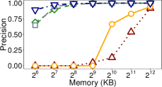
(a) Precision	(b) Recall
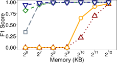
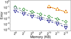
(c) F1 score	(d) Relative error

Figure 2: Experiment 1 (Accuracy for heavy hitter detection).

Experiment 1 (Accuracy for heavy hitter detection). Figure 2 compares the accuracy of MV-Sketch with that of other sketches in heavy hitter detection. Both DEL and FAST have precision and recall near zero when the amount of memory is 512 KB or less, as they need more memory to recover all heavy hitters. Both CMH and LD have high accuracy except when the memory size is only 64 KB, as they incur many false positives in limited memory. Overall, MV-Sketch achieves high accuracy; for example, its relative error is on average 55.8% and 87.2% less than those of LD and CMH, respectively.

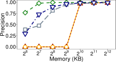
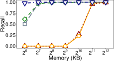
(a) Precision	(b) Recall
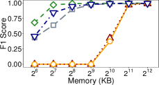
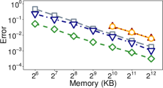
(c) F1 score	(d) Relative error

Figure 3: Experiment 2 (Accuracy for heavy changer detection).

Experiment 2 (Accuracy for heavy changer detection). Figure 3 compares the accuracy of MV-Sketch with that of other sketches in heavy changer detection. Both DEL and FAST again have almost zero precision and recall when the memory size is 512 KB or less. We see that CMH has the highest F1 score and smallest relative error among all sketches, yet its recall is below one for almost all memory sizes. On the other hand, MV-Sketch maintains a recall of one except when the memory size is 64 KB, but its precision is low when the memory size is 256 KB or less. The reason is that MV-Sketch uses the estimated maximum change of a flow for heavy changer detection, thereby having fewer false negatives but more false positives; we view this as a design trade-off. MV-Sketch achieves both higher precision and recall than LD when the memory size is 128 KB or more.

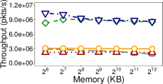
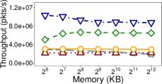
(a) Heavy hitter detection	(b) Heavy changer detection
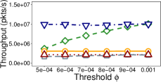
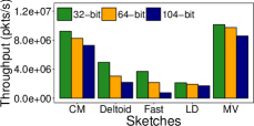
(c) Impact of threshold $\phi$	(d) Impact of key length

Figure 4: Experiment 3 (Update throughput).

Experiment 3 (Update throughput). We now measure the update throughput of all sketches in different settings. We present averaged results over 10 runs. We omit the error bars in our plots as the variances across runs are negligible.

Figure 4(a) shows the update throughput of various sketches in heavy hitter detection. MV-Sketch achieves more than $3\times$ throughput over LD, DEL, and FAST, and 24% higher throughput than CMH when the memory size is 64 KB. Note that MV-Sketch (and other sketches as well) sees a throughput drop as the memory size increases, since it cannot be entirely put in cache and the memory access latency increases. The throughput of CMH is much lower than MV-Sketch, especially when the memory size is 128 KB or less, as it sees many false positives and incurs memory access overhead in its heap.

Figure 4(b) shows the update throughput of various sketches in heavy changer detection. MV-Sketch has the highest throughput, which is 1.34–2.05$\times$ and 2.98–3.38$\times$ over CMH and other sketches, respectively. Note that CMH has lower throughput than in Figure 4(a) although we keep the same number (i.e., 80) of heavy flows in both cases. The reason is that compared to heavy hitter detection, CMH needs to keep more candidates in the heap to guarantee that all heavy changers can be found, thereby incurring higher memory access overhead.

Figure 4(c) shows the impact of the fractional threshold $\phi$ on the update throughput. Here, we focus on heavy hitter detection and fix the memory size as 64 KB. MV-Sketch maintains high and stable throughput (above 9.8 M pkts/s) regardless of the threshold value. CMH has slower throughput for smaller $\phi$ (i.e., more heavy hitters to be detected). For example, when $\phi=$ 0.0005, the throughput of CMH is 3.7M pkts/s only. The reason is that the overhead of maintaining the heap increases with the number of heavy flows being tracked.

Figure 4(d) shows the impact of the key length on the update throughput, by setting the flow keys as source addresses (32 bits), source/destination address pairs (64 bits), and 5-tuples (104 bits). We again focus on heavy hitter detection and fix the memory size as 64 KB. As the key length increases from 32 bits to 104 bits, the throughput drops of MV-Sketch, CMH, and LD are 15-21%, while those of DEL and FAST are 55-80%. The reason is that the numbers of counters in DEL and FAST increase with the key length, thereby incurring much higher memory access overhead.

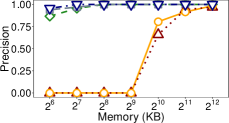
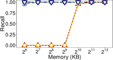
(a) Heavy hitter precision	(b) Heavy hitter recall
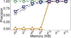
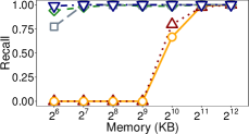
(c) Heavy changer precision	(d) Heavy changer recall

Figure 5: Experiment 4 (Accuracy for scalable detection).

Experiment 4 (Accuracy for scalable detection). Figure 5 shows the precision and recall for scalable heavy flow detection, in which we set $d=3$ and $q=5$. We observe similar results as in Experiments 1 and 2. Note that we also conduct experiments with different combinations of different settings of $d$ and $q$, and the results show similar trends.

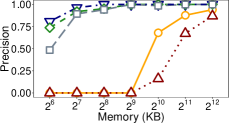
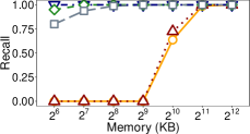
(a) Heavy hitter precision	(b) Heavy hitter recall
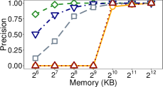
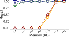
(c) Heavy changer precision	(d) Heavy changer recall

Figure 6: Experiment 5 (Accuracy for network-wide detection).

Experiment 5 (Accuracy for network-wide detection). We compare the accuracy of all sketches in network-wide detection by varying the memory usage in detectors. We randomly partition the 5-minute trace to six detectors, such that the traffic of a flow is distributed in any non-empty subset of the six detectors. Deltoid and Fast Sketch support network-wide detection inherently due to their linear property, in which the counters of different sketch instances with the same index can be added together. For Count-Min-Heap and LD-Sketch, we obtain the estimated sum of each tracked flow key in every detector and aggregate the estimated sums of each flow key. We then use the aggregates for heavy flow detection.

Figure 6 shows the results. Again, we observe similar results as in Experiments 1 and 2. Note that the recall of MV-Sketch is one in all memory sizes for both the heavy hitter and heavy changer detection.

Experiment 6 (Performance optimizations of MV-Sketch). We make a case that MV-Sketch can use SIMD instructions to process multiple data units in parallel and achieve further performance gains. Such performance optimizations enable MV-Sketch to address the need of fast network measurement in software packet processing [34, 32, 25].

Here, we optimize the performance of the update operation (Algorithm 1). Specifically, we divide a hash value into $r$ parts (where $r=4$ in our case). We use SIMD instructions to compute the bucket indices of all $r$ rows, load the $r$ candidate heavy flow keys to a register array, and compare the flow key with the $r$ candidate heavy flow keys in parallel. Based on the comparison results, we update the buckets (Algorithm 1). For 64-bit keys, we use the AVX2 instruction set to manipulate 256 bits (i.e., four 64-bit keys) in parallel.

Figure 7 compares the original and optimized implementations of MV-Sketch. The optimized version achieves 75% higher throughput than the original version on average. Its throughput is above 14.88M pkts/s in most cases, implying that it can match the 10 Gb/s line rate (Section I).

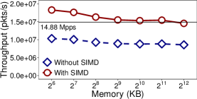
Figure 7: Experiment 6 (Performance optimizations of MV-Sketch).

VI-B Evaluation in Hardware

We prototype MV-Sketch in P4 [10] and compile it to the Barefoot Tofino chipset [45].

Testbed. Our testbed consists of two servers and a Barefoot Tofino switch. Each server has two 12-core 2.2 GHz CPUs, 32 GB RAM, and a 40 Gbps NIC, while the switch has 32 100 Gb ports. The two servers are connected via the switch, where the traffic from one server is directly forwarded to the other via the switch.

Methodology. We compare MV-Sketch with PRECISION [7], which is designed for heavy hitter detection in programmable switches. PRECISION tracks heavy hitters by probabilistically recirculating a small fraction of packets. We compare MV-Sketch and PRECISION for both packet counting and size counting. We use the same CAIDA trace as in Section VI-A.

We fix MV-Sketch as $r=1$ row and 2,048 buckets. Our software evaluation (Section VI-A) shows that with such a configuration, MV-Sketch achieves an accuracy of above 0.9 for various epoch lengths. We configure PRECISION with 2-way associativity to balance between the accuracy and the number of pipelined stages, and fix its memory usage to be the same as that of MV-Sketch. By default, we use source IPv4 addresses as flow keys.

We use the built-in hash function CRC32 [19] in our switch as the hash function in sketches. We find that both MurmurHash [3] (used in our software evaluation) and CRC32 have nearly identical accuracy results in our evaluation, yet MurmurHash has much higher update throughput than CRC32. Thus, we use MurmurHash in software evaluation, while using CRC32 here in hardware evaluation.

Experiment 7 (Switch resource usage). We measure the switch resource usage of MV-Sketch and PRECISION. We prototype PRECISION and each version of MV-Sketch (i.e., Algorithm 4 for 5-tuple flow keys (MVFULL) and Algorithm 5 for size counting on 32-bit flow keys (MVSC), and Algorithm 6 for packet counting on 32-bit flow keys (MVPC)). Note that PRECISION considers only 32-bit flow keys.

TABLE II: Experiment 7: Switch resource usage (percentages in brackets are fractions of total resource usage).

	MVFULL	MVSC	MVPC	PRECISION
SRAM (KiB)	144 (0.94%)	80 (0.52%)	80 (0.52%)	192 (1.25%)
No. stages	4 (33.33%)	2 (16.67%)	1 (1.33%)	8 (66.67%)
No. actions	10	5	3	15
No. ALUs	3 (6.25%)	2 (4.17%)	2 (4.17%)	6 (12.5%)
PHV (bytes)	133 (17.32%)	108 (14.06%)	102 (13.28%)	137 (17.84%)

Table II shows the switch resource usage in terms of SRAM usage (which measures memory usage), the numbers of physical stages, actions, and stateful ALUs (all of which measure computational resources), as well as the PHV size (which measures the message size across stages). All the MV-Sketch implementations achieve less resource usage than PRECISION.

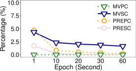
Figure 8: Experiment 8 (Switch throughput analysis). Here, we show the percentage of packets being recirculated to the second pass of the switch pipeline.

Experiment 8 (Switch throughput analysis). We study the throughput of MV-Sketch and PRECISION. We split the trace into one-second epochs and randomly select 50 epochs. We replay each epoch in one server with Pktgen-DPDK [38] and compute the average receiving rate in another server with the DPDK programs. We consider two implementation approaches of recirculating packets within the switch pipeline: (i) using the recirculate primitive to recirculate packets via the dedicated recirculation ports of the switch, and (ii) using the resubmit primitive to recirculate packets within the ingress pipeline via normal ports. For the first approach, both MV-Sketch and PRECISION achieve the line rate in all cases. For the second approach, MV-Sketch achieves the line rate for packet counting and 95% of the line rate in size counting, while PRECISION achieves around 98% of the line rate for both packet counting and size counting (not shown in figures).

To further examine the recirculation costs of MV-Sketch and PRECISION in size counting (denoted by MVSC and PRESC, respectively) and packet counting (denoted by MVPC and PREPC, respectively), we conduct software simulation that measures the percentage of packets that are recirculated to the second pass of the switch pipeline in an epoch for each approach. Figure 8 shows the results for different epoch lengths; since the variance of the percentage for each approach is small, we omit the error bars here. MV-Sketch has zero percentage for packet counting by design. Also, it has a higher percentage than PRECISION in size counting, yet the percentage is below 5% in all cases and shows a downward trend as the epoch length increases. The percentage of PRECISION in both packet counting and size counting is below 2% in almost all cases.

Experiment 9 (Accuracy comparisons between MV-Sketch and PRECISION). We study the accuracy of MV-Sketch and PRECISION for heavy hitter detection in software simulation by varying the epoch lengths. Figure 9 shows the results. MV-Sketch achieves higher accuracy than PRECISION in size counting for all epochs (in F1-score and relative errors), and has a comparable F1-score with PRECISION in packet counting. The relative error of MV-Sketch is higher than PRECISION in packet counting, yet the difference is small as the highest error of MV-Sketch is less than 1.6% in our evaluation. PRECISION performs much better in packet counting than in size counting. The reason is that the counter value of each flow in size counting is much larger than that in packet counting, and hence leads to a smaller recirculating probability and causes PRECISION to miss more packets in size counting.

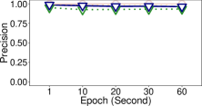
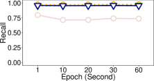
(a) Precision	(b) Recall
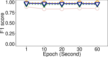
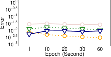
(c) F1 score	(d) Relative error

Figure 9: Experiment 9 (Accuracy comparisons between MV-Sketch and PRECISION).

VII Related Work

Invertible sketches. In Section II-B, we review several invertible sketches for heavy flow detection and their limitations. Another related work extends the Bloom filter [9] with invertibility [20, 22]. In particular, the Invertible Bloom Lookup Table (IBLT) [22] tracks three variables in each bucket: the number of keys, the sum of keys, and the sum of values for all keys hashed to the bucket. To recover all hashed keys, it iteratively recovers from the buckets with only one hashed key and deletes the hashed key of all its associated buckets (so that some buckets now have one hashed key remaining). FlowRadar [32] builds on IBLT for heavy flow detection. However, IBLT is sensitive to hash collisions: if multiple keys are hashed to the same bucket, it fails to recover the keys in the bucket.

A closely related work to ours is AMON [29], which applies MJRTY in heavy hitter detection. However, AMON and MV-Sketch have different designs: AMON splits a packet stream into multiple sub-streams and tracks the candidate heavy flow for each sub-stream using MJRTY, while MV-Sketch maps each packet to the buckets in different rows in a sketch data structure. MV-Sketch addresses the following issues that are not considered by AMON: (i) providing theoretical guarantees on the trade-offs across memory usage, update/detection performance, and detection accuracy; and (ii) addressing heavy changer detection and network-wide detection.

Sketch-based network-wide measurement. Recent studies [48, 36, 34, 32, 25, 46, 27] propose sketch-based network-wide measurement systems for general measurement tasks, including heavy flow detection. Such systems leverage a centralized control plane to analyze measurement results from multiple sketches in the data plane. Our work focuses on a compact invertible sketch design that targets both heavy hitter and heavy changer detection.

Counter-based algorithms. Some approaches [35, 30, 43, 5, 6, 47] track the most frequent flows in counter-based data structures (e.g., heaps and associative arrays), which dynamically admit or evict flows based on estimated flow sizes. They target heavy hitter detection, but do not consider heavy changer detection and network-wide detection.

Measurement in programmable switches. Recent work focuses on pushing measurement algorithms from end hosts to programmable switches [42, 28, 39, 43, 24, 7], subject to the switch hardware constraints. Our work demonstrates that MV-Sketch can be feasibly deployed in programmable switches to detect heavy flows with limited resource overhead.

VIII Conclusion

MV-Sketch is an invertible sketch designed for fast and accurate heavy flow detection. It builds on the majority vote algorithm to enhance memory management in two aspects: (i) small and static memory allocation, and (ii) lightweight memory access in both update and detection operations. It can also be generalized for both scalable and network-wide detection. Trace-driven evaluation in software demonstrates the throughput and accuracy gains of MV-Sketch. We also show how the update performance of MV-Sketch can be boosted via SIMD instructions. Evaluation in hardware demonstrates that MV-Sketch can be feasibly implemented in programmable switches with limited resource overhead.

References

- [1] O. Alipourfard, M. Moshref, Y. Zhou, T. Yang, and M. Yu. A Comparison of Performance and Accuracy of Measurement Algorithms in Software. In Proc. of ACM SOSR, 2018.
- [2] M. Alizadeh, T. Edsall, S. Dharmapurikar, R. Vaidyanathan, K. Chu, A. Fingerhut, F. Matus, R. Pan, N. Yadav, G. Varghese, et al. CONGA: Distributed Congestion-Aware Load Balancing for Datacenters. In Proc. of ACM SIGCOMM, 2014.
- [3] A. Appleby. https://github.com/aappleby/smhasher.
- [4] R. B. Basat, G. Einziger, R. Friedman, and Y. Kassner. Heavy Hitters in Streams and Sliding Windows. In Proc. of IEEE INFOCOM, 2016.
- [5] R. B. Basat, G. Einziger, R. Friedman, and Y. Kassner. Optimal Elephant Flow Detection. In Proc. of IEEE INFOCOM, 2017.
- [6] R. B. Basat, G. Einziger, R. Friedman, and Y. Kassner. Randomized Admission Policy for Efficient Top-k and Frequency Estimation. In Proc. of IEEE INFOCOM, 2017.
- [7] R. Ben-Basat, X. Chen, G. Einziger, and O. Rottenstreich. Efficient Measurement on Programmable Switches Using Probabilistic Recirculation. In Proc. of IEEE ICNP, 2018.
- [8] T. Benson, A. Anand, A. Akella, and M. Zhang. MicroTE: Fine Grained Traffic Engineering for Data Centers. In Proc. of ACM CoNEXT, 2011.
- [9] B. H. Bloom. Space/time Trade-offs in Hash Coding with Allowable Errors. Communications of the ACM, 13(7):422–426, 1970.
- [10] P. Bosshart, D. Daly, G. Gibb, M. Izzard, N. McKeown, J. Rexford, C. Schlesinger, D. Talayco, A. Vahdat, G. Varghese, et al. P4: Programming protocol-independent packet processors. ACM SIGCOMM Computer Communication Review, 44(3):87–95, 2014.
- [11] P. Bosshart, G. Gibb, H.-S. Kim, G. Varghese, N. McKeown, M. Izzard, F. Mujica, and M. Horowitz. Forwarding Metamorphosis: Fast Programmable Match-Action Processing in Hardware for SDN. ACM SIGCOMM Computer Communication Review, 43(4):99–110, 2013.
- [12] R. S. Boyer and J. S. Moore. MJRTY - A Fast Majority Vote Algorithm. In Automated Reasoning, pages 105–117. Springer, 1991.
- [13] T. Bu, J. Cao, A. Chen, and P. P. C. Lee. Sequential Hashing: A Flexible Approach for Unveiling Significant Patterns in High Speed Networks. Computer Networks, 54(18):3309–3326, 2010.
- [14] CAIDA. http://www.caida.org.
- [15] M. Charikar, K. Chen, and M. Farach-Colton. Finding Frequent Items in Data Streams. In Proc. of ICALP, 2002.
- [16] G. Cormode and S. Muthukrishnan. An Improved Data Stream Summary: The Count-min Sketch and its Applications. Journal of Algorithms, 55(1):58–75, 2005.
- [17] G. Cormode and S. Muthukrishnan. Space Efficient Mining of Multigraph Streams. In Proc. of ACM PODS, 2005.
- [18] G. Cormode and S. Muthukrishnan. What’s New: Finding Significant Differences in Network Data Streams. IEEE/ACM Trans. on Networking, 13(6):1219–1232, 2005.
- [19] CRC32. https://github.com/d-bahr/CRCpp.
- [20] D. Eppstein and M. T. Goodrich. Straggler Identification in Round-Trip Data Streams via Newton’s Identities and Invertible Bloom Filters. IEEE Trans. on Knowledge and Data Engineering, 23(2):297–306, 2011.
- [21] P. Garcia-Teodoro, J. Diaz-Verdejo, G. Maciá-Fernández, and E. Vázquez. Anomaly-Based Network Intrusion Detection: Techniques, Systems and Challenges. Computers & Security, 28(1-2):18–28, 2009.
- [22] M. T. Goodrich and M. Mitzenmacher. Invertible Bloom Lookup Tables. arXiv, 2015. https://arxiv.org/abs/1101.2245.
- [23] A. Gupta, R. Harrison, M. Canini, N. Feamster, J. Rexford, and W. Willinger. Sonata: Query-Driven Streaming Network Telemetry. In Proc. of ACM SIGCOMM, 2018.
- [24] R. Harrison, Q. Cai, A. Gupta, and J. Rexford. Network-Wide Heavy Hitter Detection with Commodity Switches. In Proc. of ACM SOSR, 2018.
- [25] Q. Huang, X. Jin, P. P. C. Lee, R. Li, L. Tang, Y.-C. Chen, and G. Zhang. SketchVisor: Robust Network Measurement for Software Packet Processing. In Proc. of ACM SIGCOMM, 2017.
- [26] Q. Huang and P. P. C. Lee. A Hybrid Local and Distributed Sketching Design for Accurate and Scalable Heavy Key Detection in Network Data Streams. Computer Networks, 91(11):298–315, 2015.
- [27] Q. Huang, P. P. C. Lee, and Y. Bao. SketchLearn: Relieving User Burdens in Approximate Measurement with Automated Statistical Inference. In Proc. of ACM SIGCOMM, 2018.
- [28] X. Jin, X. Li, H. Zhang, R. Soulé, J. Lee, N. Foster, C. Kim, and I. Stoica. NetCache: Balancing Key-Value Stores with Fast In-Network Caching. In Proc. of SOSP, 2017.
- [29] M. Kallitsis, S. A. Stoev, S. Bhattacharya, and G. Michailidis. AMON: An Open Source Architecture for Online Monitoring, Statistical Analysis, and Forensics of Multi-Gigabit Streams. IEEE Journal on Selected Areas in Communications, 34(6):1834–1848, 2016.
- [30] R. M. Karp, S. Shenker, and C. H. Papadimitriou. A Simple Algorithm for Finding Frequent Elements in Streams and Bags. ACM Trans. on Database Systems, 28(1):51–55, 2003.
- [31] B. Krishnamurthy, S. Sen, Y. Zhang, and Y. Chen. Sketch-based Change Detection: Methods, Evaluation, and Applications. In Proc. of ACM IMC, 2003.
- [32] Y. Li, R. Miao, C. Kim, and M. Yu. FlowRadar: a Better NetFlow for Data Centers. In Proc. of USENIX NSDI, 2016.
- [33] Y. Liu, W. Chen, and Y. Guan. A Fast Sketch for Aggregate Queries over High-Speed Network Traffic. In Proc. of IEEE INFOCOM, 2012.
- [34] Z. Liu, A. Manousis, G. Vorsanger, V. Sekar, and V. Braverman. One Sketch to Rule Them All: Rethinking Network Flow Monitoring with UnivMon. In Proc. of ACM SIGCOMM, 2016.
- [35] J. Misra and D. Gries. Finding Repeated Elements. Science of computer programming, 2(2):143–152, 1982.
- [36] M. Moshref, M. Yu, R. Govindan, and A. Vahdat. SCREAM: Sketch Resource Allocation for Software-defined Measurement. In Proc. of ACM CoNEXT, 2015.
- [37] J. Nelson and D. P. Woodruff. Fast Manhattan Sketches in Data Streams. In Proc. of ACM PODS, 2010.
- [38] Pktgen-DPDK. http://pktgen-dpdk.readthedocs.io/en/latest/.
- [39] A. Sapio, I. Abdelaziz, A. Aldilaijan, M. Canini, and P. Kalnis. In-Network Computation is A Dumb Idea Whose Time Has Come. In Proc. of ACM HotNets, 2017.
- [40] R. Schweller, Z. Li, Y. Chen, Y. Gao, A. Gupta, Y. Zhang, P. Dinda, M. Y. Kao, and G. Memik. Reversible Sketches: Enabling Monitoring and Analysis over High-Speed Data Streams. IEEE/ACM Trans. on Networking, 15(5):1059–1072, 2007.
- [41] A. Sivaraman, A. Cheung, M. Budiu, C. Kim, M. Alizadeh, H. Balakrishnan, G. Varghese, N. McKeown, and S. Licking. Packet Transactions: High-Level Programming for Line-Rate Switches. In Proc. of ACM SIGCOMM, 2016.
- [42] A. Sivaraman, C. Kim, R. Krishnamoorthy, A. Dixit, and M. Budiu. DC. p4: Programming the Forwarding Plane of A Data-Center Switch. In Proc. of ACM SOSR, 2015.
- [43] V. Sivaraman, S. Narayana, O. Rottenstreich, S. Muthukrishnan, and J. Rexford. Heavy-Hitter Detection Entirely in the Data Plane. In Proc. of ACM SOSR, 2017.
- [44] L. Tang, Q. Huang, and P. P. Lee. MV-Sketch: A Fast and Compact Invertible Sketch for Heavy Flow Detection in Network Data Streams. In Proc. of IEEE INFOCOM, 2019.
- [45] Tofino. https://barefootnetworks.com/products/brief-tofino/.
- [46] T. Yang, J. Jiang, P. Liu, Q. Huang, J. Gong, Y. Zhou, R. Miao, X. Li, and S. Uhlig. Elastic Sketch: Adaptive and Fast Network-Wide Measurements. In Proc. of ACM SIGCOMM, 2018.
- [47] T. Yang, H. Zhang, J. Li, J. Gong, S. Uhlig, S. Chen, and X. Li. HeavyKeeper: An Accurate Algorithm for Finding Top-k Elephant Flows. IEEE/ACM Trans. on Networking, 27(5):1845–1858, 2019.
- [48] M. Yu, L. Jose, and R. Miao. Software Defined Traffic Measurement with OpenSketch. In Proc. of USENIX NSDI, 2013.
- [49] Y. Zhang, L. Breslau, V. Paxson, and S. Shenker. On the Characteristics and Origins of Internet Flow Rates. In Proc. of ACM SIGCOMM, 2002.
- [50] Q. Zhao, A. Kumar, and J. Xu. Joint Data Streaming and Sampling Techniques for Detection of Super Sources. In Proc. of ACM IMC, 2005.