A Surrogate Model for Gravitational Wave Signals from Comparable- to Large- Mass-Ratio Black Hole Binaries

Abstract

Gravitational wave signals from compact astrophysical sources such as those observed by LIGO and Virgo require a high-accuracy, theory-based waveform model for the analysis of the recorded signal. Current inspiral-merger-ringdown models are calibrated only up to moderate mass ratios, thereby limiting their applicability to signals from high-mass ratio binary systems. We present EMRISur1dq1e4, a reduced-order surrogate model for gravitational waveforms of $13,500M$ in duration and including several harmonic modes for non-spinning black hole binary systems with mass-ratios varying from $3$ to $10,000$ thus vastly expanding the parameter range beyond the current models. This surrogate model is trained on waveform data generated by point-particle black hole perturbation theory (ppBHPT) both for large mass-ratio and comparable mass-ratio binaries. We observe that the gravitational waveforms generated through a simple application of ppBHPT to the comparable mass-ratio cases agree surprisingly well with those from full numerical relativity after a rescaling of the ppBHPT’s total mass parameter. This observation and the EMRISur1dq1e4 surrogate model will enable data analysis studies in the high-mass ratio regime, including potential intermediate mass-ratio signals from LIGO/Virgo and extreme-mass ratio events of interest to the future space-based observatory LISA.

Introduction – As the LIGO Aasi et al. (2015) and Virgo Acernese et al. (2015) detectors improve their sensitivity, gravitational wave (GW) detections Abbott et al. (2016a, 2017a, b, 2017b, 2017c, 2017d, 2018a) are becoming routine Abbott et al. (2018b, c). In the current observing run, for example, gravitational-wave events are now being detected multiple times a month ale . Among the most important sources for these detectors are binary black hole (BBH) systems, in which two black holes (BHs) radiate energy through GWs, causing them to inspiral, merge, and finally settle down into a single black hole through a ringdown phase.

To date all LIGO/Virgo events show support only for systems with mass ratios $q=m_{1}/m_{2}<8$ Abbott et al. (2019). Nevertheless, one should expect to observe larger mass ratio systems in the future. For example, the first and second observing runs Abbott et al. (2019) have already observed compact objects over a mass range of $1.3M_{\odot}$ to $85M_{\odot}$ suggesting combinations involving mass-ratios in the range of $10$ to $20$ are not unreasonable for LIGO/Virgo to detect, especially, if the lighter member of the binary is a neutron star or for BBH systems within the accretion disks of Active Galactic Nuclei McKernan et al. (2019). A third generation (3G) ground-based detector, like the Einstein Telescope or Cosmic Explorer Hild et al. (2011); Kalogera et al. (2019); Vitale and Evans (2017), may be able to reach up to redshifts beyond 10 and with an improved low-frequency sensitivity limit, implying an increased rate of detection of BBH events with unequal mass ratios Amaro-Seoane (2018); Reitze et al. (2019). Intermediate mass ratio inspirals are also one of the key target sources of the future LISA space-based gravitational wave Miller (2009); Hughes (2006); Amaro-Seoane et al. (2007) detector along with extreme mass ratio systems comprised of a small compact body (possibly a neutron star or stellar mass black hole) orbiting a supermassive black hole (at a galactic center) Hughes (2006); Amaro-Seoane et al. (2017); Gair et al. (2004); Amaro-Seoane et al. (2007).

In all of these cases we need accurate and fast-to-evaluate inspiral-merger-ringdown (IMR) models covering a range of large- to extreme- mass ratio systems. Such models are needed to maximize the science output of data collected by ground-based detectors or to perform mock data analysis studies for LISA and 3G detectors.

Successful detection and parameter estimation relies on being able to compute, from accurate numerical relativity (NR) simulations, the detailed waveform signal template for such systems. Because solving the Einstein field equations for thousands to millions of potential astrophysical sources is exceedingly challenging, several approximate waveform models that are much faster to evaluate have been developed Khan et al. (2018); Cotesta et al. (2018); London et al. (2018); Pan et al. (2014); Bohe et al. (2017); Khan et al. (2016); Hannam et al. (2014); Taracchini et al. (2014a); Pan et al. (2011); Mehta et al. (2017); Babak et al. (2017); Damour et al. (2013); Bernuzzi and Nagar (2010); Bernuzzi et al. (2011a, b); Nagar et al. (2018), including an effective one body model Taracchini et al. (2013, 2014b) calibrated up to $q=100$ using results from black hole perturbation theory  Bohe et al. (2017). These models assume an underlying phenomenology based on physical considerations, and calibrate any remaining free parameters to NR simulations. Within the LISA waveform modelling community, the computational expense of perturbation-theory waveforms presents a similar bottleneck. By relying on a combination of approximations, progress has been make towards the development of “kludge” models which can generate waveforms quickly while capturing the qualitative features of extreme mass ratio inspiral (EMRI) waveforms Barack and Cutler (2004); Babak et al. (2007); Barack and Cutler (2004); Chua et al. (2017); Chua and Gair (2015).

Surrogate modeling Field et al. (2014); Purrer (2014) is an alternative approach that doesn’t assume an underlying phenomenology and has been applied to a diverse range of problems Field et al. (2014); Purrer (2014); Lackey et al. (2017); Doctor et al. (2017); Blackman et al. (2015, 2017a, 2017b); Huerta et al. (2018); Chua et al. (2018); Canizares et al. (2015); Galley and Schmidt (2016); Varma et al. (2019a, b, c); Chua et al. (2018); Lackey et al. (2019a); Bohe et al. (2017); Lackey et al. (2019b). These models follow a data-driven learning strategy, directly using waveform training data collected by running numerically expensive partial differential equation (PDE) solvers. Surrogate models are accurate in the region of parameter space over which they were trained as well as extremely fast to evaluate. For example, for our model the underlying solver used to generate a single training waveform takes about 2 hours while its corresponding surrogate can be evaluated in under a second.

Modeling IMR signal templates for black hole binary systems with moderate to large mass ratios has remained challenging. One practical reason is that comparable-mass binaries, a dominant source for currently operational ground-based detectors, have received significant attention from the waveform modeling community. Furthermore, this is a parameter regime that is particularly challenging for NR as the small length scales introduced by the smaller BH impose a very high grid resolution requirement. In the extreme cases, i.e. when one black hole is supermassive like those at the center of most galaxies, the mass-ratio may approach $q\sim 10^{9}$. These are well beyond the scope of NR and are typically well-suited for black hole perturbation theory.

In this Letter we present a surrogate model for gravitational waveforms emitted from non-spinning black hole binary systems that span an extremely wide range of mass-ratios, from $q=3$ to $q=10,000$. This is the first surrogate model that covers such a wide range of mass-ratios. The model includes all of the phases of the system’s evolution starting from a slow inspiral through plunge and ringdown, and includes not only the dominant quadrupole mode, but also several of the most important higher harmonic modes that are especially important at larger mass ratio Varma and Ajith (2017); Bustillo et al. (2018); Pang et al. (2018); Littenberg et al. (2013); Kalaghatgi et al. (2019). The model spans $13,500M$ in duration, which for a $q=10$ and $q=10^{4}$ system corresponds to $32$ and $144$ orbital cycles, respectively. This model can be immediately used in data analysis studies or phenomenological model building efforts that involve large-mass ratio systems, and serves as a proof-of-principle that the surrogate modeling methodology developed for LIGO-type sources remain applicable for LISA-type sources. In future work we will extend our model to include spinning BHs and more orbits.

The training data we use to build this reduced-order surrogate model is generated using the point-particle black hole perturbation theory (ppBHPT) framework, i.e. a high-performance Teukolsky equation Teukolsky (1973) solver code (using a point-particle source) in the time-domain Sundararajan et al. (2007, 2008, 2010); Zenginoğlu and Khanna (2011). While black hole perturbation theory’s domain of validity is typically taken to be very high mass-ratio binaries, it is interesting to note that a simple rescaling of the mass parameter is sufficient to achieve accurate agreement with NR waveforms for mass-ratios less than $10$. That perturbation-theory waveforms agree at all with NR for small-mass ratio systems is somewhat remarkable given that this regime is typically considered beyond perturbation theory’s domain of validity.

Background on ppBHPT – In the context of the large mass-ratio limit of a black hole binary system, the system’s dynamics can be described using Kerr black hole perturbation theory. In this approach, the smaller black hole is modeled as a point-particle with no internal structure, moving in the space-time of the larger Kerr black hole. Gravitational radiation is computed by evolving the perturbations generated by solving the Teukolsky master equation with a particle-source Sundararajan et al. (2007, 2008, 2010); Zenginoğlu and Khanna (2011).

We implemented this ppBHPT approach in two steps. First, we compute the trajectory taken by the point-particle, and then we use that trajectory to compute the gravitational wave emission. For the first step, the particle’s motion can be characterized by three distinct regimes – an initial adiabatic inspiral, in which the particle follows a sequence of geodesic orbits, driven by radiative energy and angular momentum losses computed by solving the frequency-domain Teukolsky equation Fujita and Tagoshi (2004, 2005); Mano et al. (1996); Throwe (2010) with an open-source code GremlinEq gre ; O’Sullivan and Hughes (2014); Drasco and Hughes (2006); a late-stage geodesic plunge into the horizon; and a transition regime between those two Ori and Thorne (2000); Hughes et al. (2019); Sundararajan et al. (2010); Apte and Hughes (2019) For the low mass-ratio cases, unsurprisingly, the Ori-Thorne transition trajectory algorithm doesn’t perform very well. This results in a small jump in the velocities of the point-particle as it exits the adiabatic inspiral and also when it begins the plunge. This jump results in some small unphysical oscillations in the waveforms, especially in some of the higher-order modes. We correct for this by using a “smoothening” procedure. It should be noted that our trajectory model does not include the effects of the conservative or second-order self-force Hinderer and Flanagan (2008), although once these post-adiabatic corrections are known (see, for example, Refs. Gralla (2012); Pound (2012); Pound et al. (2019)) they could be easily incorporated to improve the accuracy of the inspiral’s phase.

With the trajectory of the perturbing compact body fully specified, we then solve the inhomogeneous Teukolsky equation in the time-domain while feeding the trajectory information from the first step into the particle source-term of the equation. In particular, (i) we first rewrite the Teukolsky equation using compactified hyperboloidal coordinates that allow us to extract the gravitational waveform directly at null infinity while also solving the issue of unphysical reflections from the artificial boundary of the finite computational domain; (ii) we take advantage of axisymmetry of the background Kerr space-time, and separate the dependence on azimuthal coordinate, thus obtaining a set of (2+1) dimensional PDEs; (iii) we then recast these equations into a first-order, hyperbolic PDE system; and in the last step (iv) we implement a two-step, second-order Lax-Wendroff, time-explicit, finite-difference numerical evolution scheme. The particle-source term on the right-hand-side of the Teukolsky equation requires some specialized techniques for such a finite-difference numerical implementation and, for technical reasons, we set the spin of the central black hole ($a=10^{-6}$) sufficiently close to zero. Additional details can be found in our earlier work Sundararajan et al. (2007, 2008, 2010); Zenginoğlu and Khanna (2011) and the associated references. Our numerical evolution scheme is implemented using OpenCL/CUDA-based GPGPU-computing which allows for very long duration and high-accuracy computations within a reasonable time-frame. Numerical errors in the phase and amplitude are typically on the scale of a small fraction of a percent McKennon et al. (2012) (cf. Fig. 1).

Description of the Surrogate Model EMRISur1dq1e4– Our surrogate model is built using a combination of methodologies proposed in previous works Blackman et al. (2015); Field et al. (2014); Purrer (2014), which we briefly summarize here.

We collect our waveform training data by numerically solving the inhomogeneous Teukolsky equation at 37 different values of the mass ratio $q$ (cf. the bottom panel of Fig. 1) and for each value of $q$ extract the harmonic modes, $h^{\ell,m}(t;q)$, for $(\ell,m)=\{(2,\{2,1\}),(3,\{3,2,1\}),(4,\{4,3,2\}),(5,\{5,4,3\})\}$. Following Blackman et al. (2015), we enact a time shift and physical rotation about the z-axis such that (i) each waveform’s time is shifted such that $t=0$ occurs at the peak of the the (2,2) mode’s amplitude, $\left|h^{22}\right|$, and (ii) all the modes’ phases are aligned by performing a frame rotation about the z-axis such that at the start of the waveform $\phi^{22}=0$ and $\phi^{21}\in(-\pi,0]$, where $\phi^{22}$ and $\phi^{21}$ are the phases of the complex $h^{2,2}$ and $h^{2,1}$ modes, respectively. This pre-processing alignment step ensures that all of the training-set waveforms now depend smoothly on the parameter $q$.

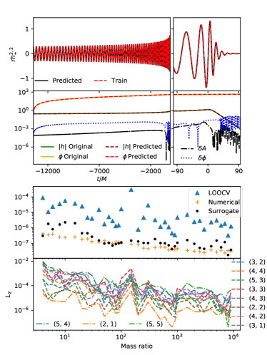
Figure 1: The bottom subfigure depicts each mode’s relative error by comparing the surrogate model and the training data. The relative error is computed from Eq. (3) with $\alpha=1$ and using the appropriate mode in place of where it says “$h^{22}"$. The penultimate subfigure shows the numerical truncation errors (orange plus) estimate the quality of the training waveform data by comparing two numerical simulations of increasing resolution. We also compared the full surrogate (including all $11$ harmonic modes) and the training data (black circles) and a leave-one-out cross-validation (LOOCV) trial surrogate and the training data (blue triangles). The largest LOOCV error is for q = 4, for which the $h_{+}$ polarization’s quadrupole mode is shown in the top subfigure. The second subfigure reports on the error in the amplitude and phase for this case; our full surrogate, trained on the entire data set of $37$ waveforms, is more accurate than the LOOCV diagnostics shown.

After alignment we decompose the waveform into data pieces which are simpler to model. In our case, we choose the waveform modes’ amplitude and phase as our data pieces, and interpolate these onto a time grid $\left[-13404,94\right]$M with $\Delta t=0.05$M. Following Refs. Blackman et al. (2015); Field et al. (2014), we construct an empirical interpolant (EI) Maday et al. (2009); Chaturantabut and Sorensen (2010) (an interpolant whose basis and nodes are learned by applying optimization methods to the training set) for each data piece; there are 11 modes provided by the ppBHPT solver and so we construct $22$ empirical interpolants in total (cf. Eq. 3 of Ref. Blackman et al. (2015)). Note that we model $m>0$ modes only since the negative modes, $h^{\ell,-m}=(-1)^{\ell}h^{\ell,m}{}^{*}$, are related to the positive modes due to symmetry of the system under reflections about the orbital plane.

The empirical interpolant gives a compact representation for each data piece (and hence the full waveform) in the training set by permitting the full time-series to be reconstructed through a significantly sparser sampling defined by the EI nodes. To predict new waveforms not in the training set, at each EI node we model the data pieces’ parametric dependence on $q$ with a spline Purrer (2014).

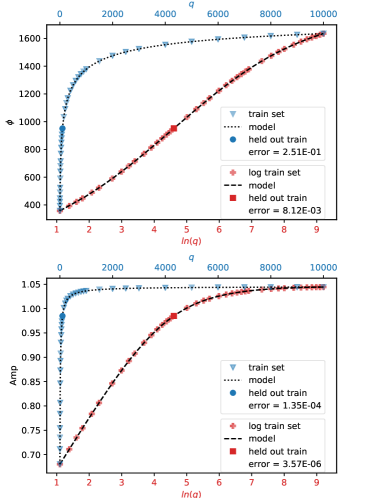
Figure 2: At each empirical interpolation node we build surrogate models for amplitude, $A^{2,2}(q)\approx A_{\tt S}^{2,2}(q)$, and phase $\phi^{2,2}(q)\approx\phi_{\tt S}^{2,2}(q)$ across the training region. One of the key methodological improvements pursued here is modeling the training data after performing a logarithmic transformation (red asterisk) of the independent variable $\{\ln(q),A^{2,2}(q)\}$ and $\{\ln(q),\phi^{2,2}(q)\}$. Here we show the LOOCV model error at $q=100$, which leads to nearly two orders of magnitude improvement as compared with no transformation (blue triangle). Data for the other harmonic modes and empirical interpolation node data show similar improvement.

Two examples are given in Fig 2, where we show the training data and model for the $(2,2)$ mode’s amplitude and phase at some randomly selected EI node; by fixing the time this data is a function of $q$ only. Our data-piece models are built using degree 2 interpolating splines without any smoothing factors. As shown in Fig. 2 we find significantly better accuracy when modeling the data after performing a logarithmic transformation of the independent variable. This was first used in Refs. Varma et al. (2019b, c), and we suspect this will be important for any model seeking to cover large ranges of the mass ratio. The remaining $10$ subdominant modes follow the same approach.

When evaluating the surrogate waveform, we first evaluate each surrogate waveform data piece at the requested value of $q$ and use the EI representation to reconstruct the surrogate prediction for the waveform as a dense time-series. The full surrogate, $h_{\tt S}$, can be written as

$$h_{\tt S}(t,\theta,\phi;q)=\sum_{\ell,m}h_{\tt S}^{\ell,m}(t;q){}_{-2}Y_{\ell m}(\theta,\phi)\,,$$ (1)

where ${}_{-2}Y_{\ell m}$ are the spin ($-2$) weighted spherical harmonics and models for each harmonic mode (a single complex function), $h_{\tt S}^{\ell,m}(t;q)=A_{\tt S}^{\ell,m}(t;q)\exp(-\mathrm{i}\phi_{\tt S}^{\ell,m}(t;q))$, are defined in terms of models of the amplitude and phases (two real functions).

To assess the surrogate model’s error, we perform some of the tests described in Ref. Blackman et al. (2017c) using a relative $L_{2}$-type norm (we compute the norm of the error through a time-domain overlap integral with a white-noise curve) given exactly by Eq. (21) in Ref.  Blackman et al. (2017c). This measures the full waveform Eq. (1) error over the sphere and automatically includes error contributions from all of the harmonic modes. In Fig. 1 we (i) check that the surrogate model can reproduce all 37 ppBHPT waveforms used to train the surrogate (black circles), (ii) perform a leave-one-out cross validation study to asses the model’s ability to predict new waveforms it was not trained on (blue triangles), and (iii) compare both errors to the numerical truncation error of the Teukolsky solver used to produce the training data (orange plus). We find that the model errors remain extremely small over the range of mass ratios $q=3$ to $10^{4}$, although a they are a bit larger than the errors in the training data itself. We remind the reader that these comparisons are between the model, EMRISur1dq1e4, and the output of the Teukolsky solver. Waveforms generated within the ppBHPT framework are expected to become more accurate as $q$ becomes large. Next we provide evidence for using ppBHPT waveforms even at small mass ratios.

Waveforms from Comparable Mass Binaries using Perturbation Theory – We now proceed to compare the model output with full NR data. This comparison is naturally restricted to low mass-ratios $q\leq 10$. For the high mass-ratio cases, extensive comparisons with EOB have been performed previously in the context of the EMRI data itself Barausse et al. (2012), so we do not focus on those cases. Additionally, there is a lack of models and data for the intermediate ranges, say from $q=10$ to $q=10^{4}$, so we leave that domain open for future comparisons.

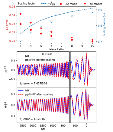
Figure 3: Waveform difference between numerical relativity and ppBHPT waveforms before and after rescaling the ppBHPT’s total mass parameter. Bottom panel: These two figures focus on the case $q=8$. Before rescaling the NR (solid blue) and ppBHPT (dashed red) waveforms are noticeably different in both their amplitude and phasing and have an L2 difference of $7.03\times 10^{-1}$. We find the optimum value of the rescaling parameter to be $\alpha=0.85837$ and modify the ppBHPT waveform according to Eq. (2). After rescaling the NR and modified ppBHPT waveforms demonstrate remarkable agreement with one another. Top panel: We repeat this comparison procedure for mass ratios $3\leq q\leq 10$ where NR data is available, and compute both the optimal scaling factor and the L2 difference between waveforms (NR vs scaled ppBHPT) for each case. In all cases the differences before rescaling are order unity, while the agreement between the rescaled ppBHPT and NR waveforms is $\approx 1$%. The dotted line refers to a naive value of $\alpha=1/(1+1/q)$ set by including the mass the of smaller black hole as part of the background spacetime.

One complication that appears when we attempt to perform a careful comparison with NR is how to set an overall mass-scale for the comparison and, more generally, identify parameters. Indeed, all dimensioned quantities in both ppBHPT and NR frameworks are written in terms of a freely-specifiable mass-scale. For ppBHPT this scale is selected to be the background black hole spacetime’s mass parameter, while the sum of the Christodoulou masses of each black hole is the choice implemented in the NR code Boyle et al. (2007, 2019). If the background black hole’s mass is set to $1$, naively we might expect the corresponding NR simulation’s total mass (its mass-scale) to be $1+1/q$. This straightforward identification works well when comparing post-Newtonian and NR waveforms Boyle et al. (2007), while only in the limit of large $q$ does the ppBHPT mass-scale seem to approach the naive one.

To address this uncertainty, we perform a rescaling of our surrogate model data ($t\to\alpha t$, $r\to\alpha r$) using a single parameter, $\alpha$, which, due to coordinate invariance of GR, describes a physically equivalent solution. This simultaneous rescaling of $r$ and $t$ may also be interpreted as keeping the coordinates fixed while modifying the total mass parameter as $M\rightarrow M/\alpha$. In particular, we propose modifying the ppBHPT surrogate model presented above according to the formula

$$h^{\ell,m}_{\tt S,\alpha}(t;q)={\alpha}h^{\ell,m}_{\tt S}\left(t\alpha;q\right)\,,$$ (2)

where $\alpha$ is set by minimizing the difference

$$\min_{\alpha}\frac{\int\left|h^{22}_{\tt S,\alpha}(t;q)-h^{22}_{NR}(t;q)\right|^{2}dt}{\int\left|h^{22}_{NR}(t;q)\right|^{2}dt}\,,$$ (3)

between our model and a handful of nonspinning NR waveform datasets SXS Collaboration ; Mroue et al. (2013); Boyle et al. (2019) for the $(2,2)$ harmonic mode. We then fit $\alpha(\nu)$

$$\begin{split}\alpha(\nu)=1&-1.352854\nu-1.223006\nu^{2}\\ &+8.601968\nu^{3}-46.74562\nu^{4}\end{split}$$ (4)

to a polynomial in $\nu$, which is the symmetric mass $\nu=q/(1+q)^{2}$. Details of this parameter are presented in Fig. 3 alongside the error (computed as Eq. (3)) between the rescaled surrogate model and NR waveforms. As expected the rescaling parameter approaches unity as the mass-ratio increases, and the error decreases according to the trend ${\epsilon}(\nu)=0.082111353\nu+0.2698017\nu^{2}+0.7116969\nu^{3}$. We conjecture that these fitting formula will continue to be applicable for values $q>10$. To test our conjecture, we compare our model against a new $q=15$ NR simulation performed using the SpEC code with recent algorithmic improvements Giesler et al. (2020); Varma et al. (2020). We find the (2,2) modes agree to $6.1\times 10^{-3}$, which is consistent with our predicted accuracy formula’s value of $5.8\times 10^{-3}$.

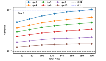
Figure 4: Frequency-domain mismatch between NR and rescaled ppBHPT waveforms using all available modes. The mismatch computation uses an advanced LIGO design sensitivity curve LIGO Scientific Collaboration (2018), an upper frequency of $4096$ Hz, and a variable lower frequency set to the (2,2) mode’s initial instantaneous frequency. We show a result for an inclination angle of 0, while non-zero inclinations are typically a factor of $\sim 1.5$ times larger. As expected, the ppBHPT and NR waveforms show better agreement at larger mass ratios.

Note that we use precisely the same $\alpha$ parameter to enact an analogous rescaling for all the higher-modes too. Since $\alpha$ has been optimized using the (2,2) mode data, the subdominant modes do not achieve relative errors as low as the (2,2) mode. Nevertheless, these higher-modes are still well modeled and the overall error, including error contributions from all modes, is nearly the same as the (2,2)-mode only error (cf. Fig. 3).

As a final test, in Fig. 4 we show a noise-weighted mismatch (cf. Eq. (22) of Ref. Blackman et al. (2017a)) between NR and the ppBHPT waveforms using all available modes. We continue to find good agreement and, as expected, as the mass ratio increases the mismatch decreases. Finally, the mismatch between our model and the new $q=15$ NR simulation (not shown) is around $.01$ for the range of total masses considered.

Summary – In this Letter we present the first surrogate model, EMRISur1dq1e4, for gravitational wave signals (including higher-order modes) from black hole binary systems over a wide range of mass-ratios. EMRISur1dq1e4 can be used to extend the banks of signal templates for LIGO/Virgo data analysis into larger mass-ratios, and also serve as a useful tool for mock data analyses for future observatories. This model is publicly available as part of both the Black Hole Perturbation Toolkit BHP and GWSurrogate Blackman et al. . Future work should include obvious extensions to the model such as spin, effects of eccentricity, and spin-orbit precession.

We also perform the first comparison between ppBHPT and NR waveforms, and find that after a rescaling of the ppBHPT’s total mass parameter there is surprisingly remarkable agreement even in the comparable mass-ratio regime. Note that the ppBHPT calculation does not incorporate any aspect of the dynamics of the background geometry within which the waves travel and nonlinearities beyond radiative corrections to the orbit. This study, which may offer some insight into the dynamics of a black hole binary system itself, is part of a growing body of evidence, initiated by Le Tiec et al. Le Tiec et al. (2011) (see also Refs. Price et al. (2011, 2013, 2016)), that suggests perturbation theory with self-force corrections are applicable to nearly equal mass systems Lewis et al. (2017); Zimmerman et al. (2016); Le Tiec et al. (2011, 2012); Le Tiec (2014); Le Tiec et al. (2013) despite there being no a priori reason to expect this should be the case. As a practical matter, our results suggest that perturbation theory with (post-)adiabatic orbital corrections may be used to generate accurate late inspiral, merger, and ringdown waveforms in the $q>10$ regime that is especially challenging for NR.

Acknowledgments – We would like to thank Alessandra Buonanno, Scott A. Hughes, Rahul Kashyap, Steve Liebling, Richard Price, Michael Pürrer, Niels Warburton, and Anil Zenginoglu for helpful feedback on this manuscript. We also thank Tousif Islam for significant assistance with porting the surrogate model to the Black Hole Perturbation Toolkit, and Matt Giesler and Mark Scheel for allowing us to use their new $q=15$ NR simulation in our study. N. R. and G. K. acknowledge research support from NSF Grants PHY-1701284 & DMS-1912716, and ONR/DURIP Grant No. N00014181255. S. E. F. is partially supported by NSF grant PHY-1806665. We also thank Scott A. Hughes for his open-source code GremlinEq, which is part of the Black Hole Perturbation Toolkit gre . This code enabled us to compute the decaying trajectories using the energy-balance approach.

References

References

- Aasi et al. (2015) J. Aasi et al. (LIGO Scientific), Class. Quant. Grav. 32, 074001 (2015), arXiv:1411.4547 [gr-qc] .
- Acernese et al. (2015) F. Acernese et al. (Virgo), Class. Quant. Grav. 32, 024001 (2015), arXiv:1408.3978 [gr-qc] .
- Abbott et al. (2016a) B. P. Abbott et al. (LIGO Scientific, Virgo), Phys. Rev. Lett. 116, 061102 (2016a), arXiv:1602.03837 [gr-qc] .
- Abbott et al. (2017a) B. P. Abbott et al. (LIGO Scientific, Virgo), Phys. Rev. Lett. 119, 161101 (2017a), arXiv:1710.05832 [gr-qc] .
- Abbott et al. (2016b) B. P. Abbott et al. (LIGO Scientific, Virgo), Phys. Rev. Lett. 116, 241103 (2016b), arXiv:1606.04855 [gr-qc] .
- Abbott et al. (2017b) B. P. Abbott et al. (LIGO Scientific, Virgo), Phys. Rev. Lett. 118, 221101 (2017b), [Erratum: Phys. Rev. Lett.121,no.12,129901(2018)], arXiv:1706.01812 [gr-qc] .
- Abbott et al. (2017c) B. P. Abbott et al. (LIGO Scientific, Virgo), Astrophys. J. 851, L35 (2017c), arXiv:1711.05578 [astro-ph.HE] .
- Abbott et al. (2017d) B. P. Abbott et al. (LIGO Scientific, Virgo), Phys. Rev. Lett. 119, 141101 (2017d), arXiv:1709.09660 [gr-qc] .
- Abbott et al. (2018a) B. P. Abbott et al. (LIGO Scientific, Virgo), (2018a), arXiv:1811.12907 [astro-ph.HE] .
- Abbott et al. (2018b) B. P. Abbott et al. (KAGRA, LIGO Scientific, VIRGO), Living Rev. Rel. 21, 3 (2018b), arXiv:1304.0670 [gr-qc] .
- Abbott et al. (2018c) B. P. Abbott et al. (LIGO Scientific, Virgo), (2018c), arXiv:1811.12940 [astro-ph.HE] .
- (12) “Ligo/virgo public alerts,” https://gracedb.ligo.org/superevents/public/O3/.
- Abbott et al. (2019) B. P. Abbott et al. (LIGO Scientific Collaboration and Virgo Collaboration), Phys. Rev. X 9, 031040 (2019).
- McKernan et al. (2019) B. McKernan, K. E. S. Ford, R. O’Shaughnessy, and D. Wysocki, “Monte-carlo simulations of black hole mergers in agn disks: Low chi effective mergers and predictions for ligo,” (2019), arXiv:1907.04356 [astro-ph.HE] .
- Hild et al. (2011) S. Hild, M. Abernathy, F. Acernese, P. Amaro-Seoane, N. Andersson, K. Arun, F. Barone, B. Barr, M. Barsuglia, M. Beker, et al., Classical and Quantum Gravity 28, 094013 (2011).
- Kalogera et al. (2019) V. Kalogera, C. P. Berry, M. Colpi, S. Fairhurst, S. Justham, I. Mandel, A. Mangiagli, M. Mapelli, C. Mills, B. Sathyaprakash, et al., arXiv preprint arXiv:1903.09220 (2019).
- Vitale and Evans (2017) S. Vitale and M. Evans, Physical Review D 95, 064052 (2017).
- Amaro-Seoane (2018) P. Amaro-Seoane, Physical Review D 98 (2018), 10.1103/physrevd.98.063018.
- Reitze et al. (2019) D. Reitze, R. X. Adhikari, S. Ballmer, B. Barish, L. Barsotti, G. Billingsley, D. A. Brown, Y. Chen, D. Coyne, R. Eisenstein, et al., arXiv preprint arXiv:1907.04833 (2019).
- Miller (2009) M. C. Miller, Classical and Quantum Gravity 26, 094031 (2009).
- Hughes (2006) S. A. Hughes, in AIP Conference Proceedings, Vol. 873 (AIP, 2006) pp. 13–20.
- Amaro-Seoane et al. (2007) P. Amaro-Seoane, J. R. Gair, M. Freitag, M. C. Miller, I. Mandel, C. J. Cutler, and S. Babak, Classical and Quantum Gravity 24, R113 (2007).
- Amaro-Seoane et al. (2017) P. Amaro-Seoane, H. Audley, S. Babak, J. Baker, E. Barausse, P. Bender, E. Berti, P. Binetruy, M. Born, D. Bortoluzzi, et al., arXiv preprint arXiv:1702.00786 (2017).
- Gair et al. (2004) J. R. Gair, L. Barack, T. Creighton, C. Cutler, S. L. Larson, E. S. Phinney, and M. Vallisneri, Classical and Quantum Gravity 21, S1595 (2004).
- Khan et al. (2018) S. Khan, K. Chatziioannou, M. Hannam, and F. Ohme, (2018), arXiv:1809.10113 [gr-qc] .
- Cotesta et al. (2018) R. Cotesta, A. Buonanno, A. Bohe, A. Taracchini, I. Hinder, and S. Ossokine, Phys. Rev. D98, 084028 (2018), arXiv:1803.10701 [gr-qc] .
- London et al. (2018) L. London, S. Khan, E. Fauchon-Jones, C. Garcia, M. Hannam, S. Husa, X. Jimenez-Forteza, C. Kalaghatgi, F. Ohme, and F. Pannarale, Phys. Rev. Lett. 120, 161102 (2018), arXiv:1708.00404 [gr-qc] .
- Pan et al. (2014) Y. Pan, A. Buonanno, A. Taracchini, L. E. Kidder, A. H. Mroue, H. P. Pfeiffer, M. A. Scheel, and B. Szilagyi, Phys. Rev. D89, 084006 (2014), arXiv:1307.6232 [gr-qc] .
- Bohe et al. (2017) A. Bohe et al., Phys. Rev. D95, 044028 (2017), arXiv:1611.03703 [gr-qc] .
- Khan et al. (2016) S. Khan, S. Husa, M. Hannam, F. Ohme, M. Purrer, X. Jimenez Forteza, and A. Bohe, Phys. Rev. D93, 044007 (2016), arXiv:1508.07253 [gr-qc] .
- Hannam et al. (2014) M. Hannam, P. Schmidt, A. Bohe, L. Haegel, S. Husa, F. Ohme, G. Pratten, and M. Purrer, Phys. Rev. Lett. 113, 151101 (2014), arXiv:1308.3271 [gr-qc] .
- Taracchini et al. (2014a) A. Taracchini et al., Phys. Rev. D89, 061502 (2014a), arXiv:1311.2544 [gr-qc] .
- Pan et al. (2011) Y. Pan, A. Buonanno, M. Boyle, L. T. Buchman, L. E. Kidder, H. P. Pfeiffer, and M. A. Scheel, Phys. Rev. D84, 124052 (2011), arXiv:1106.1021 [gr-qc] .
- Mehta et al. (2017) A. K. Mehta, C. K. Mishra, V. Varma, and P. Ajith, Phys. Rev. D96, 124010 (2017), arXiv:1708.03501 [gr-qc] .
- Babak et al. (2017) S. Babak, A. Taracchini, and A. Buonanno, Phys. Rev. D95, 024010 (2017), arXiv:1607.05661 [gr-qc] .
- Damour et al. (2013) T. Damour, A. Nagar, and S. Bernuzzi, Physical Review D 87, 084035 (2013).
- Bernuzzi and Nagar (2010) S. Bernuzzi and A. Nagar, Physical Review D 81, 084056 (2010).
- Bernuzzi et al. (2011a) S. Bernuzzi, A. Nagar, and A. Zenginoğlu, Physical Review D 83, 064010 (2011a).
- Bernuzzi et al. (2011b) S. Bernuzzi, A. Nagar, and A. Zenginoğlu, Physical Review D 84, 084026 (2011b).
- Nagar et al. (2018) A. Nagar, S. Bernuzzi, W. Del Pozzo, G. Riemenschneider, S. Akcay, G. Carullo, P. Fleig, S. Babak, K. W. Tsang, M. Colleoni, et al., Physical Review D 98, 104052 (2018).
- Taracchini et al. (2013) A. Taracchini, A. Buonanno, S. A. Hughes, and G. Khanna, Physical Review D 88, 044001 (2013).
- Taracchini et al. (2014b) A. Taracchini, A. Buonanno, G. Khanna, and S. A. Hughes, Physical Review D 90, 084025 (2014b).
- Barack and Cutler (2004) L. Barack and C. Cutler, Phys. Rev. D 69, 082005 (2004).
- Babak et al. (2007) S. Babak, H. Fang, J. R. Gair, K. Glampedakis, and S. A. Hughes, Phys. Rev. D 75, 024005 (2007).
- Chua et al. (2017) A. J. Chua, C. J. Moore, and J. R. Gair, Physical Review D 96, 044005 (2017).
- Chua and Gair (2015) A. J. K. Chua and J. R. Gair, Classical and Quantum Gravity 32, 232002 (2015).
- Field et al. (2014) S. E. Field, C. R. Galley, J. S. Hesthaven, J. Kaye, and M. Tiglio, 4, 031006 (2014), arXiv:1308.3565 [gr-qc] .
- Purrer (2014) M. Purrer, Classical and Quantum Gravity 31, 195010 (2014).
- Lackey et al. (2017) B. D. Lackey, S. Bernuzzi, C. R. Galley, J. Meidam, and C. Van Den Broeck, Phys. Rev. D95, 104036 (2017), arXiv:1610.04742 [gr-qc] .
- Doctor et al. (2017) Z. Doctor, B. Farr, D. E. Holz, and M. Purrer, Phys. Rev. D96, 123011 (2017), arXiv:1706.05408 [astro-ph.HE] .
- Blackman et al. (2015) J. Blackman, S. E. Field, C. R. Galley, B. Szilágyi, M. A. Scheel, M. Tiglio, and D. A. Hemberger, Phys. Rev. Lett. 115, 121102 (2015), arXiv:1502.07758 [gr-qc] .
- Blackman et al. (2017a) J. Blackman, S. E. Field, M. A. Scheel, C. R. Galley, D. A. Hemberger, P. Schmidt, and R. Smith, Phys. Rev. D95, 104023 (2017a), arXiv:1701.00550 [gr-qc] .
- Blackman et al. (2017b) J. Blackman, S. E. Field, M. A. Scheel, C. R. Galley, C. D. Ott, M. Boyle, L. E. Kidder, H. P. Pfeiffer, and B. Szilágyi, Phys. Rev. D96, 024058 (2017b), arXiv:1705.07089 [gr-qc] .
- Huerta et al. (2018) E. A. Huerta, C. J. Moore, P. Kumar, D. George, A. J. K. Chua, R. Haas, E. Wessel, D. Johnson, D. Glennon, A. Rebei, A. M. Holgado, J. R. Gair, and H. P. Pfeiffer, Phys. Rev. D 97, 024031 (2018), arXiv:1711.06276 [gr-qc] .
- Chua et al. (2018) A. J. Chua, C. R. Galley, and M. Vallisneri, arXiv preprint arXiv:1811.05491 (2018).
- Canizares et al. (2015) P. Canizares, S. E. Field, J. Gair, V. Raymond, R. Smith, and M. Tiglio, Phys. Rev. Lett. 114, 071104 (2015), arXiv:1404.6284 [gr-qc] .
- Galley and Schmidt (2016) C. R. Galley and P. Schmidt, (2016), arXiv:1611.07529 [gr-qc] .
- Varma et al. (2019a) V. Varma, S. E. Field, M. A. Scheel, J. Blackman, D. Gerosa, L. C. Stein, L. E. Kidder, and H. P. Pfeiffer, Phys. Rev. Research. 1, 033015 (2019a), arXiv:1905.09300 [gr-qc] .
- Varma et al. (2019b) V. Varma, S. E. Field, M. A. Scheel, J. Blackman, L. E. Kidder, and H. P. Pfeiffer, Phys. Rev. D99, 064045 (2019b), arXiv:1812.07865 [gr-qc] .
- Varma et al. (2019c) V. Varma, D. Gerosa, L. C. Stein, F. Hébert, and H. Zhang, Phys. Rev. Lett. 122, 011101 (2019c), arXiv:1809.09125 [gr-qc] .
- Lackey et al. (2019a) B. D. Lackey, M. Purrer, A. Taracchini, and S. Marsat, Physical Review D 100, 024002 (2019a).
- Lackey et al. (2019b) B. D. Lackey, M. Pürrer, A. Taracchini, and S. Marsat, Phys. Rev. D100, 024002 (2019b), arXiv:1812.08643 [gr-qc] .
- Varma and Ajith (2017) V. Varma and P. Ajith, Phys. Rev. D96, 124024 (2017), arXiv:1612.05608 [gr-qc] .
- Bustillo et al. (2018) J. C. Bustillo, J. A. Clark, P. Laguna, and D. Shoemaker, Physical review letters 121, 191102 (2018).
- Pang et al. (2018) P. T. H. Pang, J. C. Bustillo, Y. Wang, and T. G. F. Li, Phys. Rev. D 98, 024019 (2018), arXiv:1802.03306 [gr-qc] .
- Littenberg et al. (2013) T. B. Littenberg, J. G. Baker, A. Buonanno, and B. J. Kelly, Phys. Rev. D 87, 104003 (2013), arXiv:1210.0893 [gr-qc] .
- Kalaghatgi et al. (2019) C. Kalaghatgi, M. Hannam, and V. Raymond, arXiv preprint arXiv:1909.10010 (2019).
- Teukolsky (1973) S. A. Teukolsky, Astrophys. J. 185, 635 (1973).
- Sundararajan et al. (2007) P. A. Sundararajan, G. Khanna, and S. A. Hughes, Physical Review D 76, 104005 (2007).
- Sundararajan et al. (2008) P. A. Sundararajan, G. Khanna, S. A. Hughes, and S. Drasco, Physical Review D 78, 024022 (2008).
- Sundararajan et al. (2010) P. A. Sundararajan, G. Khanna, and S. A. Hughes, Physical Review D 81, 104009 (2010).
- Zenginoğlu and Khanna (2011) A. Zenginoğlu and G. Khanna, Physical Review X 1, 021017 (2011).
- Fujita and Tagoshi (2004) R. Fujita and H. Tagoshi, Progress of Theoretical Physics 112, 415 (2004), http://oup.prod.sis.lan/ptp/article-pdf/112/3/415/5382220/112-3-415.pdf .
- Fujita and Tagoshi (2005) R. Fujita and H. Tagoshi, Progress of Theoretical Physics 113, 1165 (2005), http://oup.prod.sis.lan/ptp/article-pdf/113/6/1165/5285582/113-6-1165.pdf .
- Mano et al. (1996) S. Mano, H. Suzuki, and E. Takasugi, Progress of Theoretical Physics 95, 1079 (1996), http://oup.prod.sis.lan/ptp/article-pdf/95/6/1079/5282662/95-6-1079.pdf .
- Throwe (2010) W. Throwe, High precision calculation of generic extreme mass ratio inspirals, Ph.D. thesis, Massachusetts Institute of Technology (2010).
- (77) “Black Hole Perturbation Toolkit,” (bhptoolkit.org).
- O’Sullivan and Hughes (2014) S. O’Sullivan and S. A. Hughes, “Strong-field tidal distortions of rotating black holes: Formalism and results for circular, equatorial orbits,” (2014), arXiv:1407.6983 [gr-qc] .
- Drasco and Hughes (2006) S. Drasco and S. A. Hughes, Physical Review D 73 (2006), 10.1103/physrevd.73.024027.
- Ori and Thorne (2000) A. Ori and K. S. Thorne, Physical Review D 62, 124022 (2000).
- Hughes et al. (2019) S. A. Hughes, A. Apte, G. Khanna, and H. Lim, arXiv preprint arXiv:1901.05900 (2019).
- Apte and Hughes (2019) A. Apte and S. A. Hughes, “Exciting black hole modes via misaligned coalescences: I. inspiral, transition, and plunge trajectories using a generalized ori-thorne procedure,” (2019), arXiv:1901.05901 [gr-qc] .
- Hinderer and Flanagan (2008) T. Hinderer and Ã. Ã. Flanagan, Physical Review D 78 (2008), 10.1103/physrevd.78.064028.
- Gralla (2012) S. E. Gralla, Physical Review D 85 (2012), 10.1103/physrevd.85.124011.
- Pound (2012) A. Pound, Physical Review Letters 109 (2012), 10.1103/physrevlett.109.051101.
- Pound et al. (2019) A. Pound, B. Wardell, N. Warburton, and J. Miller, “Second-order self-force calculation of gravitational binding energy,” (2019), arXiv:1908.07419 [gr-qc] .
- McKennon et al. (2012) J. McKennon, G. Forrester, and G. Khanna, in Proceedings of the 1st Conference of the Extreme Science and Engineering Discovery Environment: Bridging from the eXtreme to the campus and beyond (ACM, 2012) p. 14.
- Maday et al. (2009) Y. Maday, N. C. Nguyen, A. T. Patera, and S. H. Pau, Communications on Pure and Applied Analysis 8, 383 (2009).
- Chaturantabut and Sorensen (2010) S. Chaturantabut and D. C. Sorensen, SIAM Journal on Scientific Computing 32, 2737 (2010).
- Blackman et al. (2017c) J. Blackman, S. E. Field, M. A. Scheel, C. R. Galley, D. A. Hemberger, P. Schmidt, and R. Smith, Physical Review D 95, 104023 (2017c).
- Barausse et al. (2012) E. Barausse, A. Buonanno, S. A. Hughes, G. Khanna, S. O’Sullivan, and Y. Pan, Physical Review D 85, 024046 (2012).
- Boyle et al. (2007) M. Boyle, D. A. Brown, L. E. Kidder, A. H. Mroue, H. P. Pfeiffer, M. A. Scheel, G. B. Cook, and S. A. Teukolsky, Phys. Rev. D76, 124038 (2007), arXiv:0710.0158 [gr-qc] .
- Boyle et al. (2019) M. Boyle, D. Hemberger, D. A. Iozzo, G. Lovelace, S. Ossokine, H. P. Pfeiffer, M. A. Scheel, L. C. Stein, C. J. Woodford, A. B. Zimmerman, et al., arXiv preprint arXiv:1904.04831 (2019).
- (94) SXS Collaboration, “The SXS collaboration catalog of gravitational waveforms,” http://www.black-holes.org/waveforms.
- Mroue et al. (2013) A. H. Mroue et al., Phys. Rev. Lett. 111, 241104 (2013), arXiv:1304.6077 [gr-qc] .
- Giesler et al. (2020) M. Giesler, M. Scheel, and V. Varma, in prep (2020).
- Varma et al. (2020) V. Varma, M. Giesler, and M. Scheel, in prep (2020).
- LIGO Scientific Collaboration (2018) LIGO Scientific Collaboration, Updated Advanced LIGO sensitivity design curve, Tech. Rep. (2018) https://dcc.ligo.org/LIGO-T1800044/public.
- (99) “Black Hole Perturbation Toolkit,” (bhptoolkit.org).
- (100) J. Blackman, S. Field, C. Galley, and V. Varma, “gwsurrogate,” https://pypi.python.org/pypi/gwsurrogate/.
- Le Tiec et al. (2011) A. Le Tiec, A. H. Mroue, L. Barack, A. Buonanno, H. P. Pfeiffer, N. Sago, and A. Taracchini, Physical review letters 107, 141101 (2011).
- Price et al. (2011) R. H. Price, G. Khanna, and S. A. Hughes, Physical Review D 83, 124002 (2011).
- Price et al. (2013) R. H. Price, G. Khanna, and S. A. Hughes, Physical Review D 88, 104004 (2013).
- Price et al. (2016) R. H. Price, S. Nampalliwar, and G. Khanna, Physical Review D 93, 044060 (2016).
- Lewis et al. (2017) A. G. Lewis, A. Zimmerman, and H. P. Pfeiffer, Classical and Quantum Gravity 34, 124001 (2017).
- Zimmerman et al. (2016) A. Zimmerman, A. G. Lewis, and H. P. Pfeiffer, Physical review letters 117, 191101 (2016).
- Le Tiec et al. (2012) A. Le Tiec, E. Barausse, and A. Buonanno, Physical review letters 108, 131103 (2012).
- Le Tiec (2014) A. Le Tiec, International Journal of Modern Physics D 23, 1430022 (2014).
- Le Tiec et al. (2013) A. Le Tiec, A. Buonanno, A. H. Mroue, H. P. Pfeiffer, D. A. Hemberger, G. Lovelace, L. E. Kidder, M. A. Scheel, B. Szilágyi, N. W. Taylor, et al., Physical Review D 88, 124027 (2013).