Electron spin resonance in spiral antiferromagnet linarite: theory and experiment

Abstract

We present combined experimental and theoretical investigation of the low-frequency ESR dynamics in the ordered phases of magnetic mineral linarite. This material consists of weakly coupled spin-1/2 chains of copper ions with frustrated ferro- and antiferromagnetic interactions. In zero magnetic field, linarite orders into a spiral structure and exhibits a peculiar magnetic phase diagram sensitive to the field orientation. The resonance frequencies and their field dependence are analyzed combining microscopic and macroscopic theoretical approaches and precise values of magnetic anisotropy constants are obtained. We conclude that possible realization of exotic multipolar quantum states in this material is greatly influenced by the biaxial anisotropy.

I Introduction

The frustrated spin-1/2 chain model with nearest neighbor ferromagnetic $J_{1}<0$ and next-nearest neighbor antiferromagnetic $J_{2}>0$ exchanges has recently attracted a great deal of interest owing to its exotic quantum properties. In strong magnetic fields the model can exhibit the longitudinal spin-density wave, the spin nematic, and even higher-order multipolar phases Chubukov91 ; Heidrich06 ; Kecke07 ; Hikihara08 ; Sudan09 ; Heidrich09 ; Shindou09 ; Zhitomirsky10 ; Nishimoto15 . Frustrated ferromagnetic chains are realized in a family of copper-oxide materials with edge-sharing CuO₂ plaquettes represented, for instance, by LiCuVO₄ Gibson04 ; Enderle05 , Rb₂Cu₂Mo₃O₁₂ Hase_2004 , LiCu₂O₂ Matsuda_2004 , NaCu₂O₂ Drechsler_2006 , Li₂ZrCuO₄ Drechsler_2007 and PbCuSO₄(OH)₂ (linarite) Baran_2006 . Among these the natural mineral linarite PbCuSO₄(OH)₂ Baran_2006 ; Yasui_2011 ; Willenberg_2012 ; Wolter_2012 ; Schapers_2013 ; Willenberg_2016 ; Povarov_2016 ; Rule_2017 ; Cemal_2018 ; Feng18 ; Heinze19 combines a moderate saturation field of about 10 T with close proximity to the quantum critical point $|J_{2}/J_{1}|_{c}=1/4$, which may provide direct access to the most exotic multipolar states Hikihara08 . Besides that, linarite exhibits a unique phase diagram for magnetic fields applied along the chain direction with up to five commensurate and incommensurate phases Willenberg_2012 ; Willenberg_2016 ; Feng18 .

There is an ongoing debate on the role of anisotropy for the observed properties of linarite Cemal_2018 ; Feng18 ; Heinze19 . Indeed, the phase diagram changes dramatically once magnetic field is tilted away from the chain direction. Cemal et al. Cemal_2018 have suggested the minimal anisotropic model with orthorhombic symmetry and estimated corresponding microscopic parameters for linarite on the basis of the inelastic neutron scattering measurements in the high-field polarized phase. Here, we present our experimental results on the low-frequency dynamics in linarite studied by the electron spin resonance (ESR) technique together with theoretical analysis based on the microscopic model as well as on the phenomenological hydrodynamic theory. The main advantage of the ESR method for studying the anisotropy effects is its high frequency/energy resolution, which allows us to obtain much more reliable values of the anisotropy constants. In the remaining part of Introduction we review the basic crystallographic and magnetic properties of linarite that are important for our subsequent analysis.

The crystal lattice of linarite belongs to the monoclinic space group $P2_{1}/m$ with lattice parameters $a=9.70$ Å, $b=5.65$ Å, $c=4.69$ Å, and $\beta=102.7^{\circ}$ Effenberger_1987 . Figure 1 shows a schematic crystal structure including only Cu²⁺ ions. The CuO₂ plaquettes form weakly pleated ribbons and the crystal unit cell contains two adjacent copper ions along the $b$ axis. Still, from the point of view of isotropic exchange interactions, the copper chains remain uniform with the same exchange coupling $J_{1}$ in all spin pairs at distance $b/2$ and $J_{2}$ for second nearest neighbors at distance $b$. In zero field, linarite magnetically orders at $T_{N}\approx 2.8$ K into an elliptic spiral structure with the propagation vector ${\bf k}_{ic}=(0,0.189,1/2)$ in the reciprocal lattice units Willenberg_2012 . The spin spiral rotates in the $xy$ plane, where the $y$ axis is parallel to the crystallographic $b$ axis and the $x$ axis lies in the $ac$ plane making an angle 27^∘ with the $a$ axis. Two components of the order parameter in this elliptic spiral state are $\mu_{x}\approx 0.64~{}\mu_{B}$ and $\mu_{y}\approx 0.83~{}\mu_{B}$ Willenberg_2012 .

In applied field, linarite exhibits a variety of magnetic structures depending on field strength and orientation, see Fig. 1. Magnetic phases and transition fields presented in Fig. 1 are given in accordance with Refs. Cemal_2018 ; Povarov_2016 . For magnetic field applied parallel to the spiral plane along the easy $x$ axis, the observed phase sequence, spin helix — spin cone — spin fan, conforms to the one expected for magnetic spirals in the presence of anisotropy Nagamiya67 . For the orthogonal in-plane direction ${\bf H}\parallel{\bf b}$, an additional commensurate phase characterized by ${\bf k}_{c}=(0,0,1/2)$ appears instead of the conical state in a wide range of fields. Its presence has been attributed to the biaxial anisotropy, which competes with an incommensurate tendency set by competing exchanges Cemal_2018 . Common to all field directions is the fan phase stabilized in the vicinity of the transition into the polarized state as expected on general symmetry arguments Nagamiya67 . An alternative scenario put forward in Willenberg_2016 identifies the high-field phase with the longitudinal spin-density wave (SDW) characteristic to one-dimensional $J_{1}$–$J_{2}$ chains. Such a suggestion is motivated by observation of a peculiar field/temperature dependence of the ordering wave vector in high fields. However, Cemal et al. Cemal_2018 have subsequently shown that the nontrivial field dependence $k_{ic}(H)$ at the lowest temperature $T=60$ mK is at least partially accounted for by the effect of magnetic anisotropy in the fan phase. In any case, at the transition to the saturated phase the ordering wave vector $k_{ic}$ remains finite in linarite Willenberg_2016 ; Cemal_2018 in contradiction to the SDW scenario, which predicts $k_{ic}\to 0$.

The recent high-field NMR measurements for ${\bf H}\parallel{\bf b}$ leave a narrow window of fields 9.35 T $\leq H\leq 9.64$ T, where a spin nematic phase may be present in linarite Heinze19 . A rather small field region for the exotic quantum phase is not entirely surprising in view of relatively large ordered moments in this material in zero magnetic field and, consequently, small quantum fluctuations. In contrast, LiCuVO₄, another candidate material for the high-field nematic phase Svistov11 ; Orlova17 , has notably smaller moments $\sim 0.3\mu_{B}$ Gibson04 making it a more feasible venue for observing exotic quantum physics albeit in higher magnetic fields. Note, that even in the absence of the multipolar quantum states the phase diagram of linarite provides an interesting example of an incommensurate magnet under combined effect of anisotropy and magnetic field Nagamiya67 .

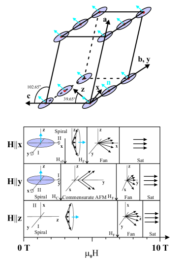
Figure 1: (Color online.) Upper panel: Schematic crystal structure of linarite showing the positions of magnetic copper ions (small red circles). The spiral magnetic structure in zero field is illustrated by grey ellipses. The orthogonal triad $\hat{\bf x},\hat{\bf y},\hat{\bf z}$ marks the principal axes of the anisotropy tensor. The hard axis $\hat{\bf z}$ is perpendicular to the spiral plane, whereas the intermediate axis $\hat{\bf y}\parallel{\bf b}$. Bottom panel: Magnetic structures appearing for different orientations of an external field for $T=1.3$ K.

The paper is organized as follows. In Section II we provide the theoretical basis for interpreting the low-frequency ESR dynamics using both the microscopic spin-wave approach (Sec. IIA) and the macroscopic field-theoretical treatment (Sec. IIB). Section III describes experimental results that are compared to the theoretical predictions. In Sec. IV we conclude by emphasizing the main consequences to the physics of linarite.

II Theory

II.1 Spin Model

In accordance with the monoclinic symmetry of linarite crystals, we base our theoretical consideration on a general anisotropic exchange Hamiltonian for spins $S=1/2$ written in the global coordinate frame as

$$\hat{\cal H}=\sum_{\langle ij\rangle}\bigl{[}J_{ij}^{xx}S_{i}^{x}S_{j}^{x}+J_{ij}^{yy}S_{i}^{y}S_{j}^{y}+J_{ij}^{zz}S_{i}^{z}S_{j}^{z}\bigr{]},$$ (1)

where $\hat{\bf y}$ is chosen along the two-fold $b$ axis and $\hat{\bf x}$ and $\hat{\bf z}$ are oriented in the $ac$ plane. The Hamiltonian (1) provides the minimal anisotropic spin model for linarite. In particular, we assume that principal axes of the symmetric exchange tensor are the same for each bond, which is generally not true. However, as we shall see below, the exchange anisotropies contribute additively to the ESR gaps. Therefore, in the case of a large difference between exchange bonds, one can take into account the anisotropy of the strongest bond only. Also, the pleated structure of the CuO₂ ribbons in linarite allows for the antisymmetric Dzyaloshinskii-Moriya (DM) interaction on the nearest-neighbor bonds. We omit this interaction in the minimal model since (i) due to staggering of the DM vectors it does not affect the pitch angle of the spin spiral and (ii) the inelastic neutron scattering (INS) measurements Rule_2017 ; Cemal_2018 successfully fit the magnon dispersion data without the DM term.

There is an emergent consensus in literature that magnetic properties of linarite are determined by competing ferromagnetic nearest-neighbor $J_{1}$ and antiferromagnetic second-neighbor $J_{2}$ exchanges inside the spin chains as well as by an interchain coupling $J_{ic}$. Still, different authors proposed quite different values of the microscopic parameters, see Table 1, where we also indicated the experimental techniques used in each study. An accurate estimate of the exchange parameters of linarite was obtained by the INS measurements in high magnetic fields Cemal_2018 , which suppress quantum fluctuations. In the same work, the dominant interchain coupling was identified as $J_{c}$, exchange between nearest neighbors in the $c$ direction. In contrast, the zero-field neutron measurements Rule_2017 suggested a dominant diagonal interchain coupling $J_{c}^{\prime}$ (quoted in Table 1). This conclusion was based on the spin-wave fits of the low-energy part of the spectrum, where according to the dynamical DMRG simulations Sirker12 quantum renormalization effects are significant and the harmonic spin-wave theory is poorly applicable.

Table 1: Microscopic exchange constants of linarite from different works together with the computed ratio of magnetic susceptibilities using Eqs. (24) and (28). The last two rows give $\chi_{\perp}/\chi_{\parallel}$ measured experimentally Yasui_2011 or directly derived from our ESR data.

Method	$J_{1}$ [K]	$J_{2}$ [K]	$J_{ic}$ [K]	$\chi_{\perp}/\chi_{\parallel}$
$\chi(T)$ Yasui_2011	$-13\pm 3$	$21\pm 5$	$-$	$2.7$
$M(H)$, $\chi(T)$ Wolter_2012	$-100$	36	$-$	$6.7$
INS ($H=0$) Rule_2017
LSWT	$-114\pm 2$	$37\pm 1$	$4\pm 0.5$	2.2
DMRG	$-78$	$28$	$7$	1.7
INS ($H>H_{\rm sat}$) Cemal_2018	$-168$	$46$	$8$	2.2
$M(H)$, $T=2$ K Yasui_2011				$1.6\pm 0.1$
ESR, $T=1.3$ K				$1.85\pm 0.1$
(this study)

In the rest of the article, both $J_{2}$ and $J_{c}$ are assumed to be isotropic, whereas the biaxial anisotropy of the ferromagnetic nearest-neighbor bonds is represented as

$$\hat{\cal H}=J_{1}\sum_{\langle ij\rangle}\bigl{[}(1+\varepsilon)S_{i}^{x}S_{j}^{x}+(1-\varepsilon)S_{i}^{y}S_{j}^{y}+(1-\delta)S_{i}^{z}S_{j}^{z}\bigr{]}$$ (2)

with $0<\varepsilon<\delta$ such that $x$ and $z$ are the easy and the hard axis, respectively. The same choice of axes was adopted by Cemal et al. Cemal_2018 , though our definitions of $\delta$ and $\varepsilon$ are somewhat different.

II.2 Microscopic Theory

The spin-wave theory of incommensurate helical magnetic structures was developed by various authors in the sixties Cooper62 ; Cooper63 ; Elliot66 ; Nagamiya67 ; Cooper68 , see also recent works Zhitomirsky96 ; Chen13 ; Milstein15 . The motivation for the early studies was chiefly from the experimental investigation of rare-earth compounds dominated by the single-ion anisotropy. In this section, we extend the previous analysis to the case of the symmetric exchange anisotropy relevant for Kramers ions with an effective spin $S=1/2$ and provide a few additional results.

II.2.1 Zero magnetic field

We assume that competing exchange interactions produce a spiral spin structure in the $xy$ plane. The first standard step consists in transformation from the fixed global frame to the rotating local coordinate axes $(x_{i},y_{i},z_{i})$ such that $\hat{\bf z}_{i}$ is always oriented along the equilibrium spin direction on a given site $i$ and $\hat{\bf y}_{i}$ is orthogonal to the plane of the spiral. Spin components in the global frame (denoted below by $0$ subscripts) are related to those in the rotating local frame by

$$S_{i}^{x_{0}}=S_{i}^{z}\cos\theta_{i}-S_{i}^{x}\sin\theta_{i}\,,$$ (3)

$$S_{i}^{y_{0}}=S_{i}^{z}\sin\theta_{i}+S_{i}^{x}\cos\theta_{i}\,,\quad S_{i}^{z_{0}}=S_{i}^{y}\,,$$

where $\theta_{i}$ is the rotation angle to be determined later. It is convenient to introduce

$$J_{ij}=\frac{1}{2}\bigl{(}J_{ij}^{xx}+J_{ij}^{yy}\bigr{)}\,,\quad\varepsilon_{ij}=\frac{1}{2}\bigl{(}J_{ij}^{xx}-J_{ij}^{yy}\bigr{)}\,.$$ (4)

The Hamiltonian (1) written in the local frame becomes

$$\hat{\cal H} = \sum_{\langle ij\rangle}\Bigl{[}J_{ij}\cos(\theta_{i}-\theta_{j})(S_{i}^{z}S_{j}^{z}+S_{i}^{x}S_{j}^{x})+J_{ij}^{zz}S_{i}^{y}S_{j}^{y}$$ (5)

$$\mbox{}+\varepsilon_{ij}\cos(\theta_{i}+\theta_{j})(S_{i}^{z}S_{j}^{z}-S_{i}^{x}S_{j}^{x})+\ldots\Bigr{]},$$

In the above expression we dropped mixed terms like $S_{i}^{z}S_{j}^{x}$ since those play no role in the following calculations.

Zero-temperature classical energy is obtained from Eq. (5) by neglecting all fluctuations, $S_{i}^{z}\to S$, $S_{i}^{x,y}\to 0$,

$$E_{\rm cl}=S^{2}\sum_{\langle ij\rangle}\bigr{[}J_{ij}\cos(\theta_{i}-\theta_{j})+\varepsilon_{ij}\cos(\theta_{i}+\theta_{j})\bigr{]}.$$ (6)

For uniaxial planar anisotropy ($\varepsilon_{ij}=0$), spins rotate uniformly in space by $\theta_{i}={\bf Q}\cdot{\bf r}_{i}$, where $\bf Q$ corresponds to the minimum of the Fourier transform

$$J_{\bf q}=\sum_{j}J_{ij}\,e^{i{\bf q}({\bf r}_{i}-{\bf r}_{j})}\ .$$ (7)

For the microscopic model of linarite we have

$$J_{\bf q}=-2|J_{1}|\cos q_{y}+2J_{2}\cos 2q_{y}+2J_{c}\cos q_{z}\ ,$$ (8)

where we set all nearest-neighbor distances to 1. The minimum is achieved for ${\bf Q}=(0,Q,\pi)$ with

$$\cos Q=\frac{|J_{1}|}{4J_{2}}\ .$$ (9)

A sizeable second-neighbor exchange $J_{2}\sim 0.3|J_{1}|$ produces the incommensurate spin spiral along the copper chains, whereas $J_{c}>0$ is responsible for antiferromagnetic spin arrangement between chains in the $c$ direction.

The in-plane anisotropy $\varepsilon_{ij}\neq 0$ distorts uniform rotation of spins in space Nagamiya67 ; Zhitomirsky96

$$\theta_{i}={\bf Q}\cdot{\bf r}_{i}+\varphi_{i}\ ,\ \ \ \varphi_{i}=\varphi\sin(2{\bf Q}{\bf r}_{i})\ .$$ (10)

Minimization of (6) with respect to $\varphi$ yields to the leading order in small $\varepsilon_{ij}$:

$$\varphi=\frac{2\varepsilon_{\bf Q}}{J_{3\bf Q}-J_{\bf Q}}\ ,$$ (11)

where $\varepsilon_{\bf Q}=\sum_{j}\varepsilon_{ij}\,e^{i{\bf Qr}_{ij}}$. Spins bunch towards the easy direction in the $xy$ plane producing satellite Bragg peaks at ${\bf q}=\pm 3{\bf Q}$ alongside with the principal peaks at ${\bf q}=\pm{\bf Q}$. The spin bunching also results in an elliptical distortion of the spiral:

$$\frac{\langle S^{x_{0}}_{\bf Q}\rangle}{\langle S^{y_{0}}_{\bf Q}\rangle}=\frac{1-d}{1+d}\ ,\ \ \ d=\frac{\varepsilon_{\bf Q}}{J_{3\bf Q}-J_{\bf Q}}\ .$$ (12)

The experimental value $d\approx 0.13$ for linarite Willenberg_2012 can be straightforwardly related to the parameters of the model (2). Using $\varepsilon_{\bf Q}=-2\varepsilon|J_{1}|\cos Q$ and $J_{3\bf Q}-J_{\bf Q}=8|J_{1}|\sin^{3}\!Q\sin 2Q$ with the exchange parameters derived by Cemal et al. Cemal_2018 we obtain $d\approx 5.6\varepsilon$ that gives an estimate $\varepsilon\sim 0.02$. This value of $\varepsilon$ is about 3 times larger than a more precise estimate derived from the ESR measurements in Sec. III.2. For more accurate determination of $\varepsilon$ from ellipticity of the magnetic structure one may resort to numerical real-space simulations described in Cemal_2018 ; Gvozdikova16 .

The excitation spectra are computed in the harmonic approximation neglecting quantum corrections. For that we use the truncated Holstein-Primakoff transformation for spin components in the local frame: $S_{i}^{z}=S-a_{i}^{\dagger}a_{i}$, $S_{i}^{x}\approx\sqrt{S/2}\,(a_{i}^{\dagger}+a_{i})$, and $S_{i}^{y}\approx i\sqrt{S/2}\,(a_{i}^{\dagger}-a_{i})$. Substituting it into Eq. (5) and keeping only quadratic terms in boson operators we obtain the harmonic spin-wave Hamiltonian $\hat{\cal H}_{2}$. After the Fourier transformation and expansion in small $\varphi_{i}$, $\hat{\cal H}_{2}$ takes the following form:

$$\hat{\cal H}_{2} = \sum_{\bf k}\Bigl{[}A_{\bf k}a^{\dagger}_{\bf k}a_{\bf k}-\frac{1}{2}\,B_{\bf k}(a_{\bf k}a_{-\bf k}+a_{-\bf k}^{\dagger}a^{\dagger}_{\bf k})$$

$$+ C_{\bf k}(a^{\dagger}_{\bf k+Q}a_{\bf k-Q}+a^{\dagger}_{\bf k-Q}a_{\bf k+Q})$$

$$+ \frac{1}{2}\,D_{\bf k}(a_{\bf k+Q}a_{\bf-k+Q}+a_{\bf k-Q}a_{\bf-k-Q}+\textrm{h.c.})\Bigr{]},$$

where

$$A_{\bf k} = \frac{S}{2}J^{zz}_{\bf k}+\frac{S}{4}(J_{\bf k+Q}+J_{\bf k-Q})-SJ_{\bf Q}\,,$$ (14)

$$B_{\bf k} = \frac{S}{2}J^{zz}_{\bf k}-\frac{S}{4}(J_{\bf k+Q}+J_{\bf k-Q})\,,\ \ C_{\bf k}=D_{\bf k}-\varepsilon_{\bf Q}S\,,$$

$$D_{\bf k} = -\frac{S}{4}\Bigl{\{}\varepsilon_{\bf k}+\varphi\Bigl{[}J_{\bf k}-\frac{1}{2}(J_{{\bf k}+2{\bf Q}}+J_{{\bf k}-2{\bf Q}})\Bigr{]}\Bigr{\}}.$$

The last two terms in (II.2.1) vanish for the uniaxial symmetry, $\varepsilon_{ij}\equiv 0$. In this case, $\hat{\cal H}_{2}$ is diagonalized by the standard Bogolyubov transformation, which eliminates the anomalous terms. The magnon energy is, then, expressed as

$$\epsilon_{\bf k}=\sqrt{A_{\bf k}^{2}-B^{2}_{\bf k}}$$ (15)

with $A_{\bf k}$, $B_{\bf k}$ taken from (14).

Using the ESR technique, one can measure magnetic excitations for only a few selected momenta. The oscillating radio-frequency (rf) field in ESR experiments is uniform within a sample:

$$\hat{V}(t)=-\sum_{i}{\bf h}(t)\cdot{\bf S}_{i}\,.$$ (16)

Rewritten in the rotating frame (3), $\hat{V}(t)$ becomes

$$\hat{V}=-\!\sum_{i}\bigl{\{}h_{y}(t)S^{y}_{i}+\bigl{[}h_{x}(t)\cos{\bf Qr}_{i}\!-h_{z}(t)\sin{\bf Qr}_{i}\bigr{]}S^{x}_{i}\bigr{\}},$$ (17)

where we keep only transverse spin components and set $\varphi_{i}=0$ (10) for simplicity. Equation (17) shows that an rf field couples to magnetic excitations with ${\bf k}=0$ and $\pm{\bf Q}$ and its polarization determines relative intensity of absorption lines. For a uniform spin spiral, magnon with ${\bf k}=0$ has vanishing energy and the resonance spectrum in zero field consists of two degenerate frequencies corresponding to ${\bf k}=\pm{\bf Q}$ magnons

$$\Delta_{0}=S\sqrt{(J_{\bf Q}^{zz}-J_{\bf Q})\bigl{[}{\textstyle\frac{1}{2}}(J_{0}+J_{2\bf Q})-J_{\bf Q}\bigr{]}}\ .$$ (18)

Considering now a general case, we note that the additional terms determined by the in-plane anisotropy mix a spin wave propagating with momentum $\bf k$ with two other magnons at momenta ${\bf k}\pm 2{\bf Q}$, which in turn are coupled to excitations with ${\bf k}\pm 4{\bf Q}$ and so on. Calculation of normal modes requires in the case diagonalization of infinite matrices for incommensurate $\bf Q$. Following Zhitomirsky96 , we adopt an approximate method for determining the ESR frequencies. First, for an incommensurate spiral the ${\bf k}=0$ magnon has zero energy even in the presence of mixing terms. The gapless nature of this mode follows from an arbitrary choice of the phase of the incommensurate spiral Elliot66 . Second, we aim to compute the ESR gaps or, more precisely, $\Delta^{2}$ including $O(\varepsilon)$ contributions. In this case, the coupling between ${\bf k}=\pm{\bf Q}$ magnons and excitations with ${\bf k}=\pm{3\bf Q}$ can be neglected. The remaining bosonic terms in (II.2.1) are

$$\hat{\cal H}^{\prime}_{2}=A_{\bf Q}(a^{\dagger}_{\bf Q}a_{\bf Q}+a^{\dagger}_{-\bf Q}a_{-\bf Q})-B_{\bf Q}(a_{\bf Q}a_{\bf-Q}+a^{\dagger}_{\bf-Q}a^{\dagger}_{\bf Q})$$

$$\mbox{}+C_{0}(a^{\dagger}_{\bf Q}a_{\bf-Q}+a^{\dagger}_{-\bf Q}a_{\bf Q})+\frac{1}{2}D_{0}(a_{\bf Q}^{2}+a_{\bf-Q}^{2}+\textrm{h.c.}).$$ (19)

This quadratic form is diagonalized by introducing symmetric/antisymmetric combinations $a_{1,2}=(a_{\bf Q}\pm a_{\bf-Q})/\sqrt{2}$, which decouple from each other, and the subsequent Bogolyubov transformation. The obtained energies are

$$\Delta_{1,2}^{2}=(A_{\bf Q}\pm C_{0})^{2}-(B_{\bf Q}\mp D_{0})^{2}\ .$$ (20)

Substituting now expressions (14) and keeping only $O(\varepsilon)$ terms we can express the ESR frequencies as

$$\Delta_{1} = S\sqrt{(J_{\bf Q}^{zz}-J^{xx}_{\bf Q})\bigl{[}{\textstyle\frac{1}{2}}(J_{0}+J_{2\bf Q})-J_{\bf Q}\bigr{]}}\ ,$$

$$\Delta_{2} = S\sqrt{(J_{\bf Q}^{zz}-J^{yy}_{\bf Q})\bigl{[}{\textstyle\frac{1}{2}}(J_{0}+J_{2\bf Q})-J_{\bf Q}\bigr{]}}\ .$$ (21)

The splitting between two ESR modes provides a direct measure of the in-plane anisotropy. In the case of linarite we have

$$\frac{\Delta_{1}}{\Delta_{2}}=\sqrt{\frac{J_{1}^{xx}-J_{1}^{zz}}{J_{1}^{yy}-J_{1}^{zz}}}=\sqrt{\frac{\delta+\varepsilon}{\delta-\varepsilon}}\ ,$$ (22)

which is directly used in Sec. III.2 for determining $\delta/\varepsilon$ from the experimental data.

II.2.2 Finite magnetic fields

We write the Zeeman energy in the form

$$\hat{\cal H}_{Z}=-{\bf H}\cdot\sum_{i}{\bf S}_{i}$$ (23)

rescaling magnetic field components with the principal values of the anisotropic $g$ tensor. By doing that we neglect a possible staggered component of the $g$-tensors of copper ions, which is compatible with the pleated structure of CuO₄ ribbons. Let us begin with the case of magnetic field oriented perpendicular to the helical plane. Spins form a conical structure, which is especially simple for vanishing in-plane anisotropy: spins tilt towards the field direction preserving uniform rotation inside the plane. The details of corresponding calculations can be found, for example, in Zhitomirsky96 . Here we present only the final results. The magnetic susceptibility per spin is given by

$$\chi_{\perp}=\frac{1}{(J_{0}-J_{\bf Q})}\ .$$ (24)

Diagonalizing the harmonic spin-wave Hamiltonian one can obtain an analytic expression for the magnon energy in the entire Brillouin zone. One of the ESR frequencies corresponding to the ${\bf k}=0$ magnon remains equal to zero, whereas two other gaps are

$$\Delta_{1,2}=\sqrt{\Delta_{0}^{2}+H^{2}\frac{[\frac{1}{2}(J_{0}\!+\!J_{2\bf Q})-J_{\bf Q}]^{2}}{(J_{0}-J_{\bf Q})^{2}}}\pm\frac{H}{2}\frac{J_{0}-J_{2\bf Q}}{J_{0}-J_{\bf Q}},$$ (25)

where $\Delta_{0}$ is given by (18).

Magnetic field applied parallel to the helix plane distorts uniform rotation of spins in space:

$$\theta_{i}={\bf Q}\cdot{\bf r}_{i}-\alpha_{i}\ .$$ (26)

To the first order in small $H$, the spiral distortion is expressed as Cooper63 ; Zhitomirsky96

$$\alpha_{i}=\alpha\sin({\bf Q}{\bf r}_{i})\ ,\quad\alpha=\frac{H}{S[\frac{1}{2}(J_{0}+J_{2\bf Q})-J_{\bf Q}]}\ .$$ (27)

Accordingly, the magnetic susceptibility is

$$\chi_{\parallel}=\frac{1}{(J_{0}+J_{2\bf Q}-2J_{\bf Q})}\ .$$ (28)

An important characteristic of a spin helix is anisotropy of the susceptibility tensor $\chi_{\perp}/\chi_{\parallel}$ or

$$\eta=\frac{\chi_{\perp}-\chi_{\parallel}}{\chi_{\parallel}}=\frac{J_{2\bf Q}-J_{\bf Q}}{J_{0}-J_{\bf Q}}\ .$$ (29)

Generally, one has $\eta>0$ or $\chi_{\perp}/\chi_{\parallel}>1$, since $\bf Q$ corresponds to the minimum of the Fourier transform $J_{\bf q}$ (7). In particular, this means that in the absence of anisotropy, the helical plane is oriented perpendicular to the applied magnetic field. Values of $\chi_{\perp}/\chi_{\parallel}$ computed for different sets of the exchange parameters are shown in Table 1 remark .

Calculation of the ESR frequencies from the spin-wave theory becomes rather cumbersome for magnetic field applied in the plane of spin helix Cooper63 . Instead, in the next subsection we present a simple derivation of the corresponding ESR spectra within the framework of the macroscopic field-theoretical approach.

The special feature of the phase diagram of linarite is presence of a commensurate canted antiferromagnetic state for a magnetic field applied parallel to the intermediate $y$ axis Willenberg_2016 . This two-sublattice state is described by the propagation vector ${\bf Q}_{0}=(0,0,\pi)$ and appears due competition between incommensuration and the in-plane anisotropy Cemal_2018 . Computation of the excitation spectra within the harmonic spin-wave theory is straightforward for this state. The two ESR frequencies corresponding to magnons with ${\bf k}=0$ and ${\bf k}={\bf Q}_{0}$ are

$$\Delta_{1} = 2|J_{1}|S\sqrt{(2j_{c}+\delta+\varepsilon)(2j_{c}\sin^{2}\beta+\delta\cos^{2}\beta)}\ ,$$

$$\Delta_{2} = 2|J_{1}|S\sqrt{(\delta+\varepsilon)(2j_{c}+\delta)}\cos\beta\ ,$$ (30)

where $j_{c}=J_{c}/|J_{1}|$ and $\beta$ is the canting angle:

$$\sin\beta=\frac{H}{2S|J_{1}|(\delta+2j_{c})}\,.$$

Comparison of the experimental values of the ESR gap in the commensurate state to the theoretical expressions (30) provides another consistency check for different sets of microscopic parameters for linarite.

II.3 Macroscopic Theory

An alternative prospective on the ESR spectra of ordered and disordered magnets is provided by the macroscopic or hydrodynamic theory of magnetization dynamics. This field-theoretical approach was developed by several authors Halperin69 ; Halperin77 ; Andreev80 ; Affleck89 , who applied it to both ordered and disordered magnetic phases. The main idea is to ‘integrate out’ the high-energy excitations and focus exclusively on the long-wavelength, low-energy modes. The long-wavelength oscillations only weakly perturb an underlying magnetic structure. Therefore, one can introduce a local antiferromagnetic order parameter and investigate its dynamics using the gradient expansion. For dominant exchange interactions, the emergent energy functional or Lagrangian has a universal form. For a collinear Heisenberg antiferromagnet it coincides with that for the nonlinear $\sigma$-model Andreev80 ; Affleck89 . In the subsequent analysis we follow the formulation by Andreev and Marchenko Andreev80 , who specifically considered the ESR dynamics of ordered antiferromagnets.

The staggered magnetization of a spiral antiferromagnet formed by competing exchange interactions is described by a pair of orthogonal unit vectors ${\bf l}_{1}$ and ${\bf l}_{2}$ that determine the helix plane:

$$\langle{\bf S}_{i}\rangle\simeq{\bf l}_{1}\cos{\bf Qr}_{i}+{\bf l}_{2}\sin{\bf Qr}_{i}\ .$$ (31)

In addition, we define the vector ${\bf l}_{3}={\bf l}_{1}\times{\bf l}_{2}$ normal to the spin plane. In the uniform state, the Lagrangian density satisfying all symmetry requirements is

$${\cal L}=\sum_{k=1}^{3}\frac{\chi_{k}}{2\gamma^{2}}\,\bigl{[}\partial_{t}{\bf l}_{k}-\gamma({\bf l}_{k}\times{\bf H})\bigr{]}^{2}-E_{a}\ ,$$ (32)

where $\gamma=g\mu_{B}/\hbar$ is the gyromagnetic ratio and $E_{a}$ is the anisotropy energy. Note, that the combination of time derivatives and the applied magnetic field in (32) is uniquely determined by the Larmor theorem Slichter . Considering the static case, one can relate the constants $\chi_{k}$ with the components of the susceptibility tensor:

$$\chi_{1}=\chi_{2}={\textstyle\frac{1}{2}}\chi_{\perp}\ ,\quad\chi_{3}=\chi_{\parallel}-{\textstyle\frac{1}{2}}\chi_{\perp}$$ (33)

with $\chi_{\perp}$ and $\chi_{\parallel}$ given by Eqs. (24) and (28), respectively. At the next step, oscillations of the triad ${\bf l}_{k}(t)$ around the equilibrium position have to be parameterized by three angles and the full expression (32) can be expanded to the second order in small deviations. We skip technical details referring instead to the previous applications of the macroscopic theory for planar spiral antiferromagnets see Zaliznyak88 ; Abarzhi93 ; Svistov09 .

In the case of linarite, the biaxial anisotropy energy can be represented in terms of the components of the perpendicular vector ${\bf l}_{3}$:

$$E_{a}=-\frac{D}{2}\,l_{3z}^{2}-\frac{E}{2}\bigl{(}l_{3y}^{2}-l_{3x}^{2}\bigr{)}\,,$$ (34)

where $D>0$ determines the orientation of the spiral plane in zero field and $E>0$ selects the easy axis direction inside the plane. Note that the signs of anisotropy constants in (34) are opposite to that of actual spins. For an incommensurate spiral the anisotropy energy $E_{a}$ does not contain locking terms that describe preferable orientation of the pair $({\bf l}_{1},{\bf l}_{2})$ inside the helix plane. However, such pinning potential emerges for commensurate structures, see an example of the six-sublattice triangular antiferromagnet discussed in Abarzhi93 . Thus, we conclude that for linarite one of the ESR modes always has zero frequency irrespective of the applied magnetic field.

In zero field, the two nonzero ESR frequencies are

$$\frac{\omega_{1,2}^{2}}{\gamma^{2}}=\frac{D\pm E}{\chi_{\parallel}}\ .$$ (35)

Comparing these with Eq. (21) we relate the phenomenological constants with the microscopic parameters:

$$D=S^{2}\bigl{[}J_{\bf Q}^{zz}-{\textstyle\frac{1}{2}}(J_{\bf Q}^{xx}+J_{\bf Q}^{yy})\bigr{]},\quad E=\frac{S^{2}}{2}(J_{\bf Q}^{yy}-J_{\bf Q}^{xx}).$$ (36)

For the uniaxial anisotropy ($E=0$) and magnetic field oriented perpendicular to the helix plane one finds

$$\frac{\omega_{1,2}}{\gamma}=\sqrt{\frac{D}{\chi_{\parallel}}+\frac{(1+\eta)^{2}}{4}H^{2}}\pm\frac{1-\eta}{2}\,H\ ,$$ (37)

where, as before, $\eta=(\chi_{\perp}-\chi_{\parallel})/\chi_{\parallel}$. The above expression fully agrees with the spin-wave result (25) confirming the equivalence between microscopic and macroscopic approaches.

For magnetic field applied parallel to the helix plane, the macroscopic theory gives a simple result

$$\frac{\omega^{2}_{1}}{\gamma^{2}}=\frac{D}{\chi_{\parallel}}\,,\quad\frac{\omega^{2}_{2}}{\gamma^{2}}=\frac{D}{\chi_{\parallel}}+H^{2}\,.$$ (38)

Note, that the corresponding spin-wave expressions are obtained only after a lengthy and much more involved calculation Cooper63 . The above expression is valid for magnetic fields that do not exceed the spin-flop field

$$H_{\rm sf}=\sqrt{\frac{D}{\chi_{\perp}-\chi_{\parallel}}}\ .$$ (39)

Above $H_{\rm sf}$ the spiral plane changes its orientation to orthogonal with respect to the field.

For the biaxial magnetic anisotropy the resonance frequencies in the orthogonal geometry ${\bf H}\parallel\hat{\bf z}$ are given by

$$\frac{\omega_{1,2}^{2}}{\gamma^{2}} = \frac{1+\eta^{2}}{2}H^{2}+\frac{D}{\chi_{\parallel}}$$

$$\pm \sqrt{\frac{E^{2}}{\chi_{\parallel}^{2}}+\frac{D}{\chi_{\parallel}}H^{2}(1-\eta)^{2}+\frac{(1-\eta^{2})^{2}}{4}H^{4}}\,.$$

For fields parallel to the spiral plane, the spin-flop transition becomes orientation dependent. For the two principal directions one finds

$$H_{\rm sf}^{x,y}=\sqrt{\frac{D\pm E}{\chi_{\perp}-\chi_{\parallel}}}\ .$$ (41)

The ESR frequencies are described by expressions that are similar to Eq. (38):

$$\frac{\omega^{2}_{1}}{\gamma^{2}}=\frac{D\mp E}{\chi_{\parallel}}\,,\quad\frac{\omega^{2}_{2}}{\gamma^{2}}=\frac{D\pm E}{\chi_{\parallel}}+H^{2}\,,$$ (42)

where the upper and the lower signs correspond to ${\bf H}\parallel\hat{\bf x}$ and ${\bf H}\parallel\hat{\bf y}$, respectively.

III Experiment

III.1 Technical Details

In our experiments we have measured a naturally grown single crystal of linarite from the Grand Reef Mine, Arizona, USA. The crystal is from the same batch as the one used in the previous studies of dielectric and thermodynamic properties Povarov_2016 ; Feng18 . The crystal has a shape of a prism with dimensions $2.7\times 0.8\times 0.8$ mm³. The extended edge is parallel the $b$ axis, allowing straightforward orientation with respect to this crystallographic direction.

Our ESR setup is equipped with a multiple mode resonator of the transmission type in the frequency range $18<\nu<140$ GHz and magnetic field up to 9 T. The sample was glued on a rotating holder. During experiment, temperature was varied between $0.5$ and $25$ K. Measurements in the high-frequency range $150-250$ GHz have been conducted using the quasioptical terahertz spectroscopy, see e.g. Kuzmenko16 , in magnetic fields up to 7 T at $T=1.8$ K. All temperature values were stabilized with precision better than $0.05$ K.

The orientation of the $x$ and $z$ axes have been identified in the ESR angular dependence measurements using the fact that the static magnetic field applied along the $x$ axis causes the spin-flop reorientation at $\mu_{0}H_{\rm sf}^{x}=3$ T Cemal_2018 . This anomaly is easily detectable by a step-like anomaly in the field scans of transmitted power in ESR experiments. This feature allows to identify the $x$ axis with precision better than $5^{\circ}$.

III.2 ESR Results

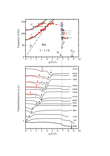
Figure 2: (Color online.) The frequency–field diagram for $\mathbf{H}\parallel\mathbf{z}$ measured at $T=1.3$ K. The ESR resonances are marked by solid symbols, empty squares correspond to phase transitions observed as anomalies on $P_{tr}(H)$ scans. The dotted line shows the transition field into the fan state. Solid lines are theoretical curves $\nu(H)$ computed for the spiral state. Dash-dotted line is the paramagnetic $\nu(H)$. Bottom panel: examples of $P_{tr}(H)$-scans measured at $T=1.3$ K.

Our main results are summarized in the frequency–field ($\nu$–$H$) diagrams, Figures 2, 3, and 5, which show the frequency dependence of resonance fields for the three principal field orientations. Two excitation branches with distinct zero field gaps are observed in each case providing clear evidence for a substantial biaxial anisotropy in the system. The field behavior of the ESR gaps allows to distinguish different magnetic structure identified for linarite in the neutron diffraction experiments, see Fig. 1. Detailed comparison with theoretical predictions is performed for the cycloidal and the conical spirals as well as for the field-induced commensurate antiferromagnetic state. In the narrow field region occupied by the fan phase, the resonance lines substantially broaden and do not allow for a meaningful comparison with the theory.

III.2.1 Magnetic field parallel to the $z$-axis

Figure 2 shows the frequency-field diagram together with examples of the field scans of transmitted through the resonator high-frequency power ($P_{tr}(H)$) measured at $T=1.3$ K for applied field oriented perpendicular to the spiral plane: $\mathbf{H}\parallel\mathbf{z}$. In this orientation, a conical or an umbrella state is realized in a wide range of fields up to the transition ($H_{F}$) into the fan phase in the close vicinity of the uniformly magnetized “saturated” phase (see bottom panel of Fig. 1). Transition to the fan phase is detected on $P_{tr}(H)$-scans as a step-like deflection. The singularity fields measured at different frequencies are shown at the frequency–field diagram with open symbols. The obtained value of $H_{F}$ is in full agreement with the values reported in Ref. Cemal_2018 .

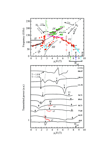
Figure 3: (Color online.) Upper panel: the frequency–field diagram for $\mathbf{H}\parallel\mathbf{y}$. Resonances corresponding to absorption lines measured at different temperatures are shown by symbols of different colors (blue squares – $T=0.5$ K, red squares – $T=1.3$ K, green rectangles – $T=1.8$ K). Empty squares are measured transition fields. The vertical dotted lines show transition fields from the bulk measurements Povarov_2016 obtained for $T=0.5$ K ($\mu_{0}H_{C}=2,7$ T, $\mu_{0}H_{F}=8$ T), $T=1.3$ K ($\mu_{0}H_{C}=2,7$ T, $\mu_{0}H_{F}=6.7$ T) and $T=1.8$ K ($\mu_{0}H_{C}=2.8$ T, $\mu_{0}H_{F}=6$ T). Solid black and purple lines show theoretical curves $\nu(H)$ computed for spiral and canted antiferromagnetic phases. Dash-dotted line is the paramagnetic line. Bottom panel: examples of $P_{tr}(H)$. Upper line was measured at $T=1.8$ K, other lines – at $T=1.3$ K.

The resonance fields measured at different frequencies are shown by solid symbols. The diagram features two ESR gaps in the spiral phase denoted as ‘I’ and ‘II’, which rise with increasing magnetic field. The error bars for some of the points illustrate characteristic values for the width at the half-height of the absorption lines. The asymptotic slope of low-frequency branch ‘I’, $\nu_{1}\to\gamma\eta H$, determined by the susceptibility anisotropy of the spin spiral is smaller than the inclination of the paramagnetic resonance $\nu/H=\gamma$ shown by the dash-dotted line. Fitting the experimental data with the theoretical formula Eq. (II.3) is shown by solid lines. The parameters obtained from these fits are $\nu_{10}=73\pm 1$ GHz, $\nu_{20}=114\pm 2$ GHz, and $\chi_{\perp}/\chi_{\parallel}=1.85\pm 0.1$. The $g$-factor values used in our computations, $g_{y}=2.1$, $g_{x}\approx g_{z}=2.3$, are taken from Wolter_2012 . The same parameters are also used for theoretical fits in other field geometries, Figs. 3–7. The value of $\chi_{\perp}/\chi_{\parallel}=1.85\pm 0.1$ agrees with the result from static magnetization measurements $\chi_{\perp}/\chi_{\parallel}=1.6\pm 0.1$ Yasui_2011 , which were performed at somewhat higher $T=2$ K and, thus, are further away from the zero temperature limit. A brief comparison of the obtained result and theoretical values derived for several sets of microscopic exchange parameters is deferred to Sec. IV.

III.2.2 Magnetic field parallel to the $y$-axis

The upper panel of Fig. 3 presents the $\nu$–$H$ diagram for $\mathbf{H}\parallel\mathbf{y}$ combining data from several temperatures: $T=0.5$ K, $T=1.3$ K, and $T=1.8$ K . For illustration we show on the lower panel examples of the power absorption scans $P_{tr}(H)$. Anomalies corresponding to the phase transitions from the spiral to the commensurate antiferromagnetic phase and from the antiferromagnetic phase to the fan phase are well detected on $P_{tr}(H)$-scans. The anomaly fields measured at different frequencies are shown by empty symbols. The transition fields exhibit significant temperature dependence. Summarizing the data observed at different frequencies and temperatures, the field ranges of transitions are marked by vertical lines. The transition from the fan to saturated phase shows no deflections on the $P_{tr}(H)$-scans. Values of the saturation field shown in the Figure are taken from Ref. Povarov_2016 .

The resonance fields obtained at different frequencies are shown on the diagram with solid squares. The error bars for selected points indicate the characteristic width at the half-height of the absorption lines. The resonance lines measured with the quasioptical technique have complicated shapes because the transmission of high-frequency (HF) power through a small diaphragm with the linarite sample of a nonregular shape depends not only on the real part of the HF-susceptibility but also on the imaginary part. Elongated shaded rectangles on the $\nu$–$H$ diagram corresponding to this frequency range mark the full area of peculiarities on $P_{tr}(H)$ scans.

In the low-field region $H<H_{C}$ linarite has the incommensurate spiral magnetic structure Willenberg_2016 . For $\mathbf{H}\parallel\mathbf{y}$ only one field-increasing branch was detected marked as ‘I’ on the diagram. This branch has the energy gap $\nu_{10}=73$ GHz. Branch ‘II’ corresponding to $\nu_{20}=114$ GHz is field independent for this orientation, which precludes its observation in the field-scan measurements. Nevertheless, this branch can be detected for the two other field directions $\mathbf{H}\parallel\mathbf{x},\mathbf{z}$.

In the field region $H_{C}<H<H_{F}$ with the canted antiferromagnetic structure the two intensive resonance absorption lines have been detected: the field increasing branch ‘IV’ and the declining branch ‘V’. We ascribe these branches to oscillations with the wave vectors $\mathbf{k}=(0,0,0)$ and $(0,0,\pi)$, specific to the commensurate two-sublattice structure. The solid red lines show the theoretical spectra Eq. (30) computed using $J_{1}=-14.5$ meV and $J_{c}=0.7$ meV, $\delta/\varepsilon=2.4$ obtained previously from the ESR gaps in zero field and adjusting the remaining parameter as $\varepsilon=0.006$. For these fits we have chosen the set of exchange parameters obtained from the INS measurements in the saturated phase Cemal_2018 , since these parameters are not affected by quantum fluctuations.

Figure 4: (Color online.) Upper panel: The temperature evolution of the power absorption scans $P_{tr}(H)$ measured at $\nu=77.72$ GHz for $\mathbf{H}\parallel\mathbf{y}$. The roman numbers correspond to the notations of branches in Figs. 1 and 3. Bottom panel: temperature dependence of the lowest zero-field gap $\Delta_{1}$.

In addition to these resonances, a narrow low-intensity absorption line (branch ‘III’) was also detected for $H>H_{C}$. Its intensity decreases with the increasing field (frequency) and vanishes at $\mu_{0}H\sim 4$ T. The additional branch can be ascribed to oscillations of spiral spin-floped structure. We suggest that the branch ‘III’ corresponds to the absorption in the part of our sample which continues to be in the spiral phase after the spin plane reorientation. Indeed, the computed value of the spin-flop transition field for $\mathbf{H}\parallel\mathbf{y}$ is equal to $\mu_{0}H_{\rm sf}^{y}=2.8~{}\pm~{}0.2$ T, see Eqs. (35) and (41), which is somewhat larger but close to the transition into the canted commensurate phase $\mu_{0}H_{C}=2.7$ T realized experimentally. Theoretical dependence $\nu(H)$ for the spiral phase above the spin-flop transition $H>H_{\rm sf}^{y}$ is shown in Fig. 3 with the dashed line. The angular dependence of the resonance field of the line ‘III’ is also satisfactorily explained by oscillations of spiral spin structure (see Fig. 7). For this reason we suppose that the transition to the canted antiferromangetic phase is broad and in the field range $2.5$ T$<\mu_{0}H<4.5$ T commensurate and spin-floped spiral phases coexist. Coexistence of the low-field incommensurate spiral and the high-field commensurate antiferromagnetic phase was also found in several previous studies and was assigned to the region II on the phase diagram of Ref. Willenberg_2016 .

The field-decreasing branch ‘V’ detected in the canted commensurate phase continues smoothly into a much broader line ‘VI’ in the high-field region. The similarity of the ESR spectra in the two phases yields further support to the presence of the fan phase near $H_{\rm sat}$ Cemal_2018 . The other suggestion for the high-field region advocated in literature is the longitudinal spin-density wave (SDW) state Willenberg_2016 ; Heinze19 . Indeed, the SDW state was found in another $J_{1}$–$J_{2}$ chain material LiCuVO₄ at intermediate fields. However, it exhibits quite different ESR spectra from what we observe in linarite Prozorova16 . Resonance frequencies measured at $T=0.5$ K (blue squares at the $\nu$–$H$ diagram) are extrapolated to zero at the saturation field $H_{\rm sat}$.

Figure 4 shows the temperature evolution of $P_{tr}(H)$-scans measured at $\mathbf{H}\parallel\mathbf{y}$, $\nu=77.72$ GHz. The $P_{tr}(H)$-scans are normalized to $1$ at $H=0$ and shifted along the ordinate axis for visibility. The shift of singularities with temperature is in good agreement with transition lines between spiral, canted commensurate, and fan phases of the $H$–$T$ diagram obtained from the bulk measurements in Povarov_2016 . The shift of the resonance line ‘I’ to higher fields with temperature can be explained by temperature decrease of the energy gap $\nu_{10}$. The bottom panel of Fig. 4 illustrates the temperature dependence of the energy gap $\nu_{10}$. The gap vanishes in a close vicinity of the transition temperature $T_{N}=2.8$ K.

III.2.3 Magnetic field parallel to the $x$-axis

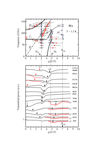
Figure 5: (Color online.) Upper panel: the frequency–field diagram for $\mathbf{H}\parallel\mathbf{x}$. The solid lines show theoretical $\nu(H)$ computed for the spiral phase before and after the spin-flop transition. Dashed lines indicate the transition fields. Dash-dotted line gives the paramagnetic $\nu(H)$. Bottom panel: examples of $P_{tr}(H)$ recorded at $T=1.3$ K.

The upper panel of Fig. 5 shows the frequency–field diagram measured at $T=1.3$ K for $\mathbf{H}\parallel\mathbf{x}$. The power transmission field scans $P_{tr}(H)$ allow to observe anomalies corresponding to the spin-flop reorientation as well as to the phase transitions between the spiral and the fan phases and between the fan phase and the saturated state. The two ESR branches, marked as ‘I’ and ‘II,’ are distinguished in the spiral phase for fields below the spin-flop transition. The lower branch ‘I’ corresponds to oscillations of the spiral plane around the $x$-axis and is expected to be independent of the applied field, see Sec. II. Nevertheless, a weak decrease of the corresponding ESR gap with magnetic field is clearly seen in the experimental data. We exclude a small field misorientation as a possible reason for that since the spin-flop transition remains quite sharp.

The discrepancy with the theory may be caused either by strong distortions of the spin structure induced by the field applied in the spiral plane or by deviations from the minimal spin model. In particular, our spin model does not include a staggered component of the $g$-tensors of copper ions and the Dzyaloshinskii-Moriya interaction on the nearest-neighbor bonds. These may be also the reason for the discrepancy between the calculated $\mu_{0}H_{\rm sf}^{x}=4$ T and the experimental $\mu_{0}H_{\rm sf}^{x}=3$ T values of the spin-flop transition field into the conical state. In the region of the fan phase a broad resonance absorption line has been observed marked as ‘IV’ in the $\nu$–$H$ diagram.

III.2.4 Magnetic field within $xz$- and $yz$-planes

Figure 6: (Color online.) Angular dependence in the $xz$ plane of the resonance field for $\nu=80.6$ GHz, solid squares, and the phase transition fields, empty symbols, measured at $T=1.3$ K. The solid line is a theoretical curve computed for the spiral magnetic structure. Dotted lines are guides for the eye.

The angular variations of the resonance field for $\nu=80.6$ GHz and the phase transition fields are presented in Figs. 6 and 7 for magnetic fields rotated in the $xz$- and the $yz$-planes, respectively. The data have been collected at $T=1.3$ K. The transition from the fan to the saturated phase is added to the figure from the $\nu$–$H$ diagram measured at $\mathbf{H}\parallel\mathbf{x}$ (Fig. 5). Transition fields $H_{sat}$ for $\mathbf{H}\parallel\mathbf{y}$ and $\mathbf{z}$ marked in the figures by diamonds, are taken from Refs. Povarov_2016 ; Cemal_2018 . The solid lines in the angular dependences show the computed dependences of resonances corresponding to branches ‘I’ and ‘III’ in spiral phase. The theoretical curves are in agreement with experimental points in low field range. At higher fields the discrepancy increases, probably due to essential distortion of the spin structure. Note here, that the additional branch ‘III’ is satisfactorily fitted by the spectrum of oscillations of the spin-floped spiral state inside the field region, where the canted antiferromagnetic state is stable. As we already remarked before, this observation fully agrees with the conclusion reached in the previous works about coexistence of commensurate and spin-floped spiral structures at fields above $H_{C}$ at $\mathbf{H}\parallel\mathbf{y}$ Willenberg_2016 ; Povarov_2016 .

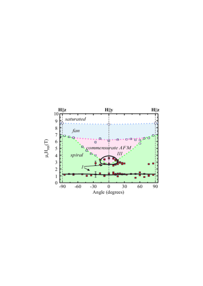
Figure 7: (Color online.) Angular dependence in the $yz$ plane of the resonance field for $\nu=80.6$ GHz, solid squares, and the phase transition fields, empty symbols, measured at $T=1.3$ K. The solid lines are theoretical curves computed for the spiral magnetic structure. Dotted lines are guides for the eye.

IV Summary and discussion

We begin by summarizing the magnetic parameters of linarite extracted from theoretical fits of the ESR spectra. The spiral magnetic structure is characterized in zero field by two susceptibilities: parallel $\chi_{\parallel}$ and perpendicular $\chi_{\perp}$ to the spiral plane with $\chi_{\perp}/\chi_{\parallel}=1.85~{}\pm~{}0.1$. This value is compared in Table I to the classical theory result (29) computed for various sets of the exchange parameters and with the dc magnetization measurements of Yasui et al. Yasui_2011 . Note, that our experiments were performed at $T=1.3$ K whereas results reported in Yasui_2011 correspond to higher $T=2$ K, which explains difference between the two values. Comparison with theoretical results clearly shows significance of interchain coupling for linarite and inadequacy of modelling its properties with the purely one-dimensional spin Hamiltonians. Apart from that, the three sets of microscopic couplings predict $\chi_{\perp}/\chi_{\parallel}$ fairly close to our value. The most precise values of the exchange constants are expected to be determined by the INS measurements in the saturated phase Cemal_2018 , see Table I. We ascribe the remaining 15–20% difference between the experimental and theoretical results for $\chi_{\perp}/\chi_{\parallel}$ to the quantum renormalization effect. Indeed, quantum fluctuations in linarite are non-negligible due to the dominant intrachain interactions and the discussed effect for $\chi_{\perp}/\chi_{\parallel}$ roughly matches the observed reduction of ordered moments in zero field Willenberg_2012 .

Based on the experimental values of zero-field ESR gaps and using $\chi_{\perp}=0.068\pm 0.004\ \mu_{B}$/Cu/T$=4900\pm 300$ J/T²/m³ Cemal_2018 we have obtained for the macroscopic anisotropy parameters of linarite as defined in Eq. (34): $D=30~{}\pm~{}2$ kJ/m³ and $E=12.6~{}\pm~{}1$ kJ/m³. The biaxial anisotropy is significant and, as a result, the spin-flop transition depends on the field orientation inside the helix plane. Furthermore, using the minimal microscopic model of the biaxial anisotropy (2) with the exchange constants of Cemal et al.  Cemal_2018 we have determined the exchange anisotropy parameters $\delta\approx 0.014$ and $\varepsilon\approx 0.006$. These values agree with the general result that symmetric anisotropic interactions constitute $(\Delta g/g)^{2}$ fraction of the isotropic exchange with $\Delta g$ being the anisotropic part of the $g$ factor of a magnetic ion Moriya60 . The obtained values for $\delta$ and $\varepsilon$ are more accurate than the previous estimates $\delta\sim 0.03$ and $\varepsilon\lesssim 0.003$ Cemal_2018 , since our results have been derived by directly measuring the small excitation gaps. The anisotropy parameters found in our study provide a reference point for future theoretical work on linarite.

Despite good overall agreement, there is one inconsistency between the ESR theory of a spiral antiferromagnet and the experimental behavior of resonance frequencies for ${\bf H}\parallel{\bf x}$, see Sec. III.2.3 and Fig. 5. The disagreement is probably due to extra anisotropic terms besides those included in Eq. (34). At the microscopic level extra terms can be generated either by the staggered DM interaction on the $J_{1}$ bonds or by staggered component of the $g$ tensors of copper ions both excluded in the minimal model (2). The latter interaction is probably more important since the disagreement between theory and experiments builds on with increasing magnetic field. This problem needs to be addressed in future studies on linarite.

Another point deserving special comment is why the semiclassical theory of incommensurate magnetic spirals works so well for linarite, though the material is obviously quasi one-dimensional, see Table I. We attribute this fact to well developed ordered moments found in the neutron diffraction experiments Willenberg_2012 . The related suppression of quantum fluctuations is a combined effect of magnetic anisotropy and interchain exchange coupling. Still, according to the published zero-field data Rule_2017 , the high-energy dynamics of linarite appears to be quite unusual. In particular, no excitations have been detected above 1.5 meV despite the fact that the magnon band computed within the harmonic spin-wave theory extends up to $\sim 20$ meV. Hence, the spin dynamics of linarite is far from being trivial and deserves additional experimental and theoretical investigation.

Regarding exotic multipolar quantum states argued to be realized in linarite Willenberg_2016 , our measurements do not allow for direct verification of their presence or absence. We refer to the recent NMR work Heinze19 , which leaves only a narrow window of fields 9.35 T$<\mu_{0}H<9.64$ T for a possible multipolar state in the ${\bf H}\parallel{\bf b}$ geometry. If continuous spin rotations about the field direction are present, a multipolar state is formed by condensate of bound complexes formed by $m$ spin flips. Since the total spin projection $S^{z}_{\rm tot}$ is a good quantum number in the saturated phase, each $m$ sector appears to be independent and the one with the highest critical field determines the equilibrium multipolar state. The multipolar states considered for linarite include quadrupolar or spin-nematic states with $m=2$, octupolar states with $m=3$ and other states up to $m=6$ Willenberg_2016 . However, the above classification of multipolar states fails if continuous symmetry is replaced with only discrete $p$-fold rotations about the external field direction. In this case one can characterize the magnon condensates by$\mod(m,p)$ only. The observed biaxial anisotropy in linarite leaves two possibilities: a multipolar state can be described either by $m=1$ and, thus, have the trivial dipolar symmetry or by $m=2$ corresponding to a nontrivial quadrupolar state. The quadrupolar state can additionally break the translation symmetry producing spontaneous dimerization Zhang17 . Whether such a state is realized in linarite in the narrow high-field region with ${\bf H}\parallel{\bf b}$ remains to be seen.

V Acknowledgements

We are grateful to K. Yu. Povarov and A. Zheludev for providing the linarite crystal used in our measurements and for helpful discussions of the results. We also thank M. Enderle and B. Fåk for useful comments on the manuscript. The work was supported in part by the Program of the Presidium of RAS 1.4 “Actual problems of low temperature physics”, by Russian Foundation for Basic Research (Grant No. 19-02-00194), by the Austrian Science Funds (Grant No. I 2816-N27), and by the ANR project Matadire. The low-temperature ESR measurements at $T=0.5$ K were supported by Russian Science Foundation Grant No. 17-02-01505.

References

- (1) A. V. Chubukov, Phys. Rev. B 44, 4693 (1991).
- (2) F. Heidrich-Meisner, A. Honecker, and T. Vekua, Phys. Rev. B 74, 020403(R) (2006).
- (3) L. Kecke, T. Momoi, and A. Furusaki, Phys. Rev. B 76, 060407(R) (2007).
- (4) T. Hikihara, L. Kecke, T. Momoi, and A. Furusaki, Phys. Rev. B 78, 144404 (2008).
- (5) J. Sudan, A. Lüscher, and A. M. Läuchli, Phys. Rev. B 80, 140402(R) (2009).
- (6) F. Heidrich-Meisner, I. P. McCulloch, and A. K. Kolezhuk, Phys. Rev. B 80, 144417 (2009).
- (7) R. Shindou and T. Momoi, Phys. Rev. B 80, 064410 (2009).
- (8) M. E. Zhitomirsky and H. Tsunetsugu, Europhys. Lett. 92, 37001 (2010).
- (9) S. Nishimoto, S.-L. Drechsler, R. Kuzian, J. Richter, and J. van den Brink, Phys. Rev. B 92, 214415 (2015).
- (10) B. J. Gibson, R. K. Kremer, A. V. Prokofiev, W. Assmus, and G. J. McIntyre, Physica B 350, e253 (2004).
- (11) M. Enderle, C. Mukherjee, B. Fåk, R. K. Kremer, J.-M. Broto, H. Rosner, S.-L. Drechsler, J. Richter, J. Malek, A. Prokofiev, W. Assmus, S. Pujol, J.-L. Raggazzoni, H. Rakoto, M. Rheinstädter, and H. M. Ronnow, Europhys. Lett. 70, 237 (2005).
- (12) M. Hase, H. Kuroe, K. Ozawa, O. Suzuki, H. Kitazawa, G. Kido, and T. Sekine, Phys. Rev. B 70, 104426 (2004).
- (13) T. Masuda, A. Zheludev, A. Bush, M. Markina, and A. Vasiliev, Phys. Rev. Lett. 92, 177201 (2004).
- (14) S.-L. Drechsler, J. Richter, A. A. Gippius, A. Vasiliev, A. A. Bush, A. S. Moskvin, J. Málek, Yu. Prots, W. Schnelle and H. Rosner, Europhys. Lett. 73, 83 (2006).
- (15) S.-L. Drechsler, O. Volkova, A. N. Vasiliev, N. Tristan, J. Richter, M. Schmitt, H. Rosner, J. Málek, R. Klingeler, A. A. Zvyagin, and B. Büchner, Phys. Rev. Lett. 98, 077202 (2007).
- (16) M. Baran, A. Jedrzejczak, H. Szymczak, V. Maltsev, G. Kamieniarz, G. Szukowski, C. Loison, A. Ormeci, S. L. Drechsler, and H. Rosner, Phys. Stat. Sol.(c) 3, 220 (2006).
- (17) Y. Yasui, Y. Yanagisawa, M. Sato, and I. Terasaki, J. Phys. Soc. Jpn. 80, 033707 (2011).
- (18) B. Willenberg, M. Schäpers, K. C. Rule, S. Süllow, M. Reehuis, H. Ryll, B. Klemke, K. Kiefer, W. Schottenhamel, B. Büchner, B. Ouladdiaf, M. Uhlarz, R. Beyer, J. Wosnitza, and A. U. B. Wolter, Phys. Rev. Lett. 108, 117202 (2012).
- (19) A. U. B. Wolter, F. Lipps, M. Schäpers, S. L. Drechsler, S. Nishimoto, R. Vogel, V. Kataev, B. Büchner, H. Rosner, M. Schmitt, M. Uhlarz, Y. Skourski, J. Wosnitza, S. Süllow, and K. C. Rule, Phys.Rev.B 85, 014407 (2012).
- (20) M. Schäpers, A. U. B. Wolter, S. L. Drechsler, S. Nishimoto, K. H. Müller, M. Abdel-Hafiez, W. Schottenhamel, B. Büchner, J. Richter, B. Ouladdiaf, M. Uhlarz, R. Beyer, Y. Skourski, J. Wosnitza, K. C. Rule, H. Ryll, B. Klemke, K. Kiefer, M. Reehuis, B. Willenberg, and S. Süllow, Phys. Rev. B 88, 184410 (2013).
- (21) B. Willenberg, M. Schäpers, A. U. B. Wolter, S. L. Drechsler, M. Reehuis, J. U. Hoffmann, B. Büchner, A. J. Studer, K. C. Rule, B. Ouladdiaf, S. Süllow, and S. Nishimoto, Phys. Rev. Lett. 116, 047202 (2016).
- (22) K. Yu. Povarov, Y. Feng, and A. Zheludev, Phys. Rev. B 94, 214409 (2016).
- (23) K. C. Rule, B. Willenberg, M. Schäpers, A. U. B. Wolter, B. Büchner, S. L. Drechsler, G. Ehlers, D. A. Tennant, R. A. Mole, J. S. Gardner, S. Süllow, and S. Nishimoto, Phys. Rev. B 95, 024430 (2017).
- (24) E. Cemal, M. Enderle, R. K. Kremer, B. Fåk, E. Ressouche, J.P. Goff, M. V. Gvozdikova, M. E. Zhitomirsky, and T. Ziman, Phys. Rev. Lett. 120, 067203 (2018).
- (25) Y. Feng, K. Yu. Povarov, and A. Zheludev, Phys. Rev. B 98, 054419 (2018).
- (26) L. Heinze, G. Bastien, B. Ryll, J.-U. Hoffmann, M. Reehuis, B. Ouladdiaf, F. Bert, E. Kermarrec, P. Mendels, S. Nishimoto, S.-L. Drechsler, U. K. Rößler, H. Rosner, B. Büchner, A. J. Studer, K. C. Rule, S. Süllow, and A. U. B. Wolter, Phys. Rev. B 99, 094436 (2019).
- (27) H. Effenberger, Mineralogy and Petrology 36, 3 (1987).
- (28) T. Nagamiya, Helical Spin Ordering, in Solid State Physics Vol. 20, edited by F. Seitz, D. Turnbull, and H. Ehrenreich (academic Press, New York, 1967), pp. 305–411.
- (29) L. E. Svistov, T. Fujita, H. Yamaguchi, S. Kimura, K. Omura, A. Prokofiev, A. I. Smirnov, Z. Honda, and M. Hagiwara, JETP Lett. 93, 21 (2011).
- (30) A. Orlova, E. L. Green, J. M. Law, D. I. Gorbunov, G. Chanda, S. Kr’́amer, M. Horvatić, R. K. Kremer, J. Wosnitza, and G. L. J. A. Rikken, Phys. Rev. Lett. 118, 247201 (2017).
- (31) J. Ren and J. Sirker, Phys. Rev. B 85, 140410(R) (2012).
- (32) B. R. Cooper, R. J. Elliott, S. J. Nettel, and H. Suhl, Phys. Rev. 127, 57 (1962).
- (33) B. R. Cooper and R. J. Elliott, Phys. Rev. 131, 1043 (1963); erratum: Phys. Rev. 153, 654 (1967).
- (34) R. J. Elliott and R. V. Lange, Phys. Rev. 152, 235 (1966).
- (35) B. R. Cooper, Magnetic Properties of Rare-Earth Metals, in Solid State Physics Vol. 21, edited by F. Seitz, D. Turnbull, and H. Ehrenreich (academic Press, New York, 1968), pp. 393–490.
- (36) M. E. Zhitomirsky and I. A. Zaliznyak, Phys. Rev. B 53, 3428 (1996).
- (37) H.-B. Chen and Y.-Q. Li, Eur. Phys. J. B 86, 376 (2013).
- (38) A. I. Milstein and O. P. Sushkov, Phys. Rev. B 91, 094417 (2015).
- (39) M. V. Gvozdikova, T. Ziman, and M. E. Zhitomirsky, Phys. Rev. B 94, 020406(R) (2016).
- (40) In the case of diagonal interchain coupling we use instead of Eq. (8).
- (41) B. I. Halperin and P. C. Hohenberg, Phys. Rev. 188, 898 (1969).
- (42) B. I. Halperin and W. M. Saslow, Phys. Rev. B 16, 2154 (1977).
- (43) A. F. Andreev and V. I. Marchenko, Sov. Phys. Usp. 130, 39 (1980).
- (44) I. Affleck, J. Phys.: Condens. Matter 1, 3047 (1989).
- (45) C. P. Slichter, Principles of Magnetic Resonance, 3rd edi-tion (Springer, Berlin, 1989).
- (46) I. A. Zaliznyak, V. I. Marchenko, S. V. Petrov, L. A. Prozorova, and A. V. Chubukov, JETP Lett. 47, 211 (1988).
- (47) S. I. Abarzhi, M. E. Zhitomirskii, O. A. Petrenko, S. V. Petrov, and L. A. Prozorova, Zh. Éksp. Teor. Fiz. 104, 3232 (1993) [JETP 77, 521 (1993)].
- (48) L. E. Svistov, L. A. Prozorova, A. M. Farutin, A. A. Gippius, K. S. Okhotnikov, A. A. Bush, K. E. Kamentsev, and É. A. Tishchenko, Zh. Éksp. Teor. Fiz. 135, 1151 (2009) [JETP 108, 1000 (2009)].
- (49) A. M. Kuzmenko, A. A. Mukhin, V. Yu. Ivanov, G. A. Komandin, A. Shuvaev, A. Pimenov, V. Dziom, L. N. Bezmaternykh, and I. A. Gudim, Phys. Rev. B 94, 174419 (2016).
- (50) L. A. Prozorova, L. E. Svistov, A. M. Vasiliev, and A. Prokofiev, Phys. Rev. B 94, 224402 (2016).
- (51) T. Moriya, Phys. Rev. 120, 91 (1960).
- (52) S.-S. Zhang, N. Kaushal, E. Dagotto, and C. D. Batista, Phys. Rev. B 96, 214408 (2017).