The EarthASAP mission concept for a Lunar orbiting cubesat

Abstract

There is a growing interest in Lunar exploration fed by the perception that the Moon can be made accessible to low-cost missions in the next decade. The on-going projects to set a communications relay in Lunar orbit and a deep space Gateway, as well as the spreading of commercial-of-the shelf (COTS) technology for small space platforms such as the cubesats contribute to this perception. Small, cubesat size satellites orbiting the Moon offer ample opportunities to study the Moon and enjoy an advantage point to monitor the Solar System and the large scale interaction between the Earth and the solar wind. In this article, we describe the technical characteristics of a 12U cubesat to be set in polar Lunar orbit for this purpose and the science behind it. The mission is named EarthASAP (Earth AS An exoPlanet) and was submitted to the Lunar Cubesats for Exploration (LUCE) call in 2016. EarthASAP was designed to monitor hydrated rock reservoirs in the Lunar poles and to study the interaction between the large Earth’s exosphere and the solar wind in preparation for future exoplanetary missions.

*Ana I. Gómez de Castro, aig@ucm.es

1 Introduction

Cubesat technology started back in 1999. At that time, the California Polytechnic State University and the Stanford University produced the basic CubeSat specifications as an attempt to facilitate the design, manufacture, and testing of small satellites. Cubesats are modular structures with unit (1U) of dimensions $10\times 10\times 10$ cm³ and weight smaller than 1.5 kg that use commercial-of-the-shelf (COTS) products. Usually, they are stacked in 2U, 3U up to 20U platforms originally intended for low Earth orbit (LEO) where the electronic components are not submitted to the hard environment of interplanetary space.

The increasing interest on Lunar exploration and the on-going initiative to build the Deep Space Gateway has open the path to the development of lunar cubesats. This new generation will need to confront important challenges such as the adaptation to interplanetary space or the development of communication strategies based on shared communications relays. Moon’s orbit offers ample opportunities to study the Moon and enjoys an advantage point to monitor the the Solar System and the large scale interaction between the Earth and the solar wind.

In recognition of this interest, the European Space Agency (ESA) focused the 2016 SysNova call on lunar cubesats (LUCE); ESA’s SysNova calls open regularly aiming at getting innovative proposals in space technology. LUCE Sysnova technical challenge was intended to address four different topics: lunar resource prospecting, environment and effects, science from or in the Moon and lunar exploration technology and operations demonstration. The first version of the project we present in this article was submitted to this call, though it was not selected it evolved and matured to address some critical challenges such as the required instrument miniaturization, the propulsion for orbit maintenance or the on-board autonomy assuming sparse communication windows to an international communication relay. The project was named Earth AS An exo-Planet (EarthASAP) as one of its key scientific objectives is using the lunar orbit vantage point to monitor the interaction between the Earth’s exosphere and magnetosphere with the solar wind; also in preparation for the coming exoplanetary research missions.

In the following sections the scientific objectives (section 2), the mission concept (section 3), the mission and data handling (section 4) are described. The article concludes with a brief summary together with the risk evaluation and the palliative solutions proposed by the team (section 5).

2 Scientific objectives

EarthASAP is intended to be in lunar polar orbit and run three research programs: the observation of the Earth’s magnetosphere and exosphere, the detection of diffuse matter within the heliosphere (comets, asteroids, and dusty clouds) and the monitoring of the water content and space weather in the lunar poles.

2.1 Earth interaction with the solar wind

There is increasing evidence of the coupling between the upper atmospheric layers (upper thermosphere) to the plasmasphere, the magnetosphere and to space weather conditions[1]. At the base of the exosphere, a population of energetic hydrogen atoms is generated as a result of this coupling. This layer is critical to understand the Earth’s thermal flow and particle escape, i.e. the planetary wind, as well as its relation with solar activity.

The most sensitive tracer to measure the distribution of exospheric hydrogen is the Lyman $\alpha$ (Ly$\alpha$) transition. Space probes such as the Imager for Magnetopause-to-Aurora Global Exploration (IMAGE[2]) or the Two Wide-angle Imaging Neutral-atom Spectrometers (TWINS[3]) mission have used Ly$\alpha$ to derive the distribution of hydrogen while navigating within the exosphere. The GEO instrument[4] on board IMAGE found that the particle density does not decrease exponentially with the distance to the Earth as predicted by the classical models[5]. In fact, the density distribution is bimodal with a dominant component peaking at 1$R_{E}$  and an extended component reaching $n_{H}=20$cm^-3 at 8$R_{E}$[6]. This result was further confirmed by the Ultraviolet Imaging Spectrograph (UVIS[7]) experiment on board the Cassini spacecraft. During Cassini’s Earth swing by, the solar Ly$\alpha$ radiation scattered by the neutral hydrogen atoms of the geocorona detected an extended exosphere around the Earth[8]. Later on, TWINS obtained the 3D distribution of Ly$\alpha$ emission within 8$R_{E}$ (and above 3$R_{E}$) around the Earth and measured even higher density values [9] (see Fig. 1). The recent images obtained by the Japanese Space Agency (JAXA) with the PROCYON probe show that the Earth’s exosphere extends further than 38$R_{E}$[10]. Extended exospheres have also been detected in Venus and Mars [11] and this seems to be a common characteristic of terrestrial planets.

Both IMAGE/GEO and TWINS reported variations in the hydrogen distribution by about $\pm 20\%$ with time that apparently are not controlled by any solar quantity or geomagnetic parameter alone [12]. A systematic monitoring of the Earth’s hydrogen envelope and escape is necessary to determine the processes controlling this evolution. The exosphere is mainly composed by neutral hydrogen that interacts very weakly with the diffuse solar wind and the Earth’s magnetic field. The exospheric ionization fraction is mainly controlled by the charge-exchange reactions between the neutral exospheric atoms and the fast charged particles accelerated by the geomagnetic field. The higher the ionization fraction, the more efficient is the solar wind in the removal of exospheric gas. A systematic long-term monitoring of the Earth’s hydrogen envelope and escape from outside of geocorona is necessary to determine the processes acting on the response of the exosphere to geostorms.

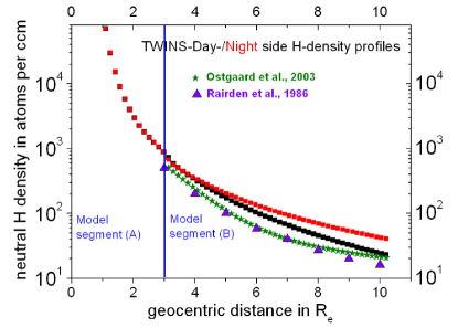
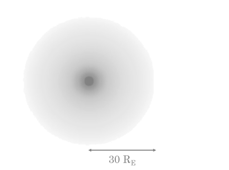
Figure 1: Left: Radial distribution of hydrogen in the Earth’s exosphere as derived from the Ly$\alpha$ measurements obtained by the TWINS mission [9]. Right: Transmissivity of the Earth (including exosphere) to background Ly$\alpha$ radiation; the radius is 30$R_{E}$[13] (black: zero transmissivity, white: full transmissivity, contrast in logarithmic scale).

Missions like IMAGE or TWINS have been orbiting the Earth within the magnetospheric cavity (the cavity size is about 70,000 km towards the Sun and extends as far as 1000$R_{E}$ towards the anti Sun, where the magnetotail is located). As a result, the interpretation of the data has been hampered by the difficulties to determine the Ly$\alpha$ emission within a complex geometry and to measure at the same time the solar flux and the heliospheric background. This issue is critical since the exospheric emission at large $R_{E}$ drops below the background Ly$\alpha$ radiation. As an example, at 10$R_{E}$ the ratio of exospheric to background Ly$\alpha$ radiation ranges between 0.21 and 1.17 depending on the strength of the variable background (estimate based on data from IMAGE [6]). The images obtained by the Lyman Alpha Imaging Camera (LAICA) on-board the PROCYON satellite show the potentials of wide field imaging from large distances to capture the faint exospheric emission above the heliospheric background.

EarthASAP is designed to map the exosphere from outside, measuring simultaneously the exospheric emission and the variable background obtaining very accurate measurements of the hydrogen distribution at large Earth radii. This is feasible at a low cost by using the Moon as a stable gravitational platform to orbit the Earth. A 3D image of the Earth’s exosphere and magnetosphere can be constructed in one synodic month.

EarthASAP’s key objective is measuring the Ly$\alpha$  source function at scales as small as 0.1$R_{E}$ (3 arcmin) and to resolve the contributions to the line excitation from solar radiation and other processes, such as collisions with high energy particles from the Sun or from internal magnetospheric sources, including the radiation belts. Moreover, EarthASAP is designed to map the exosphere/magnetosphere radiation produced by neutral oxygen (OI) and ionized helium (HeII, n=2-3 resonance transition at 164 nm). Oxygen is expected to be abundant in Earth-like planets but even for the Earth, its exospheric distribution is poorly known at large Earth radii; Oxygen is also the most highly referenced astronomical bio-signature gas. All the target tracers for the EarthASAP mission, HI, OI and HeII, are also important tracers of energetic neutral atoms (ENAs). ENAs are created in charge-exchange collisions between hot plasma ions (protons, alpha particles) and the cold neutral gas in the magnetospheric/exospheric environment. Therefore, the spatial distribution of ENAs emission indicates the location of frequent collisions with fast particles (solar wind, magnetic reconnection regions, radiation belts) and can be used as a tracer of these phenomena. The wide field imaging and the rapid read-out of EarthASAP is designed to enable monitoring variable phenomena and isolate their contribution to the total radiative budget.

2.1.1 Connection with exoplanetary research

The detection of exoplanets has opened the possibility of studying planetary exospheres and atmospheric escape in planetary systems submitted to very different stellar radiation fields and space weather conditions. The transit of planetary exospheres in front of the stellar disk produces a net absorption that has been detected in the stellar Ly$\alpha$ profile of large, massive planets in close orbit around their parent stars: HD 209458b [14], HD 189733b [15] and GJ 436b [16, 17]. The next step is measuring atmospheric escape in Earth-like exoplanets. The first evaluations are promising, especially for planets orbiting in the habitable zone around M-type stars [13]. The high optical depth of the Ly$\alpha$ line results in very low gas columns ($N_{H}>5\times 10^{17}$ cm^-2) being sufficient to block the Ly$\alpha$ radiation from the star without producing noticeable effects in the rest of the stellar spectral tracers [18]. The radius at which Ly$\alpha$ becomes optically thick, $\tau_{\text{Ly$\alpha$}}>1$, sets the geometric cross section of the planet to the Ly$\alpha$ radiation which is significantly larger than the planet itself. As a result, the transit duration and the shape of the Ly$\alpha$ light curve depend strongly on exospheric properties. Observations of exoplanetary Ly$\alpha$  transits will enable understanding the interaction of the Earth’s atmosphere with the Sun at the time when life emerged on Earth, an uncertain date between 2.7 and 4.3 Gyr ago [19]. In preparation for these activities, a better understanding of the Earth’s environment is required.

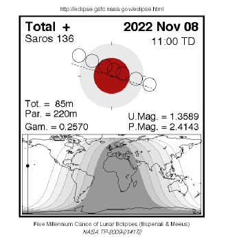
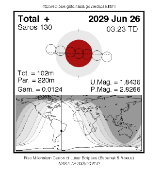
Figure 2: Earth-Moon configuration during the next total lunar eclipses: November $8^{th}$, 2022 and June 26th, 2029. At central eclipse, the Earth, the Moon and the Sun are nearly aligned enabling a unique observation of the Earth’s geocorona from Lunar orbit.

2.1.2 Earth observations during lunar total eclipses

During the next lunar eclipses of November $8^{th}$, 2022 and June 26th, 2029, there will be a unique chance to observe the Earth’s exosphere while transiting the solar disk (see Fig. 2). This viewing angle will provide exclusive information on the scattering and absorption of solar photons by the uppermost layers of the Earth’s atmosphere to compare with the theoretical predictions of the Ly$\alpha$ light curves.

2.2 Diffuse matter within the heliosphere: comets, asteroids, and dusty clouds

The resonant scattering of solar Ly$\alpha$  photons by neutral hydrogen within the heliosphere produces a bright far ultraviolet background first reported from OGO-5 data [20, 21]. The slow flow of hydrogen atoms comes from the Local Interstellar Cloud (LIC); as the Solar System crosses the LIC, the heliosphere creates a shock front that only neutral particles can penetrate. The shock front is at 94 AU from the Sun [22] in the upwind direction, ecliptic longitude (J2000) $225^{o}.4\pm 0.^{o}5$ and latitude $5^{o}.1\pm 0.^{o}2$ [23]. The heliospheric Ly$\alpha$ intensity varies as the Sun rotates, especially at low latitudes since the Sun’s ultraviolet emission is enhanced in localized active regions; however variations occur at a slow pace [24].

Surveying systematically the heliosphere in Ly$\alpha$  enables the detection and study of comets photoevaporation. Ly$\alpha$  observations are an ideal tool for searching for comets since neutral hydrogen is the main component of the coma. These observations can be used to derive the water production rate of the comet as a function of time [25, 26]. EarthASAP is designed to grow on the experience of SOHO/SWAN providing higher angular resolution ($0.05^{o}$ instead of $1^{o}$) and a wide field of view to study the detailed structure of the evaporation process and the interaction of the coma with the heliospheric magnetic field. This extra angular resolution will result in an enhanced detectability since cometary tails are clumpy structures. High resolution imaging of hydrogen distribution in the comet envelop and tail is a very sensitive probe to study comets’ photoevaporation and ionization by solar photons. Moreover, the tail interacts with the solar wind through magnetic processes and charge-exchange reactions; hence, UV observations are very useful to study the solar wind properties along the path of the comet [27]. EarthASAP angular resolution is designed to be similar to that of ALICE[28].

The far ultraviolet range is very sensitive to small dust columns. As a result, dust clouds in the Earth-Moon environment can be monitored such as those located in the libration points or those associated with small bodies streams such as the Orionids, Taurids or Leonids orbits.

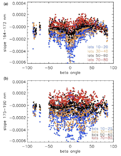
Figure 3: Measurements of lunar hydration using LAMP [29]. The slope is plotted versus beta angle: (a) 164-173 nm and (b) 175-190 nm. Negative beta angles correspond to morning, positive beta angles correspond to afternoon. Average slopes in each 10^o beta angle range are overploted as thick lines.

2.3 Water content and space weather in the Moon poles

Future lunar settlements will be most likely be sited on the Moon poles. Thus, it is crucial to determine the abundance of the water content in hydrated rocks. The instrument Lyman Alpha Mapping Project (LAMP) on board the Lunar Reconnaissance Orbiter [30] mapped the hydration and weathering of the lunar terrain by measuring the slope of the UV spectrum in 164-190 nm range [29]. The presence of a strong water absorption edge in the far-UV (near 165 nm) enables the study of lunar hydration by a simple linear fitting of the reflectance spectrum in the 164-173 nm range, where even the small water abundance affects significantly the slope. As shown in Figure 3, significant variations are detected with latitude; these variations are compared with the slope in the 175-190 nm range that it is not affected by hydration effects. In fact, the analysis of LAMP dayside data shows that the 175-190 nm region is a good indicator of weathering and composition [31]. The steeper (redder) slopes are consistent with increased hydration earlier and later in the day, and at higher latitudes.

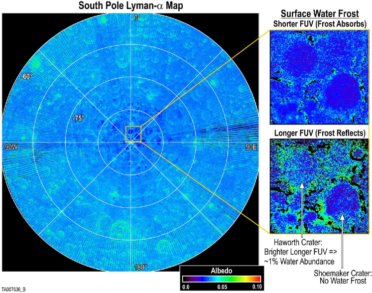
Figure 4: Measuring the hydration of rocks on the lunar south pole from FUV imaging. [Courtesy from NASA, LRO/LAMP mission.]

EarthASAP is designed to monitor the poles with a wide field of view (roughly 174km $\times$ 262km) per image and a resolution of $\sim 430$m. Though LRO/LAMP images have better resolution (down to 100m [32]) EarthASAP’s wide field of view makes feasible differential measurements of the far UV emission variability and hence, of the variations of surface ice and frost in the polar regions. In Figure 4, the procedure is illustrated from the images obtained by LRO/LAMP of the south lunar pole.

2.3.1 Clouds of dust in the Moon

During the Apollo era, astronauts saw horizon glow and streamers in the Moon’s outmost atmosphere, or ”exosphere”. Since then, many scientists have suggested that these phenomena were caused by sunlight scattered by dust grains in the exosphere. Questions about how lunar dust and dusty plasmas are charged, mobilized and transported remain at the centre of dusty plasma studies. EarthASAP is designed to answer these questions by detecting the presence of dust clouds and plumes, as well as their interaction with solar radiation and particles.

3 Mission concept

The EarthASAP mission covers several science themes devoted to the study of the Earth and the Moon, listed in Table 1. The previous section presented the desired science goals, that are achieved by different objectives, which in turn, impose the mission requirements. In Table 1 also the specific results to be obtained are shown.

Table 1: Scientific goals, requirements and results traceability matrix

Theme	Earth interaction with Solar Wind
Goal	To observe the Earth’s magnetosphere and exosphere in UV
Specific Objectives	Requirements	Results
• Imaging capabilities in FUV range from $115$nm to $180$nm. • To fit the Earth’s magnetosphere in one single image • To resolve structures in the Earth’s exosphere $<0.1$$R_{E}$ • To observe the spatial distribution of ENAs	• Solar blind detection system in the $115$nm to $180$nm range • Field of view $22^{o}\times 20^{o}$ • Angular resolution better than $3$ arcmin • FUV range, includes Ly$\alpha$(121.6nm), OI ($130.3$nm) and HeII ($164.0$nm). Narrow band filtering (FWHM=$5$nm) at these wavelengths is needed	• Production of first $3$D map of Earth’s exosphere • Determination of the exospheric emission and transfer function of Ly$\alpha$ photons through the Earth’s exosphere.
Theme	Diffuse matter within the heliosphere
Goal	To detect extended features against the heliospheric UV background
Specific Objectives	Requirements	Results
• Detect the $0.16$kR exospheric Ly$\alpha$ emission at 15 $R_{E}$ over the heliospheric background with SNR=$10$ • To resolve structures in the Earth’s exosphere $<0.1$$R_{E}$	• (FoV and angular resolution as above)	• Derivation of the water production rate of a comet as function of time • Produce maps with new extended features such as comet tails, dust clouds and HI filaments • Planet $9$ might be detected if surrounded by a cloud of small bodies and dust from outer Solar System

Table 2: (Cont.) Scientific goals, requirements and results traceability matrix

Theme	Water content on the Moon poles
Goal	To image lunar hydration, including FUV variability
Specific Objectives	Requirements	Results
• Image the lunar poles • Imaging spots of around $175$ km $\times$ $260$ km • Resolve structures on the lunar surface $<0.5$ km size • Differential measurements, analysis of FUV slope	• Lunar polar orbit • (FoV and angular resolution as above) • Narrow band filtering at $170$nm, $175$nm, $187$nm and $190$nm	• Time series of water contents on the Moon’s poles
Theme	Space weather on the Moon poles and lunar exosphere
Goal	To detect the presence of dust clouds and plumes in the lunar exosphere
Specific Objectives	Requirements	Results
• Detect and qualify dust clouds • Detect the 0.16kR exospheric Ly$\alpha$ emission at 15 $R_{E}$ over the heliospheric background with SNR=$10$	• (FoV and angular resolution as above) • Step filter (f.i,, F2Ba) to be used together with no-filter to measure extinction • Efficiency of the optical system and aperture	• Confirm if sunlight scattered by dust grains produce the observed features such as horizon glows and streamers

These scientific requirements can be fulfilled by the EarthASAP proposal, based on 12U cubesat, with 8U dedicated to the scientific payload and 4U to the service module.

3.1 Scientific payload

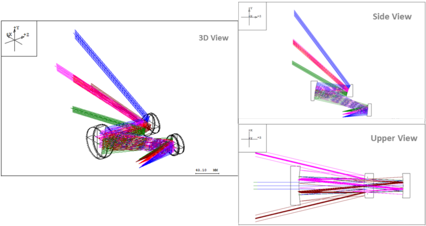
Figure 5: Optical layout for the WALRUS system implementation.

The optical design of the imager is an evolution of the Wide Angle Large Reflective Unobscured System (WALRUS [33, 34]). It is a three-element mirror system, with spherical primary and tertiary mirrors and a prolate secondary that results in a system completely free of chromatic aberrations, with a wide field of view ($22^{o}\times 20^{o}$), focal-ratio of $f/4.5$ and a compact design ($65\times 115\times 190$mm³) suitable for a cubesat. It also provides an excellent image quality with flat field, covering the spectral range 100-300 nm. The optical layout is presented in Fig. 5 and the parameters of the proposed designed are listed in Table 3. Filters will be inserted in a filter wheel before the detector; based on previous developments [35, 36, 37] a transmittance of 7% with high out-of-band rejection is expected in the narrow band line filters tuned to Ly$\alpha$, OI and HeII.

The payload module is assumed to weight 8 kg, consume 4W and require a pointing accuracy of $14^{\prime\prime}$ ($3\sigma$). Due to the dimensions of the telescope, the payload module requires a 8U system including the detector, an MCP with CMOS read-out. The focal length and image size of the telescope are compatible with the use of the multichannel plate PHOTEK image intensifier MCP118, with an input window of MgF₂, a photo-cathode of CsI and a phosphor anode of P46/P47. The MCP118 image intensifier has a typical effective resolution of 40-50 lp/mm, leading to an effective sampling size of around 15$\mu$m and resulting in 2.5 samples inside the optics blur diameter of 0.04mm. We have checked that it is actually possible to reduce that blur diameter for all points in the field of view to get 500 effective samples across the detector size of 18mm. The CMOS detector is planned to be an AMS (CMOSIS) 5.5$\mu$m pixel size based on previous experience.

The encircled energy of the proposed design is included in Figure 6. As shown, the preliminary optimization performed is enough to bring the optics blur diameter to a value lower than 0.04mm, for all points in the field of view. This will result in the optics providing around 500 effective samples across the detector size of 18mm. The proposed optical design is subjected to a moderate amount of barrel distortion (peak value of -4.5%), as can be observed in Figure 7. This effect will be corrected for as part of the image post-processing and thus it is not considered relevant in terms of overall optical performance. The simulated effect of both the image quality and optical distortion of the proposed design on the Earth’s image is also displayed in the figure.

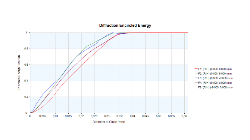
Figure 6: Encircled energy of the proposed design.

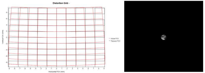
Figure 7: Left: Optical distortion of the proposed design. Right: Simulation of the Earth image as seen with the proposed design

Sensitivity requirements are met with this design and configuration. The Ly$\alpha$  emission from the Earth’s exosphere can be mapped with SNR$>$10 up to 15$R_{E}$  from the Earth’s centre. Under the worst conditions (solar zenital angle $90^{o}$), the exosphere produces a Ly$\alpha$  flux of 0.16kR at 15$R_{E}$  that is observed agains a 1.1kR heliospheric background [38, 39]. At the Moon’s distance, the count rate from 15$R_{E}$  is expected to be 115 counts s^-1 per angular resolution element ($0.05^{o}$ or 335km²) at the telescope entry pupil. However, UV optics is not very efficient; the expected transmittance of the optical system at Ly$\alpha$  is about 2% and the detector QE at this wavelength is  30%. As a result, the count rate per angular resolution element on the detector is significantly lower (0.69 counts s^-1) and it will be spread in $\sim$6 pixels to sample the PSF by $2.5\times 2.5$ pix²; SNR = 10 will be reached in less than 15 minutes with the optical elements and MCP detectors proposed for EarthASAP. The measurements will be made in TIME-TAG mode with the detector being read every 40ms, therefore the total count rate will be 280,000, well within the safety margins of conventional MCP detectors. These calculations are made using state of the art technology; the baseline MCP detector is currently under development for the WSO-UV mission [40] and it is based on the heritage of the ISSIS instrument [41] though its QE has been enhanced to reach the sensitivity of the Hamamatsu detectors used in the Lyman Alpha Imaging Camera (LAICA) on board the Japanese micro-spacecraft PROCYON with a rather similar optical configuration [42]. Similar results have also been obtained by SOHO/SWAN [43].

3.2 Service module

Table 3: Telescope parameters for the adapted WALRUS system. The stated dimensions correspond only to the presented optical layout, prior to baffling for stray-light control.

Parameter	Value
Type	All-reflective (WALRUS)
Focal Length	48 mm
F-number	$f/4.5$
Spectral range	100-300nm
Image Size	18mm
Field of View	($22^{o}\times 20^{o}$)
Encircled energy diameter	$<0.05^{o}$
Dimensions $(X\times Y\times Z)$	$65\times 115\times 190$mm3

The service module has been sketched selecting some COTS cubesats components listed in Table 4, that will be implemented within 4 additional units. Therefore, the complete configuration will be a 12U cubesat, $3\times 2\times 2$. All these elements, service module and payload can be integrated in the $12$U cubesat as seen in Fig. 8.

Table 4: Service module components for EarthASAP.

Unit name	Model and Supplier	Mass	Power	Volume
		(g)	consumption	(mm3)
Solar panel	P110A GOMSpace (DK)	29	2300mW	$98\times 91.6\times 5.5$
Star Tracker	St-400 Hyperion Technologies (NL)	280	700mW steady	$53.8\times 53.8\times 90.5$
Reaction wheels	RW400 Hyperion Technologies (NL)	340	$<2500$mW peak	$50\times 50\times 27.5$
Reaction Control system	GOMSpace (DK)	220	$2$W peak, $0.35$W standby	$100\times 100\times 30$
On board computer	CP400.85 Hyperion Technologies (NL)	7	$<1000mW$ peak	$20\times 50\times$ 10
Telemetry Unit	S band Transmitter	85	$13$W transmitter	$99\times 93\times 15$
	ISIS High Data Rate S-Band Transmitter (NL)
Battery	NanoPowerBPX GOMSpace (DK)	500		$91.6\times 85.9\times 40$

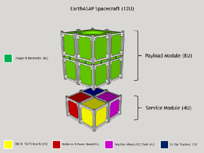
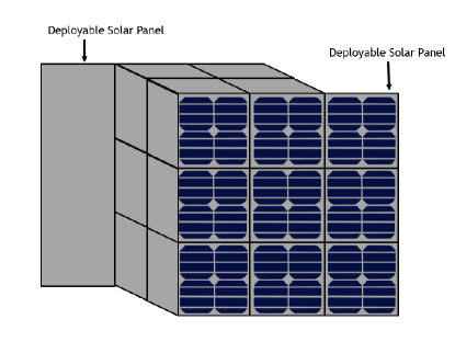
Figure 8: Integration of the proposed elements of the EarthASAP mission in a $12$U cubesat structure.

4 Observation strategy and data analysis

EarthASAP will map the Earth, its exosphere and magnetosphere, the heliosphere, and the lunar poles with a $20^{o}\times 30^{o}$ field imager and an angular resolution of $3^{\prime}$.

The satellite is designed for a low eccentricity lunar polar orbit, at 500km of the surface. EarthASAP is designed to communicate with Earth via a Lunar Orbiter in $800$ km polar orbit. Simulating the EarthASAP and the data relay orbiter a daily coverage between 13.5 and 14.5 hours is obtained. Figure 9 depicts the EarthASAP data relay Lunar Orbiter visibility.

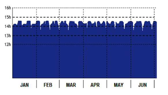
Figure 9: Estimated EarthASAP data relay Lunar Orbiter Visibility.

The orbital period is 2.64 hours. For each orbital period, a basic cycle will be implemented consisting in surveying during 64 minutes the Earth’s exosphere, 12 minutes the South pole of the Moon, 64 minutes the heliosphere and finally 12 minutes the North lunar pole. This duty cycle is sketched in Figure 10.

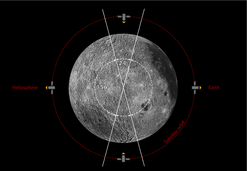
Figure 10: Mission planning for EarthASAP. While orbiting the Moon, the satellite will map systematically the Earth’s exosphere, the heliosphere and the lunar poles with an optimized duty cycle.

As the Orbiter is assumed to provide data relay services, only the fuel to correct the orbit of the cubesat is required. The communications with the Lunar Orbiter depends on the position in the orbit, but our simulations show that we could obtain a daily coverage between 13.5h and 14.5h.

The EarthASAP 500 km circular polar orbit will experiment every year two eclipse seasons. Each eclipse season will last about 3.5 months. The maximum eclipse duration will be about 45 minutes. Statistically, EarthASAP will spend 13.1% of the time in shadow. The mean eclipse duration is 36.6 minutes with a standard deviation of 9.3 minutes. In Figure 11 the EarthASAP yearly eclipse evolution with the daily hours of shadows is depicted.

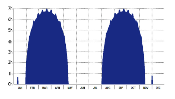
Figure 11: EarthASAP yearly eclipse evolution.

EarthASAP will produce images at a rate of 1 frame per minute in different filters. This means around $\bf{6048}$ Mbytes/day. An on board processing with a compression factor $\bf{2}$ implies total amount of TM of roughly $\bf{3629}$ Mbytes/day. This must be downloaded during the averaged $\bf{14}$ hrs when the relay spacecraft is visible, following Fig. 9. Presuming a protocol overhead of $\bf{20}$%, the required bandwidth is around $\bf{72}$ Kbytes/sec. This requirement can be fulfilled using the S-band transmitter listed in Table 4. This proposed S-band transmitter provides $\bf{537.5}$ Kbytes/sec for downlink, which is enough for our purposes.

When defining the duty plan, one must take into account the available power budget, which will determine the activation of the different elements of the spacecraft. For instance, we must consider the power consumption of the selected S-band transmitter, or the eclipse seasons. An initial power budget of the service module components and payload is found in Table 5, with a nominal consumption close to $\bf{15}$W, and a peak consumption of $\bf{21}$W.

Table 5: EarthASAP power budget.

Unit	Peak (W)	Duty Cycle (%)	Average (W)
Solar Panels (x9)	$20.7$	$70$%	$14.49$
Star tracker	$-0.7$	$100$%	$-0.7$
Reaction Wheels	$-2.5$	$25$%	$-0.6$
Reaction Control System	$-2.0$	(when needed)	$-0.35$
On board Computer	$-1.0$	$100$%	$-1.0$
TM/TC unit	$-13.0$	$58$%	$-7.6$
Payload	$-4.0$	$100$%	$-4.0$

The Reaction Control system (RCS) is needed for unloading the reaction wheels. Periodic maintenance periods will be included in the duty plan to include these activities, when the power consumption may increase. Other periods that can reduce the continuous observations are the eclipses. The batteries can provide just around $\bf{5.5}$hrs of full operations. Therefore, during eclipses, if the payload is kept is active, one may decide to interrupt the downlink of data.

During other periods, no image production will be possible. These periods are, for instance, those when the Sun constraint could be violated because the Sun enters in the FoV of the instrument when observing the Earth. This roughly happen during full moon phases, when no image acquisition is possible. The duty plan can insert maintenance activities here.

4.1 Data analysis and interpretation

The contamination by cosmic rays will be removed and geometrical distortions will be corrected on board. The optical system is designed to introduce a well-known distortion that will be evaluated on ground tests and re-assessed during commissioning. Flat fielding and an additional geometric correction to compensate for the variation of the viewing angle will also be applied on board. Note that the angular velocity of EarthASAP will be $\omega=2.3^{o}$ min^-1, resulting in a variation of the Earth projected size by a factor $\cos\omega t$, that will run faster close to the poles. A final list with event centroids and time will be generated and transferred to Earth for every pointing and filter during a given orbit.

Ground based processing will include fitting and subtraction of the heliospheric background. Lunar observations and comparison with previous missions (mainly LRO) will be used for flat fielding and calibration. Scattered solar radiation will be the main source for absolute flux calibration.

EarthASAP will take advantage of the wide field imaging to simultaneously obtain information on solar flux reaching the Earth, the ultraviolet background, and the targets (Earth, Moon, Solar System) for most objects. Protocols will be implemented to detect and track transient events such as solar flares reaching the Earth, solar storms and geo-storms.

Finally, Ly$\alpha$  maps will be used to build a 3D structure of the exosphere and determine the transfer of Ly$\alpha$  photons through it. The Ly$\alpha$  source function will be calculated directly from the data and made available to the community for future exo-Earth transit calculations and data interpretation.

5 Summary

This article summarizes the basic scientific and technological characteristics of a 12U cubesat to be set in Lunar orbit. It is shown that the small 8U payload is enough to address important problems concerning the nature of gas escape from the Earth’s atmosphere (and Earth-like planets). The small EarthASAP mission is also well suited to monitor the hydration of the rocks in the lunar poles, and the heliosphere. The observatory can be manufactured in few years, at a cost below five million euros.

Up to now, three technical problems have been identified but all can be addressed with the existing technology. First, the proposed optical design is subjected to a moderate amount of barrel distortion. However, this effect can be corrected by the post-processing of the images. Second, the proposed off-axis telescope requires a lateral input window and a deployable baffle. These two elements might be placed in the side of the payload unit but require designing a structure that allows the window to maintain the structural properties of the system. Also, a baffle or lid would be needed to close the input windows during launch and transit phases. Third, in order to align correctly the off-axis mirror system and maintain it independently of temperature changes, it is fundamental to use materials with small thermal expansion coefficient such as carbon fibre based composites or inbar.

Most important, to make the Moon accessible to EarthASAP and, in general, to lunar cubesat missions, it is required that a communications relay is set close to the Moon. This is the only means to keep their power needs within the cubesat scale.

- [1] J. Qin and L. Waldrop, “Non-thermal hydrogen atoms in the terrestrial upper thermosphere,” Nature Communications 7, 13655 (2016).
- [2] S. A. Fuselier, J. L. Burch, W. S. Lewis, et al., “Overview of the IMAGE science objectives and mission phases,” Space Science Reviews 91, 51 (2000).
- [3] D. McComas, F. Allegrini, J. Baldonado, et al., “The Two Wide-angle Imaging Neutral-atom Spectrometers (TWINS) NASA Mission-of-Opportunity,” SSRv 142, 157 (2009).
- [4] S. Mende, H. Heetderks, H. Frey, et al., “Far ultraviolet imaging from the IMAGE spacecraft. 3. Spectral imaging of Lyman-a and OI 135.6 nm,” SSRv 91, 287 (2000).
- [5] J. Chamberlain, “Planetary coronae and atmospheric evaporation,” P&SS 11, 901 (1963).
- [6] N. Østgaard, S. Mende, H. Frey, et al., “Far ultraviolet imaging from the IMAGE spacecraft. 3. Spectral imaging of Lyman-a and OI 135.6 nm,” JGRA 108, 1300 (2003).
- [7] L. Esposito, C. Barth, J. Colwell, et al., “The Cassini ultraviolet imaging spectrograph investigation,” SSRv 115, 299 (2004).
- [8] S. Werner, H. Keller, A. Korth, et al., “UVIS/HDAC Lyman-a observations of the geocorona during Cassini’s Earth swingby compared to model predictions,” AdSpR 34, 1647 (2004).
- [9] J. Zoennchen, J. Bailey, U. Nass, et al., “The TWINS exospheric neutral H-density distribution under solar minimum conditions,” AnGeo 29, 2211 (2011).
- [10] S. Kameda, S. Ikezawa, M. Sato, et al., “Ecliptic north-south symmetry of hydrogen geocorona,” Geophysical Research Letters 44, 11706 (2017).
- [11] B. D. Shizgal and G. G. Arkos, “Nonthermal escape of the atmospheres of Venus, Earth, and Mars,” Reviews of Geophysics 34, 483 (1996).
- [12] J. J. Bailey and M. Gruntman, “Investigation of Exosphere Variations by Lyman-alpha Detectors on the TWINS Mission,” in AGU Fall Meeting Abstracts, 2013, SA51A–2030 (2013).
- [13] A. I. Gomez Castro, L. Beitia-Antero, and S. Ustamujic, “On the feasibility of studying the exospheres of Earth-like exoplanets by Lyman- monitoring. Detectability constraints for nearby M stars,” Experimental Astronomy 45, 147–163 (2018).
- [14] A. Vidal-Madjar, A. Lecavelier des Etangs, J.-M. Désert, et al., “An extended upper atmosphere around the extrasolar planet HD209458b,” Natur 422, 143 (2003).
- [15] A. Lecavelier Des Etangs, D. Ehrenreich, A. Vidal-Madjar, et al., “Evaporation of the planet HD 189733b observed in HI Lyman-,” Astronomy and Astrophysics 514, 72 (2010).
- [16] J. R. Kulow, K. France, J. Linsky, et al., “Ly Transit Spectroscopy and the Neutral Hydrogen Tail of the Hot Neptune GJ 436b,” ApJ 786, 132 (2014).
- [17] D. Ehrenreich, G. Tinetti, A. Lecavelier Des Etangs, et al., “The transmission spectrum of Earth-size transiting planets,” A&A 448, 379 (2006).
- [18] A. I. Gómez de Castro, R. Loyd, K. France, et al., “Protoplanetary Disk Shadowing by Gas Infalling onto the Young Star AK Sco,” ApJ 818, L17 (2016).
- [19] R. Buick, “The earliest records of life on Earth,” in Planets and Life, W. T. Sullivan and J. A. Baross., Eds., Cambridge University Press, 237–264 (2007).
- [20] J. Bertaux and J. Blamont, “Evidence for a Source of an Extraterrestrial Hydrogen Lyman-alpha Emission,” A&A 11, 200 (1971).
- [21] G. Thomas and R. Krassa, “OGO 5 Measurements of the Lyman Alpha Sky Background,” A&A 11, 218 (1971).
- [22] E. Stone, A. Cummings, F. McDonald, et al., “Appearance of a Third Episode of Enhanced Particle Intensities at 94 AU: Voyager 1 in the Heliosheath,” ICRC 2, 43 (2005).
- [23] M. Witte, M. Banaszkiewicz, and H. Rosenbauer, “Recent results on the parameters of the interstellar helium from the ULYSSES/GAS experiment,” SSRv 78, 289 (1996).
- [24] R. Rairden, L. Frank, and J. Craven, “Geocoronal imaging with Dynamics Explorer,” JGR 91, 13613 (1986).
- [25] J. Bertaux, J. Costa, E. Qémerais, et al., “Lyman-alpha observations of comet Hyakutake with SWAN on SOHO,” P&SS 46, 555 (1998).
- [26] J. Mäkinen, J.-L. Bertaux, H. Laakso, et al., “Discovery of a comet by its Lyman-a emission,” Natur 405, 321 (2000).
- [27] B. Shustov, M. Sachkov, A. I. Gómez de Castro, et al., “Comets in UV,” Ap&SS 363, 64 (2018).
- [28] S. A. Stern, D. C. Slater, J. Scherrer, et al., “Alice: The Rosetta Ultraviolet Imaging Spectrograph,” SSRv 128, 507–527 (2007).
- [29] A. R. Hendrix, K. D. Retherford, G. Randall Gladstone, et al., “The lunar far-UV albedo: Indicator of hydration and weathering,” Journal of Geophysical Research (Planets) 117, E12001 (2012).
- [30] G. Gladstone, K. Retherford, A. Egan, et al., “Far-ultraviolet reflectance properties of the moon’s permanently shadowed regions,” JGRE 117, E00H04 (2012).
- [31] A. R. Hendrix, T. K. Greathouse, K. D. Retherford, et al., “Lunar swirls: Far-UV characteristics,” icarus 273, 68–74 (2016).
- [32] G. Chin, S. Brylow, M. Foote, et al., “Lunar Reconnaissance Orbiter Overview: The Instrument Suite and Mission,” SSRv 129, 391 (2007).
- [33] K. Hallam, B. Howell, and M. Wilson, “Wide-angle flat field telescope, us patent 4,598,981,” (1986).
- [34] K. Hallam, B. Howell, and M. Wilson, “An all-reflective wide-angle flat-field telescope for space,” in Intrumentation in Astronomy V, A. Boksenberg and D. Crawford, Eds., Proc. SPIE 445, 295–300 (1984).
- [35] L. Rodríguez-de Marcos, J. A. Aznárez, J. A. Méndez, et al., “Advances in far-ultraviolet reflective and transmissive coatings for space applications,” in SPIE, Society of Photo-Optical Instrumentation Engineers (SPIE) Conference Series 9912, 99122E (2016).
- [36] A. I. Gómez de Castro, J. Maíz Apellániz, P. Rodriguez, et al., “The imaging and slitless spectroscopy instrument for surveys (ISSIS) for the world space observatory-ultraviolet (WSO-UV),” Ap&SS 335, 283–289 (2011).
- [37] M. Fernández-Perea, M. Vidal-Dasilva, J. I. Larruquert, et al., “Novel narrow filters for imaging in the 50-150 nm VUV range,” Ap&SS 320, 243–246 (2009).
- [38] W. Pryor, S. Lasica, A. Stewart, et al., “Interplanetary Lyman a observations from Pioneer Venus over a solar cycle from 1978 to 1992,” JGR 103, 26833 (1998).
- [39] E. Qémerais, B. McClintock, G. Holsclaw, et al., “Hydrogen atoms in the inner heliosphere: SWAN-SOHO and MASCS-MESSENGER observations,” JGRA 119, 8017 (2014).
- [40] B. Shustov, A. I. Gómez de Castro, M. Sachkov, et al., “The World Space Observatory Ultraviolet (WSO-UV), as a bridge to future UV astronomy,” Ap&SS 363, 62 (2018).
- [41] A. I. Gómez de Castro, G. Belén Perea, N. Sánchez, et al., “The Imaging and Slitless Spectroscopy Instrument for Surveys (ISSIS): expected radiometric performance, operation modes and data handling,” Ap&SS 354, 177–185 (2014).
- [42] S. Kameda, M. Kuwabara, and N. Osada, “Hydrogen Lyman Alpha Imaging Camera onboard PROCYON,” in AGU Fall Meeting Abstracts, 2018, P24C–04 (2018).
- [43] I. I. Baliukin, J. L. Bertaux, E. Quémerais, et al., “SWAN/SOHO Lyman- Mapping: The Hydrogen Geocorona Extends Well Beyond the Moon,” Journal of Geophysical Research (Space Physics) 124, 861–885 (2019).