Velocity Dispersions of Brightest Cluster Galaxies and Their Host Clusters

Abstract

We explore connections between brightest cluster galaxies (BCGs) and their host clusters. We first construct a HeCS-omnibus cluster sample including 227 galaxy clusters within $0.02<z<0.30$; the total number of spectroscopic members from MMT/Hectospec and SDSS observations is 52325. Taking advantage of the large spectroscopic sample, we compute physical properties of the clusters including the dynamical mass and cluster velocity dispersion ($\sigma_{cl}$). We also measure the central stellar velocity dispersion of the BCGs ($\sigma_{*,BCG}s$) to examine the relation between BCG velocity dispersion and cluster velocity dispersion for the first time. The observed relation between BCG velocity dispersion and the cluster velocity dispersion is remarkably tight. Interestingly, the $\sigma_{*,BCG}/\sigma_{cl}$ ratio decreases as a function of $\sigma_{cl}$ unlike the prediction from the numerical simulation of Dolag et al. (2010). The trend in $\sigma_{*,BCG}/\sigma_{cl}$ suggests that the BCG formation is more efficient in lower mass halos.

1. INTRODUCTION

Brightest cluster galaxies (BCGs) are a distinctive population of luminous galaxies located in the central regions of galaxy clusters (and groups). Identification of the BCGs has a long history since 1784. Charles Messier identified a concentration of nebulæ in the Virgo constellation and found its brightest component, M87 (Biviano, 2000). Many studies used BCGs as a tracer for the systematic identification of galaxy clusters in photometric data (e.g. Abell, 1958; Abell et al., 1989; Koester et al., 2007; Hao et al., 2010).

BCGs are also a unique population that connects galaxy evolution and structure formation models. Standard structure formation models predict the hierarchical growth of massive halos of clusters through the stochastic accretion of less massive halos (van den Bosch, 2002; McBride et al., 2009; Zhao et al., 2009; Fakhouri et al., 2010; Gao et al., 2012; Kravtsov, & Borgani, 2012; Haines et al., 2018). During the mass assembly of the halos, the BCG residing in the bottom of the cluster potential may experience more mergers and thus the evolutionary path of the BCGs differs from the path for less massive galaxies (e.g. (De Lucia & Blaizot, 2007)). Detailed investigation of BCG properties and the related evolutionary processes probe cluster formation models.

The ratio between stellar mass of a BCG and its halo mass constraints both structure formation and galaxy evolution models (Wang et al., 2006; Moster et al., 2010; Leauthaud et al., 2012; Kravtsov et al., 2018). Abundance matching techniques show that this ratio has a peak at $M_{halo}\sim 10^{12}M_{\odot}$ and decreases at higher and lower halo mass (e.g. (Conroy et al., 2006; Behroozi et al., 2010; Moster et al., 2010; Guo et al., 2010)). The decline of the stellar mass fraction at high halo mass suggests that strong feedback processes (including AGN feedback) suppress the stellar mass growth of the BCGs (Silk, & Rees, 1998; McNamara & Nulsen, 2007; Kravtsov, & Borgani, 2012).

Despite the importance of BCGs, the study of BCGs is not straightforward. First of all, the identification of the BCGs is not trivial. The Coma cluster is a striking example. Coma has two bright galaxies (NGC 4874 and NGC 4889) with a small magnitude difference. Neither of these galaxies is located on the dynamical center of the cluster (Rines et al., 2016). In many cases, an apparently brightest galaxy near the cluster canter has significantly large velocity offset with respect to the mean redshift of cluster members ($>300~{}\rm km~{}s^{-1}$, Coziol et al., 2009; Lauer et al., 2014; Sohn et al., 2019) suggesting that these objects may not reside at the bottom of the cluster potential well. To avoid confusion, BCG identification requires multi-dimensional data for the galaxies in the cluster field including spatial and radial velocity distribution of the cluster members.

Measuring the physical properties of the BCGs is also not straightforward. BCGs usually have very extended stellar halo (cD galaxies, Morgan, 1958; Matthews et al., 1964) and their profiles overlap the intracluster light. Additionally, the BCGs are surrounded by many satellites galaxies. The extended stellar halo and contamination from surrounding galaxies affects BCG photometry (Gonzalez et al., 2007; Lauer et al., 2014) Bernardi et al. (2013) demonstrate that the photometry of the bright galaxies from the Sloan Digital Sky Survey (SDSS) is systematically offset from the total magnitudes estimated from more complex two-dimensional parametric fitting models. As Bernardi et al. (2013) emphasize, the systematic uncertainty in photometry propagates to the stellar mass and ultimately to the stellar mass to halo mass relation.

Here, we examine the properties of BCGs and their relation with the host cluster properties based on a large spectroscopic sample of galaxy clusters. The large spectroscopic sample enables identification of BCGs based on large sets of spectroscopically identified cluster members in multi-dimensional space. The central stellar velocity dispersion of the BCG itself is insensitive to the galaxy photometry (Wake et al., 2012; Zahid et al., 2016, 2018). We investigate the relationship between stellar velocity dispersion of the BCG and the global cluster velocity dispersion. We demonstrate that this relation provides an interesting constraint on structure formation models.

We describe the cluster and galaxy samples in Section 2. In Section 3, we introduce the HeCS-omnibus cluster catalog, a large compilation of galaxy clusters with substantial spectroscopic data. We also describe the identification of spectroscopic members and the brightest cluster galaxies. The HeCS-omnibus cluster catalog includes 227 clusters and the typical number of spectroscopic members per cluster is $\sim 180$. We explore the connection between the physical properties of BCGs and those of their host clusters in Section 4. We compare the observed properties of BCGs and their clusters in Section 5. We conclude in Section 6. We assume the standard $\Lambda$CDM model with $H_{0}=70~{}\rm km~{}s^{-1}~{}Mpc^{-1}$, $\Omega_{m}=0.3$, $\Omega_{\Lambda}=0.7$, and $\Omega_{k}=0.0$ throughout.

2. SAMPLE

2.1. Cluster Sample

Our goal is to explore the relation between the physical properties of galaxy clusters and the properties of their brightest cluster galaxies (BCGs). Spectroscopic surveys yield robust membership identification critical to BCG identification. The set of spectroscopically identified members provides physical properties of the galaxy clusters including galaxy velocity dispersion and a basis for deriving the cluster halo mass.

We built a sample of galaxy clusters with substantial spectroscopic data to examine the relation between the BCG and cluster properties. We first collected data from various spectroscopic surveys. The Cluster Infall Region Surveys (CIRS, Rines & Diaferio, 2006) includes 74 nearby clusters with redshift $z<0.10$. Rines & Diaferio (2006) collected spectroscopic data from the Sloan Digital Sky Survey (SDSS) Data Release 4 (DR4) and investigated the infall patterns of these clusters. We include 71 CIRS clusters with $0.02<z<0.10$ in our catalog and compile additional spectroscopic data including SDSS DR14 (see Section 2.2).

The Hectospec Cluster Survey (HeCS, Rines et al., 2013, 2016, 2018, in preparation) is a large spectroscopic survey of galaxy clusters using the 300 fiber Hectospec mounted on 6.5m Multi-Mirror Telescope (MMT, Fabricant et al., 2005). The first HeCS catalog (Rines et al., 2013) lists 58 X-ray flux selected clusters with $0.1<z<0.3$. HeCS-SZ (Rines et al., 2016) extends the sample by including 123 clusters selected based on Sunyaev-Zel’dovich measurements. After removing overlaps with CIRS and HeCS, there are 50 unique clusters added from the HeCS-SZ catalog. HeCS-red (Rines et al., 2018) includes another 27 high-richness ($\lambda>64$) redMaPPer clusters with $0.08<z<0.29$; we added 23 unique HeCS-red clusters to our sample. HeCS-faint is a Hectospec survey of 16 clusters with low X-ray luminosity ($L_{X}<5\times 10^{43}$ erg s^-1, Rines et al., in preparation). We exclude 4 HeCS-faint systems not covered by SDSS DR14. We include the remaining 12 HeCS-faint systems with $0.04<z<0.17$. For these HeCS clusters, we compile SDSS DR14 spectroscopy and extensive Hectospec survey data for fainter objects. The entire resulting sample includes $\sim 400-550$ redshifts per clusters.

We also include clusters from ACReS (Arizona Cluster Redshift Survey, Haines et al., 2013). ACReS is a spectroscopic survey also using MMT/Hectospec for 31 clusters from Local Cluster Substructure Survey (LoCuSS). ACReS adds 8 additional clusters to our catalog; 4 clusters are not covered by SDSS DR14 and 17 clusters overlap with CIRS or HeCSs. Finally, we include three clusters surveyed in other independent Hectospec observational campaigns: A68, A611, A1703, A2537 (P.I.: M. Geller) and A2457 (P.I. : J.Sohn).

Table 1 summarizes the number of clusters in the various subsamples we include in the catalog. There are a total of 227 clusters in the redshift range $0.02<z<0.3$. These contain a total of 52325 cluster members. Hereafter, we refer to this cluster sample as HeCS-omnibus.

Table 1The Origin of the HeCS-omnibus Sample

Survey	N	z range
CIRS	71	$0.02<z<0.10$
HeCS	58	$0.10<z<0.29$
HeCS-SZ	50	$0.02<z<0.20$
HeCS-red	23	$0.10<z<0.26$
HeCS-faint	12	$0.04<z<0.17$
ACReS	8	$0.16<z<0.29$
Hectospec survey	5	$0.05<z<0.28$
HeCS-omnibus	227	$0.02<z<0.29$

2.2. Galaxy Sample

2.2.1 Photometry

We use the SDSS Data Release 14 (DR14) galaxy catalog as a basic photometric catalog. For individual clusters, we select extended sources brighter than $r_{petro,0}=23$ mag within $3^{\circ}$ of each cluster center. We use $ugriz$ composite Model (cModel) magnitudes, a linear combination of de Vaucouleurs and model magnitudes. We adopt the SDSS foreground extinction for each photometric band. Hereafter the photometry refers to extinction-corrected cModel magnitudes.

2.2.2 Spectroscopy

We compiled spectroscopic data for HeCS-omnibus clusters from various surveys. We first collect the SDSS DR14 spectroscopy for galaxies with $r<17.77$. The SDSS DR14 spectroscopy significantly improves the spectroscopic sampling of CIRS, originally based on SDSS DR4 spectroscopy. SDSS spectra cover $\sim 3800-9200$ Å  with a spectral resolution of R$\sim 2000$. The typical uncertainty in SDSS redshifts is $\sim 7~{}\rm km~{}s^{-1}$. Additionally, we collect redshifts from the literature (see the details in Hwang et al. (2010)) through the NASA/IPAC Extragalactic Database (NED).

The HeCS clusters are extensively surveyed with the MMT/Hectospec. We collected the Hectospec spectra through the MMT archive . These Hectospec spectra were acquired through 1.5″  radius fibers with a 270 mm^-1 Hectospec gratings. The Hectospec spectrum covers 3700 - 9000 Å  with a typical spectral resolution of R$\sim 1700$.

We reduce these spectra homogeneously using HSRed v2.0, an IDL pipeline for reducing the Hectospec spectra. We use RVSAO (Kurtz, & Mink, 1998) to cross-correlate the observed spectra with a set of template spectra to measure the redshifts. RVSAO yields a cross-correlation score $R_{XC}$. Following previous HeCS surveys, we use reliable redshifts with a score $R_{XC}>3$.

The Massive Cluster Survey with Hectospec (MACH) is another extended spectroscopic survey using MMT/Hectospec for seven massive clusters within $0.06<z<0.09$ selected from CIRS (Sohn et al., in preparation). MACH is a remarkable spectroscopic campaign for nearby clusters that provides more than 2500 spectra per cluster. For example, Abell 2029, used for a pilot study of MACH, is one of the best sampled clusters with $\sim 1200$ spectroscopically identified members (Sohn et al., 2017, 2019). A more detailed discussion of the entire MACH sample will be included in Sohn et al. (in preparation).

We also collected the Hectospec spectra for ACReS clusters through the ACReS database. ACReS provides redshift measurements based on $\chi^{2}$ minimization. They also include visual inspection flags; flag 0 means an insecure redshift, flag 1 indicates a less certain redshift, and flag 2 means a secure redshift. We use only redshift measurements with visual inspection flag 1 and 2.

There are six HeCS-omnibus clusters from the OmegaWINGS catalog (Gullieuszik et al., 2015; Moretti et al., 2017): A85, A168, A193, A957, A2399, A2457. We collected redshifts from the OmegaWINGS catalog to increase the number of spectroscopic redshifts. The OmegaWINGS spectra are obtained using the AAOmega spectrograph and cover $3800-9200$ Å  with a spectral resolution of $R=1300$. The typical uncertainty of OmegaWINGS redshifts is $\sim 50~{}\rm km~{}s^{-1}$. We match the OmegaWINGS redshift catalog with the galaxy catalogs for six clusters and update the redshift compilation.

2.2.3 Stellar Mass

We derive stellar masses based on the SDSS photometry using the Le Phare fitting code (Arnouts et al., 1999; Ilbert et al., 2006). We follow the stellar mass estimation process described in Sohn et al. (2017) who measured the stellar mass function of spectroscopic members of the nearby massive cluster A2029. We briefly review the stellar mass estimation here (see Sohn et al., 2017, 2019).

Le Phare computes a mass-to-light ratio by comparing synthetic spectral energy distribution models and SDSS photometry for a galaxy. The set of SED models are based on the Bruzual, & Charlot (2003) code with the Chabrier (2003) initial mass function. We run the models with three metallicities, an exponentially declining star-formation with e-folding timescales $\tau=0.1,0.3,1,2,3,5,10,15,30$, and stellar population ages between 0.01 and 13 Gyr. To take foreground extinction into account, we use the Calzetti et al. (2000) extinction law with an E(B-V) range of 0.0 to 0.6. Based on these SED models, we calculate the probability density function (PDF) for the stellar mass. We use the stellar mass that is the median of the appropriate PDF.

2.2.4 $D_{n}4000$

We measure the $D_{n}4000$ index, a powerful spectroscopic indicator of the stellar population age of a galaxy (e.g. Kauffmann et al., 2003). We use the definition given in Balogh et al. (1999); $D_{n}4000$ is a ratio between the flux within $4000-4100$ Å  and the flux within $3850-3950$ Å. We estimate the $D_{n}4000$ from the cluster galaxy spectra obtained with both SDSS and Hectospec spectrographs. Because the $D_{n}4000$ values measured from Hectospec and SDSS for the same objects are consistent within $\sim 5\%$ (Zahid & Geller, 2017), we do not apply any additional correction to the $D_{n}4000$ measurements.

2.2.5 Stellar velocity dispersion

The stellar velocity dispersions we use are from either SDSS or Hectospec spectra. For objects with SDSS spectra, we compile the velocity dispersion measurements from the Portsmouth reduction (Thomas et al., 2013). Fabricant et al. (2013) demonstrated that the Portsmouth velocity dispersions show a tight one-to-one relation with the Hectospec velocity dispersion. Thus, we use the Portsmouth and Hectospec velocity dispersions interchangeably without correction. The Portsmouth velocity dispersions are measured with the Penalized Pixel-Fitting (pPXF) code (Cappellari & Emsellem, 2004) and stellar population templates from Maraston & Strömbäck (2011). Thomas et al. (2013) discuss the details of these velocity dispersion measurements.

We measure the stellar velocity dispersion from Hectospec spectra using the University of Lyon Spectroscopic analysis Software (ULySS, Koleva et al., 2009). We prepare the stellar population templates using the PEGASE-HR code and the MILES stellar library. We convolve these templates to the Hectospec resolution with various velocity dispersions. Then, Ulyss derives the velocity dispersion based on a $\chi^{2}$ fit of the Hectospec spectra and the templates. We limit the fitting range to the rest-frame spectral range $4100-5500$ Å  to minimize the velocity dispersion uncertainty.

We apply an aperture correction to derive consistent velocity dispersions from SDSS/Portsmouth and Hectospec data. Zahid et al. (2016) define the aperture correction: $\sigma_{A}/\sigma_{B}=(R_{A}/R_{B})^{\beta}$. Based on 270 objects with both SDSS and Hectospec spectra, Sohn et al. (2019) derived an aperture correction coefficient $\beta=-0.059\pm 0.014$ where $R_{A}=R_{SDSS}=1.5\arcsec$ and $R_{B}=R_{Hecto}=0.75\arcsec$ We use this coefficient to put the central stellar velocity dispersions on a single system.

Because HeCS-omnibus clusters are distributed over a wide redshift range, the SDSS and Hectospec fibers cover different physical scale within the BCGs depending on the cluster redshift. Thus, we convert the measured stellar velocity dispersion to a fiducial 3 kpc aperture. Hereafter, the central stellar velocity dispersion indicates the aperture corrected velocity dispersion within a 3 kpc aperture. Newman et al. (2013) showed that the velocity dispersion profile of BCGs derived from longslit observations changes little in various BCGs for radius $\lesssim 20$ kpc. Therefore, the choice of this fiducial radius does not impact the results.

3. The HeCS-omnibus Catalog

The HeCS-omnibus catalog includes 227 clusters with $0.01<z<0.29$. We derive the properties of HeCS-omnibus clusters based on this catalog. In Section 3.1, we describe the cluster membership determination based on spectroscopic redshifts and the caustic technique (Diaferio & Geller, 1997; Serra, & Diaferio, 2013). We derive the cluster velocity dispersion ($\sigma_{cl}$), and the characteristic radius and mass ($R_{200}$ and $M_{200}$) in Section 3.2. Finally, we identify the BCGs in each cluster based on multi-dimensional information including the spatial, color, magnitude, and redshift distributions of cluster members and the BCG (Section 3.3).

3.1. Membership Determination

The caustic technique (Diaferio & Geller, 1997; Diaferio, 1999; Serra, & Diaferio, 2013) is a widely used tool for identifying spectroscopic members of a galaxy cluster. The caustic technique measures the mass in the infall region of a cluster. The technique calculates the escape velocity profile and the corresponding mass profile as a function of clustercentric distance. Based on the escape velocity profile in redshift space, the technique identifies spectroscopic members within the trumpet-like caustic pattern (Serra, & Diaferio, 2013).

Tests based on N-body simulations suggests that the technique identifies $\sim 90\%$ of the true spectroscopic members within $R_{cl}<3R_{200}$ when a cluster is well sampled ($N_{\rm member}>50$, Serra, & Diaferio, 2013). Furthermore, the technique successfully separates interlopers in the simulations; fewer than $8\%$ of caustic members are interlopers. The caustic technique has been applied to many large spectroscopic surveys of clusters for member identification (e.g. Rines & Diaferio, 2006; Rines et al., 2013, 2016, 2018; Hwang et al., 2012; Haines et al., 2013; Habas et al., 2018; Sohn et al., 2017, 2019).

We identify spectroscopic members of HeCS-omnibus clusters using the caustic technique. The HeCS-omnibus clusters have $16-1209$ spectroscopic members; the median number is 180. These rich samples of spectroscopic members enable detailed analysis of the cluster dynamics (Saro et al., 2013). Table 2 lists the number of spectroscopic members in each cluster.

3.2. Physical Properties of the HeCS-omnibus Clusters

The caustic technique computes the mass profile of a cluster (Diaferio & Geller, 1997). Based on the caustics, we calculate the characteristic mass $M_{200}$ and radius $R_{200}$ of each cluster. Within $R_{200}$, the mean density is 200 times the critical density at the cluster redshift. We also derive the velocity dispersion for the spectroscopic members within $R_{cl}<R_{200}$. We use the bi-weight technique (Beers et al., 1990) to calculate the velocity dispersion. We calculate the velocity dispersion uncertainties ($1\sigma$ standard deviation) from 10,000 bootstrap resamplings. Table 2 lists the $M_{200}$, $R_{200}$, and $\sigma_{cl}$ for each of the HeCS-omnibus clusters.

We compare the physical properties of HeCS-omnibus clusters with previous values from CIRS and HeCS. The $M_{200},R_{200}$ and $\sigma_{cl}$ of the HeCS-omnibus clusters are consistent with the earlier measurements. Individual measurements can differ randomly by $\sim 20\%$ largely as a result of the increased sampling here.

Table 2HeCS-omnibus Clusters

Cluster ID	R.A.	Decl.	z	Nmem,caustic	Nmem,R200	$\sigma_{cl}$	$R_{200}$	$M_{200}$
	(J2000)	(J2000)				(km s-1)	(Mpc)	$10^{1}4M_{\odot}$
MKW4	181.124967	1.872426	0.0204	232	102	$473\pm 47$	$1.12\pm 0.04$	$1.62\pm 0.18$
A1367	176.175872	19.734385	0.0225	530	229	$726\pm 31$	$1.60\pm 0.04$	$4.74\pm 0.41$
MKW11	202.361705	11.709481	0.0233	79	48	$380\pm 34$	$0.81\pm 0.00$	$0.62\pm 0.01$
A779	139.934056	33.710087	0.0232	139	48	$296\pm 34$	$0.72\pm 0.00$	$0.44\pm 0.01$
Coma	195.000629	27.969336	0.0234	1139	672	$873\pm 21$	$1.76\pm 0.08$	$6.38\pm 0.90$

Figure 1 shows $\sigma_{cl}$ and $M_{200}$ of the HeCS-omnibus clusters as a function of cluster redshift. Most HeCS-omnibus clusters have velocity dispersions larger than $400~{}\rm km~{}s^{-1}$ and dynamical masses $\gtrsim 10^{14}M_{\odot}$. Less massive systems are only identified at low redshift ($z\lesssim 0.1$) because of Malmquist bias.

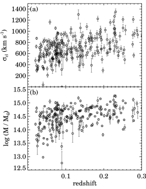
Figure 1.— (a) The velocity dispersion of HeCS-omnibus clusters as a function of cluster redshift. (b) The $M_{200}$ of the clusters based on the caustic technique as a function of cluster redshift.

3.3. Identification of the Brightest Cluster Galaxies

3.3.1 Identification of the BCGs

The BCG is the brightest galaxies in a cluster as the name suggests. Conventionally, BCGs are selected based on photometry (e.g. Lin, & Mohr, 2004; Lauer et al., 2014), although different photometric bands have been used. More recently, the galaxy with highest stellar mass among cluster members has been chosen as the BCG (e.g. Gozaliasl et al., 2019). This identification facilitates direct comparison with numerical simulations where the central galaxy presumably corresponds to the most massive subhalo in a cluster potential. However, identification of BCGs based on stellar mass may introduce uncontrolled systematics depending on the color and morphology of the galaxy.

Here, we define the BCG in the $r-$band. We additionally required that the BCG candidate be located within $0.5~{}R_{200}$. We apply this selection to reduce confusion resulting from bright galaxies outside the cluster center. Based on these two criteria, we first identify BCG candidates.

Some BCG candidates are not the actual BCG. These objects make the first cut due to imperfect SDSS photometry. Photometry of galaxies in crowded field is challenging because sky subtraction and masking of other objects are both difficult (e.g. Bernardi et al., 2010). Furthermore, Bernardi et al. (2013) show that the SDSS cModel magnitudes we use often overestimate the total magnitude of the object. They also demonstrated that the deviation is more significant for brighter galaxies in the cluster. These photometric issues can confuse BCG identification based on SDSS photometry.

For some BCGs, more recent SDSS photometry significantly overestimates the magnitudes. For example, Sohn et al. (2019) showed that the cModel magnitudes for the BCGs of A2029 and A2033 from SDSS DR12 photometry (similar to the DR14 photometry) are $\sim 3-4$ magnitude larger than those from SDSS DR7 photometry. The SDSS DR7 photometry is much better agreement with the luminosities of these BCGs in the literature (e.g. HyperLEDA, Makarov et al., 2014). In cases of large disagreement, the genuine BCGs can be misidentified.

We thus visually inspect BCG candidates based on the SDSS images. We update the BCG identification if there is an apparently brighter cluster member with incorrect SDSS photometry. There are $\sim 25$ HeCS-omnibus clusters with apparent BCGs that are inconsistent with the obvious brightest galaxy. Because these visually identified BCGs are bigger, brighter and closer to the cluster center, we also refine the visual identification.

3.3.2 HeCS-omnibus BCG Catalog

Table 3 lists the BCGs of the 220 HeCS-omnibus clusters. We cannot identify BCGs for five clusters (A1986, A2537, MS2349+2929, Zw1478, MSPM06300) because the obvious BCGs have no spectroscopic redshifts. The table includes the SDSS object ID, R.A., Decl., redshift, and $r-$band magnitude of the BCGs. We also include the physical properties of the BCGs including $D_{n}4000$, stellar mass, and stellar velocity dispersion. We note that 171, 216, 180 BCGs have $D_{n}4000$, stellar mass, and stellar velocity dispersion measurements, respectively.

Figure 2 summarizes the BCG identification for HeCS-omnibus clusters: (a) the SDSS color-composite image of the BCG, (b) the spatial distribution of cluster members and the BCG with respect to the cluster center, (c) the g-r vs. r color-magnitude diagram, and (d) the R-v diagram of cluster members and the BCG. The multi-dimensional graphs confirm that the BCG is indeed the massive central galaxy in each HeCS-omnibus cluster. These multi-dimensional graphs for the entire HeCS-omnibus clusters are available in our webpage .

Table 3The BCGs of the HeCS-omnibus Clusters

Cluster ID	BCG Object ID	R.A.	Decl.	z	$r_{petro,0}$	$\log(M_{*}/M_{\odot})$	$\sigma_{*}$
		(J2000)	(J2000)				(km s-1)
MKW4	1237651735757455411	181.112774	1.895971	$0.0197\pm 0.0001$	$11.78\pm 0.01$	$11.65\pm 0.25$	$297\pm 3$
A1367	1237668293912690766	176.008980	19.949825	$0.0208\pm 0.0001$	$12.12\pm 0.02$	$11.58\pm 0.18$	$281\pm 4$
MKW11	1237661816564482150	202.339834	11.735109	$0.0229\pm 0.0001$	$13.13\pm 0.01$	$11.03\pm 0.19$	$-99\pm-99$
A779	1237661126155436164	139.945219	33.749742	$0.0230\pm 0.0001$	$12.10\pm 0.01$	$11.53\pm 0.22$	$-99\pm-99$
Coma	1237667444048723983	195.033862	27.976941	$0.0215\pm 0.0001$	$11.71\pm 0.01$	$11.47\pm 0.19$	$368\pm 5$

3.3.3 Comparison with Previous BCG Catalogs

We cross-check our BCG identification with previous BCG catalogs. Lin, & Mohr (2004) publish a catalog of BCGs in 93 clusters and groups. There are 29 HeCS-omnibus clusters that overlap with Lin, & Mohr (2004) and 27 BCGs correspond exactly to the BCGs identified in Lin, & Mohr (2004). We identify different BCGs for two clusters: A2065 and A2147. In both cases, the BCGs identified by Lin, & Mohr (2004) are not coincident with the cluster center ($R_{cl}>0.7R_{200}$).

The BCG catalog from Lauer et al. (2014) includes 49 HeCS-omnibus clusters. We select different galaxies as BCGs for five of their clusters: A1066, A1436, A2065, A267, and A602. We inspect these difference in BCG identification based on location, magnitude, and morphology of the previously selected BCGs. The BCGs we identify are either brighter or they are located closer to the cluster center than the previously identified object. We also compare with the BCG catalog from Kluge et al. (2019) that includes 170 BCGs. Among 42 matched clusters, the BCGs of six clusters (A1066, A1423, A2065, A2199, A602, MKW4) are inconsistent. Again, the BCGs we identify are closer to the caustic center than the galaxies identified in Kluge et al. (2019).

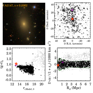
Figure 2.— Sample plots summarizing BCG identification for A2147. (Upper left) The SDSS color-composite image of the A2147 BCG (FoV: $20\arcsec\times 20\arcsec$). (Upper right) The spatial distribution of galaxies around the cluster center. Gray squares are the galaxies with spectroscopic redshifts and black circles are the spectroscopic members. The contours show the number density map of spectroscopic members of the cluster. The red star marks the BCG. The magenta cross shows the BCG identified by Lin, & Mohr (2004) or Lauer et al. (2014), if any. (Lower left) $g-r$ vs. $r$ color magnitude diagram of the cluster field. Symbols are the same as in the upper right panel. (Lower right) The R-v diagram of the cluster field. The solid lines show the caustic pattern for the cluster.

3.3.4 Properties of the BCGs

We examine the physical properties of the BCGs including $D_{n}4000$, stellar mass, and central velocity dispersion. For comparison, we investigate the properties of SDSS field galaxies. The field comparison sample is from the SDSS spectroscopic galaxy sample with magnitude limit $r<17.77$ and redshift range $z<0.1$. We obtain $D_{n}4000$, stellar mass, and the central velocity dispersions from the Portsmouth reduction.

Figure 3 displays the $D_{n}4000$ distributions of the BCGs and the SDSS field galaxies. The BCG $D_{n}4000$ distribution clearly differs from field. The majority of the BCGs ($\sim 95\%$) are quiescent galaxies with $D_{n}4000>1.5$. Unlike the BCGs, SDSS field galaxies show an obvious bimodal distribution. Furthermore, the field quiescent population shows a peak at $D_{n}4000\sim 1.85$, but the BCG population shows a peak at $D_{n}4000\sim 2.0$ with a typical uncertainty of 0.03. This comparison suggests that the stellar population of the central region of BCG is old.

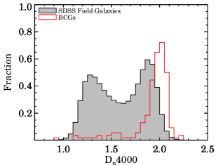
Figure 3.— The $D_{n}4000$ distributions of the HeCS-omnibus BCGs (open histogram) and SDSS field galaxies (filled histogram).

Figure 4 shows the central velocity dispersion as a function of stellar mass for BCGs. Most of the BCGs have high stellar mass ($>10^{11.5}M_{\odot}$) and high velocity dispersion ($>250~{}\rm km~{}s^{-1}$). We also plot the quiescent population in the SDSS field sample with $D_{n}4000>1.5$. The solid line in Figure 4 indicates the mean relation for SDSS field quiescent galaxies and the dashed (dotted) lines show the boundaries that include 68% (95%) of field galaxies. The comparison clearly shows that the BCGs represent the most massive tail of the population in terms of both stellar mass and velocity dispersion. Interestingly, the BCGs do follow the relation between stellar velocity dispersion and stellar mass defined by other quiescent galaxies.

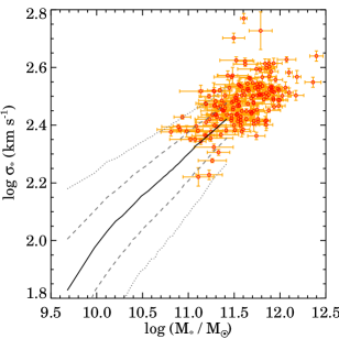
Figure 4.— Central velocity dispersion vs. stellar mass for the HeCS-omnibus BCGs (red circles). The solid line is the same relation for SDSS galaxies. The dashed and dotted lines include the 68% and 95% for SDSS galaxies.

4. Connection between BCGs and Clusters

The HeCS-omnibus clusters provide a basis for examining relations between BCG properties and the dynamical properties of their host clusters. We use absolute magnitude, stellar mass, and stellar velocity dispersion as mass proxies for the BCGs. We also use the cluster velocity dispersion and caustic mass (dynamical mass) for probing cluster properties. Here we explore the relations among these properties.

Figure 5 (a) shows the absolute magnitude of BCGs in the $r-$band as a function of redshift. Overall, BCGs are very bright ($M_{r}<-23$) over the entire range. Less luminous BCGs are mainly located in low redshift clusters. These low redshift clusters are also less massive than higher redshift systems (Figure 1).

Figures 5 (b) and (c) show the absolute magnitudes of BCGs as a function of $\sigma_{cl}$ and $M_{200}$. The clusters with higher velocity dispersion and higher dynamical mass host the brighter BCGs, consistent with previous studies (e.g. Lin, & Mohr, 2004). The Spearman rank correlation coefficients for these relations are 0.47 and 0.45 with significance of $2.66\times 10^{-13}$ and $2.36\times 10^{-12}$, respectively.

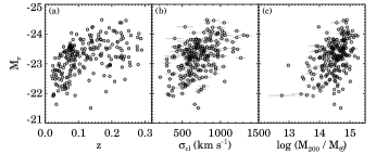
Figure 5.— $r-$band absolute magnitudes of BCGs as a function of cluster (a) redshift, (b) velocity dispersion, and (c) $M_{200}$.

Figure 6 shows the same relations as Figure 5, but based on BCG stellar mass ($M_{*,BCG}$). Similar to Figure 5 (a), the high redshift clusters contain more massive BCGs because our sample includes more massive clusters at higher redshift. Figures 6 (b) and (c) indicate that more massive clusters tend to host more massive BCGs. The Spearman correlation coefficients for $M_{*,BCG}$ versus $\sigma_{cl}$ relation and for $M_{*,BCG}$ versus $M_{200}$ relation are 0.34 and 0.34 with the significance of $3.32\times 10^{-7}$ and $3.24\times 10^{-7}$, respectively. Note that this correlation is somewhat weaker than the correlation between $M_{r}$ and the global cluster properties.

Previous observations show similar relations based on various cluster samples covering wide mass and redshift ranges (Kravtsov et al., 2018; Oliva-Altamirano et al., 2014; Erfanianfar et al., 2019). Most recently, Erfanianfar et al. (2019) investigated the connection between the stellar mass of the BCG and the cluster halo mass based on a large sample of 526 clusters within $0.1<z<0.65$. They estimated the halo mass of a cluster based on X-ray luminosity and the scaling relation between $M_{200}$ and the X-ray luminosity. They derived a best-fit relation between the BCG stellar mass and the cluster halo mass in two samples covering the redshift ranges ($0.1\leq z\leq 0.3$ and $0.3<z\leq 0.65$). They demonstrated that more massive clusters tend to have more massive BCGs. Furthermore, there is no significant redshift dependence for this relation. The blue dashed line in Figure 6 (c) displays the relation from Erfanianfar et al. (2019) for clusters in the redshift range ($0.1\leq z\leq 0.3$) similar to the HeCS-omnibus clusters.

To compare with previous results, we derive the best-fit relation based on a Markov chain Monte Carlo (MCMC) approach. We take the uncertainties in both variables into account and we assume that the uncertainties follow a 2D Gaussian. The best-fit relation (red solid line in Figure 6 (c)) between the BCG stellar mass and the cluster dynamical mass is:

$$\log(M_{*,BCG}/M_{\odot})=(0.46\pm 0.03)\log(M_{200,cl}/M_{\odot})+(5.05\pm 2.17).$$ (1)

The slope of the relation is consistent with the relations in the literature: e.g. $0.32\pm 0.09$ from Oliva-Altamirano et al. (2014) and $0.41\pm 0.04$ from Erfanianfar et al. (2019).

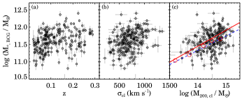
Figure 6.— Stellar masses of the BCGs as a function of (a) redshift, (b) $\sigma_{cl}$, and (c) $M_{200}$. In panel (c), the dashed line shows the BCG stellar mass - cluster halo mass relation from Erfanianfar et al. (2019). The solid line displays the best-fit relation we derive for the HeCS-omnibus clusters.

Figure 7.— Stellar velocity dispersion of BCGs as a function of cluster (a) redshift, (b) $\sigma_{cl}$, and (c) $M_{200}$. The red solid lines in panel (b) and (c) show the best-fit power law for the BCG stellar velocity dispersion and the cluster halo mass. The blue dashed lines are the prediction from numerical simulations in Dolag et al. (2010) (see Section 5).

In Figure 7, we explore the relation between the BCG stellar velocity dispersion ($\sigma_{*,BCG}$) and the cluster (a) redshift, (b) $\sigma_{cl}$, and (c) $M_{200}$. Interestingly, $\sigma_{*,BCG}$ correlates well with $\sigma_{cl}$ and with $M_{200}$. These correlations are expected because the stellar velocity dispersion of the central galaxy is a good tracer of its halo mass (e.g. Wake et al., 2012; Zahid et al., 2016, 2018).

Even though the dynamic range of the BCG stellar velocity dispersion is small, the relation between $\sigma_{*,BCG}$ and $\sigma_{cl}$ is remarkably tight (Figure 7 (b)). The Spearman rank correlation coefficient is 0.42 with a significance of $3.95\times 10^{-8}$. The best-fit relation (the red solid line) for these variables based on the MCMC approach is

$$\log\sigma_{*,BCG}=(0.46\pm 0.09)~{}\log\sigma_{cl}+(1.16\pm 3.45).$$ (2)

For the first time, Figure 7 (c) shows that $\sigma_{*,BCG}$ correlates well with the cluster mass based on a large dataset. The Spearman rank correlation coefficient for this relation is 0.38 with a significance of $1.27\times 10^{-6}$. The best-fit relation (the red solid line) from the MCMC approach is

$$\log\sigma_{*,BCG}=(0.13\pm 0.01)~{}\log(M_{200,cl}/M_{\odot})+(0.61\pm 3.19).$$ (3)

The blue dashed line in Figures 7 (b) and (c) display the expected relations based on cosmological hydrodynamic simulations from Dolag et al. (2010). We compare with the Dolag et al. (2010) simulations because they are unique in examining the relations between BCG velocity dispersion, cluster velocity dispersion, and halo mass. The typical mass resolution of their simulations is $3.1\times 10^{9}h^{-1}~{}M_{\odot}$ for dark matter particle and $0.48\times 10^{9}h^{-1}~{}M_{\odot}$ for gas particle. The simulation uses a smoothed particle hydrodynamics and takes radiative cooling, heating by a UV background, star formation and feedback into account . Based on the modified SUBFIND algorithm (Springel et al., 2001; Dolag et al., 2009), they identified 44 clusters with more than 20 satellite galaxies. There are star particles not bound to any subhalo within the cluster potential. These star particles are either the stellar component of the BCG (cD galaxy) or a diffuse stellar component (DSC). Dolag et al. (2010) separated these two components based on velocity histograms and derived the velocity dispersion of each of these two components. From a Maxwellian fit to the two differerent stellar components, they compute the velocity dispersion of the BCG and the DSC.

The observed data scatter around the predicted relation from the numerical simulation. We note that the BCG velocity dispersion estimates from Dolag et al. (2010), the Maxwellian fit to the BCG stellar component, are not identical to our stellar velocity dispersion estimates. Dolag et al. (2010) also used the virial mass; we use a proxy for the virial mass, $M_{200}$. Therefore, differences in the slope of the relations in Figure 7 (c) may result from the different definition of the velocity dispersion and the cluster mass. Despite the different slopes, both observation and simulation demonstrate that the stellar velocity dispersion correlates well with the cluster mass. Furthermore, the tight relation suggests that the stellar velocity dispersion of the BCGs is a good halo mass predictor in analogy with the stellar mass (Pillepich et al., 2018).

5. COMPARISON WITH SIMULATIONS

Based on 227 HeCS-omnibus clusters, we explore the relation between the BCGs and their host clusters. We use three different mass proxies for the BCGs including absolute magnitude, stellar mass, and the stellar velocity dispersion. We also use the cluster velocity dispersion ($\sigma_{cl}$) and the cluster dynamical mass ($M_{200}$) measured from the caustic technique to probe the cluster halo mass. In general, more massive cluster contain the more massive BCGs. Particularly, the BCG stellar velocity dispersion ($\sigma_{*,BCG}$) show a tight relation with cluster halo mass proxies. Here, we compare the observed relations with predictions from numerical simulations. In Section 5.1, we compare the observed and predicted relations for $M_{*,BCG}$ and $M_{200}$. We also investigate the relations between $\sigma_{*,BCG}$ and $\sigma_{cl}$, a distinctive comparison based on the HeCS-omnibus sample (5.2).

5.1. $M_{*,BCG}$ vs. $M_{200}$ Relations

The stellar mass of BCGs in the HeCS-omnibus clusters is correlated with the cluster mass. This observed relation is consistent with results from previous observations based on different cluster samples over a wide redshift range. The relation between $M_{*,BCG}$ and $M_{200}$ provides a testbed for modeling the formation and evolution of galaxy and its halo.

Another important relation to test is the ratio between BCG stellar mass and the cluster halo mass as a function of halo mass. Figure 8 illustrates this relation based on BCG stellar mass ($M_{*,BCG}$) and the cluster dynamical mass ($M_{200}$). The observed relation for the HeCS-omnibus clusters shows a tight negative correlation; the Spearman correlation coefficient is -0.68 with a significance of $1.35\times 10^{-30}$. The best-fit relation based on the MCMC approach is:

$$\log(M_{*,BCG}/M_{200})=(-0.77\pm 0.12)\log M_{200}+(8.39\pm 4.05).$$ (4)

For comparison, we plot the same relation from Erfanianfar et al. (2019) (blue dotted line). Erfanianfar et al. (2019) estimated the stellar mass based on SDSS, Galaxy Evolution Explorer (GALEX), and Wide-Field Infrared Survey Explorer (WISE) photometry using Le Phare. They converted cluster X-ray luminosity into the $M_{200}$ based on a scaling relation from Leauthaud et al. (2010). Therefore, the slight differences result from the different definitions of $M_{200}$ and the different photometry used for stellar mass estimation.

Figure 8.— Ratio between the BCG stellar mass ($M_{*,BCG}$) and the cluster dynamical mass ($M_{200}$) as a function of cluster dynamical mass ($M_{200}$). The red solid line shows the best-fit relation to the HeCS-omnibus sample. The green dash-dotted line indicates the best-fit relation for the clusters at $0.1<z<0.3$ from Erfanianfar et al. (2019). The blue dashed line shows the relation from empirical models of Behroozi et al. (2019).

We also compare the relation from UNIVERSEMACHINE (Behroozi et al., 2019), an empirical model that traces galaxy evolution based on dark matter halo evolution. This model is constrained by various observed relations including environmental effects on star formation rate of a galaxy. This model provides a stellar mass to halo mass relation for quiescent central galaxies as a function of redshift. We compute the relation from UNIVERSEMACHINE (blue dashed line in Figure 8) at the median redshift of HeCS-omnibus clusters, i.e. $z=0.1$. The model relation shows a slightly different slope and differs from the observed relation especially at large $M_{200}$ where the data barely overlap with the model.

5.2. $\sigma_{*,BCG}$ vs. $\sigma_{cl}$ Relations

Based on the extensive dataset for $\sigma_{*,BCG}$, $\sigma_{cl}$, and $M_{200}$ for the HeCS-omnibus clusters, we compare the observed relations among these variables with the same relations from the numerical simulations of Dolag et al. (2010). Similar to $M_{*,BCG}$, $\sigma_{*,BCG}$ shows a good correlation with both $\sigma_{cl}$ and $M_{200}$. One interesting point is that the measured $\sigma_{*,BCG}$ is generally below $\sigma_{cl}$ as in the simulations. Dolag et al. (2010) conclude that $\sigma_{*,BCG}$ is governed by the local galactic potential rather than by the global cluster potential. The observed relation supports this idea.

Figure 9 demonstrates that the ratio between $\sigma_{*,BCG}$ and $\sigma_{cl}$ decreases as a function of $\sigma_{cl}$. These two variables show a remarkable tight negative correlation (tighter than the $M_{*,BCG}/M_{200}$ vs. $M_{200}$ relation); the Spearman rank correlation coefficient is -0.79 with a significance of $1.93\times 10^{-35}$. The best-fit relation (the red solid line) based on the MCMC approach is

$$\sigma_{*,BCG}/\sigma_{cl}=(-0.82\pm 0.17)\log\sigma_{cl}+(2.77\pm 3.93).$$ (5)

This relation indicates that the fraction of mass enclosed in the BCG subhalo continuously decreases as the cluster mass increases.

Unlike the observed relation, the Dolag et al. (2010) simulation suggests a constant ratio between $\sigma_{*,BCG}$ and $\sigma_{cl}$ over a wide range of $\sigma_{cl}$. In Figure 9, the blue solid and dashed lines show the relation and $1\sigma$ deviation from the simulation. In this simulation, the velocity dispersion of the BCGs, DSC, and cluster galaxies correlate well with the virial mass of the cluster halo. The cluster halo mass is proportional to $\sigma^{3}$ although the normalization varies with the particular source of the velocity dispersion (i.e. $\sigma_{*,BCG},\sigma_{DSC}$ and $\sigma_{cl}$), Thus, the $\sigma_{*,BCG}/\sigma_{cl}$ ratio does not change as a function of $\sigma_{cl}$.

The observed $\sigma_{*,BCG}/\sigma_{cl}$ does depend on cluster mass and suggests that the mass fraction associated with the BCGs reflects the evolution of the BCGs and their host halo. The high mass clusters are presumably developed systems and their central BCGs have only experienced minor interactions very recently. Thus, the center of the BCGs are relaxed and the BCG velocity dispersion has not increased with the cluster velocity dispersion. Indeed, Edwards et al. (2019) show that the core region of the BCG formed very early ($>13$ Gyrs ago) based on the Integral Field Unit (IFU) observations of BCGs in massive clusters. In contrast, galaxies in lower mass clusters encounter one another at relatively low velocities. The low relative velocities among members result in a merging instability among member galaxies. In these systems, the BCGs can grow more efficiently through more major mergers.

The observed relation between $\sigma_{*,BCG}$ and $\sigma_{cl}$ promises an important test of galaxy and cluster formation models. Many previous studies focused instead on the stellar mass of the BCGs. Compared with the BCG stellar mass, the BCG velocity dispersion measurement from numerical simulations is insensitive to systematic biases introduced by various baryonic physics inserted in the simulations including feedback models. From theoretical point of view the BCG velocity dispersion is also less sensitive to systematics than the stellar mass. The BCG velocity dispersion is a strong test of the physics of BCG formation.

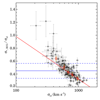
Figure 9.— Ratio between the BCG stellar velocity dispersion ($\sigma_{*,BCG}$) and the cluster velocity dispersion ($\sigma_{cl}$) as a function of cluster velocity dispersion ($\sigma_{cl}$). Red square are the median $\sigma_{*,BCG}/\sigma_{cl}$ ratio in various $\sigma_{cl}$ bins. The red dashed line shows the best-fit relation to the HeCS-omnibus sample. The blue solid line shows the expected ratio from the cosmological hydrodynamic simulations by Dolag et al. (2010); the blue dashed lines are the $1\sigma$ boundaries for the expected ratio.

6. CONCLUSION

HeCS-omnibus is a new cluster data compilation including 227 clusters covering the range $0.02<z<0.29$ with $\sim 180$ spectroscopic members per cluster. We obtained the spectroscopic survey data mainly from MMT/Hectospec and the SDSS. Each of the HeCS-omnibus clusters typically includes $\sim 180$ spectroscopic members.

We derive physical properties of the cluster galaxies including absolute magnitude, $D_{n}4000$, stellar mass, and stellar velocity dispersion. We also compute velocity dispersions and dynamical masses of the HeCS-omnibus clusters based on spectroscopic members. We identify the BCGs based on multi-dimensional data including the spatial distribution and R-v diagram of spectroscopic members.

The BCG properties correlate with the mass of the host clusters; more massive clusters tend to have brighter, more massive BCGs. These relations for HeCS-omnibus clusters are consistent with previous observations (Kravtsov et al., 2018; Erfanianfar et al., 2019). However, we note that the luminosity and the stellar mass of the BCGs suffer from systematic issues due to problematic photometry in crowded region like cluster cores (e.g. Bernardi et al., 2013).

The BCG stellar velocity dispersion ($\sigma_{*,BCG}$) show a remarkably tight correlation with host cluster mass proxies ($\sigma_{cl}$ and $M_{200}$). This observed relation is consistent with predictions of the numerical simulation of Dolag et al. (2010). The tight relation suggests that $\sigma_{cl}$ of a BCG is a good tracer of the cluster halo mass as well as of the BCG stellar mass.

The hierarchical structure formation model predicts a connection between the (stellar) mass of the central galaxy and the cluster halo mass (e.g. De Lucia & Blaizot, 2007; Pillepich et al., 2018; Ragone-Figueroa et al., 2018). A simple explanation for this connection is that the massive cluster has experienced more accretion (or mergers) and thus its BCG accretes more mass. Indeed, many numerical simulations suggest that the mass growth of the BCG is dominated by accretion rather than in situ star formation (De Lucia & Blaizot, 2007; Ragone-Figueroa et al., 2018; Pillepich et al., 2018).

Many previous studies have investigated the connection between BCG and cluster halo masses using simulations and observations, but most studies are based on the stellar mass. Our results suggest that the stellar velocity dispersion provide an additional important constraint on this connection. Unlike the stellar mass estimates, stellar velocity dispersion is relatively insensitive to systematic issues introduced by photometry in crowded region and or on the assumptions for stellar population models. Once the stellar velocity dispersion is measured in simulations using the observational procedure we use (Zahid et al., 2018), the central velocity dispersions of the BCG has the potential to provide additional powerful constraints on formation models.

We demonstrate that the ratio between the BCG and cluster velocity dispersions, $\sigma_{*,BCG}/\sigma_{cl}$, decreases as $\sigma_{cl}$ increases. This observed relation suggests that the mass assembly of the BCG subhalo changes in a way that correlates closely with the cluster mass and its accretion history. The observed trend is similar to the relation between $M_{*,BCG}/M_{200}$ and $M_{200}$ shown in previous observational and theoretical works (Kravtsov et al., 2018; Erfanianfar et al., 2019; Pillepich et al., 2018; Behroozi et al., 2019). Nonetheless, the $\sigma_{*,BCG}/\sigma_{cl}$ ratio trend differs from the theoretical prediction of Dolag et al. (2010) suggesting that the BCG growth is more efficient in lower mass systems. Further tests of $\sigma_{*,BCG}$ and $\sigma_{cl}$ in large-scale numerical simulations will be useful for understanding the apparent change in BCG formation efficiency with the cluster mass (and velocity dispersion).

References

- Abell (1958) Abell, G. O. 1958, ApJS, 3, 211
- Abell et al. (1989) Abell, G. O., Corwin, H. G., & Olowin, R. P. 1989, ApJS, 70, 1
- Arnouts et al. (1999) Arnouts, S., Cristiani, S., Moscardini, L., et al. 1999, MNRAS, 310, 540
- Baldwin et al. (1981) Baldwin, J. A., Phillips, M. M., & Terlevich, R. 1981, PASP, 93, 5
- Balogh et al. (1999) Balogh, M. L., Morris, S. L., Yee, H. K. C., et al. 1999, ApJ, 527, 54
- Beers et al. (1990) Beers, T. C., Flynn, K., & Gebhardt, K. 1990, AJ, 100, 32
- Behroozi et al. (2010) Behroozi, P. S., Conroy, C., & Wechsler, R. H. 2010, ApJ, 717, 379
- Behroozi et al. (2019) Behroozi, P., Wechsler, R. H., Hearin, A. P., et al. 2019, MNRAS, 488, 3143
- Bernardi et al. (2010) Bernardi, M., Shankar, F., Hyde, J. B., et al. 2010, MNRAS, 404, 2087
- Bernardi et al. (2013) Bernardi, M., Meert, A., Sheth, R. K., et al. 2013, MNRAS, 436, 697
- Biviano (2000) Biviano, A. 2000, Constructing the Universe with Clusters of Galaxies, 1
- Bruzual, & Charlot (2003) Bruzual, G., & Charlot, S. 2003, MNRAS, 344, 1000
- Calzetti et al. (2000) Calzetti, D., Armus, L., Bohlin, R. C., et al. 2000, ApJ, 533, 682
- Cappellari & Emsellem (2004) Cappellari, M., & Emsellem, E. 2004, PASP, 116, 138
- Cardelli et al. (1989) Cardelli, J. A., Clayton, G. C., & Mathis, J. S. 1989, ApJ, 345, 245
- Chabrier (2003) Chabrier, G. 2003, PASP, 115, 763
- Conroy et al. (2006) Conroy, C., Wechsler, R. H., & Kravtsov, A. V. 2006, ApJ, 647, 201
- Coziol et al. (2009) Coziol, R., Andernach, H., Caretta, C. A., et al. 2009, AJ, 137, 4795
- De Lucia & Blaizot (2007) De Lucia, G., & Blaizot, J. 2007, MNRAS, 375, 2
- Diaferio & Geller (1997) Diaferio, A., & Geller, M. J. 1997, ApJ, 481, 633
- Diaferio (1999) Diaferio, A. 1999, MNRAS, 309, 610
- Dolag et al. (2009) Dolag, K., Borgani, S., Murante, G., et al. 2009, MNRAS, 399, 497
- Dolag et al. (2010) Dolag, K., Murante, G., & Borgani, S. 2010, MNRAS, 405, 1544
- Edwards et al. (2019) Edwards, L. O. V., Salinas, M., Stanley, S., et al. 2019, MNRAS, 2328
- Erfanianfar et al. (2019) Erfanianfar, G., Finoguenov, A., Furnell, K., et al. 2019, arXiv e-prints, arXiv:1908.01559
- Evrard et al. (2008) Evrard, A. E., Bialek, J., Busha, M., et al. 2008, ApJ, 672, 122
- Faber & Jackson (1976) Faber, S. M., & Jackson, R. E. 1976, ApJ, 204, 668
- Fabricant et al. (2005) Fabricant, D., Fata, R., Roll, J., et al. 2005, PASP, 117, 1411
- Fabricant et al. (2013) Fabricant, D., Chilingarian, I., Hwang, H. S., et al. 2013, PASP, 125, 1362
- Fakhouri et al. (2010) Fakhouri, O., Ma, C.-P., & Boylan-Kolchin, M. 2010, MNRAS, 406, 2267
- Gao et al. (2012) Gao, L., Navarro, J. F., Frenk, C. S., et al. 2012, MNRAS, 425, 2169
- Gonzalez et al. (2007) Gonzalez, A. H., Zaritsky, D., & Zabludoff, A. I. 2007, ApJ, 666, 147
- Gozaliasl et al. (2019) Gozaliasl, G., Finoguenov, A., Tanaka, M., et al. 2019, MNRAS, 483, 3545
- Gullieuszik et al. (2015) Gullieuszik, M., Poggianti, B., Fasano, G., et al. 2015, A&A, 581, A41
- Guo et al. (2010) Guo, Q., White, S., Li, C., et al. 2010, MNRAS, 404, 1111
- Haines et al. (2018) Haines, C. P., Finoguenov, A., Smith, G. P., et al. 2018, MNRAS, 477, 4931
- Hao et al. (2010) Hao, J., McKay, T. A., Koester, B. P., et al. 2010, ApJS, 191, 254
- Habas et al. (2018) Habas, R., Fadda, D., Marleau, F. R., et al. 2018, MNRAS, 475, 4544
- Haines et al. (2013) Haines, C. P., Pereira, M. J., Smith, G. P., et al. 2013, ApJ, 775, 126
- Hwang et al. (2010) Hwang, H. S., Elbaz, D., Lee, J. C., et al. 2010, A&A, 522, A33
- Hwang et al. (2012) Hwang, H. S., Geller, M. J., Diaferio, A., et al. 2012, ApJ, 752, 64
- Ilbert et al. (2006) Ilbert, O., Arnouts, S., McCracken, H. J., et al. 2006, A&A, 457, 841
- Illingworth (1976) Illingworth, G. 1976, ApJ, 204, 73
- Kauffmann et al. (2003) Kauffmann, G., Heckman, T. M., White, S. D. M., et al. 2003, MNRAS, 341, 33
- Kauffmann et al. (2003) Kauffmann, G., Heckman, T. M., Tremonti, C., et al. 2003, MNRAS, 346, 1055
- Kewley et al. (2001) Kewley, L. J., Dopita, M. A., Sutherland, R. S., et al. 2001, ApJ, 556, 121
- Kluge et al. (2019) Kluge, M., Neureiter, B., Riffeser, A., et al. 2019, arXiv e-prints, arXiv:1908.08544
- Koester et al. (2007) Koester, B. P., McKay, T. A., Annis, J., et al. 2007, ApJ, 660, 239
- Koleva et al. (2009) Koleva, M., Prugniel, P., Bouchard, A., et al. 2009, A&A, 501, 1269
- Kravtsov, & Borgani (2012) Kravtsov, A. V., & Borgani, S. 2012, ARA&A, 50, 353
- Kravtsov et al. (2018) Kravtsov, A. V., Vikhlinin, A. A., & Meshcheryakov, A. V. 2018, Astronomy Letters, 44, 8
- Kurtz, & Mink (1998) Kurtz, M. J., & Mink, D. J. 1998, PASP, 110, 934
- Lauer et al. (2014) Lauer, T. R., Postman, M., Strauss, M. A., et al. 2014, ApJ, 797, 82
- Leauthaud et al. (2010) Leauthaud, A., Finoguenov, A., Kneib, J.-P., et al. 2010, ApJ, 709, 97
- Leauthaud et al. (2012) Leauthaud, A., Tinker, J., Bundy, K., et al. 2012, ApJ, 744, 159
- Lin, & Mohr (2004) Lin, Y.-T., & Mohr, J. J. 2004, ApJ, 617, 879
- Mahdavi & Geller (2001) Mahdavi, A., & Geller, M. J. 2001, ApJ, 554, L129
- Makarov et al. (2014) Makarov, D., Prugniel, P., Terekhova, N., et al. 2014, A&A, 570, A13
- Maraston & Strömbäck (2011) Maraston, C., & Strömbäck, G. 2011, MNRAS, 418, 2785
- Matthews et al. (1964) Matthews, T. A., Morgan, W. W., & Schmidt, M. 1964, ApJ, 140, 35
- McBride et al. (2009) McBride, J., Fakhouri, O., & Ma, C.-P. 2009, MNRAS, 398, 1858
- McNamara & Nulsen (2007) McNamara, B. R., & Nulsen, P. E. J. 2007, ARA&A, 45, 117
- Moretti et al. (2017) Moretti, A., Gullieuszik, M., Poggianti, B., et al. 2017, A&A, 599, A81
- Morgan (1958) Morgan, W. W. 1958, PASP, 70, 364
- Moster et al. (2010) Moster, B. P., Somerville, R. S., Maulbetsch, C., et al. 2010, ApJ, 710, 903
- Moster et al. (2018) Moster, B. P., Naab, T., & White, S. D. M. 2018, MNRAS, 477, 1822
- Newman et al. (2013) Newman, A. B., Treu, T., Ellis, R. S., et al. 2013, ApJ, 765, 25
- Pillepich et al. (2018) Pillepich, A., Nelson, D., Hernquist, L., et al. 2018, MNRAS, 475, 648
- Ragone-Figueroa et al. (2018) Ragone-Figueroa, C., Granato, G. L., Ferraro, M. E., et al. 2018, MNRAS, 479, 1125
- Rines & Diaferio (2006) Rines, K., & Diaferio, A. 2006, AJ, 132, 1275
- Rines et al. (2013) Rines, K., Geller, M. J., Diaferio, A., et al. 2013, ApJ, 767, 15
- Rines et al. (2016) Rines, K. J., Geller, M. J., Diaferio, A., et al. 2016, ApJ, 819, 63
- Rines et al. (2018) Rines, K. J., Geller, M. J., Diaferio, A., et al. 2018, ApJ, 862, 172
- Rines et al. (in preparation) Rines, K. J., Geller, M. J., Diaferio, A., et al. 2020
- Rykoff et al. (2014) Rykoff, E. S., Rozo, E., Busha, M. T., et al. 2014, ApJ, 785, 104
- Silk, & Rees (1998) Silk, J., & Rees, M. J. 1998, A&A, 331, L1
- Oliva-Altamirano et al. (2014) Oliva-Altamirano, P., Brough, S., Lidman, C., et al. 2014, MNRAS, 440, 762
- Osterbrock & Ferland (2006) Osterbrock, D. E., & Ferland, G. J. 2006, Astrophysics of gaseous nebulae and active galactic nuclei
- Saro et al. (2013) Saro, A., Mohr, J. J., Bazin, G., et al. 2013, ApJ, 772, 47
- Serra et al. (2011) Serra, A. L., Diaferio, A., Murante, G., et al. 2011, MNRAS, 412, 800
- Serra, & Diaferio (2013) Serra, A. L., & Diaferio, A. 2013, ApJ, 768, 116
- Springel et al. (2001) Springel, V., White, S. D. M., Tormen, G., et al. 2001, MNRAS, 328, 726
- Sohn et al. (2017) Sohn, J., Geller, M. J., Zahid, H. J., et al. 2017, ApJS, 229, 20
- Sohn et al. (2019) Sohn, J., Geller, M. J., Zahid, H. J., et al. 2019, ApJ, 872, 192
- Sohn et al. (2019) Sohn, J., Geller, M. J., & Zahid, H. J. 2019, ApJ, 880, 142
- Sohn et al. (in preparation) Sohn, J., Geller, M. J., Diaferio, A., et al. 2020
- Thomas et al. (2013) Thomas, D., Steele, O., Maraston, C., et al. 2013, MNRAS, 431, 1383
- van den Bosch (2002) van den Bosch, F. C. 2002, MNRAS, 331, 98
- van Uitert et al. (2013) van Uitert, E., Hoekstra, H., Franx, M., et al. 2013, A&A, 549, A7
- Vogelsberger et al. (2014) Vogelsberger, M., Genel, S., Springel, V., et al. 2014, MNRAS, 444, 1518
- Wake et al. (2012) Wake, D. A., van Dokkum, P. G., & Franx, M. 2012, ApJ, 751, L44
- Wang et al. (2006) Wang, L., Li, C., Kauffmann, G., et al. 2006, MNRAS, 371, 537
- Wechsler & Tinker (2018) Wechsler, R. H., & Tinker, J. L. 2018, ARA&A, 56, 435
- Zahid et al. (2016) Zahid, H. J., Geller, M. J., Fabricant, D. G., et al. 2016, ApJ, 832, 203
- Zahid & Geller (2017) Zahid, H. J., & Geller, M. J. 2017, ApJ, 841, 32
- Zahid et al. (2018) Zahid, H. J., Sohn, J., & Geller, M. J. 2018, ApJ, 859, 96
- Zhang et al. (2011) Zhang, Y.-Y., Andernach, H., Caretta, C. A., et al. 2011, A&A, 526, A105
- Zhao et al. (2009) Zhao, D. H., Jing, Y. P., Mo, H. J., et al. 2009, ApJ, 707, 354