Analytical Theory for Sequence-Specific Binary Fuzzy Complexes of Charged Intrinsically Disordered Proteins

Abstract

Intrinsically disordered proteins (IDPs) are important for biological functions. In contrast to folded proteins, molecular recognition among certain IDPs is “fuzzy” in that their binding and/or phase separation are stochastically governed by the interacting IDPs’ amino acid sequences while their assembled conformations remain largely disordered. To help elucidate a basic aspect of this fascinating yet poorly understood phenomenon, the binding of a homo- or hetero-dimeric pair of polyampholytic IDPs is modeled statistical mechanically using cluster expansion. We find that the binding affinities of binary fuzzy complexes in the model correlate strongly with a newly derived simple “jSCD” parameter readily calculable from the pair of IDPs’ sequence charge patterns. Predictions by our analytical theory are in essential agreement with coarse-grained explicit-chain simulations. This computationally efficient theoretical framework is expected to be broadly applicable to rationalizing and predicting sequence-specific IDP-IDP polyelectrostatic interactions.

1 Introduction

Intrinsically disordered proteins (IDPs)—hallmarked by their lack of folding to an essentially unique conformation in isolation—serve many physiological functions.^{1, 2} Compared to globular proteins, IDPs are depleted in nonpolar but enriched in polar, aromatic, and charged residues. ³ Some IDPs adopt ordered/folded conformations upon binding to folded targets ⁴ or after posttranslational modifications⁵, others remain disordered. Among the spectrum of diverse possible behaviors⁶, the IDPs in certain IDP-folded protein complexes can be highly disordered, as typified by the kinase inhibitor/ubiquitin ligase Sic1-Cdc4 complexes ^{7, 8}.

Complexes with bound IDPs that are disordered are aptly named “fuzzy complexes”^{9, 10, 11, 12}. The role of these IDPs’ amino acid sequences in molecular recognition varies, depending on the situation. For Sic1-Cdc4, most of the charges in the disordered Sic1 probably take part in modulating binding affinity via multiple spatially long-range electrostatic—termed polyelectrostatic⁷—interactions with the folded Cdc4 without locally engaging the Cdc4 binding pockets ^{8, 13}. In contrast, for the IDP transactivation domain of Ewing sarcoma, sequence-dependent oncogenic effects may be underpinned largely by multivalent, spatially short-range polycation-$\pi$ interactions implicating the IDP’s tyrosine residues ^{14, 15}. More broadly, for multiple-component phase separation of IDPs, a “fuzzy” mode of molecular recognition was proposed whereby mixing/demixing of phase-separated polyampholyte species depends on quantifiable differences in the IDPs’ sequence charge patterns ¹⁶. Variations aside, these mechanisms share the commonality of being stochastic in essence, involving highly dynamic conformations, and as such are distinct from those underlying the structurally specific and relatively static binding participated by folded proteins. We thus extend the usage of “fuzzy” as an adjective not only for the structural features of certain biomolecular assemblies but also for the molecular recognition mechanisms that contribute to the formation of fuzzy assemblies. This concept is applicable to nonbiological polymers as well. Whereas multivalency, stochasticity, and conformational diversity have long been the mainstay of polymer physics, recently, sequence specificity and therefore fuzzy molecular recognition has become increasingly important for nonbiological heteropolymers because of experimental advances in “monomer precision” that allows for the synthesis of sequence-monodisperse polymers ¹⁷.

As far as biomolecules are concerned, fuzzy molecular recognition should play a dominant role in “binding without folding” IDP complexes wherein the bound IDPs are disordered ^{18, 19}. Generally speaking, a condensed liquid droplet of IDP is a mesoscopic fuzzy assembly underpinned by a fuzzy molecular recognition mechanism.¹⁶ With regard to basic binary (two-chain) IDP complexes, evidence has long pointed to their existence,^{20, 21} although extra caution needed to be used to interpret the pertinent experimental data.^{22, 18} Of notable recent interest is the interaction between the strongly but oppositely charged H1 and ProT$\alpha$ IDPs involved in chromatin condensation and remodeling, which remain disorder while forming a heterodimer with reported dissociation constant ranging from nanomolar ²³ to sub-micromolar levels ²⁴.

We now tackle a fundamental aspect of fuzzy molecular recognition, namely the impact of sequence-specific electrostatics on binary fuzzy complexes. Electrostatics is important for IDP interactions^{7, 23, 25, 19} including phase separation.^{16, 26, 27} IDP sequence specificity is a key feature of their single-chain properties^{28, 29, 30, 31} and multiple-chain phase behaviors.^{32, 33, 34, 35, 36, 37, 38, 39, 40, 41} IDP properties depend not only on their net charge but are also sensitive, to various degrees, to their specific sequence charge pattern, which has been characterized by two parameters, $\kappa$ and “sequence charge decoration” (SCD): $\kappa$ is an intuitive blockiness measure²⁸; whereas

$$\text{SCD}(\{\sigma\})=\frac{1}{2N}\tsum\slimits@_{s,t=1}^{N}\sigma_{s}\sigma_{t}\sqrt{|s-t|}\;,$$ (1)

defined for any charge sequence $\{\sigma\}=\{\sigma_{1},\sigma_{2},\dots,\sigma_{N}\}$, emerges from an analytical theory for polyampholyte dimensions²⁹. Both single-chain dimensions^{28, 29, 30} and phase separation propensities^{30, 42, 38, 39, 41} are seen to correlate with these parameters. These measures are found to be evolutionarily conserved among IDPs, suggesting intriguingly that the gestalt properties they capture are functionally significant ⁴³. Our present focus is on binary complexes, which are of interest themselves²³ and possibly also as proxies for mesoscopic multiple-IDP phase behaviors. Generalizing such a correspondence between single-chain properties and multiple-chain phase behaviors for homopolymers ^{44, 45} and polyampholytes ³⁰, for example, the osmotic second virial coefficient, $B_{2}$, of a pair of IDP chains has been proposed as an approximate measure for the IDP’s sequence-dependent phase separation propensity ⁴⁶.

2 Methods

With these thoughts in mind, we develop an analytical theory for binary IDP-IDP electrostatics. As exemplified by recent studies of phase behaviors,^{33, 35, 47} approximate analytical theories, among complementary approaches, are conceptually productive and efficient for gaining insights into sequence-specific IDP behaviors. The system analyzed herein consists of two IDPs $A$, $B$ of lengths ${N_{A}}$, ${N_{B}}$; charge sequences $\{\sigma^{A}\}=\{\sigma^{A}_{1},\sigma^{A}_{2},\dots,\sigma^{A}_{{N_{A}}}\}$, $\{\sigma^{B}\}=\{\sigma^{B}_{1},\sigma^{B}_{2},\dots,\sigma^{B}_{{N_{B}}}\}$; and residue (monomer) coordinates $\{{\bf R}^{A}\}=\{{\bf R}_{1}^{A},{\bf R}_{2}^{A},\dots,{\bf R}_{{N_{A}}}^{A}\}$, $\{{\bf R}^{B}\}=\{{\bf R}_{1}^{B},{\bf R}_{2}^{B},\dots,{\bf R}_{{N_{B}}}^{B}\}$. Both $A=B$ (homotypic) and $A\ne B$ (heterotypic) cases are considered. Key steps in the formal development are presented below; details are provided in the Supporting Information. The second virial coefficient of the IDP pair is given by ⁴⁸

$$B_{2}=\int d{\bf R}_{\rm CM}^{AB}\;\left\langle 1-e^{-\beta\,{\cal U}^{AB}({\bf R}_{\rm CM}^{AB};\{{\bf R}^{A}\},\{{\bf R}^{B}\})}\right\rangle_{A,B}\;,$$ (2)

where $\beta=1/k_{\rm B}T$ ($k_{\rm B}$ is Boltzmann constant, $T$ is absolute temperature), ${\bf R}_{\rm CM}^{AB}$ is the center-of-mass distance and $\,{\cal U}^{AB}$ is the total interaction between $A$ and $B$, and the average $\left\langle\@cdots\right\rangle_{A,B}$ is over the conformational ensembles of $A$ and $B$. To simplify notation, we use $\,{\cal U}^{AB}$ to denote $\beta\,{\cal U}^{AB}$ below. Now, Eq. 2 may be rewritten as

$$B_{2}=V-\frac{{{\cal Q}_{A\!B}}}{{{\cal Q}_{A}}{{\cal Q}_{B}}}=V\int\mathscr{D}[{\bf R}^{A}]\mathscr{D}[{\bf R}^{B}]{\cal P}^{A}[{\bf R}^{A}]{\cal P}^{B}[{\bf R}^{B}]\left(1-e^{-\,{\cal U}^{AB}[{\bf R}^{A},{\bf R}^{B}]}\right)\;,$$ (3)

where $V$ is volume, ${{\cal Q}_{A\!B}}$ is the partition function of the entire $A$-$B$ system; ${{\cal Q}_{A}}$ and ${{\cal Q}_{B}}$ are, respectively, the isolated single-chain partition functions of $A$ and $B$, $\mathscr{D}[{\bf R}^{i}]\equiv\int\tprod\slimits@_{s=1}^{N_{i}}d{\bf R}^{i}_{s}$ with $i=A,B$, and ${\cal P}^{i}[{\bf R}^{i}]$ is the single-chain probability density for conformation $\{{\bf R}^{i}\}$. Note that in the limiting case with no internal degrees of freedom in $A$ and $B$, i.e., when ${N_{A}}={N_{B}}=1$, both Eqs. 2 and 3 reduce to $B_{2}=\int d^{3}r\{1-\exp[-\,{\cal U}_{AB}(r)]\}$.

When $\,{\cal U}^{AB}$ is a sum of pairwise interactions between residues in different polymers:

$$\,{\cal U}^{AB}[{\bf R}^{A},{\bf R}^{B}]=\tsum\slimits@_{s=1}^{{N_{A}}}\tsum\slimits@_{t=1}^{{N_{B}}}{\cal V}^{AB}_{st}\left({\bf R}^{AB}_{st}\right)\;,$$ (4)

where ${\bf R}^{AB}_{st}\equiv{\bf R}^{A}_{s}-{\bf R}^{B}_{t}$ and ${\cal V}^{AB}_{st}$ is the $(s^{A},t^{B})$ potential energy between the $s$-th residue in $A$ and the $t$-th residue in $B$, the integrand in Eq. 3 may be expressed as a cluster expansion:

$$e^{-\,{\cal U}^{AB}[{\bf R}^{A},{\bf R}^{B}]}-1= \left\{\tprod\slimits@_{s=1}^{N_{A}}\tprod\slimits@_{t=1}^{N_{B}}\left[\left(e^{-{\cal V}^{AB}_{st}({\bf R}^{AB}_{st})}-1\right)+1\right]\right\}-1$$ (5)

$$= \tsum\slimits@_{s=1}^{{N_{A}}}\tsum\slimits@_{t=1}^{{N_{B}}}f_{st}+\tsum\slimits@_{s\geq t=1}^{{N_{A}}}\tsum\slimits@_{l\geq m=1}^{{N_{B}}}f_{sl}f_{tm}-\tsum\slimits@_{s=1}^{{N_{A}}}\tsum\slimits@_{t=1}^{{N_{B}}}f_{st}^{2}+O\left(f^{3}\right)\;,$$

where $f_{st}\equiv\exp[-{\cal V}^{AB}_{st}({\bf R}^{AB}_{st})]-1$ is the Mayer $f$-function for $(s^{A},t^{B})$. Intuitively, the first and third terms of the last expression in Eq. S12 are functions of $f_{st}$ which involves only one residue per chain and thus is independent of the ${\cal P}^{i}$s for relative positions along the same chain. In contrast, the second term of $f_{st}f_{lm}$ involves two pairwise interchain interactions and thus ${\cal P}^{i}$-governed correlation of same-chain residue positions. Defining the Fourier transformed (${\bf k}$-space) matrices of intrachain residue-residue correlation function

$$\left[\hat{P}^{i}({\bf k})\right]_{st}\equiv\int\mathscr{D}[{\bf R}^{i}]{\cal P}^{i}[{\bf R}^{i}]e^{i{\bf k}\cdot\left({\bf R}^{i}_{s}-{\bf R}^{i}_{t}\right)}\;,\;i=A,B,$$ (6)

and of the Mayer $f$-function

$$\left[\hat{f}({\bf k})\right]_{st}\equiv\int d{\bf r}f_{st}({\bf r})e^{i{\bf k}\cdot{\bf r}}\;,$$ (7)

the $O(f^{2})$ cluster expansion of $B_{2}$ is derived in the Supporting Information as

$$B_{2}=-\tsum\slimits@_{s=1}^{{N_{A}}}\tsum\slimits@_{t=1}^{N_{B}}\left[\hat{f}({\bf 0})\right]_{st}-\frac{1}{2}\int\frac{d^{3}k}{(2\pi)^{3}}{\rm Tr}\left[\hat{f}({\bf k})\hat{P}^{B}(-{\bf k})\hat{f}^{\rm T}(-{\bf k})\hat{P}^{A}(-{\bf k})-\hat{f}({\bf k})\hat{f}^{\rm T}(-{\bf k})\right]+O(f^{3})\;,$$ (8)

where the “${\rm T}$” superscript of a matrix denotes its transpose. Focusing on electrostatics, we first consider a screened Coulomb potential, ${\cal V}^{ij}_{st}(r)=l_{\rm B}\sigma^{i}_{s}\sigma^{j}_{t}\exp(-\kappa_{\rm D}r)/r$, which is equivalent to

$$\left[\hat{{\cal V}}({\bf k})\right]_{st}=\frac{4\pi l_{\rm B}}{k^{2}+\kappa_{\rm D}^{2}}\sigma^{i}_{s}\sigma^{j}_{t}$$ (9)

in ${\bf k}$-space, where $l_{\rm B}=e^{2}/(4\pi\epsilon_{0}\epsilon_{\rm r}k_{\rm B}T)$ is Bjerrum length, $\epsilon_{0}$ and $\epsilon_{\rm r}$ are vacuum and relative permittivity, respectively, $\kappa_{\rm D}$ is Debye screening wave number (not to be confused with the sequence charge pattern parameter $\kappa$). The case of pure Coulomb interaction (without screening) will be considered below. We then make two approximations in Eq. 8 for tractability. First, we approximate the IDP conformations as Gaussian chains with Kuhn length $b$ (Ref. 35),

$$\left[\hat{P}^{i}({\bf k})\right]_{st}\approx\left[\hat{G}_{\rm M}({\bf k})\right]_{st}=e^{-\frac{1}{6}(kb)^{2}|s-t|}$$ (10)

where $k\equiv|{\bf k}|$. Second, we express the Mayer $f$-functions as high-temperature expansions:

$$\left[\hat{f}({\bf k})\right]_{st}=-\frac{4\pi l_{\rm B}}{k^{2}+\kappa_{\rm D}^{2}}\sigma^{i}_{s}\sigma^{j}_{t}+\frac{2\pi l_{\rm B}^{2}}{k}\left(\sigma^{i}_{s}\sigma^{j}_{t}\right)^{2}\tan^{-1}\left(\frac{k}{2\kappa_{\rm D}}\right)+O(l_{\rm B}^{3})\;.$$ (11)

With these two approximations, $B_{2}$ up to $O(l_{\rm B}^{2})$ is given by

$$B_{2}\approx\frac{4\pi l_{\rm B}}{\kappa_{\rm D}^{2}}q^{A}q^{B}-4l_{\rm B}^{2}\int\frac{dkk^{2}}{(k^{2}+\kappa_{\rm D}^{2})^{2}}\tsum\slimits@_{s,t=1}^{N_{A}}\tsum\slimits@_{l,m=1}^{N_{B}}\sigma^{A}_{s}\sigma^{A}_{t}\sigma^{B}_{l}\sigma^{B}_{m}e^{-\frac{1}{6}(kb)^{2}[|s-t|+|l-m|]}\;,$$ (12)

where $q^{i}\equiv\tsum\slimits@_{s=1}^{N_{i}}\sigma^{i}$ is the net charge of $i$. The two terms account, respectively, for the mean-field Coulomb interaction between the two chains’ net charges and sequence specificity.

3 Results and Discussion

Dominant role of disorder in salt-dependent IDP binding. Let $\theta$ be the binding probability of chains $A,B$ with the same concentration $[c]$. The probability that they are not bound

$$1-\theta\equiv\frac{V{{\cal Q}_{A}}{{\cal Q}_{B}}}{{{\cal Q}_{A\!B}}}=\frac{1}{1-B_{2}/V}\;$$ (13)

when $V$ is chosen, without loss of generality, to include only an $A,B$ pair and thus $[c]=1/V$ (cf. Eq. 3). It follows that the dissociation constant $K_{\rm D}$ is given by

$$\frac{1}{K_{\rm D}}=\frac{\theta[c]}{(1-\theta)^{2}[c]^{2}}=-B_{2}(1-B_{2}/V)\approx-B_{2}\;,$$ (14)

where the last approximation holds at low $A,B$ concentrations.

To gain insight into the physical implications of the perturbative terms in the $B_{2}$ expression in Eq. 12, we first apply them, through Eq. 14, to the binding of IDPs H1 and ProT$\alpha$ for which salt-dependent $K_{\rm D}$s have recently been measured experimentally ^{23, 24}. H1 and ProT$\alpha$ contain $\approx 110$ and $\approx 200$ residues, respectively, with small length variations for different constructs. We use the 202-residue H1 and 114-residue ProT$\alpha$ sequences in Table S1 of the Supporting Information for theoretical calculations, assigning $-1$ charge to each D and E residue, $+1$ charge to each R and K residue, and zero charge to other residues. We set $T=293.15$ K, which is equal^{23, 24} or similar²³ to those used for various experiments. As a first approximation, we apply the standard relation $\kappa_{\rm D}=(8\pi l_{\rm B}{\cal N}_{\rm A}[{\rm NaCl}])^{1/2}$, where ${\cal N}_{\rm A}$ is Avogadro number and $\epsilon_{\rm r}=78$ for bulk water, to model dependence on NaCl concentration. It should be noted, however, that recent experiment showed that an “anomalous” decrease in $\kappa_{\rm D}$ with increasing NaCl concentration likely ensues for [NaCl] $\gtrsim 500$ mM. (Ref. 49).

The theoretical salt-dependent $K_{\rm D}$s of H1 and ProT$\alpha$ thus calculated using Eqs. 12 and 14 are shown in Fig. 1 toegther with single-molecule Förster resonance energy transfer (smFRET)²³ and isothermal calorimetry (ITC) ²⁴ experimental data. All three set of data show decrease in $K_{\rm D}$ (increase in binding) with decreasing salt, but there is a large difference between the smFRET and ITC data. Notably, when [NaCl] is decreased from $\approx 350$ to $160$ mM, smFRET measured an $\approx 2\times 10^{5}$ whereas ITC measured only an $\approx 20$ times increase in binding affinity. This discrepancy remains to be resolved, as a careful examination of the experimental conditions is necessary, including the possible presence of not only binary H1-ProT$\alpha$ complexes but also oligomers in the sample used in the experiments ^{19, 50}.

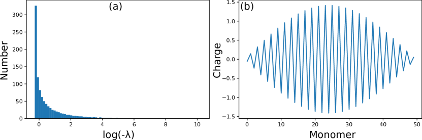
Figure S1: SCD value analysis. (a) The distribution of eigenvalues of the matrix ${\hat{B}}_{1000}$ introduced in the text of this Supporting Information for addressing the mathematical principles of negative SCD values for overall neutral sequences; all eigenvalues (denoted by $\lambda$) shown are negative, demonstrating definitively that the SCD value of any overall charge neutral sequence with equal or fewer than 1,001 residues is negative. The methodology can readily be extended to test longer sequences insofar as it is numerically feasible to determine the pertinent eigenvalues. (b) The charge distribution of a 50-residue, overall charge-neutral polyampholyte that produces the least-negative SCD value attained numerically using gradient descent method.

Our theoretical $K_{\rm D}$s are within an order of magnitude of those measured by ITC. They are practically identical at 350 mM [NaCl], but our theoretical $K_{\rm D}$ decreases only $\approx 3$ times at [NaCl] = 165 mM rather than the $\approx 20$ times for ITC ²⁴. Our theory also predicts weaker ProT$\alpha$ binding for the H1 C-terminal region than for full-length H1 (Fig. S1) as seen in smFRET experiment, but our predicted $\sim 1.5$ times increase in $K_{\rm D}$ is less than the $\approx 20$ times measured by smFRET experiment ²³. In general, our cluster expansion (Eq. S12), which is a high-$T$ expansion ⁴⁸, is less accurate when electrostatic interaction is strong, such as at zero or low salt, because $B_{2}$ in Eq. 12 includes only two terms in a perturbation series, neglecting attractive terms of order $l_{\rm B}^{3}$ and higher. This consideration offers a perspective to understand the modest difference between our theory and ITC measurement at low salt. However, although the partial agreement between theory and ITC is tantalizing, our current theory should be most useful for conceptual and semi-quantitative investigation of comparative sequence dependence of different IDP complexes rather than as a quantitative predictor for the absolute binding affinity of a particular pair of IDPs. Our theory ignores many structural and energetic details for tractability, including ion condensation, the effect of which has a salt dependence ^{51, 36} that might underlie the dramatic salt dependence of $K_{\rm D}$ as seen by smFRET ²³, and other solvation effects that might necessitate an effective separation-dependent dielectric ^{52, 53}. After all, explicit-chain simulation has produced a $K_{\rm D}\approx 7\times 10^{-9}$ $\mu$M which is $>300$ times more favorable than that measured by smFRET ²³, underscoring that, as it stands, all reported H1-ProT$\alpha$ experimental data are within theoretical possibilities.

Limitations of our analytical formulation notwithstanding, an important physical insight is gained by inspecting the contributions in Eq. 12 to the predicted H1-ProT$\alpha$ behavior from the first mean-field term that depends solely on overall net charges of the two IDPs and the second, sequence-specific term. Remarkably, the mean-field net-charge term alone yields $K_{\rm D}$s that are 30–40 times larger than those calculated using both terms in Eq. 12 (Table S1), indicating that the net-charge term is almost inconsequential and that the sequence-dependent term—and by extension also the $O(l_{\rm B}^{3})$ terms—embodying the dynamic disorder of IDP conformations play a dominant role in the favorable assembly of fuzzy IDP complexes.

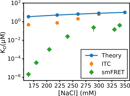
Figure 1: Theoretical and experimental H1-ProT$\alpha$ dissociation constants as functions of salt concentration. Data plotted are provided in Table S1 in the Supporting Information.

Assembly of binary fuzzy complex is highly sequence specific. We now proceed to compare the binding of different IDP pairs and analyze them systematically by expressing the $B_{2}$ for electrostatic interactions in Eq. 12 as

$$B_{2}\approx\frac{4\pi l_{\rm B}}{\kappa_{\rm D}^{2}}q^{A}q^{B}-4l_{\rm B}^{2}\int\frac{dkk^{2}}{(k^{2}+\kappa_{\rm D}^{2})^{2}}\tsum\slimits@_{s,t=1}^{N_{A}}\tsum\slimits@_{l,m=1}^{N_{B}}\sigma^{A}_{s}\sigma^{A}_{t}\sigma^{B}_{l}\sigma^{B}_{m}e^{-\frac{1}{6}(kb)^{2}[|s-t|+|l-m|]}\equiv F_{1}+F_{2}\;,$$ (15)

where $F_{1}$ is an $O(l_{\rm B})$ term arising from the interaction between the net charges $q^{A}$ of chain $A$ and $q^{B}$ of chain $B$, and $F_{2}$ accounts for sequence specificity. We further rewrite $F_{2}$ as

$$F_{2}= -4l_{\rm B}^{2}\int_{0}\frac{dkk^{2}}{(k^{2}+\kappa_{\rm D}^{2})^{2}}\tsum\slimits@_{s,t=1}^{N_{A}}\tsum\slimits@_{l,m=1}^{N_{B}}\sigma^{A}_{s}\sigma^{A}_{t}\sigma^{B}_{l}\sigma^{B}_{m}e^{-\frac{1}{6}(kb)^{2}(|s-t|+|l-m|)}$$ (16)

$$-\frac{4l_{\rm B}^{2}b}{\sqrt{6}}\tsum\slimits@_{s,t=1}^{N_{A}}\tsum\slimits@_{l,m=1}^{N_{B}}\sigma^{A}_{s}\sigma^{A}_{t}\sigma^{B}_{l}\sigma^{B}_{m}I_{(|s-t|+|l-m|)}\;,$$

where $I$ is the following integral over the variable $\bar{k}$:

$$I_{X}=\int_{0}\frac{d\bar{k}\bar{k}^{2}}{(\bar{k}^{2}+\bar{\kappa_{\rm D}}^{2})^{2}}e^{-X\bar{k}^{2}}$$ (17)

with $\bar{k}\equiv kb/\sqrt{6}$, $\bar{\kappa_{\rm D}}\equiv\kappa_{\rm D}b/\sqrt{6}$, and $X\equiv|s-t|+|l-m|$. Using integration by parts,

$$I_{X}=-\frac{1}{2}\int_{0}d\bar{k}(\bar{k}e^{-X\bar{k}^{2}})\frac{d}{d\bar{k}}\frac{1}{\bar{k}^{2}+\bar{\kappa_{\rm D}}^{2}}= -\frac{1}{2}\left.\frac{\bar{k}e^{-X\bar{k}^{2}}}{\bar{k}^{2}+\bar{\kappa_{\rm D}}^{2}}\right|_{0}+\frac{1}{2}\int_{0}d\bar{k}\frac{1-2X\bar{k}^{2}}{\bar{k}^{2}+\bar{\kappa_{\rm D}}^{2}}e^{-X\bar{k}^{2}}$$ (18)

$$= \left(\frac{1}{2}+X\bar{\kappa_{\rm D}}^{2}\right)\int_{0}d\bar{k}\frac{e^{-X\bar{k}^{2}}}{\bar{k}^{2}+\bar{\kappa_{\rm D}}^{2}}-X\int_{0}d\bar{k}e^{-X\bar{k}^{2}}$$

$$= \left(\frac{\pi}{4\bar{\kappa_{\rm D}}}+\frac{\pi X\bar{\kappa_{\rm D}}}{2}\right)e^{X\bar{\kappa_{\rm D}}^{2}}{\rm erfc}\left(\bar{\kappa_{\rm D}}\sqrt{X}\right)-\frac{\sqrt{\pi X}}{2}\;,$$

where ${\rm erfc}(z)=(2/\sqrt{\pi})\int_{z}dt\exp(-t^{2})$ is the complementary error function.⁵⁴ In a $\bar{\kappa_{\rm D}}\ll 1$ regime that allows for the substitution of ${\rm erfc}(z)$ and $e^{z^{2}}$ by their Taylor series,

$$e^{z^{2}}{\rm erfc}(z)=1-\frac{2z}{\sqrt{\pi}}+z^{2}+O(z^{3})\;,$$ (19)

setting $z=\sqrt{X}\bar{\kappa_{\rm D}}$ and applying Eq. 19 to the last expression in Eq. 18 yields

$$I_{X}=\frac{\pi}{4\bar{\kappa_{\rm D}}}-\sqrt{\pi X}+\frac{3}{4}\pi\bar{\kappa_{\rm D}}X+O(\bar{\kappa_{\rm D}}^{2})\;.$$ (20)

In that case $F_{2}$ in Eq. 15 becomes

$$F_{2}=-\frac{4l_{\rm B}^{2}b}{\sqrt{6}}\left[\frac{\pi\sqrt{6}}{4\kappa_{\rm D}b}\left(q^{A}\right)^{2}\left(q^{B}\right)^{2}-\sqrt{\pi}\tsum\slimits@_{s,t=1}^{N_{A}}\tsum\slimits@_{l,m=1}^{N_{B}}\sigma^{A}_{s}\sigma^{A}_{t}\sigma^{B}_{l}\sigma^{B}_{m}\sqrt{|s-t|+|l-m|}\right]+O(\bar{\kappa_{\rm D}})\;,$$ (21)

where the first term is an $O(l_{\rm B}^{2})$ contribution due to the chains’ net charges $q^{A}$ and $q^{B}$, the second term involving individual $\sigma^{i}_{s}$s then provides the lowest-order (in $\bar{\kappa_{\rm D}}$) account of sequence specificity. A two-chain sequence charge pattern parameter, which we refer to as “joint sequence charge decoration” (jSCD) because of its formal similarity with the single-chain SCD (Ref. 29), emerges naturally from this sequence-specific term in Eq. 21:

$$\text{jSCD}(\sigma^{A},\sigma^{B})\equiv-\frac{1}{2{N_{A}}{N_{B}}}\tsum\slimits@_{s,t=1}^{N_{A}}\tsum\slimits@_{l,m=1}^{N_{B}}\sigma^{A}_{s}\sigma^{A}_{t}\sigma^{B}_{l}\sigma^{B}_{m}\sqrt{|s-t|+|l-m|}.$$ (22)

When one or both of the chains are overall neutral, i.e., $q^{A}=0$ and/or $q^{B}=0$ ($q^{A}q^{B}=0$), both $F_{1}$ and the first term of $F_{2}$ in Eq. 21 vanish, leaving $B_{2}$ in a form that is is proportional to jSCD:

$$\left.B_{2}\right|_{\kappa_{\rm D}\to 0,q^{A}q^{B}=0}=-8\sqrt{\frac{\pi}{6}}l_{\rm B}^{2}b{N_{A}}{N_{B}}\times\text{jSCD}(\sigma^{A},\sigma^{B})\;.$$ (23)

When both chains are not overall neutral, i.e., $q^{A}\neq 0$ and $q^{B}\neq 0$ ($q^{A}q^{B}\neq 0$), the $q^{A}q^{B}$ terms in Eqs. 15 and 21 are part of the Taylor series of the Mayer $f$-function of the mean-field (MF) net charge interaction, as can be seen from the identity of these terms with the first two terms in the Taylor expansion of the second virial coefficient (denoted $B_{2}^{\rm MF}$ here) of two point charges interacting via a screened Coulomb potential:

$$B_{2}^{\rm MF}= \int d^{3}r\left(1-e^{-l_{\rm B}q^{A}q^{B}e^{-\kappa_{\rm D}r}/r}\right)$$ (24)

$$= 4\pi\int_{0}drr^{2}\left(l_{\rm B}\frac{q^{A}q^{B}e^{-\kappa_{\rm D}r}}{r}-\frac{l_{\rm B}^{2}}{2}\frac{\left(q^{A}\right)^{2}\left(q^{B}\right)^{2}e^{-2\kappa_{\rm D}r}}{r^{2}}+O(l_{\rm B}^{3})\right)$$

$$= \frac{4\pi l_{\rm B}q^{A}q^{B}}{\kappa_{\rm D}^{2}}-\frac{\pi l_{\rm B}^{2}}{\kappa_{\rm D}}\left(q^{A}\right)^{2}\left(q^{B}\right)^{2}+O(l_{\rm B}^{3})\;.$$

Since these $q^{A}q^{B}$ terms in Eqs. 15 and 21 do not involve individual $\sigma^{i}_{s}$s and thus include no sequence specificity, the jSCD term is always the lowest-order term (in $\bar{\kappa_{\rm D}}$) that takes into account sequence specificity for overall neutral as well as overall non-neutral chains. We also note that the divergence of these net charge terms in the $\kappa_{\rm D}\to 0$ limit is the well-recognized infrared divergence caused by the long-range nature of pure Coulomb interaction, which is regularized as long as there is nonzero screening ($\kappa_{\rm D}>0$).

We apply Eq. 23 to the set of 30 fully charged, overall neutral 50-monomer sv sequences introduced by Das and Pappu. Each of these sequences contains 25 positive ($+$) and 25 negative ($-$) charges but they have different charge patterns²⁸ as quantitied by $\kappa$ and SCD ³⁰ (Fig. 2a). Different binding constants ($K_{\rm D}^{-1}$) ranging widely from under 5 $\mu$M to over 2 mM are predicted by Eq. 23 for the 900 sv sequence pairs, exhibiting a general trend of increasing binding affinity with increasing charge segregation of the interacting IDPs as measured by SCD (Fig. 2b) and $\kappa$ (Fig. 3).

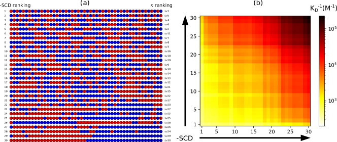
Figure 2: Fuzzy complex binding depends strongly on sequence charge patterns. (a) The 30 sv sequences (red: $-1$, blue: $+1$) ordered by their SCD values (left) whereas the number after the “sv” (right) indicates their ranking by $\kappa$ (Ref. 28). (b) Heatmap of binding affinities of all $30\times 30$ sv pairs. Sequences with higher $-$SCD values bind more tightly.

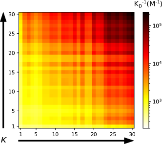
Figure 3: Heatmap of binding affinities of all 30 30 pairs of overall charge neutral sv sequences arranged in increasing value of the $\kappa$ parameter of Das and Pappu²⁸ along both axes. Consistent with the trend shown in Fig. 2b for SCD dependence, sequences with higher $\kappa$ values here are seen to have generally higher binding affinities.

New analytical relationship with phase separation. jSCD characterizes not only binary fuzzy IDP complexes but also IDP phase separation. In the random phase approximation (RPA) theory of phase separation ^{33, 35} of overall charge neutral sequences in the absence of salt and short-range cutoff of Coulomb interaction (Eqs. 39 and 40 of Ref. 35 with ${\tilde{k}}^{2}[1+{\tilde{k}}^{2}]\to{\tilde{k}}^{2}$), the electrostatic free energy $f_{\text{el}}$ may be expanded through $O(l_{\rm B}^{2})$ as

$$f_{\text{el}} =\int_{0}\frac{dkk^{2}}{4\pi^{2}}\left\{\ln\left[1+\frac{4\pi\phi_{m}}{k^{2}T^{*}N}\langle\sigma|\hat{G}_{\rm M}(k)|\sigma\rangle\right]-\frac{4\pi\phi_{m}}{k^{2}T^{*}N}\langle\sigma|\hat{G}_{\rm M}(k)|\sigma\rangle\right\}$$ (25)

$$=-\frac{2\phi_{m}^{2}}{T^{*2}N^{2}}\int_{0}\frac{dk}{k^{2}}\langle\sigma|\hat{G}_{\rm M}(k)|\sigma\rangle^{2}+O(l_{\rm B}^{3})$$

$$=-\frac{\phi_{m}^{2}}{T^{*2}}\sqrt{\frac{8\pi}{3}}\text{jSCD}(\sigma,\sigma)+O(l_{\rm B}^{3}),$$

where $N$ is chain length and $\phi_{m}$ is volume fraction of the IDP, $T^{*}\equiv b/l_{\rm B}$ is reduced temperature, and $\langle\sigma|\hat{G}_{\rm M}(k)|\sigma\rangle=\tsum\slimits@_{s,t=1}^{N}\sigma_{s}\sigma_{t}\exp(-k^{2}|s-t|/6)$ is the charge structure factor ($\tsum\slimits@_{s=1}^{N}\sigma_{s}=0$ for neutral sequences). The $\phi_{m}^{2}$ term in Eq. 25 allows for an approximate sequence-dependent Flory-Huggin (FH) theory of phase separation, which we term jSCD-FH, with an effective FH $\chi$ parameter

$$\chi(\sigma,\sigma)\equiv\sqrt{\frac{8\pi}{3}}\frac{\text{jSCD}(\sigma,\sigma)}{T^{*2}}\;.$$ (26)

For two IDP species $A,B$, one similarly obtains $\chi(\sigma^{A},\sigma^{B})=\sqrt{8\pi/3}[\text{jSCD}(\sigma^{A},\sigma^{B})]/T^{*2}$ and

$$f_{\text{el}}=-\chi(\sigma^{A},\sigma^{A})\phi_{A}^{2}-2\chi(\sigma^{A},\sigma^{B})\phi_{A}\phi_{B}-\chi(\sigma^{B},\sigma^{B})\phi_{B}^{2}+O(l_{\rm B}^{3})\;$$ (27)

in the form of the FH interaction terms for a-two-IDP species system (Eq. 27 of Ref. 16).

Recognizing $\chi=\chi_{\rm cr}=(\sqrt{N}+1)^{2}/(2N)$ at the FH critical temperature $T^{*}_{\rm cr}$, Eq. 26 suggests that for $N=50$,

$$T^{*}_{\rm cr}(\sigma)\approx 2.11\times\text{jSCD}^{1/2}(\sigma,\sigma)\;.$$ (28)

A strong correlation between jSCD and the product of its two component SCDs is suggested by Fig. 2b. Indeed, for the 30 sv sequences as well as 1,000 randomly generated overall charge neutral 50mer sequences (see Supporting Information for description), $\text{jSCD}(\sigma,\sigma)\approx 0.293\times|\text{SCD}(\sigma)|^{1.77}$ and $\text{jSCD}(\sigma^{A},\sigma^{B})\approx 0.313[\text{SCD}(\sigma^{A})\times\text{SCD}(\sigma^{B})]^{0.920}$ (Fig. 4a,b). The correlations are excellent aside from slightly more scatter around SCD${}^{2}\sim 1$. To assess the robustness of these correlations, we consider also a modified Coulomb potential $l_{\rm B}[1-\exp(-r/b)]/r$ with short-range cutoff used in RPA ^{55, 33, 35, 30, 16} to derive a modified jSCD,

$$\text{jSCD}_{\text{cutoff}}(\sigma^{A},\sigma^{B})\equiv\frac{1}{{N_{A}}{N_{B}}}\sqrt{\frac{3}{2\pi}}\int_{0}\frac{dk}{k^{2}(1+k^{2})^{2}}\tsum\slimits@_{s,t=1}^{N_{A}}\tsum\slimits@_{l,m=1}^{N_{B}}\sigma^{A}_{s}\sigma^{A}_{t}\sigma^{B}_{l}\sigma^{B}_{m}e^{-\frac{1}{6}(kb)^{2}[|s-t|+|l-m|]}\;,$$ (29)

and find that $\text{jSCD}_{\rm cutoff}(\sigma,\sigma)\approx 0.118\times|\text{SCD}(\sigma)|^{2.007}$ and $\text{jSCD}_{\rm cutoff}(\sigma^{A},\sigma^{B})\approx 0.109[\text{SCD}(\sigma^{A})\times\text{SCD}(\sigma^{B})]^{1.003}$ (Fig. 4c,d). Interestingly, combining the $\text{jSCD}_{\rm cutoff}(\sigma,\sigma)$ scaling and Eq. 28 rationalizes the $T^{*}_{\rm cr}\;\tilde{\propto}\;\text{SCD}$ scaling in Ref. 30 (Fig. 5); and this analytical result is in line with the relation between $B_{2}$ and $T^{*}_{\rm cr}$ deduced from explicit-chain simulations ⁴⁶. Taking into account also the $\text{jSCD}_{\rm cutoff}(\sigma^{A},\sigma^{B})$ scaling and Eq. 27 rationalizes the $\chi(\sigma^{A},\sigma^{B})=\sqrt{\chi(\sigma^{A},\sigma^{A})\;\chi(\sigma^{B},\sigma^{B})}$ relation in Ref. 16 (Fig. 6). Not unexpectedly, in both cases, approximate mean-field jSCD-FH produces a trend consistent with RPA, but entails a sharper dependence of phase behaviors on SCD than that predicted by RPA (Figs. 5 and 6). In this connection, it is instructive to note that the general trend of sequence dependent critical temperature of polyampholyte phase separation has recently been shown to agree largely with that obtained from field-theoretic simulations ⁵⁶, despite the RPA’s expected limitations in accounting for polyampholyte phase behaviors at very low concentrations.

Previously, the tendency of the populations of two polyampholytes $A$ and $B$ to demix upon phase separation (as quantified, e.g., by an ${\cal A}_{\alpha\beta}$ parameter) was reported to correlate with their SCD difference $\text{SCD}(\sigma^{B})-\text{SCD}(\sigma^{A})$ (Ref. 16 and Fig. 6d). In view of the above theoretical development and the fact that ${\cal A}_{\alpha\beta}$ $\text{SCD}(\sigma^{B})-\text{SCD}(\sigma^{A})$ was observed only for a set of six sv pairs ($A$ and $B$) all having sv28 as sequence $A$, this previously observed empirical correlation should now be viewed as a special case of an expected general correlation between $\text{jSCD}(\sigma^{A},\sigma^{B})$ and the tendency for demixing of sequences $A$ and $B$ upon phase separation because in the special case when $\text{SCD}(\sigma^{A})={\rm constant}$, $\text{jSCD}(\sigma^{A},\sigma^{B})$ $\tilde{\propto}$ $\text{SCD}(\sigma^{A})\times\text{SCD}(\sigma^{B})$ $\tilde{\propto}$ $[\text{SCD}(\sigma^{B})-\text{SCD}(\sigma^{A})]+{\rm constant}$.

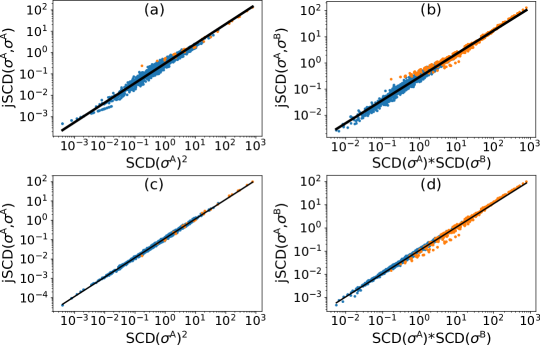
Figure 4: Correlation between single- and double-chain sequence charge pattern parameters. jSCD vs $\text{SCD}^{2}$ scatter plots for homotypic (a, c) or heterotypic (b, d) pairs among the $30\times 30$ pairs of sv sequences (orange) and 1,000 random pairs of partially-charged, overall neutral 50mers (blue) interacting via a pure Coulomb potential (a, b) or a Coulomb potential with a short-range cutoff (c, d). Black lines are power-law regressions; square of Pearson coefficient $r^{2}=$ (a) 0.983, (b) 0.967, (c) 0.997, and (d) 0.994. The correlation is good for both jSCD and jSCD_cutoff but their fitted scaling exponents are not identical. Apparently, SCD $<0$ for all overall charge neutral sequences (see discussion in Supporting Information and Fig. S1).

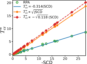
Figure 5: Approximate mean-field jSCD-FH phase separation theories entail stronger dependence of critical temperature $T^{*}_{\rm cr}$ on SCD than that predicted by RPA theory. Results shown are for the 30 sv sequences of Das and Pappu ²⁸. Critical temperatures calculated using RPA (green symbols) and its linear fit $T^{*}_{\rm cr}=-0.314\times\text{SCD}$ (blue line) are taken from Fig. 3b of Ref. 30. $T^{*}_{\rm cr}$ values computed here based on the jSCD-FH result in Eq. 28 and the jSCD_cutoff expression in Eq. 29, i.e., $T^{*}_{\rm cr}=2.11\sqrt{\text{jSCD}_{\rm cutoff}}$, are plotted in orange. The linear fit to the data points is provided in the same color. Slightly different jSCD-FH $T^{*}_{\rm cr}$ values are obtained using the formula $T^{*}_{\rm cr}=-2.11\sqrt{0.118}\times\text{SCD}$ solely by replacing the actual $\text{jSCD}_{\rm cutoff}$ values with the fitted value $\text{jSCD}_{\rm cutoff}=0.118\times(\text{SCD})^{2}$ deduced from Fig. 4c. Data in this plot indicate that both of the two jSCD-FH formulations capture the $T^{*}_{\rm cr}\;\tilde{\propto}\;\text{SCD}$ relation ³⁰ very well but overestimate the phase separation propensities relative to the RPA-predicted propensities for all 30 sv sequences.

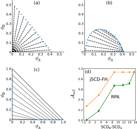
Figure 6: Binary phase diagrams generated by the approximate jSCD-based effective Flory-Huggins (jSCD-FH) interaction free energy given by Eq. 27 with the $\chi$ parameters given by Eq. 26 with $T^{*}=10$. Sequence $A$ is sv28 and sequence $B$s are (a) sv24, (b) sv25, and (c) sv20. $\phi$s are volume fractions of the polyampholytes. Blue dots are numerically solved phase-separated states $\alpha\equiv(\phi_{A}^{\alpha},\phi_{B}^{\alpha})$ and $\beta\equiv(\phi_{A}^{\beta},\phi_{B}^{\beta})$ [the $\beta$ here for labeling phase-separated states is not to be confused with the reciprocal Boltzmann factor $1/k_{\rm B}T$]; black dashed lines are tie lines connecting an $\alpha$–$\beta$ pair of coexisting states. Consistent with the RPA phase diagrams provided in Fig. 3 of Ref. 16, panels (a)–(c) here of jSCD-FH results show the same general trend that sequences with similar SCDs coalesce whereas those with significantly different SCDs exclude each other; but the degree of exclusion predicted by the present jSCD-FH theory is significantly higher than that predicted previously by RPA theory. (d) Variation of the composition asymmetry measure, ${\cal A}_{\alpha\beta}$, which is a demixing parameter (vertical axis), with the difference in SCD values of the sequence pair (horizontal axis; $\text{SCD}_{A}=\text{SCD}(\sigma^{A})$, $\text{SCD}_{B}=\text{SCD}(\sigma^{B})$). The measure ${\cal A}_{\alpha\beta}\equiv(2/\pi)\langle|\tan^{-1}(\phi_{A}^{\alpha}/\phi_{B}^{\alpha})-\tan^{-1}(\phi_{A}^{\beta}/\phi_{B}^{\beta})|\rangle$, where the $\langle\@cdots\rangle$ average is over all tie-line connected $\alpha$–$\beta$ pairs, is defined in Eq. 26 of Ref. 16 to quantify the tendency of two sequences $A$ and $B$ in a solution system to demix upon separation into two phases $\alpha$ and $\beta$. The orange jSCD-FH data points here are seen to be always higher than the corresponding green RPA data points, indicating that the more approximate mean-field jSCD-FH formulation always overestimates demixing propensity. Lines joining data points are guides for the eye. The last three jSCD-FH data points are connected by dashed lines instead of solid lines to underscore the fact that ${\cal A}_{\alpha\beta}$ is already saturated at the third (sv28–sv20) sequence pairs shown and the remaining ${\cal A}_{\alpha\beta}$ data points for larger SCD_B $-$ SCD_A differences remain at the same saturated value.

Theory-predicted trend is consistent with simulations and Kuhn length renormalization. We now assess our approximate theory by comparing its predictions with coarse-grained molecular dynamics simulations ³⁸ of six sv sequence pairs. Details of the explicit-chain model is in the Supporting Information. Because bound IDPs in a fuzzy complex are dynamic, their configurations are diverse. The IDP chains in some bound configurations are relatively open, some are highly intertwined, others can take the form of two relatively compact chains interacting favorably mostly via residues situated on the surface of their individually compact conformations (Fig. 7a). Taking into account this diversity, we sample all intermolecular residue-residue distances between the model IDPs (rather than merely their center-of-mass distances) and use the appearance of a bimodal distribution to define binding (Fig. 7b) with binding probability $\theta$ given by the fractional area covered by the small-distance peak. To better quantify the role of favorable interchain interaction—rather than random collision—in the formation of IDP complexes, we subtract a reference probability, $4\pi r_{\rm cut}^{3}/(3V)$, that two particles in a simulation box of size $V$ will be within the cutoff distance $r_{\rm cut}$ that defines the the small-distance peak in Fig. 7b; and compare $\tilde{\theta}\equiv\theta-4\pi r_{\rm cut}^{3}/(3V)$ with theoretical predictions.

For the sequence pairs considered, theoretical $K_{\rm D}^{-1}$ is generally substantially higher than simulated $K_{\rm D}^{-1}$ at the same temperature. The mismatch likely arises from differences in the two models; for example, excluded volume is considered in the simulation but not in the present analytical theory. For the same reason, a similar mismatch between theory and explicit-chain simulation has been noted in the study of phase separation of sv aequences ^{30, 38}. Nonetheless, sequence-dependent trends of binding predicted by theory and simulation are largely similar (Fig. 7c). Notably, both theory and simulation posit that sv24–sv28 binds more strongly than sv25–sv28, exhibiting a rank order that is consistent with SCD (sv24 has a larger $-$SCD value than sv25) but not $\kappa$ (sv24 has a smaller $\kappa$ parameter than sv25).

However, theory and simulation disagree on the rank order of sv15–sv28 and sv20–sv28 binding affinities (Fig. 7c). As a first step in addressing this discrepancy, we examine more closely the impact of using a Gaussian-chain assumption to derive the $B_{2}$ formula in Eq. 12.

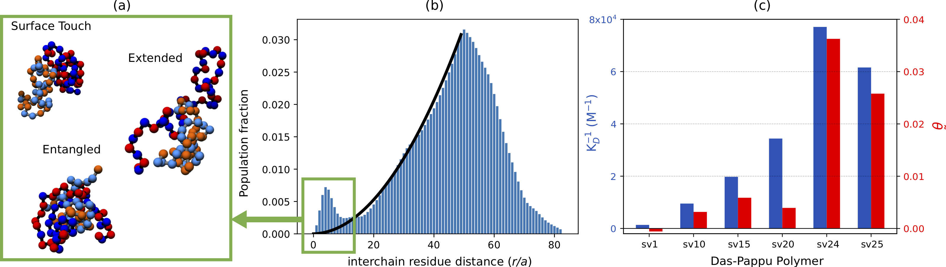
Figure 7: Comparing analytical theory against explicit-chain simulation. Results from simulations are for $T^{*}=0.35$. (a) Snapshots of fuzzy complexes of sv28 (cyan/orange: $+/-$) with different partners (blue/red: $+/-$): sv24 (surface touch), s25 (entangled) and sv1 (extended). (b) Distribution (histogram) of sv24–sv28 interchain residue-residue distance among 1,000,000 snapshots. The small-$r$ peak region (marked by the green frame) is the bound state. The black curve is the baseline distribution of distance between a pair of non-interacting particles in the same simulation box. (c) Theoretical $K_{\rm D}$ (blue) vs simulated $\tilde{\theta}$ (red), of sv28 with various partners (horizontal axis), where $\tilde{\theta}\equiv\theta-\theta_{0}$ with $\theta_{0}=4\pi\times 10^{3}/(3\times 100^{3})$ being the baseline probability that two non-interacting particles is $<10a$ apart. The $\tilde{\theta}<0$ result for sv1 means that the net interaction between sv28 and sv1 is repulsive in the simulation.

The Gaussian-chain approximation in the general formula for $B_{2}$ in Eq. 8 is for tractability. But in reality intrachain residue-residue correlation is physically affected by intrachain Coulomb interaction, as illustrated by the simulation snapshots in Fig. 7a. Several analytical approaches have been proposed to account for this effect approximately, including that of Sawle and Ghosh for polyampholytes ²⁹ and that of Shen and Wang for polyelectrolytes ⁵⁷. Here we focus on the method in Ref. 29, which entails deriving sequence-dependent effective, or renormalized, Kuhn lengths, denoted as $x^{i}_{st}b$ for residue pair $s,t$ in chain $i$, to replace the “bare” Kuhn length $b$ in the original simple Gaussian formulation. In other words, the modification

$$\left[\hat{P}^{i}({\bf k})\right]_{st}\approx\exp\left[-\frac{(kb)^{2}}{6}|s-t|\right]\to\exp\left[-\frac{(kb)^{2}}{6}x^{i}_{st}|s-t|\right]\;$$ (30)

is applied to Eq. 10. In this approach, instead of assuming that the conformational distribution of each of the two IDP chains in our binary interacting IDP-IDP system is that of a simple Gaussian chain as if it experiences no interaction other than the contraints of chain connectivity, the impact of the intrachain part of the interaction in the system on the conformational distribution of an individual IDP chain is taken into account approximately by treating the IDP as a modified Gaussian chain with a renormalized Kuhn length ²⁹. As such, it should be noted that this renormalization procedure is performed on a single isolated chain without addressing effects of interchain interactions.

Recognizing that the simple Gaussian-chain correlation function in Eq. 10 is a consequence of a single-chain Hamiltonian ${\cal H}^{i}_{0}[{\bf R}^{i}]$ containing only terms for elastic chain connectivity, viz.,

$${\cal H}^{i}_{0}[{\bf R}^{i}]=\frac{3}{2b^{2}}\tsum\slimits@_{s=1}^{N_{i}-1}\left|{\bf R}^{i}_{s+1}-{\bf R}^{i}_{s}\right|^{2}\;,$$ (31)

we now also take into consideration an intrachain interaction potential $\,{\cal U}^{i}[{\bf R}^{i}]$ that includes electrostatic interaction and excluded-volume repulsion,

$$\,{\cal U}^{i}[{\bf R}^{i}]=\tsum\slimits@_{s>t=1}^{N_{i}}\left[l_{\rm B}\sigma^{i}_{s}\sigma^{i}_{t}\frac{e^{-\kappa_{\rm D}|{\bf R}^{i}_{s}-{\bf R}^{i}_{t}|}}{|{\bf R}^{i}_{s}-{\bf R}^{i}_{t}|}+w^{i}\delta^{3}({\bf R}^{i}_{s}-{\bf R}^{i}_{t})\right]\;,$$ (32)

where $w^{i}$ is the two-body excluded-volume repulsion strength for chain $i$. For the 30 sv sequences ²⁸ used in the present analysis, the $w^{i}$ values obtained from matching theory with result from explicit-chain atomic simulation conducted in the “intrinsic solvation” limit in the absence of electrostatic interactions²⁸ are available from Table 1 of Sawle and Ghosh ²⁹. A full Hamiltonian ${\cal H}^{i}$ is then given by the sum of Eqs. 31 and 32:

$${\cal H}^{i}[{\bf R}^{i}]={\cal H}^{i}_{0}[{\bf R}^{i}]+\,{\cal U}^{i}[{\bf R}^{i}]\;.$$ (33)

We assume, as in Ref. 29, that the full Hamiltonian can be approximated as the Hamiltonian ${\cal T}_{x}^{i}[{\bf R}^{i}]$ for a modified Gaussian chain with an effective Kuhn length $x^{i}b$, which is equivalent to $N_{i}b^{2}\rightarrow N_{i}b(x^{i}b)$ while holding the total contour length $N_{i}b$ unchanged (cf. Eqs. 1 and 2 of Ref. 29). In other words ⁴⁷,

$${\cal H}^{i}[{\bf R}^{i}]\approx{\cal T}_{x}^{i}[{\bf R}^{i}]\equiv\frac{3}{2xb^{2}}\tsum\slimits@_{s=1}^{N_{i}-1}\left|{\bf R}^{i}_{s+1}-{\bf R}^{i}_{s}\right|^{2}\;,$$ (34)

where $x$ is to be determined by the variational approach described in Ref. 29. Here we briefly summarize the concept and result, and refer the readers to the original paper²⁹ for methodological details. The approach consists of expressing the full Hamiltonian as a sum of the “principal” ${\cal T}_{x}^{i}$ component and a “perturbative” $\Delta{\cal H}^{i}_{x}$ term:

$${\cal H}^{i}[{\bf R}^{i}]={\cal T}_{x}^{i}[{\bf R}^{i}]+\Delta{\cal H}^{i}_{x}[{\bf R}^{i}],$$ (35)

where, by Eqs. 31, 32 and 34,

$$\Delta{\cal H}^{i}_{x}[{\bf R}^{i}]=\frac{3}{2b^{2}}\left(1-\frac{1}{x}\right)\tsum\slimits@_{s=1}^{N_{i}-1}\left|{\bf R}^{i}_{s+1}-{\bf R}^{i}_{s}\right|^{2}+\tsum\slimits@_{s>t=1}^{N_{i}}\left[l_{\rm B}\sigma^{i}_{s}\sigma^{i}_{t}\frac{e^{-\kappa_{\rm D}|{\bf R}^{i}_{s}-{\bf R}^{i}_{t}|}}{|{\bf R}^{i}_{s}-{\bf R}^{i}_{t}|}+w^{i}\delta^{3}({\bf R}^{i}_{s}-{\bf R}^{i}_{t})\right]\;.$$ (36)

Making use of the form in Eq. 34, the full thermodynamic average $\left\langle A\right\rangle$—Boltzmann-weighted by the full Hamiltonian ${\cal H}^{i}$—of any physical observable $A$ can be cast as an expansion in the power of the perturbative Hamiltonian $\Delta{\cal H}^{i}_{x}$ (Eq. 3 of Ref. 29):

$$\left\langle A\right\rangle=\left\langle A\right\rangle_{x}+\left\langle A\right\rangle_{x}\left\langle\Delta{\cal H}^{i}_{x}\right\rangle_{x}-\left\langle A\Delta{\cal H}^{i}_{x}\right\rangle_{x}+O\left[(\Delta{\cal H}^{i}_{x})^{2}\right]\;,$$ (37)

where the averages $\left\langle\@cdots\right\rangle$ and $\left\langle\@cdots\right\rangle_{x}$ are defined by

$$\left\langle A\right\rangle\equiv \;\frac{\int\mathscr{D}[{\bf R}^{i}]A[{\bf R}^{i}]e^{-{\cal H}^{i}[{\bf R}^{i}]}}{\int\mathscr{D}[{\bf R}^{i}]e^{-{\cal H}^{i}[{\bf R}^{i}]}}\;,$$ (38a)

$$\left\langle A\right\rangle_{x}\equiv \;\frac{\int\mathscr{D}[{\bf R}^{i}]A[{\bf R}^{i}]e^{-{\cal T}^{i}_{x}[{\bf R}^{i}]}}{\int\mathscr{D}[{\bf R}^{i}]e^{-{\cal T}^{i}_{x}[{\bf R}^{i}]}}\;.$$ (38b)

For any observable $A$ of interest, an optimal $x$ in this formalism is obtained by minimizing the difference between the averages weighted by the full ${\cal H}^{i}$ and the approximate ${\cal T}^{i}_{x}$ through eliminating the $O(\Delta{\cal H}^{i}_{x})$ term in Eq. 37. Imposing this condition allows us to solve for an optimal set of $x^{i}_{st}$ for a given $A$. Comparisons by Ghosh and coworkers of results from this theoretical approach against those from explicit-chain simulations have demonstrated that this is a rather accurate and effective method ^{29, 58}. Ideally, the correlation functions $\left[\hat{P}^{i}({\bf k})\right]_{st}$ themselves should be used as observables for the optimization; but that leads to insurmountable technical difficulties. Thus, following Ref. 29 (Eq. 11 of this reference), we use $|{\bf R}^{i}_{s}-{\bf R}^{i}_{t}|^{2}$ as observables to optimize $x^{i}_{st}$s. Accordingly, for each residue pair $s^{i},t^{i}$ on chain $i$, an optimized $x$ factor, $x^{i}_{st}$, is obtained by solving the equation

$$\left\langle|{\bf R}^{i}_{s}-{\bf R}^{i}_{t}|^{2}\right\rangle_{x^{i}_{st}}\left\langle\Delta{\cal H}^{i}_{x^{i}_{st}}\right\rangle_{x^{i}_{st}}=\left\langle|{\bf R}^{i}_{s}-{\bf R}^{i}_{t}|^{2}\Delta{\cal H}^{i}_{x^{i}_{st}}\right\rangle_{x^{i}_{st}}\;$$ (39)

using the formalism developed in Eqs. 6–10 of Ref. 29. These solved $x^{i}_{st}$ values are then used to rescale the two terms of the $X$ factor introduced in Eq. 17 to arrive at the expression

$$B_{2}=\frac{4\pi l_{\rm B}}{\kappa_{\rm D}^{2}}q^{A}q^{B}-4l_{\rm B}^{2}\int\frac{dkk^{2}}{(k^{2}+\kappa_{\rm D}^{2})^{2}}\tsum\slimits@_{s,t=1}^{N_{A}}\tsum\slimits@_{l,m=1}^{N_{B}}\sigma^{A}_{s}\sigma^{A}_{t}\sigma^{B}_{l}\sigma^{B}_{m}e^{-\frac{1}{6}(kb)^{2}[x^{A}_{st}|s-t|+x^{B}_{lm}|l-m|]}$$ (40)

for the second virial coefficient in the formulation with renormalized Kuhn lengths. In the case of a salt-free solution of overall charge neutral polymers, this expression reduces to

$$\left.B_{2}^{\rm eff}\right|_{\kappa_{\rm D}\to 0,q^{A}q^{B}=0}=4\sqrt{\frac{\pi}{6}}l_{\rm B}^{2}b\tsum\slimits@_{s,t=1}^{N_{A}}\tsum\slimits@_{l,m=1}^{N_{B}}\sigma^{A}_{s}\sigma^{A}_{t}\sigma^{B}_{l}\sigma^{B}_{m}\sqrt{x^{A}_{st}|s-t|+x^{B}_{lm}|l-m|}\;,$$ (41)

which is the modified (renormalized) form of Eq. 23.

The resulting heatmap of the $K_{\rm D}$ values calculated in this manner is provided in Fig. 8a. Unlike the results obtained using the base theory with a simple Gaussian chain model (Fig. 2b), the theory of renormalized Kuhn lengths predicts that some sv sequence pairs do not bind at all, as indicated by the white regions in Fig. 8a. Furthermore, instead of binding propensity being monotonic with charge segregation (quantified by $-$SCD) as predicted by the base theory, some sv sequence pairs deviate from the trend. Specifically, highly charge segregated sequences with large $-$SCD values seem to avoid interactions with sequences with only a medium charge segregation with moderate $-$SCD values.

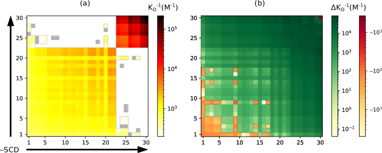
Figure 8: Heatmap of binding affinities of the $30\times 30$ overall charge neutral sv sequence pairs computed using Eq. 41 in the formulation with renormalized Kuhn lengths ²⁹. White squares indicate an unfavorable (repulsive) interaction and grey squares indicate a weak $K_{\rm D}$ of greater than 5 mM. The results are quite different from those provided in Fig. 2b for the base theory with a bare (not renormalized) Kuhn length. (b) Heatmap of difference in the same sequence pairs’ binding affinities predicted by the two theories (base-theory prediction minus renormalized-Kuhn-lengths prediction). In general, more charge segregated sequences, i.e., those with higher $-$SCD values, exhibit a higher reduction in binding affinities when intrachain interactions are accounted for approximately using renormalized Kuhn lengths.

These contrasts between the base theory and the formulation with renormalized Kuhn lengths are underscored in Fig. 8b where the numerical differences in predicted binding affinities by the two formulations are plotted. Apparently, the approximate account of intrachain interactions afforded by renormalized Kuhn lengths posits a larger decrease in binding affinities relative to that predicted by the base theory or high $-$SCD sequences than for low $-$SCD sequences. The $K_{\rm D}$s predicted by the two theories and the binding probabilities obtained from explicit-chain simulations for several example sv sequence pairs are compared in more detail in Fig. 9. These predictions are physically intuitive as sequences with larger $-$SCDs generally have stronger intrachain interactions, although the magnitude of the effect is likely overestimated. With the last caveat, the higher simulated binding of sv15–sv28 relative to that of sv20–sv28 may be understood in terms of sv20’s more favorable intrachain interaction (Fig. 9). In this context, it would be extremely interesting to explore in future investigations the impact of the improved formulation of $x^{A}_{st}$ and $x^{B}_{lm}$ proposed recently by Huihui and Ghosh ⁵⁸ on the association of sv model sequences and other polyampholytes. In particular, for the polyelectrolyte H1-ProT$\alpha$ system considered above (Fig. 1), since the highly open individual H1 and ProT$\alpha$ conformations at low salt are expected to entail more favorable H1-ProT$\alpha$ interactions than their less open individual conformations at high salt, an analytical theory with renormalized Kuhn lengths for individual IDP chains would likely lead to a higher salt sensitivity for $K_{\rm D}$ and hence better agreement with experiments. This expectation, however, remains to be tested.

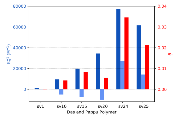
Figure 9: Binding affinities of example sv sequence pairs. Theoretical and simulation results are provided for sv28 pairing individually with sv1, sv10, sv15, sv20, sv24, and sv25. As in Fig. 7, predictions by theory using simple Gaussian chains without renormalized Kuhn lengths (Eq. 23) are shown in dark blue, explicit-chain simulation results, calculated anew here using the regression method described in the Supporting Information for $T^{*}=0.35$ (Eq. S29 and Table S2), are shown in red. Included here for comparison are predictions by theory using renormalized Kuhn lengths, shown in light blue, as prescribed by Eq. 41. It is noteworthy from this comparison that effects of intrachain interactions on single-chain conformational distribution may afford a partial rationalization for the discrepancy between simple theory (dark blue) and explicit-chain simulation (red) for sv20–sv28 binding but for the present case such effects are likely overestimated by the method of renormalized Kuhn lengths²⁹ to result in a net repulsion (negative light blue bars for not only sv20–sv28 but also sv10–sv28 and sv15–sv28).

4 Conclusions

In summary, we have developed an analytical account of charge sequence-dependent fuzzy binary complexes with novel two-chain charge pattern parameter jSCD emerging as a key determinant not only of binary binding affinity but also of multiple-chain phase separation. The formulation elucidates the dominant role of conformational disorder and sequence-specificity in IDP-IDP binding, and provides a footing for empirical correlation between single- and two-chain IDP properties with their sequence-dependent phase-separation propensities ^{30, 59, 46, 60, 61}. While the formulation is limited inasmuch as it is a high-temperature approximation and further developments, including extension to sequence patterns of uncharged residues ^{34, 26, 40, 31}, are desirable, the charge sequence dependence predicted herein is largely in line with explicit-chain simulation. As such, the present formalism offers conceptual advances as well as utility for experimental design and efficient screening of candidates of fuzzy complexes.

5 Acknowledgements

We thank Robert Best, Aritra Chowdhury, Julie Forman-Kay, Alex Holehouse, Jeetain Mittal, Rohit Pappu, and Wenwei Zheng for helpful discussions, and Ben Schuler for insightful comments on an earlier version of this paper (arXiv:1910.11194v1) and sharing unpublished data. This work was supported by Canadian Institutes of Health Research grants MOP-84281, NJT-155930, Natural Sciences and Engineering Research Council of Canada Discovery grant RGPIN-2018-04351, and computational resources provided by Compute/Calcul Canada.

The authors declare no conflict of interest.

Analytical Theory for Sequence-Specific Binary Fuzzy Complexes of Charged Intrinsically Disordered Proteins Alan N. Amin Contributed equally to this work Present address: Systems, Synthetic, and Quantitative Biology Program,
Harvard Medical School, Boston, Massachusetts, U.S.A. ^,§ Yi-Hsuan Lin Molecular Medicine, Hospital for Sick Children, Toronto, Ontario, Canada Contributed equally to this work Suman Das Hue Sun Chan Department of Molecular Genetics, University of Toronto, Toronto, Ontario, Canada

Supporting Information

6 Derivation for $B_{2}$ representations

Starting from the partition function representation (first equality of Eq. 3 in the main text),

$$B_{2}=V-\frac{{{\cal Q}_{A\!B}}}{{{\cal Q}_{A}}{{\cal Q}_{B}}}\;,$$

we denote the isolated single-chain Hamiltonians in units of $k_{\rm B}T$ ($k_{\rm B}$ is Boltzmann constant and $T$ is absolute temperature) for $A$ and $B$, respectively, as ${\cal H}^{A}[{\bf R}^{A}]$ and ${\cal H}^{B}[{\bf R}^{B}]$. The corresponding conformational partition functions are then given by

$${\cal Q}_{i}= \frac{1}{V}\int\mathscr{D}[{\bf R}^{i}]e^{-{\cal H}^{i}[{\bf R}^{i}]}\;,\;i=A,B$$ (S1a)

$${{\cal Q}_{A\!B}}= \frac{1}{V}\int\mathscr{D}[{\bf R}^{A}]\mathscr{D}[{\bf R}^{B}]e^{-{\cal H}^{A}[{\bf R}^{A}]-{\cal H}^{B}[{\bf R}^{B}]-\,{\cal U}^{AB}[{\bf R}^{A},{\bf R}^{B}]}\;,$$ (S1b)

where $1/V$ cancels the degeneracy due to translational invariance. It follows that

$$\frac{{{\cal Q}_{A\!B}}}{{{\cal Q}_{A}}{{\cal Q}_{B}}}= V\frac{\int\mathscr{D}[{\bf R}^{A}]\mathscr{D}[{\bf R}^{B}]e^{-{\cal H}^{A}[{\bf R}^{A}]-{\cal H}^{B}[{\bf R}^{B}]-\,{\cal U}^{AB}[{\bf R}^{A},{\bf R}^{B}]}}{\int\mathscr{D}[{\bf R}^{A}]e^{-{\cal H}^{A}[{\bf R}^{A}]}\int\mathscr{D}[{\bf R}^{B}]e^{-{\cal H}^{B}[{\bf R}^{B}]}}$$ (S2)

$$= V\int\mathscr{D}[{\bf R}^{A}]\mathscr{D}[{\bf R}^{B}]\frac{e^{-{\cal H}^{A}[{\bf R}^{A}]}}{\int\mathscr{D}[{\bf R}^{A}]e^{-{\cal H}^{A}[{\bf R}^{A}]}}\frac{e^{-{\cal H}^{B}[{\bf R}^{B}]}}{\int\mathscr{D}[{\bf R}^{B}]e^{-{\cal H}^{B}[{\bf R}^{B}]}}e^{-\,{\cal U}^{AB}[{\bf R}^{A},{\bf R}^{B}]}$$

$$V\int\mathscr{D}[{\bf R}^{A}]\mathscr{D}[{\bf R}^{B}]{\cal P}^{A}[{\bf R}^{A}]{\cal P}^{B}[{\bf R}^{B}]e^{-\,{\cal U}^{AB}[{\bf R}^{A},{\bf R}^{B}]}\;,$$

where, as noted in the main text, $\,{\cal U}^{AB}$ is in units of $k_{\rm B}T$, the single-chain probability density function

$${\cal P}^{i}[{\bf R}^{i}]\equiv\frac{e^{-{\cal H}^{i}[{\bf R}^{i}]}}{\int\mathscr{D}[{\bf R}^{i}]e^{-{\cal H}^{i}[{\bf R}^{i}]}}\;,\;i=A,B\;,$$ (S3)

and hence $\int\mathscr{D}[{\bf R}^{i}]{\cal P}^{i}[{\bf R}^{i}]=1$. Substituting Eq. S2 for ${{\cal Q}_{A\!B}}/({{\cal Q}_{A}}{{\cal Q}_{B}})$ results in the second equality in Eq. 3 of the main text, viz.,

$$B_{2}=V\int\mathscr{D}[{\bf R}^{A}]\mathscr{D}[{\bf R}^{B}]{\cal P}^{A}[{\bf R}^{A}]{\cal P}^{B}[{\bf R}^{B}]\left(1-e^{-\,{\cal U}^{AB}[{\bf R}^{A},{\bf R}^{B}]}\right)\;.$$

We now proceed to decouple translational invariance from the internal degrees of freedom of the chain molecules by the following change of coordinates:

$$\{{\bf R}^{i}_{1},{\bf R}^{i}_{2},\dots,{\bf R}^{i}_{N_{i}}\}\to\{{\bf R}^{i}_{1},\text{\bf\Large r}\,^{i}_{1},\text{\bf\Large r}\,^{i}_{2},\dots,\text{\bf\Large r}\,^{i}_{N_{i}-1}\},\;\text{\bf\Large r}\,^{i}_{s}\equiv{\bf R}^{i}_{s+1}-{\bf R}^{i}_{s}\;,$$ (S4)

which allows all intramolecular residue-residue distances of chain $i$ be expressed solely in terms of $\text{\bf\Large r}\,^{i}$s:

$${\bf R}^{i}_{s}-{\bf R}^{i}_{t}=\tsum\slimits@_{\tau=t}^{s-1}\text{\bf\Large r}\,^{i}_{\tau}\quad(s>t)\;.$$ (S5)

Since the potential energy of an isolated chain molecule in homogeneous space should depend only on the relative positions of its residues irrespective of the location of the chain’s center-of-mass, the single-chain Hamiltonian for chain $i$ should be a function of $\text{\bf\Large r}\,^{i}$s and independent of the position of any one single residue, which we may choose, without loss of generality, as the position ${\bf R}^{i}_{1}$ of the first residue. With this consideration, the partition functions ${{\cal Q}_{A}}$, ${{\cal Q}_{B}}$ can be rewritten as

$${\cal Q}_{i}=\frac{1}{V}\int d{\bf R}^{i}_{1}\mathscr{D}[\text{\bf\Large r}\,^{i}]e^{-{\cal H}^{i}[\text{\bf\Large r}\,^{i}]}=\int\mathscr{D}[\text{\bf\Large r}\,^{i}]e^{-{\cal H}^{i}[\text{\bf\Large r}\,^{i}]}\;,\quad i=A,B,$$ (S6)

where $\mathscr{D}[\text{\bf\Large r}\,^{i}]\equiv\tprod\slimits@_{s=1}^{N_{i}-1}d\text{\bf\Large r}\,^{i}_{s}$ and because $\int d{\bf R}^{i}_{1}/V=1$. For distances between residues on different chains,

$${\bf R}^{AB}_{st}\equiv{\bf R}^{A}_{s}-{\bf R}^{B}_{t}=\tsum\slimits@_{\tau=1}^{s}\text{\bf\Large r}\,^{A}_{\tau}-\tsum\slimits@_{\mu=1}^{t}\text{\bf\Large r}\,^{B}_{\mu}+{\bf R}^{AB}_{11}\;,$$ (S7)

where ${\bf R}^{AB}_{11}\equiv{\bf R}^{A}_{1}-{\bf R}^{B}_{1}$. Thus, the intermolecular interaction $\,{\cal U}^{AB}$ is a function of ${\bf R}^{AB}_{11}$ and $\text{\bf\Large r}\,^{A}$, $\text{\bf\Large r}\,^{B}$ (shorthand for $\{\text{\bf\Large r}\,^{A}\}=\{\text{\bf\Large r}\,^{A}_{1},\text{\bf\Large r}\,^{A}_{2},\dots,\text{\bf\Large r}\,^{i}_{N_{A}-1}\}$, $\{\text{\bf\Large r}\,^{B}\}=\{\text{\bf\Large r}\,^{B}_{1},\text{\bf\Large r}\,^{B}_{2},\dots,\text{\bf\Large r}\,^{i}_{N_{B}-1}\}$). The partition function of the $A$-$B$ complex may then be expressed as

$${{\cal Q}_{A\!B}}= \frac{1}{V}\int d{\bf R}^{A}_{1}d{\bf R}^{B}_{1}\mathscr{D}[\text{\bf\Large r}\,^{A}]\mathscr{D}[\text{\bf\Large r}\,^{B}]e^{-{\cal H}^{A}[\text{\bf\Large r}\,^{A}]-{\cal H}^{B}[\text{\bf\Large r}\,^{B}]-\,{\cal U}^{AB}[\text{\bf\Large r}\,^{A},\text{\bf\Large r}\,^{B},{\bf R}^{AB}_{11}]}$$ (S8)

$$= \int d{\bf R}^{AB}_{11}\mathscr{D}[\text{\bf\Large r}\,^{A}]\mathscr{D}[\text{\bf\Large r}\,^{B}]e^{-{\cal H}^{A}[\text{\bf\Large r}\,^{A}]-{\cal H}^{B}[\text{\bf\Large r}\,^{B}]-\,{\cal U}^{AB}[\text{\bf\Large r}\,^{A},\text{\bf\Large r}\,^{B},{\bf R}^{AB}_{11}]}\;,$$

where the second equality follows from the change of variable $\{{\bf R}^{A}_{1},{\bf R}^{B}_{1}\}\to\{{\bf R}^{AB}_{11},{\bf R}^{B}_{1}\}$ (Jacobian equals unity) and the fact that $\int d{\bf R}^{B}_{1}/V=1$. In terms of $\{\text{\bf\Large r}\,^{i}\}$, the single-chain conformational probability density functions are given by

$${\cal P}^{i}[\text{\bf\Large r}\,^{i}]=\frac{e^{-{\cal H}^{i}[\text{\bf\Large r}\,^{i}]}}{\int\mathscr{D}[\text{\bf\Large r}\,^{i}]e^{-{\cal H}^{i}[\text{\bf\Large r}\,^{i}]}}\;,\quad i=A,B\;.$$ (S9)

To arrive at a physically more intuitive (but mathematically equivalent) formulation, we may replace the ${\bf R}^{AB}_{11}$ distance between the first residues of the two different chains as an integration variable by the ${\bf R}_{\rm CM}^{AB}$ distance between the centers of mass of the two chains while leaving all $\{\text{\bf\Large r}\,^{i}\}$ variables unchanged. Since the center-of-mass distance is defined as

$${\bf R}_{\rm CM}^{AB}= \frac{\tsum\slimits@_{s=1}^{{N_{A}}}M^{A}_{s}{\bf R}^{A}_{s}}{\tsum\slimits@_{s=1}^{{N_{A}}}M^{A}_{s}}-\frac{\tsum\slimits@_{t=1}^{{N_{B}}}M^{B}_{t}{\bf R}^{B}_{t}}{\tsum\slimits@_{t=1}^{{N_{B}}}M^{B}_{t}}$$ (S10)

$$= {\bf R}^{AB}_{11}+\frac{\tsum\slimits@_{s=1}^{{N_{A}}}M^{A}_{s}\tsum\slimits@_{\tau=1}^{s-1}\text{\bf\Large r}\,^{A}_{\tau}}{\tsum\slimits@_{s=1}^{{N_{A}}}M^{A}_{s}}-\frac{\tsum\slimits@_{t=1}^{{N_{B}}}M^{B}_{t}\tsum\slimits@_{\mu=1}^{t-1}\text{\bf\Large r}\,^{B}_{\tau}}{\tsum\slimits@_{t=1}^{{N_{B}}}M^{B}_{t}}\;,$$

where $M^{i}_{s}$ is the mass of the $s$th residue in chain $i$, $|\partial{\bf R}_{\rm CM}^{AB}/\partial{\bf R}^{AB}_{11}|=1$, and because $\partial\text{\bf\Large r}\,^{i}_{s}/\partial{\bf R}^{AB}_{11}=0$ for $i=A,B$ and $s=1,2,\dots,N_{i}-1$, the Jacobian of this coordinate transformation is unity. Hence, by integrating variable shift $d{\bf R}^{AB}_{11}\to d{\bf R}_{\rm CM}^{AB}$, one obtains

$$\frac{{{\cal Q}_{A\!B}}}{{{\cal Q}_{A}}{{\cal Q}_{B}}}= \int d{\bf R}_{\rm CM}^{AB}\mathscr{D}[\text{\bf\Large r}\,^{A}]{\cal P}^{A}[\text{\bf\Large r}\,^{A}]\mathscr{D}[\text{\bf\Large r}\,^{B}]{\cal P}^{B}[\text{\bf\Large r}\,^{B}]e^{-\,{\cal U}^{AB}[\text{\bf\Large r}\,^{A},\text{\bf\Large r}\,^{B},{\bf R}_{\rm CM}^{AB}]}$$ (S11)

$$\int d{\bf R}_{\rm CM}^{AB}\left\langle e^{-\,{\cal U}^{AB}[{\bf R}_{\rm CM}^{AB};\text{\bf\Large r}\,^{A},\text{\bf\Large r}\,^{B}]}\right\rangle_{A,B}\;,$$

which leads immediately to the center-of-mass representation

$$B_{2}=\int d{\bf R}_{\rm CM}^{AB}\;\left\langle 1-e^{-\beta\,{\cal U}^{AB}[{\bf R}_{\rm CM}^{AB};{\bf R}^{A},{\bf R}^{B}]}\right\rangle_{A,B}$$

given by Eq. 2 of the main text with the $\beta=1/k_{\rm B}T$ factor explicitly included.

7 Derivation for $B_{2}$ in terms of Mayer $f$-functions

We now substitute the cluster expansion in Eq. S12 of the main text,

$$e^{-\,{\cal U}^{AB}}-1\approx\tsum\slimits@_{s=1}^{{N_{A}}}\tsum\slimits@_{t=1}^{{N_{B}}}f_{st}+\tsum\slimits@_{s\geq t=1}^{{N_{A}}}\tsum\slimits@_{l\geq m=1}^{{N_{B}}}f_{sl}f_{tm}-\tsum\slimits@_{s=1}^{{N_{A}}}\tsum\slimits@_{t=1}^{{N_{B}}}f_{st}^{2}\;$$ (S12)

(where $s\geq t,l\geq m$ in the second term on the right hand side means that every term being summed is distinct), into the $B_{2}$ formula in Eq. 3 of the main text,

$$B_{2}=-V\int\mathscr{D}[{\bf R}^{A}]\mathscr{D}[{\bf R}^{B}]{\cal P}^{A}[{\bf R}^{A}]{\cal P}^{B}[{\bf R}^{B}]\left(e^{-\,{\cal U}^{AB}[{\bf R}^{A},{\bf R}^{B}]}-1\right)\;,$$

to perform the $\mathscr{D}[{\bf R}^{A}]\mathscr{D}[{\bf R}^{B}]$ integration for each of the three summation terms in Eq. S12. To do so, it is useful to first make the $\{{\bf R}^{i}\}\to\{\text{\bf\Large r}\,^{i}\}\cup\{{\bf R}^{i}_{1}\}$ change of variables, then substitute the ${\cal P}^{i}[\text{\bf\Large r}\,^{i}]$ in Eq. S9 for ${\cal P}^{i}[{\bf R}^{i}]$ to rewrite Eq. 3 of the main text as

$$B_{2}=-\int d{\bf R}^{AB}_{11}\mathscr{D}[\text{\bf\Large r}\,^{A}]\mathscr{D}[\text{\bf\Large r}\,^{B}]{\cal P}^{A}[\text{\bf\Large r}\,^{A}]{\cal P}^{B}[\text{\bf\Large r}\,^{B}]\left(e^{-\,{\cal U}^{AB}[\text{\bf\Large r}\,^{A},\text{\bf\Large r}\,^{B},{\bf R}^{AB}_{11}]}-1\right)\;,$$ (S13)

where $\,{\cal U}^{AB}[{\bf R}^{A},{\bf R}^{B}]\rightarrow\,{\cal U}^{AB}[\text{\bf\Large r}\,^{A},\text{\bf\Large r}\,^{B},{\bf R}^{AB}_{11}]$ by virtue of Eq. S7 because $\,{\cal U}^{AB}[{\bf R}^{A},{\bf R}^{B}]$ takes the form of $\,{\cal U}^{AB}[\{{\bf R}^{AB}_{st}\}]$ and thus $f_{st}=f_{st}({\bf R}^{AB}_{st})$. Substituting Eq. S12 into Eq. S13,

$$B_{2}\approx -\tsum\slimits@_{s=1}^{{N_{A}}}\tsum\slimits@_{t=1}^{{N_{B}}}\int d{\bf R}^{AB}_{11}\mathscr{D}[\text{\bf\Large r}\,^{A}]\mathscr{D}[\text{\bf\Large r}\,^{B}]{\cal P}^{A}[\text{\bf\Large r}\,^{A}]{\cal P}^{B}[\text{\bf\Large r}\,^{B}]f_{st}({\bf R}^{AB}_{st})$$ (S14)

$$+\tsum\slimits@_{s=1}^{{N_{A}}}\tsum\slimits@_{t=1}^{{N_{B}}}\int d{\bf R}^{AB}_{11}\mathscr{D}[\text{\bf\Large r}\,^{A}]\mathscr{D}[\text{\bf\Large r}\,^{B}]{\cal P}^{A}[\text{\bf\Large r}\,^{A}]{\cal P}^{B}[\text{\bf\Large r}\,^{B}]f_{st}^{2}({\bf R}^{AB}_{st})$$

$$-\tsum\slimits@_{s\geq t=1}^{{N_{A}}}\tsum\slimits@_{l\geq m=1}^{{N_{B}}}\int d{\bf R}^{AB}_{11}\mathscr{D}[\text{\bf\Large r}\,^{A}]\mathscr{D}[\text{\bf\Large r}\,^{B}]{\cal P}^{A}[\text{\bf\Large r}\,^{A}]{\cal P}^{B}[\text{\bf\Large r}\,^{B}]f_{sl}({\bf R}^{AB}_{sl})f_{tm}({\bf R}^{AB}_{tm})$$

$$B_{2}^{(\leftrightarrow)}+B_{2}^{({}^{2})}+B_{2}^{(\leftrightarrow\leftrightarrow)}.$$

Using the inverse of the Fourier-transformed matrix of Mayer $f$-functions $\left[\hat{f}({\bf k})\right]_{st}$ defined in Eq. 7 of the main text,

$$f_{st}({\bf r})=\int\frac{d^{3}k}{(2\pi)^{3}}\left[\hat{f}({\bf k})\right]_{st}e^{i{\bf k}\cdot{\bf r}}\;,$$

$B_{2}^{(\leftrightarrow)}$, $B_{2}^{({}^{2})}$, and $B_{2}^{(\leftrightarrow\leftrightarrow)}$ are evaluated. First, a term in the summation over $s,t$ for $B_{2}^{(\leftrightarrow)}$ is equal to

$$-\int d{\bf R}^{AB}_{11}\mathscr{D}[\text{\bf\Large r}\,^{A}]\mathscr{D}[\text{\bf\Large r}\,^{B}]{\cal P}^{A}[\text{\bf\Large r}\,^{A}]{\cal P}^{B}[\text{\bf\Large r}\,^{B}]f_{st}({\bf R}^{AB}_{st})$$ (S15)

$$= -\int d{\bf R}^{AB}_{st}\mathscr{D}[\text{\bf\Large r}\,^{A}]\mathscr{D}[\text{\bf\Large r}\,^{B}]{\cal P}^{A}[\text{\bf\Large r}\,^{A}]{\cal P}^{B}[\text{\bf\Large r}\,^{B}]\int\frac{d^{3}k}{(2\pi)^{3}}\left[\hat{f}({\bf k})\right]_{st}e^{i{\bf k}\cdot{\bf R}^{AB}_{st}}$$

$$= -\int\frac{d^{3}k}{(2\pi)^{3}}\left[\hat{f}({\bf k})\right]_{st}\int d{\bf R}^{AB}_{st}e^{i{\bf k}\cdot{\bf R}^{AB}_{st}}$$

$$= -\int\frac{d^{3}k}{(2\pi)^{3}}\left[\hat{f}({\bf k})\right]_{st}(2\pi)^{3}\delta^{3}({\bf k})$$

$$= -\left[\hat{f}({\bf 0})\right]_{st}$$

because the $d{\bf R}^{AB}_{11}\to d{\bf R}^{AB}_{st}$ change in integration variable for the interchain distance can be applied without affecting the integrations over ${\cal P}^{i}[\text{\bf\Large r}\,^{i}]$. It follows from Eq. S14 that

$$B_{2}^{(\leftrightarrow)}\equiv=-\tsum\slimits@_{s=1}^{{N_{A}}}\tsum\slimits@_{t=1}^{{N_{B}}}\left[\hat{f}({\bf 0})\right]_{st}\;.$$ (S16)

Second, every corresponding term for $B_{2}^{({}^{2})}$ is integrated by the same change of variable:

$$\int d{\bf R}^{AB}_{11}\mathscr{D}[\text{\bf\Large r}\,^{A}]\mathscr{D}[\text{\bf\Large r}\,^{B}]{\cal P}^{A}[\text{\bf\Large r}\,^{A}]{\cal P}^{B}[\text{\bf\Large r}\,^{B}]f_{st}^{2}({\bf R}^{AB}_{st})$$ (S17)

$$= \int d{\bf R}^{AB}_{st}\mathscr{D}[\text{\bf\Large r}\,^{A}]\mathscr{D}[\text{\bf\Large r}\,^{B}]{\cal P}^{A}[\text{\bf\Large r}\,^{A}]{\cal P}^{B}[\text{\bf\Large r}\,^{B}]\int\frac{d^{3}k}{(2\pi)^{3}}\left[\hat{f}({\bf k})\right]_{st}e^{i{\bf k}\cdot{\bf R}^{AB}_{st}}\!\!\int\frac{d^{3}k^{\prime}}{(2\pi)^{3}}\left[\hat{f}({\bf k}^{\prime})\right]_{st}e^{i{\bf k}^{\prime}\cdot{\bf R}^{AB}_{st}}$$

$$= \int\frac{d^{3}k}{(2\pi)^{3}}\frac{d^{3}k^{\prime}}{(2\pi)^{3}}\left[\hat{f}({\bf k})\right]_{st}\left[\hat{f}({\bf k}^{\prime})\right]_{st}\int d{\bf R}^{AB}_{st}e^{i({\bf k}+{\bf k}^{\prime})\cdot{\bf R}^{AB}_{st}}$$

$$= \int\frac{d^{3}k}{(2\pi)^{3}}\frac{d^{3}k^{\prime}}{(2\pi)^{3}}\left[\hat{f}({\bf k})\right]_{st}\left[\hat{f}({\bf k}^{\prime})\right]_{st}(2\pi)^{3}\delta^{3}({\bf k}+{\bf k}^{\prime})$$

$$= \int\frac{d^{3}k}{(2\pi)^{3}}\left[\hat{f}({\bf k})\right]_{st}\left[\hat{f}(-{\bf k})\right]_{st}\;.$$

Therefore, by Eq. S14,

$$B_{2}^{({}^{2})}=\tsum\slimits@_{s=1}^{{N_{A}}}\tsum\slimits@_{t=1}^{{N_{B}}}\int\frac{d^{3}k}{(2\pi)^{3}}\left[\hat{f}({\bf k})\right]_{st}\left[\hat{f}(-{\bf k})\right]_{st}=\int\frac{d^{3}k}{(2\pi)^{3}}{\rm Tr}\left[\hat{f}({\bf k})\hat{f}^{\rm T}(-{\bf k})\right]\;,$$ (S18)

where the “${\rm T}$” superscript on a matrix denotes transposing the given matrix. Third, each of the terms in the summation for $B_{2}^{(\leftrightarrow\leftrightarrow)}$, involving two residue pairs $(s^{A},l^{B})$ and $(t^{A},m^{B})$ satisfying the $s\geq t,l\geq m$ condition, can also be evaluated by a similar change of integration variable. Because

$${\bf R}^{AB}_{sl}= {\bf R}^{AB}_{11}+\tsum\slimits@_{\tau=1}^{s-1}\text{\bf\Large r}\,^{A}_{\tau}-\tsum\slimits@_{\mu=1}^{l-1}\text{\bf\Large r}\,^{B}_{\mu}={\bf R}^{AB}_{11}+\left(\tsum\slimits@_{\tau=1}^{t-1}+\tsum\slimits@_{\tau=t}^{s-1}\right)\text{\bf\Large r}\,^{A}_{\tau}-\left(\tsum\slimits@_{\mu=1}^{m-1}+\tsum\slimits@_{\mu=m}^{l-1}\right)\text{\bf\Large r}\,^{B}_{\mu}$$ (S19)

$$= {\bf R}^{AB}_{tm}+\tsum\slimits@_{\tau=t}^{s-1}\text{\bf\Large r}\,^{A}_{\tau}-\tsum\slimits@_{\mu=m}^{l-1}\text{\bf\Large r}\,^{B}_{\mu}\;,$$

by making the $d{\bf R}^{AB}_{11}\to d{\bf R}^{AB}_{tm}$ change in integration variable, we obtain

$$\int d{\bf R}^{AB}_{11}\mathscr{D}[\text{\bf\Large r}\,^{A}]\mathscr{D}[\text{\bf\Large r}\,^{B}]{\cal P}^{A}[\text{\bf\Large r}\,^{A}]{\cal P}^{B}[\text{\bf\Large r}\,^{B}]f_{sl}({\bf R}^{AB}_{sl})f_{tm}({\bf R}^{AB}_{tm})$$ (S20)

$$= \int\!d{\bf R}^{AB}_{tm}\mathscr{D}[\text{\bf\Large r}\,^{A}]\mathscr{D}[\text{\bf\Large r}\,^{B}]{\cal P}^{A}[\text{\bf\Large r}\,^{A}]{\cal P}^{B}[\text{\bf\Large r}\,^{B}]\int\!\frac{d^{3}k}{(2\pi)^{3}}\left[\hat{f}({\bf k})\right]_{sl}e^{i{\bf k}\cdot{\bf R}^{AB}_{sl}}\!\!\!\int\!\frac{d^{3}k^{\prime}}{(2\pi)^{3}}\left[\hat{f}({\bf k}^{\prime})\right]_{tm}e^{i{\bf k}^{\prime}\cdot{\bf R}^{AB}_{tm}}$$

$$= \int\frac{d^{3}k}{(2\pi)^{3}}\frac{d^{3}k^{\prime}}{(2\pi)^{3}}\left[\hat{f}({\bf k})\right]_{sl}\left[\hat{f}({\bf k}^{\prime})\right]_{tm}\int d{\bf R}^{AB}_{tm}e^{i({\bf k}+{\bf k}^{\prime})\cdot{\bf R}^{AB}_{tm}}$$

$$\qquad\qquad\times\int\mathscr{D}[\text{\bf\Large r}\,^{A}]{\cal P}^{A}[\text{\bf\Large r}\,^{A}]e^{i{\bf k}\cdot\tsum\slimits@_{\tau=t}^{s-1}\text{\bf\Large r}\,^{A}_{\tau}}\int\mathscr{D}[\text{\bf\Large r}\,^{B}]{\cal P}^{B}[\text{\bf\Large r}\,^{B}]e^{-i{\bf k}\cdot\tsum\slimits@_{\mu=m}^{l-1}\text{\bf\Large r}\,^{B}_{\mu}}$$

$$= \int\frac{d^{3}k}{(2\pi)^{3}}\frac{d^{3}k^{\prime}}{(2\pi)^{3}}\left[\hat{f}({\bf k})\right]_{sl}\left[\hat{f}({\bf k}^{\prime})\right]_{tm}(2\pi)^{3}\delta^{3}({\bf k}+{\bf k}^{\prime})\left\langle e^{i{\bf k}\cdot({\bf R}^{A}_{s}-{\bf R}^{A}_{t})}\right\rangle_{A}\left\langle e^{-i{\bf k}\cdot({\bf R}^{B}_{l}-{\bf R}^{B}_{m})}\right\rangle_{B}$$

$$\int\frac{d^{3}k}{(2\pi)^{3}}\left[\hat{f}({\bf k})\right]_{sl}\left[\hat{f}(-{\bf k})\right]_{tm}\left[\hat{P}^{A}({\bf k})\right]_{st}\left[\hat{P}^{B}(-{\bf k})\right]_{lm}\;,$$

where

$$\left[\hat{P}^{i}({\bf k})\right]_{st}=\int\mathscr{D}[\text{\bf\Large r}\,^{A}]{\cal P}^{A}[\text{\bf\Large r}\,^{A}]e^{i{\bf k}\cdot\tsum\slimits@_{\tau=t}^{s-1}\text{\bf\Large r}\,^{i}_{\tau}}=\int\mathscr{D}[{\bf R}^{i}]{\cal P}^{i}[{\bf R}^{i}]e^{i{\bf k}\cdot\left({\bf R}^{i}_{s}-{\bf R}^{i}_{t}\right)}=\left[\hat{P}^{i{\rm T}}(-{\bf k})\right]_{st}\;,$$ (S21)

$i=A,B$, is the Fourier transformation of the intrachain residue-residue correlation function in Eq. S21 of the main text. $B_{2}^{(\leftrightarrow\leftrightarrow)}$ is then computed by rearranging the summation:

$$B_{2}^{(\leftrightarrow\leftrightarrow)}= -\tsum\slimits@_{s\geq t=1}^{{N_{A}}}\tsum\slimits@_{l\geq m=1}^{{N_{B}}}f_{sl}f_{tm}$$ (S22)

$$= -\frac{1}{2}\tsum\slimits@_{s,t=1}^{{N_{A}}}\tsum\slimits@_{l,m=1}^{{N_{B}}}f_{sl}f_{tm}-\frac{1}{2}\tsum\slimits@_{s=1}^{{N_{A}}}\tsum\slimits@_{l=1}^{{N_{B}}}f_{sl}^{2}$$

$$= -\frac{1}{2}\int\frac{d^{3}k}{(2\pi)^{3}}\Bigg{\{}{\rm Tr}\left[\hat{f}({\bf k})\hat{P}^{B}(-{\bf k})\hat{f}^{\rm T}(-{\bf k})\hat{P}^{A}(-{\bf k})\right]+{\rm Tr}\left[\hat{f}({\bf k})\hat{f}^{\rm T}(-{\bf k})\right]\Bigg{\}}.$$

The last equality in the above Eq. S22 follows because we have applied the last equality in Eq. S21, i.e., $\left[\hat{P}^{i}({\bf k})\right]_{st}=\left[\hat{P}^{i}(-{\bf k})\right]_{ts}$, and Eq. S18. Now, by combining Eqs. S16, S18, and S22, the cluster expansion expression for $B_{2}$ up to $O(f^{2})$ is given by

$$B_{2}\approx B_{2}^{(\leftrightarrow)}+B_{2}^{(\leftrightarrow\leftrightarrow)}+B_{2}^{({}^{2})}$$ (S23)

$$= -\tsum\slimits@_{s=1}^{{N_{A}}}\tsum\slimits@_{t=1}^{{N_{B}}}\left[\hat{f}({\bf 0})\right]_{st}-\frac{1}{2}\int\frac{d^{3}k}{(2\pi)^{3}}{\rm Tr}\left[\hat{f}({\bf k})\hat{P}^{B}(-{\bf k})\hat{f}^{\rm T}(-{\bf k})\hat{P}^{A}(-{\bf k})-\hat{f}({\bf k})\hat{f}^{\rm T}(-{\bf k})\right]\;,$$

which is reported in the main text as Eq. 8.

8 Generating sequences with random charge patterns

Random sequences for our charge pattern analysis are constructed as follows. For each integer $i$ between 1 and 25, 40 random neutral sequences containing $i$ positively charged residues (each carries $+1$ charge), $i$ negatively charged residues (each carries $-1$ charge), and $50-2i$ neutral residues (carry 0 charge) are generated by randomly permuting the array $(+1,\dots,+1,0,\dots,0,-1,\dots,-1)$ with $+1$ and $-1$ each repeated $i$ times and 0 repeated $50-2i$ times to produce 1,000 random sequences. 1,000 random pairs of the sequences in this pool of 1,000 sequences are then selected to investigate the correlation between jSCD and SCD.

9 Mathematical principles for negative SCD

Here we present an efficient numerical method to address the possible sign(s) of SCD values. Although a rigorous proof for sequences of all lengths is still lacking, the analysis below, which covers sequences of lengths up to 1,001, should provide a practical guide as to whether all charge neutral sequences have a negative SCD, which is a remarkable observation that has so far been borne out empirically from sequences chosen to be studied in the literature.

Consider a polymer of $N+1$ charges given by the column vector $\sigma$ $=$ $(\sigma_{0},\sigma_{1}\dots,\sigma_{N})$. By definition²⁹, $\text{SCD}(\sigma)\equiv\tsum\slimits@_{i=0}^{N}\tsum\slimits@_{j=i+1}^{N}\sigma_{i}\sigma_{j}\sqrt{|i-j|}$. If we define the matrix ${\hat{A}}_{N+1}$ with elements $({\hat{A}}_{N+1})_{ij}=\sqrt{|i-j|}$, $\text{SCD}(\sigma)=\sigma^{\rm T}({\hat{A}}_{N+1}/2)\sigma$. If $\sigma$ is a charge pattern such that $\tsum\slimits@_{i=0}^{N}\sigma_{i}=0$, $\sigma_{0}=-\tsum\slimits@_{i=1}^{N}\sigma_{i}$. Now, defining $\bar{\sigma}=(\sigma_{1},\sigma_{2},\dots,\sigma_{N})$ and the matrix ${\hat{B}}_{N}$ with elements $({\hat{B}}_{N})_{ij}=\sqrt{|i-j|}-\sqrt{i}-\sqrt{j}$, one can see that, $\text{SCD}(\sigma)=\sigma^{\rm T}({\hat{A}}_{N+1}/2)\sigma=\bar{\sigma}^{\rm T}({\hat{B}}_{N}/2)\bar{\sigma}$. Thus the requirement that $\text{SCD}(\sigma)<0$ for every $\sigma$ with $\tsum\slimits@_{i=0}^{N}\sigma_{i}=0$ is equivalent to the requirement that $v^{\rm T}{\hat{B}}_{N}v<0$ for any $N$-dimensional column vector $v$. It is a standard result of linear algebra that, since ${\hat{B}}_{N}$ is self-adjoint, this is in turn equivalent to ${\hat{B}}_{N}$ being a so-called “negative matrix”, i.e., all of ${\hat{B}}_{N}$’s eigenvalues being negative. Notice as well that for $M<N$, ${\hat{B}}_{M}$ is the top left $M\times M$ submatrix of ${\hat{B}}_{N}$, therefore, should ${\hat{B}}_{N}$ be negative, ${\hat{B}}_{M}$ would also be negative. For $N=1,000$, the maximum (least-negative) calculated eigenvalue was about $-0.760$, confirming that SCD is negative for neutral polymers at or under 1001 monomers. The distribution of eigenvalues of ${\hat{B}}_{1000}$ is shown in Fig. S1a.

Most charge-dispersed pattern (analyzed for $N=50$). Another quantity of interest is the smallest $-$SCD possible for a neutral polyelectrolyte of some minimum nonzero charge (otherwise the totally neutral sequence in which every monomer carries 0 charge would have the lowest $-$SCD at 0). In this regard, it is of interest to determine the lowest possible $\sigma^{\rm T}{\hat{A}}_{N}\sigma/{\sigma^{\rm T}\sigma}$ ratio for overall charge neutral $\sigma$ and the charge pattern that produces it. The minimal value of this ratio produced by method of gradient descent is about $-0.761$, achieved by the eigenvector with the charge distribution shown in Fig. S1b, compared to about $-0.826$ for the strictly alternating 50-residue polyampholyte sv1.

SCD values of non-neutral sequences. For a $N$-mer charge pattern $\sigma$ which is not necessarily overall neutral, we can define its average charge $\langle\sigma\rangle\equiv\tsum\slimits@_{i=1}^{N}\sigma_{i}/N$ and represent its sequence charge pattern by a column vector $p$ with components $p_{i}=\sigma_{i}-\langle\sigma\rangle$. Thus we may write $\sigma=p+\langle\sigma\rangle\mathbf{1}$ where $\mathbf{1}$ is the $N$-vector with a $1$ in every entry. Now we can express SCD as

$$\text{SCD}(\sigma) =\frac{1}{2}\sigma^{\rm T}{\hat{A}}_{N}q$$ (S24)

$$=\frac{1}{2}p^{\rm T}{\hat{A}}_{N}p+\langle\sigma\rangle p^{\rm T}{\hat{A}}_{N}\mathbf{1}+\frac{1}{2}\langle\sigma\rangle^{2}\mathbf{1}^{\rm T}{\hat{A}}_{N}\mathbf{1}$$

$$=\text{SCD}(p)+\langle\sigma\rangle\tsum\slimits@_{i=1}^{N}p_{i}(\tsum\slimits@_{j=1}^{N}\sqrt{|i-j|})+\frac{1}{2}\langle\sigma\rangle^{2}\tsum\slimits@_{i}^{N}\tsum\slimits@_{j}^{N}\sqrt{|i-j|}$$

$$\approx\text{SCD}(p)+\frac{2}{3}\sigma\tsum\slimits@_{i=1}^{N}p_{i}\left[i^{3/2}+(N-i)^{3/2}\right]+\frac{4}{15}\langle\sigma\rangle^{2}N^{5/2}\;,$$

where the last approximation follows by evaluating sums as integrals ($\tsum\slimits@_{z=1}^{N}\rightarrow\int_{0}^{N}dz$). $\text{SCD}(p)$ is negative as $p$ is overall charge neutral while $4\langle\sigma\rangle^{2}N^{5/2}/15$ is, of course, positive and seemingly the primary contributor to increasing SCD for overall non-neutral sequences. As for the second (middle) term in the last expression, we note that $[i^{3/2}+(N-i)^{3/2}]$ takes largest values when $i$ is low or high, i.e., when it represents monomers near the termini of the polymer sequence. It follows that $\langle\sigma\rangle\tsum\slimits@_{i=1}^{N}p_{i}[i^{3/2}+(N-i)^{3/2}]$ is positive if and only if the distribution of those monomers with charges of the same sign as that of the average charge $\langle\sigma\rangle$ is biased in favor of being positioned at the two chain termini. In future studies, it would be interesting to explore possible relationship between this finding and the recently discovered role of monomer type at chain termini in phase separation of model chains with hydrophobic and hydrophilic monomers⁴⁰ (labeled “T” and “H”, respectively, and correspond essentially, in that order, to the H and P monomers in the HP model ^{62, 63}) as well as the recently proposed “SHD” sequence hydropathy pattern measure for IDPs ³¹.

10 Explicit-chain simulation model and methods

Coarse-grained molecular dynamics simulations are conducted for six example pairs of $N=50$ sv sequences sharing a high-$|{\rm SCD}|$ sequence, sv28, in common, that partners individually with six sv sequences spanning almost the entire range of charge patterns of the 30 sv sequences. The pairs are sv28–sv1, sv28–sv10, sv28–sv15, sv28–sv20, sv28–sv24, and sv28–sv25.

We adopt the simulation model and method our group has recently applied to study IDP phase separation ^{42, 38}. Here, for simplicity, as in Ref. 38, each residue (monomer) is represented by a van der Waals sphere of the same size and mass. Each positively or negatively charged residue carries $+e$ or $-e$ charges, respectively, where $e$ is elementary electronic charge. The potential energy function used for the study consists of screened electrostatic, non-bonded Lennard-Jones (LJ) and bonded interactions. For any two residues $(i,s)$ and $(j,t)$—the $s$th residue of the $i$th chain and the $t$th residue of the $j$th chain—that carry charges $\sigma^{i}_{s}$ and $\sigma^{j}_{t}$, respectively, the residue-residue electrostatic interaction is given by

$$U_{\rm el}=\frac{\sigma^{i}_{s}\sigma^{j}_{t}e^{2}}{4\pi\epsilon_{0}\epsilon_{r}r_{i,s;j,t}}\exp\left(-\kappa_{\rm D}r_{i,s;j,t}\right)\;,$$ (S25)

where $\epsilon_{0}$ is vacuum permittivity, $\epsilon_{r}$ is relative permittivity, and $r_{i,s;j,t}$ is the distance between residues $(i,s)$ and $(j,t)$. We use $\kappa_{\rm D}=1/(3a)$ for the chain simulations in this work, where $a$ is a length unit with roles that will be apparent below. If we take $a$ to correspond roughly to the C_α–C_α virtual bond length of $3.8$ Å  for proteins, $3a\approx 11$ Å  would be approximately equal to the Debye screening length for a physiologically relevant 150 mM aqueous solution of NaCl. The non-bonded LJ interaction is constructed using the length scale $a$ as follows. Beginning with the standard LJ potential,

$$U_{\rm LJ}=4\varepsilon_{\rm LJ}\left[\left(\frac{a}{r_{i,s;j,t}}\right)^{12}-\left(\frac{a}{r_{i,s;j,t}}\right)^{6}\right]\;,$$ (S26)

where $\varepsilon_{\rm LJ}$ and $a$ are the depth and range of the potential, respectively, we perform a cutoff and shift on Eq. S26 to render the potential purely repulsive. Since the main goal here is to compare explicit-chain simulation with analytical theory, we use the non-bonded LJ part of the potential only for excluded volume repulsion so that all attractive interactions in the model arise from electrostatics as in the analytical theories considered by this work. The final purely repulsive non-bonded LJ potential, $U_{\rm LJ}^{\rm cutoff}$ ($\geq 0$ for all $r_{i,s;j,t}$), that enters our simulation takes the Weeks-Chandler-Andersen form ⁶⁴

$$U_{\rm LJ}^{\rm cutoff}=\left\{\begin{array}[]{cc}U_{\rm LJ}+\varepsilon_{\rm LJ}\;,&\quad\quad{\rm for\ }r_{i,s;j,t}\leq 2^{1/6}a\\ 0\;,&\quad\quad{\rm for\ }r_{i,s;j,t}>2^{1/6}a\end{array}\right..$$ (S27)

As we have learned from Ref. 38, the interaction among sv sequences can be strongly influenced by any background non-electrostatic interaction. To make the energetics of our model system dominated by electrostatic interaction as in the analytical theories, we set $\varepsilon_{\rm LJ}=\varepsilon/48$, where $\varepsilon\equiv e^{2}/(4\pi\epsilon_{0}\epsilon_{r}a)$ is the electrostatic energy at separation $a$, so that short-range excluded-volume repulsion is significantly weaker than electrostatic interaction in the explicit-chain model. $\varepsilon$ and $a$ are used, respectively, as energy and length units in our simulations. As before, the bonded interaction between connected monomers is modeled using a harmonic potential

$$U_{\rm bond}=\frac{K_{\rm bond}}{2}\left(r_{i,s;i,s+1}-a\right)^{2}\;,$$ (S28)

with $K_{\rm bond}=75,000\varepsilon/a^{2}$ as in Ref. 65 and also our previous simulation of sv sequences ³⁸. The strength of this term is in line with the TraPPE force field ^{66, 67, 68, 69}.

All simulations are performed using the GPU version of HOOMD-blue simulation package ^{70, 71} at ten different temperatures (reported as reduced temperature $T^{*}\equiv k_{\rm B}T/\varepsilon=l_{\rm B}/a$ for simulation results in this work) between 0.05$T^{*}$ and $0.5T^{*}$ with an interval of $0.05T^{*}$ using a timestep of $0.001\tau_{0}$, where $\tau_{0}=\sqrt{ma^{2}/\varepsilon}$ is the reduced time defined by residue mass $m$. For a given pair of sv sequences, simulation is initialized by randomly placing the two chains in a large cubic box of dimension $100a\times 100a\times 100a$ then followed by $500\tau_{0}$ of energy minimization. The electrostatic interactions among the residues are treated with the PPPM method ⁷² using a real-space cutoff distance of $15a$ and a fixed Debye screening length of $3a$. After energy minimization, the system is heated to its desired temperature in a time period of $2,500\tau_{0}$ using Langevin dynamics with a weak friction coefficient of $0.1m/\tau_{0}$ (Ref 65). Motions of the residues are integrated using velocity-Verlet scheme with periodic boundary conditions. After the desired temperature is achieved, a production run of 500,000$\tau_{0}$ is conducted and trajectory snapshots are saved every $0.5\tau_{0}$ for subsequent analysis.

11 Analysis of simulation data on binding

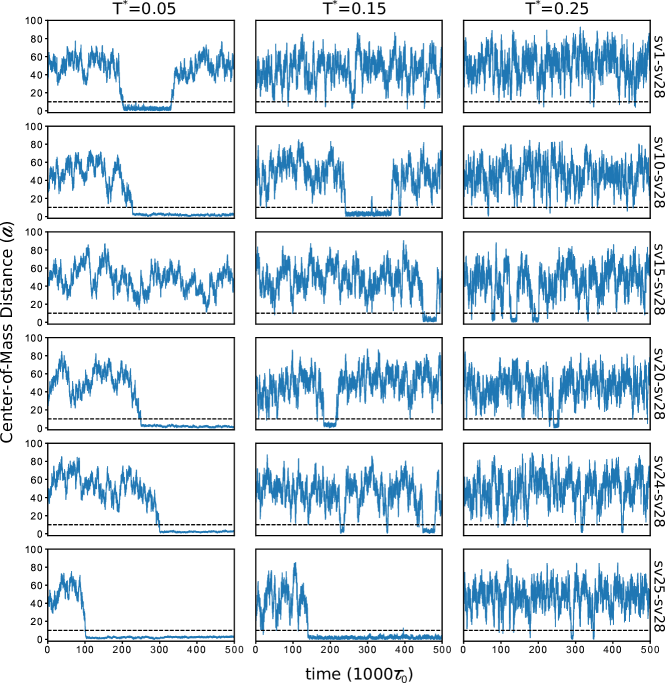
Figure S2: Time dependence of the center-of-mass separation $|{\bf R}_{\rm CM}^{AB}|$ between the two sequences ($A$, $B$) in the explicit-chain simulations of sv sequence pairs at $T^{*}=0.05$, $0.15$, and $0.25$ [$A=$ sv28, $B=$ (top to bottom) sv1, sv10, sv15, sv20, sv24, and sv25]. Dashed horizontal lines mark $|{\bf R}_{\rm CM}^{AB}|=10a$, the cutoff adopted in the present work for identifying a “bound state” of the two polyampholyte chains. None of the 18 center-of-mass distances plotted crosses the dashed lines more than five times, indicating potential limitations in sampling under thermodynamic equilibrium conditions.

For each simulation conducted for a given sv sequence pair, the simulated trajectory is examined for the center-of-mass separation between the two chain sequences to ascertain whether the chains form a binary complex in each and all snapshot collected. In the course of our investigation, we found that for simulations conducted at relatively low temperatures, $T^{*}<0.35$, there were only very limited jumps between an unbound state and what would be reasonably considered as the bound state (Fig. S2), suggesting that the simulated system may not have sufficient sampling at such low temperatures. We therefore focus on simulations conducted at $T^{*}\geq 0.35$.

Accordingly, the binding probabilities $\theta$ of the six pairs of sv sequences at $T^{*}=0.35$, $0.4$, $0.45$, and $0.5$ are calculated by the method described in the main text. As described there, we subtract a constant baseline collision probability, $\theta_{0}$, of two noninteracting monomer, where $\theta_{0}=[4\pi(10a)^{3}/3]/(100a)^{3}$, from the simulated bound-state ratio, and use $\tilde{\theta}=\theta-\theta_{0}$ to quantify the binding probability produced by interaction energies.

Combining the simulation results from $T^{*}=0.35$, $0.4$, $0.45$, and $0.5$, we estimate an enthalpic parameter $\Delta H$ and an entropic parameter $\Delta S$ for the binding for each of the six sv sequence pairs using the linear regression

$$\Delta H/T^{*}-\Delta S=\log(\theta^{-1}-1)\;,$$ (S29)

the results of which are reported in Table S2. The fitted $T^{*}$-dependent $\theta$s are then used to compute the corresponding $\tilde{\theta}$ values at the same $T^{*}$ for all sv sequence pairs to compare with the theory-predicted $K_{\rm D}$s in Fig. 7c and Fig. 9 of the main text.

[NaCl] (mM) Theory Theory H1-CTR Theory Net Charge ITC	[NaCl] (mM) smFRET
165 3.41 4.59 142 0.460.05 220 5.09 6.77 189 0.720.03 260 6.46 8.55 223 2.00.1 300 7.94 10.46 257 6.10.1 350 9.95 13.06 300 9.60.7	160 $(2.1^{+1.1}_{-0.8})\times 10^{-6}$ 180 $(3.7\!\pm\!0.5)\times 10^{-5}$ 205 $(1.0\!\pm\!0.1)\times 10^{-3}$ 240 $(2.5\!\pm\!0.3)\times 10^{-2}$ 290 0.230.15 330 0.140.04 340 0.40.18

Table S1: Theoretical and experimental ITC²⁴ and smFRET²³ $K_{\rm D}$s (in units of $\mu$M) of H1-ProT$\alpha$ fuzzy complexes at different NaCl concentrations ([NaCl] in mM). Amino acid sequences (in one-letter code) used in the theoretical calculation are taken from those studied by experiments, as follows (residues in red are not in the wildtype, they include those remaining after proteolytic cleavage of the HisTag).
ProT$\alpha$ (the “ProT$\alpha$ (without His-tag)” sequence in Ref. 24):
GSYMSDAAVDTSSEITTKDLKEKKEVVEEAENGRDAPANGNAENEENGEQEAD
NEVDEEEEEGGEEEEEEEEGDGEEEDGDEDEEAESATGKRAAEDDEDDDVDT
KKQKTDEDD;
H1 (from Ref. 24):
MTENSTSAPAAKPKRAKASKKSTDHPKYSDMIVAAIQAEKNRAGSSRQSIQKYIK
SHYKVGENADSQIKLSIKRLVTTGVLKQTKGVGASGSFRLAKSDEPKKSVAFKK
TKKELKKVATPKKASKPKKAASKAPTKKPKATPVKKTKKELKKVATPKKAKK
PKTVKAKPVKASKPKKAKPVKPKAKSSAKRAGKKKHHHHHH;
H1-CTR (H1-C-terminal region, from Ref. 23):
SVAFKKTKKEIKKVATPKKASKPKKAASKAPTKKPKATPVKKAKKKLAATP
KKAKKPKTVKAKPVKASKPKKAKPVKPKAKSSAKRAGKKKGGPR.
In the theoretical calculation, aspartic acid, glutamic acid (D, E) residues are each assigned $-1$ charge; arginine, lysine (R, K) residues are each assigned $+1$ charge; all other residue types are considered neutral ($0$ charge). The “Theory” results in the table are calculated using both terms for $B_{2}$ in Eq. 12 of the main text, whereas “Theory Net Charge” results are calculated using only the first term in the same equation. Because Eq. 12 relies on the Gaussian-chain approximation which may not be adequate for the N-terminal globular domain of H1, in addition to the data presented in Fig. 1 of the main text, we compute also $K_{\rm D}$s for the binding between the fully disordered C-terminal region of H1 (termed H1-CTR) with ProT$\alpha$ using both terms for $B_{2}$ in Eq. 12 of the main text and the 95-residue sequence for H1-CTR listed above. The resulting $K_{\rm D}$s listed under “Theory H1-CTR” in this table are about 1.2–1.5 times higher than those of full-length H1. This difference in ProT$\alpha$ binding between full-length and C-terminal H1 is likely attributable to the subtraction of the $+18$ charges in its N-terminal domain ²³.

Sequence $\theta|_{T^{*}=0.35}$ $\theta|_{T^{*}=0.40}$ $\theta|_{T^{*}=0.45}$ $\theta|_{T^{*}=0.50}$ $\Delta H$ $\Delta S$ $r^{2}$ sv1 0.362 % 0.432 % 0.420 % 0.252 % $-0.295$ $-6.32$ 0.225 sv10 0.736 % 0.743 % 0.591 % 0.351 % $-0.810$ $-7.08$ 0.720 sv15 1.01 % 1.64 % 0.923 % 0.803 % $-0.383$ $-5.46$ 0.202 sv20 0.812 % 1.34 % 0.381 % 0.700 % $-0.594$ $-6.33$ 0.178 sv24 4.04 % 1.83 % 2.56 % 0.976 % $-1.39$ $-7.17$ 0.703 sv25 3.00 % 0.590 % 0.912 % 0.228 % $-2.59$ $-11.1$ 0.787

Table S2: Simulated binding data and regression parameters; $r^{2}$ is square of Pearson correlation coefficient of the regression.

References

- Dunker et al. 2001 Dunker, A. K.; Lawson, J. D.; Brown, C. J.; Williams, R. M.; Romero, P.; Oh, J. S.; Oldfield, C. J.; Campen, A. M.; Ratliff, C. R.; Hipps, K. W. et al. Intrinsically disordered protein. J. Mol. Graphics & Modelling 2001, 19, 26–59
- van der Lee et al. 2014 van der Lee, R.; Buljan, M.; Lang, B.; Weatheritt, R. J.; Daughdrill, G. W.; Dunker, A. K.; Fuxreiter, M.; Gough, J.; Gsponer, J.; Jones, D. T. et al. Classification of intrinsically disordered regions and proteins. Chem. Rev. 2014, 114, 6589–6631
- Uversky 2002 Uversky, V. N. Natively unfolded proteins: A point where biology waits for physics. Protein Sci. 2002, 11, 739–756
- Wright and Dyson 2009 Wright, P. E.; Dyson, H. J. Linking folding and binding. Curr. Opin. Struct. Biol. 2009, 19, 31–38
- Bah et al. 2015 Bah, A.; Vernon, R. M.; Siddiqui, Z.; Krzeminski, M.; Muhandiram, R.; Zhao, C.; Sonenberg, N.; Kay, L. E.; Forman-Kay, J. D. Folding of an intrinsically disordered protein by phosphorylation as a regulatory switch. Nature 2015, 519, 106–109
- Marsh et al. 2012 Marsh, J. A.; Teichmann, S. A.; Forman-Kay, J. D. Probing the diverse landscape of protein flexibility and binding. Curr. Opin. Struct. Biol. 2012, 22, 643–650
- Borg et al. 2007 Borg, M.; Mittag, T.; Pawson, T.; Tyers, M.; Forman-Kay, J. D.; Chan, H. S. Polyelectrostatic interactions of disordered ligands suggest a physical basis for ultrasensitivity. Proc. Natl. Acad. Sci. U. S. A. 2007, 104, 9650–9655
- Mittag et al. 2008 Mittag, T.; Orlicky, S.; Choy, W.-Y.; Tang, X.; Lin, H.; Sicheri, F.; Kay, L. E.; Tyers, M.; Forman-Kay, J. D. Dynamic equilibrium engagement of a polyvalent ligand with a single-site receptor. Proc. Natl. Acad. Sci. U. S. A. 2008, 105, 17772–17777
- Tompa and Fuxreiter 2008 Tompa, P.; Fuxreiter, M. Fuzzy complexes: polymorphism and structural disorder in protein-protein interactions. Trends Biochem. Sci. 2008, 33, 2–8
- Sharma et al. 2015 Sharma, R.; Raduly, Z.; Miskei, M.; Fuxreiter, M. Fuzzy complexes: Specific binding without complete folding. FEBS Lett. 2015, 589, 2533–2542
- Miskei et al. 2017 Miskei, M.; Antal, C.; Fuxreiter, M. FuzDB: Database of fuzzy complexes, a tool to develop stochastic structure-function relationships for protein complexes and higher-order assemblies. Nucl. Acids Res. 2017, 45, D228–D235
- Arbesú et al. 2018 Arbesú, M.; Iruela, G.; Fuentes, H.; Teixeira, J. M. C.; Pons, M. Intramolecular fuzzy interactions involving intrinsically disordered domains. Front. Mol. Biosci. 2018, 5, 39
- Csizmok et al. 2017 Csizmok, V.; Orlicky, S.; Cheng, J.; Song, J.; Bah, A.; Delgoshaie, N.; Lin, H.; Mittag, T.; Sicheri, F.; Chan, H. S. et al. An allosteric conduit facilitates dynamic multisite substrate recognition by the SCFCdc4 ubiquitin ligase. Nat. Comm. 2017, 8, 13943
- Song et al. 2013 Song, J.; Ng, S. C.; Tompa, P.; Lee, K. A. W.; Chan, H. S. Polycation- interactions are a driving force for molecular recognition by an intrinsically disordered oncoprotein family. PLoS Comput. Biol. 2013, 9, e1003239
- Chen et al. 2015 Chen, T.; Song, J.; Chan, H. S. Theoretical perspectives on nonnative interactions and intrinsic disorder in protein folding and binding. Curr. Opin. Struct. Biol. 2015, 30, 32–42
- Lin et al. 2017 Lin, Y.-H.; Brady, J. P.; Forman-Kay, J. D.; Chan, H. S. Charge pattern matching as a ‘fuzzy’ mode of molecular recognition for the functional phase separations of intrinsically disordered proteins. New J. Phys. 2017, 19, 115003
- Perry and Sing 2020 Perry, S. L.; Sing, C. E. 100th Anniversary of macromolecular science viewpoint: Opportunities in the physics of sequence-defined polymers. ACS Macro Lett. 2020, 9, 216–225
- Sigalov 2016 Sigalov, A. B. Structural biology of intrinsically disordered proteins: Revisiting unsolved mysteries. Biochimie 2016, 125, 112–118
- Schuler et al. 2020 Schuler, B.; Borgia, A.; Borgia, M. B.; Heidarsson, P. O.; Holmstrom, E. D.; Nettels, D.; Sottini, A. Binding without folding — the biomolecular function of disordered polyelectrolyte complexes. Curr. Opin. Struct. Biol. 2020, 60, 66–76
- Sigalov et al. 2007 Sigalov, A. B.; Zhuravleva, A. V.; Orekhov, V. Y. Binding of intrinsically disordered proteins is not necessarily accompanied by a structural transition to a folded form. Biochimie 2007, 89, 419–421
- Danielsson et al. 2008 Danielsson, J.; Liljedahl, L.; Bárány-Wallje, L.; Sønderby, P.; Kristensen, L. H.; Martinez-Yamout, M. A.; Dyson, H. J.; Wright, P. E.; Poulsen, F. M.; Mäler, L. et al. The intrinsically disordered RNR inhibitor Sml1 is a dynamic dimer. Biochemistry 2008, 47, 13428–13437
- Nourse and Mittag 2014 Nourse, A.; Mittag, T. The cytoplasmic domain of the T-cell receptor zeta subunit does not form disordered dimers. J. Mol. Biol. 2014, 426, 62–70
- Borgia et al. 2018 Borgia, A.; Borgia, M. B.; Bugge, K.; Kissling, V. M.; Heidarsson, P. O.; Fernandes, C. B.; Sottini, A.; Soranno, A.; Buholzer, K. J.; Nettels, D. et al. Extreme disorder in an ultrahigh-affinity protein complex. Nature 2018, 555, 61–66
- Feng et al. 2018 Feng, H.; Zhou, B.-R.; Bai, Y. Binding affinity and function of the extremely disordered protein complex containing human linker histone H1.0 and its chaperone ProT. Biochemistry 2018, 57, 6645–6648
- Yang et al. 2019 Yang, J.; Zeng, Y.; Liu, Y.; Gao, M.; Liu, S.; Su, Z.; Huang, Y. Electrostatic interactions in molecular recognition of intrinsically disordered proteins. J. Biomol. Struct. Dyn. 2019, 11, 1–12
- Wang et al. 2018 Wang, J.; Choi, J.-M.; Holehouse, A. S.; Lee, H. O.; Zhang, X.; Jahnel, M.; Maharana, S.; Lemaitre, R.; Pozniakovsky, A.; Drechsel, D. et al. A molecular grammar governing the driving forces for phase separation of prion-like RNA binding proteins. Cell 2018, 174, 688–699.e16
- Tsang et al. 2019 Tsang, B.; Arsenault, J.; Vernon, R. M.; Lin, H.; Sonenberg, N.; Wang, L.-Y.; Bah, A.; Forman-Kay, J. D. Phosphoregulated FMRP phase separation models activity-dependent translation through bidirectional control of mRNA granule formation. Proc. Natl. Acad. Sci. U. S. A. 2019, 4218–4227
- Das and Pappu 2013 Das, R. K.; Pappu, R. V. Conformations of intrinsically disordered proteins are influenced by linear sequence distributions of oppositely charged residues. Proc. Natl. Acad. Sci. U. S. A. 2013, 110, 13392–13397
- Sawle and Ghosh 2015 Sawle, L.; Ghosh, K. A theoretical method to compute sequence dependent configurational properties in charged polymers and proteins. J. Chem. Phys. 2015, 143, 085101
- Lin and Chan 2017 Lin, Y.-H.; Chan, H. S. Phase separation and single-chain compactness of charged disordered proteins are strongly correlated. Biophys. J. 2017, 112, 2043–2046
- Zheng et al. 2020 Zheng, W.; Dignon, G.; Brown, M.; Kim, Y. C.; Mittal, J. Hydropathy patterning complements charge patterning to describe conformational preferences of disordered proteins. J. Phys. Chem. Lett. 2020, 11, 3408–3415
- Nott et al. 2015 Nott, T. J.; Petsalaki, E.; Farber, P.; Jervis, D.; Fussner, E.; Plochowietz, A.; Craggs, T. D.; Bazett-Jones, D. P.; Pawson, T.; Forman-Kay, J. D. et al. Phase transition of a disordered nuage protein generates environmentally responsive membraneless organelles. Mol. Cell 2015, 57, 936–947
- Lin et al. 2016 Lin, Y.-H.; Forman-Kay, J. D.; Chan, H. S. Sequence-specific polyampholyte phase separation in membraneless organelles. Phys. Rev. Lett. 2016, 117, 178101
- Pak et al. 2016 Pak, C. W.; Kosno, M.; Holehouse, A. S.; Padrick, S. B.; Mittal, A.; Ali, R.; Yunus, A. A.; Liu, D. R.; Pappu, R. V.; Rosen, M. K. Sequence determinants of intracellular phase separation by complex coacervation of a disordered protein. Mol. Cell 2016, 63, 72–85
- Lin et al. 2017 Lin, Y.-H.; Song, J.; Forman-Kay, J. D.; Chan, H. S. Random-phase-approximation theory for sequence-dependent, biologically functional liquid-liquid phase separation of intrinsically disordered proteins. J. Mol. Liq. 2017, 228, 176–193
- Lytle and Sing 2017 Lytle, T. K.; Sing, C. E. Transfer matrix theory of polymer complex coacervation. Soft Matter 2017, 13, 7001–7012
- Chang et al. 2017 Chang, L.-W.; Lytle, T. K.; Radhakrishna, M.; Madinya, J. J.; Vélez, J.; Sing, C. E.; Perry, S. L. Sequence and entropy-based control of complex coacervates. Nat. Comm. 2017, 8, 1273
- Das et al. 2018 Das, S.; Amin, A. N.; Lin, Y.-H.; Chan, H. S. Coarse-grained residue-based models of disordered protein condensates: Utility and limitations of simple charge pattern parameters. Phys. Chem. Chem. Phys. 2018, 20, 28558–28574
- McCarty et al. 2019 McCarty, J.; Delaney, K. T.; Danielsen, S. P. O.; Fredrickson, G. H.; Shea, J.-E. Complete phase diagram for liquid–liquid phase separation of intrinsically disordered proteins. J. Phys. Chem. Lett. 2019, 10, 1644–1652
- Statt et al. 2020 Statt, A.; Casademunt, H.; Brangwynne, C. P.; Panagiotopoulos, A. Z. Model for disordered proteins with strongly sequence-dependent liquid phase behavior. J. Chem. Phys. 2020, 152, 075101
- Schuster et al. 2020 Schuster, B. S.; Dignon, G. L.; Tang, W. S.; Kelley, F. M.; Ranganath, A. K.; Jahnke, C. N.; Simplins, A. G.; Regy, R. M.; Hammer, D. A.; Good, M. C. et al. Identifying sequence perturbations to an intrinsically disordered protein that determine its phase separation behavior. Proc. Natl. Acad. Sci. U. S. A. 2020, 117, 11421–11431
- Das et al. 2018 Das, S.; Eisen, A.; Lin, Y.-H.; Chan, H. S. A lattice model of charge-pattern-dependent polyampholyte phase separation. J. Phys. Chem. B 2018, 122, 5418–5431
- Zarin et al. 2019 Zarin, T.; Strome, B.; Nguyen Ba, A. N.; Alberti, S.; Forman-Kay, J. D.; Moses, A. M. Proteome-wide signatures of function in highly diverged intrinsically disordered regions. eLife 2019, 8, e46883
- Panagiotopoulos et al. 1998 Panagiotopoulos, A. Z.; Wong, V.; Floriano, M. A. Phase equilibria of lattice polymers from histogram reweighting Monte Carlo simulations. Macromolecules 1998, 31, 912–918
- Wang and Wang 2014 Wang, R.; Wang, Z.-G. Theory of polymer chains in poor solvent: Single-chain structure, solution thermodynamics, and point. Macromolecules 2014, 47, 4094–4102
- Dignon et al. 2018 Dignon, G. L.; Zheng, W.; Best, R. B.; Kim, Y. C.; Mittal, J. Relation between single-molecule properties and phase behavior of intrinsically disordered proteins. Proc. Natl. Acad. Sci. U. S. A. 2018, 115, 9929–9934
- Lin et al. 2020 Lin, Y.-H.; Brady, J. P.; Chan, H. S.; Ghosh, K. A unified analytical theory of heteropolymers for sequence-specific phase behaviors of polyelectrolytes and polyampholytes. J. Chem. Phys. 2020, 152, 045102
- Pathria 2006 Pathria, R. K. Statistical Mechanics, 2nd Ed.; Elsevier, 2006
- Smith et al. 2016 Smith, A. M.; Lee, A. A.; Perkin, S. The electrostatic screening length in concentrated electrolytes increases with concentration. J. Phys. Chem. Lett. 2016, 7, 2157–2163
- Chowdhury et al. 2020 Chowdhury, A.; Sottini, A.; Borgia, A.; Borgia, M. B.; Nettels, D.; Schuler, B. Thermodynamics of the interaction between biological polyelectrolyte-like disordered proteins: From binary complexes to oligomers. Biophys. J. 2020, 118, Supplement 1, 215A
- Muthukumar 2017 Muthukumar, M. 50th anniversary perspective: A perspective on polyelectrolyte solutions. Macromolecules 2017, 50, 9528–9560
- McCammon et al. 1979 McCammon, J. A.; Wolynes, P. G.; Karplus, M. Picosecond dynamics of tyrosine side chains in proteins. Biochemistry 1979, 18, 927–942
- Jha and Freed 2008 Jha, A. K.; Freed, K. F. Solvation effect on conformations of 1,2:dimethoxyethane: Charge-dependent nonlinear response in implicit solvent models. J. Chem. Phys. 2008, 128, 034501
- Ng and Geller 1969 Ng, E. W.; Geller, M. A table of integrals of the error functions. J. Res. Natl. Inst. Stand.—B. Math. Sci. 1969, 73B, 1–20
- Ermoshkin and Olvera de la Cruz 2003 Ermoshkin, A. V.; Olvera de la Cruz, M. Polyelectrolytes in the presence of multivalent ions: gelation versus segregation. Phys. Rev. Lett. 2003, 90, 125504
- Danielsen et al. 2019 Danielsen, S. P. O.; McCarty, J.; Shea, J.-E.; Delaney, K. T.; Fredrickson, G. H. Molecular design of self-coacervation phenomena in block polyampholytes. Proc. Natl. Acad. Sci. U. S. A. 2019, 116, 8224–8232
- Shen and Wang 2018 Shen, K.; Wang, Z.-G. Polyelectrolyte chain structure and solution phase behavior. Macromolecules 2018, 51, 1706–1717
- Huihui and Ghosh 2020 Huihui, J.; Ghosh, K. An analytical theory to describe sequence-specific inter-residue distance profiles for polyampholytes and intrinsically disordered proteins. J. Chem. Phys 2020, 152, 161102
- Riback et al. 2017 Riback, J. A.; Katanski, C. D.; Kear-Scott, J. L.; Pilipenko, E. V.; Rojek, A. E.; Sosnick, T. R.; Drummond, D. A. Stress-triggered phase separation is an adaptive, evolutionarily tuned response. Cell 2017, 168, 1028–1040
- Chou and Aksimentiev 2020 Chou, H.-Y.; Aksimentiev, A. Single-protein collapse determines phase equilibria of a biological condensate. J. Phys. Chem. Lett. 2020, 11, 4923–4929
- Zeng et al. 2020 Zeng, X.; Holehouse, A. S.; Chilkoti, A.; Mittag, T.; Pappu, R. V. Connecting coil-to-globule transitions to full phase diagrams for intrinsically disordered proteins. Biophys. J. 2020, 119, 1–17
- Chan and Dill 1991 Chan, H. S.; Dill, K. A. Sequence space soup of proteins and copolymers. J. Chem. Phys. 1991, 95, 3775–3787
- O’Toole and Panagiotopoulos 1992 O’Toole, E. M.; Panagiotopoulos, A. Z. Monte Carlo simulation of folding transitions of simple model proteins using a chain growth algorithm. J. Chem. Phys. 1992, 97, 8644–8652
- Weeks et al. 1971 Weeks, J. D.; Chandler, D.; Andersen, H. C. Role of repulsive forces in determining the equilibrium structure of simple liquids. J. Chem. Phys. 1971, 54, 5237–5247
- Silmore et al. 2017 Silmore, K. S.; Howard, M. P.; Panagiotopoulos, A. Z. Vapour-liquid phase equilibrium and surface tension of fully flexible Lennard-Jones chains. Mol. Phys. 2017, 115, 320–327
- Mundy et al. 1995 Mundy, C. J.; Siepmann, J. I.; Klein, M. L. Calculation of the shear viscosity of decane using a reversible multiple time‐step algorithm. J. Chem. Phys. 1995, 102, 3376–3380
- Martin and Siepmann 1998 Martin, M. G.; Siepmann, J. I. Transferable potentials for phase equilibria. 1. United-atom description of n-alkanes. J. Phys. Chem. B 1998, 102, 2569–2577
- Nicolas and Smit 2002 Nicolas, J. P.; Smit, B. Molecular dynamics simulations of the surface tension of n-hexane, n-decane and n-hexadecane. Mol. Phys. 2002, 100, 2471–2475
- Pàmies et al. 2003 Pàmies, J. C.; McCabe, C.; Cummings, P. T.; Vega, L. F. Coexistence densities of methane and propane by canonical molecular dynamics and gibbs ensemble Monte Carlo simulations. Mol. Simul. 2003, 29, 463–470
- Anderson et al. 2008 Anderson, J. A.; Lorenz, C. D.; Travesset, A. General purpose molecular dynamics simulations fully implemented on graphics processing units. J. Comput. Phys. 2008, 227, 5342–5359
- Glaser et al. 2015 Glaser, J.; Nguyen, T. D.; Anderson, J. A.; Lui, P.; Spiga, F.; Millan, J. A.; Morse, D. C.; Glotzer, S. C. Strong scaling of general-purpose molecular dynamics simulations on GPUs. Comput. Phys. Comm. 2015, 192, 97–107
- LeBard et al. 2012 LeBard, D. N.; Levine, B. G.; Mertmann, P.; Barr, S. A.; Jusufi, A.; Sanders, S.; Klein, M. L.; Panagiotopoulos, A. Z. Self-assembly of coarse-grained ionic surfactants accelerated by graphics processing units. Soft Matter 2012, 8, 2385–2397