Projection evolution and quantum spacetime

Abstract

We discuss the problem of time in quantum mechanics. In the traditional formulation time enters the model as a parameter, not an observable. In our model time is a quantum observable as any other quantum quantity and it is also a component of the spacetime position operator. In this case, instead of the unitary time evolution, other operators, usually projection or POVM operators which map the space of initial states into the space of final states at each step of the evolution can be used. The quantum evolution itself is a stochastic process. This allows to treat time as a quantum observable in a consistent, observer independent way, which is a very important feature to resolve some quantum paradoxes and the time problem in cosmology.

An idea of construction of a quantum spacetime as a special set of the allowed states is presented. An example of a structureless quantum Minkowski–like spacetime is also considered.

We present the projection evolution model and show how the traditional Schrödinger evolution and relativistic equations can be obtained from it, in the flat structureless spacetime.

We propose the form of the time operator which satisfies the energy-time uncertainty relation based on the same inequality as the space position and spatial momenta observables. The sign of the temporal component of the four-momentum operator defines the basic arrow of time in spacetime.

1 Introduction

For many years time was treated in physics as a universal parameter which allows the observer to divide the reality into past, present, and future. What is more, time was flowing always in one direction, called the arrow of time. This direction implied also the direction of changes that may spontaneously happen to any physical system, which ultimately leads to the notion of causality. We are used to the fact that past affects future, but future cannot affect the past, as this will act against the arrow of time.

The development of relativity theory changed this picture in a substantial way. To obtain a realistic model one needs to treat time and space in a way consistent with the relativity theory. The metric and other tensors gained their time components which were transforming during the change of the coordinate system along with the spatial coordinates. For example, the position and the linear momentum are four-vectors $x^{\mu}$ and $p^{\mu}$, $\mu=0,1,2,3$. They take the form $x^{\mu}=(x^{0},\vec{x})$ and $p^{\mu}=(p^{0},\vec{p})$, where $x^{0}$ represents time and $p^{0}=E/c$, $E$ being the total energy. This feature is absent in the non-relativistic physics.

One may ask if time and space positions behave in the same way in the macroscopic and microscopic scales? We know that both non-relativistic and relativistic physics agree upon the basic properties of time, so if one expects any deviations from the standard picture, one should look at quantum mechanics.

In the standard formulation of the quantum theory, any physical quantity is represented by a self adjoint operator whose eigenvalues are the possible outcomes of its measurement. However, the so-called Pauli theorem [1, 2] states, that it is impossible to construct a self adjoint time operator which would be canonically conjugate to the Hamiltonian. It follows that time is not a physical observable but is introduced as a universal numerical parameter. This approach is inconsistent with what we know from the relativity theory, not to mention that it gives very limited means to discuss quantum events in the time domain. A careful mathematical analysis of this problem was presented by E.A. Galapon in Ref. [3]. He showed that this problem can be overcome using weaker assumptions about the observables.

It has been extensively discussed how to introduce time as an observable in the theory, as this affects the construction of the arrow of time and clocks (see [4, 5, 6, 7, 8, 9, 10, 11, 12, 13, 14, 15, 16, 17, 18, 19, 20, 21, 22, 23, 24, 25, 26, 27, 28, 29, 30, 31, 32, 33, 34] for recent developments). Related topics include also the problem of time in entangled systems, the time of decoherence and the role of the energy-time uncertainty relation. The process of quantization can be performed in different ways and tested using specially designed experiments, like it has been shown in the example of the time of arrival operator [35, 36]. Since time is connected with the energy operator, thermodynamics of quantum processes started to be of interest [37, 38]. It has already been shown that due to the quantum correlations, heat may spontaneously flow from the colder to the hotter subsystem [39], which is not observed in the macroscopic scale. Entanglement and the immediate change of state of both entangled particles rises also the question how to describe [40, 41] and experimentally investigate [42] this process.

The problem of time appears also in systems performing quantum computation. Most quantum protocols assume that we can neglect the time delays introduced by quantum gates and connections in the system, which does not have to be the case. Another problem arises with the theoretically proposed quantum gates with feedback [43, 44, 45, 46], which are impossible to describe using standard tools. Understanding the time structure of quantum operations is also vital for constructing future quantum neural networks [47].

Treating time as an observable leads to the problem of time measurements [48], also in the context of quantum cosmology [49]. As time becomes a variable, new phenomena start to be possible, like dark matter described by fields evolving backwards in time [50].

The important role of time in quantum theories is suggested by some experiments. In Refs. [51, 52] J.A. Wheeler proposed a Gedankenexperiment, the so called “delayed choice problem”. This idea has been experimentally tested by the group of A. Aspect with the primary intention to test Bell’s inequalities [53] showing that Wheeler’s predictions were correct. Other groups [54, 55, 56, 57, 58, 59] arrived at similar results. In order to investigate the problem further, the quantum eraser was used [60, 61]. The effect was visible even when the changes introduced to the experimental setup led to acausal events.

Another experiment was conducted using entangled pairs of photons [62, 63] separated by 144 km. Even though the particles were causally disconnected, the changes made in the first laboratory were affecting the second particle.

If time in the quantum regime should be treated as a coordinate, and in fact a quantum observable, all physical objects’ states have to have some “width” in the time direction, which is related to the energy-time (more precisely – the temporal component of the four momentum operator versus time) uncertainty relation. This means that it should be possible to observe the interference of quantum objects through their overlap in time [64, 65, 66, 67]. It also means, that time cannot be treated as a parameter.

It seems to be very difficult to answer the fundamental question: What is time? An interesting hypothesis is presented in Ref. [68] in which the authors propose, that time is a consequence of the entanglement between particles in the universe.

Other proposal for introducing the quantuntum time is the relational quantum mechanics summarized in Ref. [32, 33, 34], see also references therein.

In this paper we present a consistent formulation of the quantum theory in which the spacetime can emerge from a set of observables supported by the quantum state space. It can be generated from a set of self-conjugated operators or operator valued measures having expected properties. As a byproduct, such construction should allow to obtain the time operator and the canonically conjugated observable which represents the temporal momentum.

In the PEv approach the evolution of quantum states has to be reformulated, as time, being a coordinate, cannot act as a universal ordering parameter any longer. However, we show that the traditional time evolution, like the Schrödinger, Klein-Gordon, Dirac and other equations of motion can be obtained as special cases within our model. The problem of symmetries and conservation laws during the evolution is also shortly discussed.

The Projection Evolution approach (PEv) is covariant, it does not need any external observer and similarly to relational dynamics no background is required. This implies that PEv formalism can also be applied in a natural way to quantum gravity.

2 Projection evolution of quantum systems

In quantum mechanics each physical system is described by a set of all possible observables which can be associated with it, see, e.g., the algebraic approach to quantum mechanics [69, 70, 71]. The observables themselves are represented either by self-adjoint operators or, more generally, by the appropriate operator valued measures (sharp or POVM). In traditional approaches to quantum mechanics time is not represented in the set of these observables, it is considered to be a parameter. This inconsistency leads to various quantum paradoxes and also to the time problem in gravity and cosmology; the extensive set of references for the latter problem can be found in Ref. [32, 33, 34].

One expects, the full set of observables of any physical system under consideration contains a subset of the spacetime position operators and their canonical conjugated momenta. Among them the time observable and its canonical conjugate is also expected. It follows that time cannot be considered as a parameter which enumerates subsequent events but it has to be represented by an operator or the appropriate operator measure similar to the position observables. It means that different time characteristics of a given quantum system can be calculated. In general, they are dependent on the state of this system.

The assumption that quantum time, and generally the spacetime, is “created” by changes of the Universe requires a modification of some parts of the paradigm of science related to the causality and the ordering of quantum events.

2.1 The changes principle

We start by formulating the fundamental principle of the projection evolution approach:

The evolution of a system is a random process caused by the spontaneous changes in the Universe.

We call it the changes principle. It means that we treat the change as the primary process, which allows to determine time, space and spacetime in terms of quantum observables.

This is in contradiction with the usual thinking in which the existence of time allows the changes to happen. In our approach the changes happen spontaneously, according to the probability distribution, which is dictated by many factors describing the Universe and in the case of the subsystems of this Universe also their environments. It does not mean that the changes of a quantum state are totally stochastic, without any constraints. They are obviously not deterministic, but because of interactions, symmetries which have to be conserved, EPR correlations etc., they are related to each other and bound by the rules of their behavior known from our experience.

As a consequence one may expect the existence of a kind of pseudo-causality based on the ordering of the quantum events, which leads to the causality principle in the case of macroscopic physical systems. In order to describe this property we introduce a parameter $\tau$ which orders quantum events. This parameter should be common for the whole Universe. It should take values from an ordered set but it does not need to have any metric structure. The parameter $\tau$ is not an additional dimension of our space and it is not a replacement of time. It serves only to enumerate the subsequent steps of the evolution of the Universe and any of its physical subsystems. The most natural linearly ordered set is any subset of the real numbers.

In what follows we assume that the domain of the evolution parameter $\tau$ is isomorphic to integers $\mathbb{Z}$ or their subset. In this case we can always use the notion of “the next step of the evolution,” which may be problematic for the real numbers. In the situation of a continuous or dense subset of the real numbers as the domain for $\tau$, there are some conceptual difficulties which should be, if needed, solved in the future.

An additional, very important feature of this approach is that this idea does not need the spacetime as the background, it is background independent. Most of the physical theories constructed till now use the spacetime as the primary object, with the dynamics built on top of it. In other words, the projection evolution approach is a background free theory. In addition, it does not need any external observer as time is an internal observable. This point is extremely important in the quantum gravity and cosmology.

2.2 Projection evolution operators

In the standard formulation of quantum physics, there are two kinds of time evolution: (i) the unitary evolution, which is a deterministic evolution of the actual quantum state, and (ii) the stochastic evolution, which takes place during a measurement. The latter process involves the projection of the quantum state onto the measured state and can be described by one of the projection postulates.

There is a common belief that every measurement process can be described by means of the unitary evolution of a larger system. This approach leads, however, to the known quantum measurement problems [72].

The changes principle is incompatible with the unitary evolution, where time is considered to be a parameter. The idea of the changes principle suggests the opposite scenario – the primary evolution is the stochastic evolution offered by a projection postulate. In the projection evolution formalism we propose to use the generalized form of the Lüders [73] type of the projection postulate.

One needs to notice that this mechanism defines events as subsequent steps of the evolution.

In the following, we introduce the evolution operators which are formally responsible for the quantum evolution of a physical object. In general these operators are different for different systems, similarly to the Hamiltonian, which is a characteristic object for a given quantum system. On the other hand one should, in principle, be able to construct the projection evolution operators for the whole Universe which will contain the operators for any smaller subsystem. It is due to the fact that the proposed formalism does not require any external observer and external variables for the evolution.

The projection evolution operator from the evolution step $\tau_{n-1}$ to the evolution step $\tau_{n}$, where $n\in\mathbb{Z}$, is a family of mappings from the space of quantum states at the evolution step $\tau_{n-1}$ to the space of quantum states at the evolution step $\tau_{n}$.

The appropriate state space, at the evolution step $\tau_{k}$, denoted by $\mathcal{T}^{+}_{1}(\mathcal{K}(\tau_{k}))$, is assumed to be the space of trace one, positive and self-adjoint operators acting in the Hilbert space $\mathcal{K}(\tau_{k})$ , i.e., it is the space of quantum density operators. Every corresponding Hilbert space $\mathcal{K}(\tau_{k})$, at the evolution step $\tau_{k}$, is a subspace of a single global Hilbert space $\mathcal{K}_{U}$.

Note, that in this case, the simplest Hilbert space of a single, spinless particle is not the space $L^{2}(\mathbb{R}^{3},d^{3}x)$ but the space $L^{2}(\mathbb{R}^{4},d^{4}x)$, where the fourth dimension is time, treated here on the same footing as the positions in the 3D-space. The fundamental difference is that the scalar procuct in $L^{2}(\mathbb{R}^{4},d^{4}x)$, which represents the probability amplitudes, contains integration over time – more discussion about this case is in Sec. 5.1.

These mappings can always be written in terms of the so-called quantum operations or their generalizations. The formalism of quantum operations was invented around 1983 by Krauss [74], who relied on the earlier mathematical works of Choi [75].

The projection evolution operators at the evolution step $\tau_{n}$ are formally defined as a family of transformations from the quantum state space (density operators space) $\mathcal{T}^{+}_{1}(\mathcal{K}(\tau_{n-1}))$ to the space $\mathcal{T}^{+}(\mathcal{K}(\tau_{n}))$,

$$\mathsf{F}\kern-1.0pt\hbox to0.0pt{\hss$|$}(\tau_{n};\nu,\cdot):\mathcal{T}^{+}_{1}(\mathcal{K}(\tau_{n-1}))\rightarrow\mathcal{T}^{+}(\mathcal{K}(\tau_{n})),$$ (1)

where $\mathcal{T}^{+}(\mathcal{K}(\tau))$ is the space of finite trace, positive and self-adjoint operators acting in the Hilbert space $\mathcal{K}(\tau)$, $\nu\in{\cal Q}_{n}$, with ${\cal Q}_{n}\equiv{\cal Q}_{\tau_{n}}$ being a family of sets of quantum numbers defining potentially available final states for the evolution from $\tau_{n-1}$ to $\tau_{n}$.

We denote by $\mathsf{F}\kern-1.0pt\hbox to0.0pt{\hss$|$}(\tau_{n};\nu,\rho)$ the result of the action of the operator $\mathsf{F}\kern-1.0pt\hbox to0.0pt{\hss$|$}(\tau_{n};\nu,\cdot)$ on the density operator $\rho$, such that $\mathsf{F}\kern-1.0pt\hbox to0.0pt{\hss$|$}(\tau_{n};\nu,\cdot)\rho=\mathsf{F}\kern-1.0pt\hbox to0.0pt{\hss$|$}(\tau_{n};\nu,\rho)$. The notation $\mathsf{F}\kern-1.0pt\hbox to0.0pt{\hss$|$}(\tau_{n};\nu,\rho)$ is in some cases more appropriate because, in general, the changes principle does not constrain the evolution operators to be linear.

To use the generalized Lüders projection postulate as the principle for the evolution, the operators $\mathsf{F}\kern-1.0pt\hbox to0.0pt{\hss$|$}(\tau_{n};\nu,\rho)$ have to be self-adjoint, non-negative, and with finite trace:

$$\mathsf{F}\kern-1.0pt\hbox to0.0pt{\hss$|$}(\tau;\nu,\rho)^{\dagger}=\mathsf{F}\kern-1.0pt\hbox to0.0pt{\hss$|$}(\tau;\nu,\rho),$$ (2)

$$\mathsf{F}\kern-1.0pt\hbox to0.0pt{\hss$|$}(\tau;\nu,\rho)\geq 0,$$ (3)

$$\sum_{\nu\in{\cal Q}_{\tau}}\mathrm{Tr}(\mathsf{F}\kern-1.0pt\hbox to0.0pt{\hss$|$}(\tau;\nu,\rho))<\infty,$$ (4)

for every state $\rho$. These three conditions allow $\mathsf{F}\kern-1.0pt\hbox to0.0pt{\hss$|$}$ to transform the density operator $\rho$ into another density operator, as is shown in Eq. (5) below.

Assume that at the evolution step $\tau_{n-1}$ the actual quantum state of a physical system is given by the density operator $\rho(\tau_{n-1};\nu_{n-1})$, with $\nu_{n-1}\in{\cal Q}_{n-1}$. The changes principle implies that every step of the evolution is similar to the measurement process in the sense that there exists a mechanism in the Universe, the chooser, which chooses randomly from the set of states determined by the projection postulates the next state of the system for $\tau=\tau_{n}$. With these assumptions, following Ref. [73], we postulate $\rho(\tau_{n};\nu_{n})$, $\nu_{n}\in{\cal Q}_{n}$, in the form

$$\rho(\tau_{n};\nu_{n})=\frac{\mathsf{F}\kern-1.0pt\hbox to0.0pt{\hss$|$}(\tau_{n};\nu_{n},\rho(\tau_{n-1};\nu_{n-1}))}{\textrm{Tr}\left(\mathsf{F}\kern-1.0pt\hbox to0.0pt{\hss$|$}(\tau_{n};\nu_{n},\rho(\tau_{n-1};\nu_{n-1}))\right)}.$$ (5)

Because the chooser represents a stochastic process, to fully describe it one needs to determine the probability distribution for getting a given state in the next step of the evolution. An example of an evolution path is presented in Fig. 1 by the solid line. The dotted lines show other potential paths.

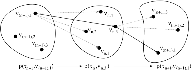
Figure 1: The density matrix $\rho$ is randomly chosen at each evolution step $\tau$ from the possible states labeled by $\mathcal{Q}_{m}=\{\nu_{m,1},\nu_{m,2},\dots\}$, where $m=n-1,n,n+1$.

In general, the probability distribution for the chooser is given by the quantum mechanical transition probability from the previous to the next state. This probability for pure quantum states is determined by the appropriate probability amplitudes in the form of scalar products. The transition probability among mixed states, in general, remains an open problem, see e.g. [76, 77].

We denote the transition probability (or the transition probability density) from the state labelled by the set of quantum numbers $\nu_{n-1}$ at $\tau_{n-1}$ to the state labelled by the set of quantum numbers $\nu_{n}$ at $\tau_{n}$ for a given evolution process by $\mathrm{pev}\kern-2.0pt\left(\nu_{n-1}\to\nu_{n}\right)$. The arguments of $\mathrm{pev}\kern-2.0pt\left(\right)$ indicate the initial and the final state of the transition.

The most important realization of the evolution operators $\mathsf{F}\kern-1.0pt\hbox to0.0pt{\hss$|$}(\tau_{n};\nu_{n},\rho)$ can be constructed from the density matrix $\rho$ and some operators $\mathsf{E}\kern-1.0pt\hbox to0.0pt{\hss$|$}$ in the following form: for every $\nu_{n}\in{\cal Q}_{n}$ we have

$$\mathsf{F}\kern-1.0pt\hbox to0.0pt{\hss$|$}(\tau_{n};\nu_{n},\rho)=\sum_{\alpha}\mathsf{E}\kern-1.0pt\hbox to0.0pt{\hss$|$}(\tau_{n};\nu_{n},\alpha)\ \rho\ \mathsf{E}\kern-1.0pt\hbox to0.0pt{\hss$|$}(\tau_{n};\nu_{n},\alpha)^{\dagger},$$ (6)

where the summation over $\alpha$ is dependent on the quantum numbers $\nu_{n}$. It is easy to check that the conditions (2) and (3) are automatically fulfilled, namely:

$$\mathsf{F}\kern-1.0pt\hbox to0.0pt{\hss$|$}(\tau_{n};\nu_{n},\rho)^{\dagger}=\sum_{\alpha}\mathsf{E}\kern-1.0pt\hbox to0.0pt{\hss$|$}(\tau_{n};\nu_{n},\alpha)\ \rho\ \mathsf{E}\kern-1.0pt\hbox to0.0pt{\hss$|$}(\tau_{n};\nu_{n},\alpha)^{\dagger}=\mathsf{F}\kern-1.0pt\hbox to0.0pt{\hss$|$}(\tau_{n};\nu_{n},\rho)$$ (7)

and, since $\rho\geq 0$, we have for all $\phi\in\mathcal{K}$

$$\langle\phi|\sum_{\alpha}\mathsf{E}\kern-1.0pt\hbox to0.0pt{\hss$|$}(\tau_{n};\nu_{n},\alpha)\ \rho\ \mathsf{E}\kern-1.0pt\hbox to0.0pt{\hss$|$}(\tau_{n};\nu_{n},\alpha)^{\dagger}|\phi\rangle$$

$$=\sum_{\alpha}\langle\phi|\mathsf{E}\kern-1.0pt\hbox to0.0pt{\hss$|$}(\tau_{n};\nu_{n},\alpha)\ \rho\ \mathsf{E}\kern-1.0pt\hbox to0.0pt{\hss$|$}(\tau_{n};\nu_{n},\alpha)^{\dagger}|\phi\rangle\geq 0.$$ (8)

Using Eq. (6) and the fact that trace is cyclic, the left hand side of the condition (4) takes the form

$$\sum_{\nu_{n}\in{\cal Q}_{n}}\sum_{\alpha}\mathrm{Tr}(\mathsf{E}\kern-1.0pt\hbox to0.0pt{\hss$|$}(\tau_{n};\nu_{n},\alpha)\ \rho\ \mathsf{E}\kern-1.0pt\hbox to0.0pt{\hss$|$}(\tau_{n};\nu_{n},\alpha)^{\dagger})$$

$$=\sum_{\nu_{n}\in{\cal Q}_{n}}\mathrm{Tr}\left(\sum_{\alpha}\mathsf{E}\kern-1.0pt\hbox to0.0pt{\hss$|$}(\tau_{n};\nu_{n},\alpha)^{\dagger}\mathsf{E}\kern-1.0pt\hbox to0.0pt{\hss$|$}(\tau_{n};\nu_{n},\alpha)\ \rho\right)<\infty$$ (9)

Typical and useful examples of the $\mathsf{E}\kern-1.0pt\hbox to0.0pt{\hss$|$}$ operators are connected with the unitary evolution and the orthogonal resolution of unity. In the first case the operator is

$$\mathsf{E}\kern-1.0pt\hbox to0.0pt{\hss$|$}(\tau_{n};\nu_{n0},\alpha_{0})=U(\tau_{n}),$$ (10)

where $\nu_{n0}$ and $\alpha_{0}$ are some fixed values of $\nu_{n}$ and $\alpha$, and $U(\tau_{n})$ is a unitary operator. In this case, following Eq. (6), the next step of the evolution is chosen uniquely with the probability equal to 1, as

$$\rho(\tau_{n};\nu_{n})=U(\tau_{n})\ \rho(\tau_{n-1};\nu_{n-1})\ U(\tau_{n})^{\dagger}.$$ (11)

One needs to note that the unitary operator (10) is not parametrized by time but by the evolution parameter $\tau$, even though, in general, it is time dependent .

The PEv approach allows for the generalization of the idea of the unitary evolution. For example, it is possible to consider the case when a few different unitary evolution channels are opened, each with a given probability $p_{m}$. In this case, the state for the evolution step $n$ is a linear combination of the products of different unitary evolutions of the previous state,

$$\rho(\tau_{n};\nu_{n})=\sum_{m=1}^{N}p_{m}\,U_{m}(\tau_{n})\rho(\tau_{n-1};\nu_{n-1})U_{m}(\tau_{n})^{\dagger}\,,$$ (12)

where $U_{m}^{\dagger}=U_{m}^{-1}$ for $m=1,\dots,N$.

In the case of the orthogonal resolution of unity with respect to the quantum numbers $\nu_{n}$ the following conditions hold (we have fixed for simplicity the $\alpha$ parameter and omitted it in the notation, but the more general case can be written similarly):

$$\mathsf{E}\kern-1.0pt\hbox to0.0pt{\hss$|$}(\tau_{n};\nu_{n})^{\dagger}=\mathsf{E}\kern-1.0pt\hbox to0.0pt{\hss$|$}(\tau_{n};\nu_{n}),$$

$$\mathsf{E}\kern-1.0pt\hbox to0.0pt{\hss$|$}(\tau_{n};\nu_{n})\mathsf{E}\kern-1.0pt\hbox to0.0pt{\hss$|$}(\tau_{n};\nu_{n}^{\prime})=\delta_{\nu_{n}\nu_{n}^{\prime}}\mathsf{E}\kern-1.0pt\hbox to0.0pt{\hss$|$}(\tau_{n};\nu_{n}),$$

$$\sum_{\nu_{n}\in{\cal Q}_{n}}\mathsf{E}\kern-1.0pt\hbox to0.0pt{\hss$|$}(\tau_{n};\nu_{n})=1\kern-4.5pt1,$$ (13)

where $1\kern-4.5pt1$ denotes the unit operator. Different alternatives of choices of the quantum states are described by different sets of quantum numbers $\nu_{n}$.

The probability distribution of choosing the next state of the evolution generated by (2.2) is now given by the known quantum mechanical formula:

$$\mathrm{pev}\kern-2.0pt\left(\nu_{n-1}\to\nu_{n}\right)=\mathrm{Tr}\left(\mathsf{E}\kern-1.0pt\hbox to0.0pt{\hss$|$}(\tau_{n};\nu_{n})\ \rho(\tau_{n-1},\nu_{n-1})\ \mathsf{E}\kern-1.0pt\hbox to0.0pt{\hss$|$}(\tau_{n};\nu_{n})^{\dagger}\right).$$ (14)

The above discussed examples, even though generic for many quantum mechanical systems, are only special cases of the more general evolution operators.

3 The quantum spacetime

To simplifiy notation, we consider in this section a single evolution step only, i.e., we keep the evolution parameter $\tau$ fixed. The quantum spacetime, similarly to other properties of any quantum system can change from one to another step of its evolution.

The projection evolution is compatible with any reasonable model of the quantum spacetime. We consider here the four dimensional spacetime, but the generalization to a different number of dimensions is straightforward. In the following we do not consider relations between quantum dynamics and geometrical description of the spacetime. It is a very important problem which require further considerations and it is postponed to future papers. In this paper, we apply a general PEv idea only to the flat spacetime. Some simplified applications of this idea in the non-flat spacetime by making use of the expectation values of appropriate observables, instead of PEv evolution operators, can be found in [78, 79, 80].

In general, the full description of the Universe needs additonal variables describing intrinsic properties of matter which, for simplicity, we do not take into account, but they can be directly added to the formalism.

Let $\mathcal{K}\equiv\mathcal{K}(\tau;\mathbf{X})$ denote the Hilbert space, usually represented by square integrable functions on $\mathbf{X}$ with respect to a given measure $\mu$. Let $\mathcal{A}$ be a $\sigma$–algebra of $\mu$–measurable subsets of $\mathbf{X}$ so that $(\mathbf{X},\mathcal{A},\mu)$ represents a measurable space. The set $\mathbf{X}$ can be interpreted as a support of the classical spacetime.

3.1 Generalized observables

Actually the most general approach to quantum observables is given by the formalism of positive operator vaued measures (POVM) [72]. It is a generalization of the orthogonal operator valued measures equivalent to the use of the self-adjoint operators as quantum observables. In our case, POVM allows to construct a common measure of multidimensional obsevables, e.g., four vector operators.

In the following, we denote by $\mathcal{L}(\mathcal{K})$ a set of bounded operators on the state space $\mathcal{K}$.

A positive, normalized to $1\kern-4.5pt1$, operator valued measure (POV) $\hat{M}:\mathcal{A}\to\mathcal{L}(\mathcal{K})$ on $(\mathbf{X},\mathcal{A})$ is defined as [72]:

1. $\hat{M}(\Omega)\geq 0$ for all $\Omega\in\mathcal{A}$ (positivity);

2. if $\Omega_{i}\in\mathcal{A}$ is a countable set of disjoint sets then $\hat{M}(\bigcup_{i}\Omega_{i})=\sum_{i}\hat{M}(\Omega_{i})$, the convergence is in weak operator topology ($\sigma$–additivity);

3. $\hat{M}(\mathbf{X})=1\kern-4.5pt1$ and $\hat{M}(\emptyset)=0$ (normalization).

Such measures represent a contemporay notion of quantum observables. They are related to physics by the so called “minimal interpretation” of quantum mechanics [72] which states that the expression

$$\mathrm{Prob}\,(\hat{M}(\Omega);\hat{\rho})=\mathrm{Tr}(\hat{M}(\Omega)\hat{\rho})$$ (15)

gives the probability that the observable $\hat{M}$ has a value in the set $\Omega$ if the quantum system is in the state $\hat{\rho}$, where $\hat{\rho}$ is a quantum density operator.

Let us now assume that in a given model we are able to define a POV measure $\hat{M}_{ST}$ which describes positions in spacetime, i.e., the operator $\hat{M}_{ST}(\Omega)$, where $\mathcal{A}\ni\Omega\subset\mathbf{X}$, measures if the system is in the spacetime region $\Omega$.

For a given observer $\mathcal{O}$ the spacetime $\mathbf{X}$ can be decomposed into one dimensional time space $T$ and three dimensional position space $S$, i.e., $\mathbf{X}=(T\times S)_{\mathcal{O}}$. This decomposition allows to write the observable $\hat{M}_{T}([x^{(0)}_{A},x^{(0)}_{B}]):=\hat{M}_{ST}([x^{(0)}_{A},x^{(0)}_{B}]\times S)$ measuring if the quantum physical system is in the time interval $[x^{(0)}_{A},x^{(0)}_{B}]$, independently of its position in the 3D–space. Such operator represents the time operator with respect to the observer $\mathcal{O}$. In this context time is a component of a compound observable representing a place in the spacetime. The complementary operator $\hat{M}_{S}(Y):=\hat{M}_{ST}(T\times Y)$, where $Y\subset S$, measures if the quantum system is in the region $Y$ of a 3D–space $S$, independently of its position on the time axis.

In this way, to every region $\Omega$ of the classical spacetime one can ascribe the operator $\hat{M}(\Omega)$ measuring if the system is in $\Omega$.

Intuitively, a good observable could be also an operator $\hat{M}_{ST}(x)$ checking if the system is in a given point of the spacetime $x\in X$. These operators define a more natural correspondence between the classical spacetime $\mathbf{X}$ and the quantum points $\hat{M}_{ST}(x)$.

Such operator can be imagined as a sequence of approximations $\hat{M}_{ST}(\omega_{k}(x))$, where $\omega_{k}(x)\in\mathcal{A}$ is a sequence of descending neighborhoods of the point $x$, i.e., $\omega_{1}(x)\supset\omega_{2}(x)\supset\omega_{3}(x)\supset\dots\omega_{n}(x)\supset\dots\supset\{x\}$. $\hat{M}_{ST}(\omega_{k}(x))$. It is a very useful notion, one needs to remember, however, that the above limit leads sometimes to the operator valued distributions. Despite that one can construct also well behaving operators [81].

A natural connection between the POV measures $\hat{M}_{ST}(\Omega)$ and $\hat{M}_{ST}(x)$ is given by

$$\hat{M}_{ST}(\Omega)=\int_{\mathbf{X}}d\mu(x)\,\chi_{\Omega}(x)\,\hat{M}_{ST}(x)\,,$$ (16)

where $\chi_{\Omega}(x)$ is the characteristic funcion of the set $\Omega$, i.e., $\chi_{\Omega}(x)=1$ if $x\in\Omega$, otherwise $\chi_{\Omega}(x)=0$.

The last expression suggests that in many practical cases the components of the position operator with respect to a given observer $\mathcal{O}$ for which $x=(x^{0},x^{1},x^{2},x^{3})$ can be expressed as:

$$\hat{x}^{\mu}_{\mathcal{O}}=\int_{\mathbf{X}_{\mathcal{O}}}d\mu(x)\,x^{\nu}\,\hat{M}_{ST}(x)\,,$$ (17)

where $\mathbf{X}_{\mathcal{O}}=T\times S$ is the decompostion of the spacetime into time and spatial part, with respect to the observer $\mathcal{O}$. The formula (17) is compatible with the integral quantization method, see [81] and references therein.

In general, the components of the spacetime position operator (17) do not commute and they do not have any common eigenstates [78, 79, 80]. This requires the construction of the preferred states representing the quantum spacetime.

3.2 Quantum spacetime points

The construction of the preferred quantum spacetime states requires a mapping $\kappa_{ST}$ between the support of the classical spacetime $\mathbf{X}$ and $\mathcal{K}$:

$$\kappa_{ST}:\mathbf{X}\ni x\to|\eta_{x}\rangle\in\mathcal{K}\,.$$ (18)

One needs to remember that the state space consists of functions on the spacetime support $\mathbf{X}$. However, the same set $\mathbf{X}$ serves as the set of labels indexing states in the mapping (18).

Using the coordinate frame corresponding to the observer $\mathcal{O}$, Eq. (18) can be rewritten as

$$\kappa_{ST_{\mathcal{O}}}:\mathbf{X}_{\mathcal{O}}\ni(x^{0},x^{1},x^{2},x^{3})\to|\eta_{x^{0},x^{1},x^{2},x^{3}}\rangle_{\mathcal{O}}\in\mathcal{K}\,,$$ (19)

where the coordinates $(x^{0},x^{1},x^{2},x^{3})$ of a point $x$ in spacetime are quantum numbers enumerating the state representing this point with respect to the observer $\mathcal{O}$. We call the vectors $|\eta_{x}\rangle=|\eta_{x^{0},x^{1},x^{2},x^{3}}\rangle_{\mathcal{O}}$, either the position states or the quantum spacetime points.

This mapping has to fulfill two important conditions.

The main requirement, the selfconsistency of the position states, is to get the appropriate expectation values of the position operators constructed with respect to a given observer $\mathcal{O}$, i.e., we require to reproduce the classical position values as the mean values of the position operators $\hat{x}^{\mu}_{\mathcal{O}}$ :

$$\langle\hat{x}^{\mu}_{\mathcal{O}};\eta_{x}\rangle:=\langle\eta_{x}|\hat{x}^{\mu}_{\mathcal{O}}|\eta_{x}\rangle=x^{\mu}\,,$$ (20)

where $x=(x^{0},x^{1},x^{2},x^{3})$ with respect to $\mathcal{O}$ and the expectation value of the operator $\hat{A}$ in the pure state $\psi$ is defiend as

$$\langle\hat{A};\psi\rangle:=\langle\psi|\hat{A}|\psi\rangle\,.$$ (21)

The second condition comes from the observation that every physical object has to be located somewhere in spacetime. This implies that the spacetime position states have to furnish a resolution of unity:

$$\int_{\mathbf{X}}d\mu(x)|\eta_{x}\rangle\langle\eta_{x}|=1\kern-4.5pt1\,.$$ (22)

An important characteristics of the spacetime position states are variances of the position observables $\mathrm{var}(\hat{x}^{\mu}_{\mathcal{O}};\eta_{x})$, where the variance of the operator $\hat{A}$ in the state $\psi$ is defined as

$$\mathrm{var}(\hat{A};\psi):=\langle(\hat{A}-\langle\hat{A};\psi\rangle)^{2};\psi\rangle\,.$$ (23)

The variances determine the “sizes” of the quantum points in spacetime.

In the following, to simplify notation we fix a given observer $\mathcal{O}$ and the index $\mathcal{O}$ will be ommited.

If the components of the spacetime position observable commute a possible mapping can be defined by common eigenstates of the position operators $\hat{x}=(\hat{x}^{0},\hat{x}^{1},\hat{x}^{2},\hat{x}^{3})$, where $\hat{x}^{\mu}|\eta_{x^{0},x^{1},x^{2},x^{3}}\rangle=x^{\mu}|\eta_{x^{0},x^{1},x^{2},x^{3}}\rangle$. The difficulty is that in some cases the eigenstates of the spacetime position operators do not belong to the Hilbert state space. In this case, usually, not all required expressions are well defined, e.g., the expectation values of the position operators within the Dirac delta type states are indetermined because the square of the Dirac delta distribution does not exist. Obviously, such problems are already well recognized and can be solved by some regularization procedures. From the physical point of view such space usually constists of ortohogonal, i.e. independent, eigenstates with extremely sharp localization. Such quantum states represent, in fact, a structureless spacetime (the points are of “size” 0).

In the models where a set of states representing quantum points of a spacetime is different from eigenstates of the position operators, the product of variances (17) is bounded from below by the Heisenberg uncertainty principle :

$$\mathrm{var}(\hat{x}^{\mu};\eta_{x})\mathrm{var}(\hat{x}^{\nu};\eta_{x})\geq\frac{1}{4}\langle i[\hat{x}^{\mu},\hat{x}^{\nu}];\eta_{x}\rangle^{2}\,.$$ (24)

In such models we always deal with smeared quantum points which are not point like objects. It is an important property, especially in the context of possible singularities of the dynamics in spacetime.

4 A quantum spacetime generated by a set of commuting mutiplication type position operators – the quantum Minkowski spacetime

In this section we consider the simplest and at the same time the basic example of spacetime. The structureless quantum Minkowski spacetime is generated by a set of the spacetime position operators in the state space $\mathcal{K}=L^{2}(\mathbb{R}^{4},d^{4}x)$, where $\mathbb{R}^{4}$ is the support of this spacetime. In this example we assume that these operators are commuting, multiplication type operators which, with respect to a fixed but arbitrary observer $\mathcal{O}$, can be written as

$$\hat{x}^{\mu}=\int_{\mathbb{R}^{4}}d^{4}x\,x^{\mu}\,M_{X}(x)\,,$$ (25)

where $|\eta\rangle_{x}:=|x\rangle$ are generalized eigenstates of the traditional positon operators $\hat{x}^{\mu}f(x^{0},x^{1},x^{2},x^{3})=x^{\mu}f(x^{0},x^{1},x^{2},x^{3})$ and the operators $M_{X}(x)=|x\rangle\langle x|$ give the resolution of unity of the four-vector position operator $\hat{x}=(\hat{x}^{0},\hat{x}^{1},\hat{x}^{2},\hat{x}^{3})$. Note, that the generalized eigenstates $|x\rangle$ are of the Dirac-delta type.

The observable $\hat{x}^{0}$ represents the quantum time and the remaing operators $\hat{x}^{k}$, $k=1,2,3$ represent 3D-space position.

The operators

$$\hat{M}_{ST}(\Omega)=\int_{\mathbb{R}^{4}}d^{4}x\,\chi_{\Omega}(x)M_{X}(x),$$ (26)

where $\Omega\subset\mathbf{X}$, give the orthogonal operator valued measure which describes localization of points in the quantum Minkowski spacetime.

The generated quantum states $|\eta\rangle_{x}=|x\rangle$ representing points of the Minkowski space are orthogonal. There are no transitions among them and all the dynamical structure has to be introduced in it from the outside.

Let us consider a test particle in the Minkowki quantum spacetime. By definition of the test particle we assume no back-reaction of the particle onto the spacetime.

The scalar product in this state space $\mathcal{K}$ is given by

$$\langle\Phi_{2}|\Phi_{1}\rangle=\int_{\mathcal{K}}d^{4}x\,\Phi_{2}(x)^{*}\Phi_{1}(x).$$ (27)

This scalar product is invariant with respect to the Lorentz transformations.

The scalar product (27) has the following probabilistic interpretation: the spacetime realization $\Psi(x)=\langle x|\Psi\rangle$ of any pure state $|\Psi\rangle\in\mathcal{K}$ represents the probability amplitude of finding the particle in the spacetime point $x$, i.e., $|\Psi(x)|^{2}$ is the probability density of finding this particle at $x$.

In general, the PEv approach leads to the breaking of the classical causality. The functions $\Psi(x):=\langle x^{0},x^{1},x^{2},x^{3}|\Psi\rangle\in\mathcal{K}$, in their general form, connect also events with space-like intervals $(x^{0})^{2}-\vec{x}^{2}<0$. Obviously, this can be easily removed by assuming that $\mathcal{K}$ consists of functions with time-like and zero-like support only, which means that outside the set $(x^{0})^{2}-\vec{x}^{2}\geq 0$ the functions $\Psi(x)$ are zero. Some experimental works [82] suggest, however, that it is a natural phenomenon that the classical causality is broken in the quantum world. To be more general, we allow for states which break the classical causality to some acceptable extend. Within the PEv approach the quantum causality is realized by keeping the correct sequence of the subsequent steps of the evolution, ordered by the parameter $\tau$.

In general, the notion of simultaneity is observer dependent. However, for every fixed choice of coordinates, in which one can distinguish between space and time, one can construct a spectral measure $M_{T}(x^{0})$, which for any fixed time $t=x^{0}$ projects onto the space of simultaneous events:

$$M_{T}(x^{0})=\int_{\mathbb{R}^{3}}d^{3}x\,M_{X}(x).$$ (28)

This allows to interpret the operator $\hat{t}\equiv\hat{x}^{0}$ as the time operator (for non-relativistic case a preliminary attempt can be found in Ref. [83]) in the form

$$\hat{t}\equiv\hat{x}^{0}=\int_{\mathbb{R}}dx^{0}\,x^{0}M_{T}(x^{0})\,.$$ (29)

which implies

$$\hat{t}\Psi(x)\equiv\langle x|\hat{t}|\Psi\rangle=\int_{\mathbb{R}^{4}}d^{4}{x^{\prime}}t^{\prime}\langle x|x^{\prime}\rangle\langle x^{\prime}|\Psi\rangle=x^{0}\Psi(x),$$ (30)

where the normalization of the position states $|x\rangle$ is given by $\langle x|x^{\prime}\rangle=\delta^{4}(x-x^{\prime})$.

The spectral decompositions (28) and (29) allow to determine an ideal clock. However, the more realistic clocks should be described by POV measures. A good introduction to the discussion about clocks can be found in Refs. [32, 33, 34] and references therein. We postpone this discussion to a future paper.

In the relativistic physics, the time operator is well determined only for a given observer but it cannot be considered a standalone observable, as it is possible in the non-relativistic case. It always has to be treated as a part of the four-vector position operator $\hat{x}$.

As a by-product of the above considerations one can construct the spectral measure which can be used as a measure of causality of a given state $|\Psi\rangle$ at the time $x^{0}$,

$$M_{T}^{(C)}(x^{0})=\int_{C(x^{0})}d^{3}x\,M_{X}(x)\,,$$ (31)

where $C(x^{0})=\{\vec{x}:(x^{0})-\vec{x}^{2}\geq 0\}$. The expectation value of this operator,

$$\mathrm{Prob}_{C}[\Psi]=\langle\Psi|M_{T}^{(C)}(x^{0})|\Psi\rangle,$$ (32)

gives the probability that the particle described by the state $|\Psi\rangle$ is in the light cone, both in the past and in the future directions, with the vertex at $x^{0}$.

An important operator related to the time operator is the temporal component $\hat{p}_{0}$ of the four-momentum operator $\hat{p}=(\hat{p}_{0},\hat{p}_{1},\hat{p}_{2},\hat{p}_{3})$. In the spacetime representation, the operator, which is canonically conjugate to the position operator $\hat{x}^{\mu}$, is the generator of translations in the spacetime of a single particle in the $\mu$ direction,

$$\hat{p}_{\mu}=i\frac{\partial}{\partial x^{\mu}}.$$ (33)

To keep a consistent interpretation, the temporal component of the momentum operator should measure, similarly to the spatial components, the value of the product “temporal inertia” $\times$ “speed in time” for the particle moving along the time direction.

In addition, because the temporal linear momentum is a component of the four momentum operator, it determines the arrow of time: one direction corresponds to $p_{0}>0$, the opposite direction to $p_{0}<0$.

The traditional interpretation of $p_{0}$ as the energy holds only in the case when the equations of motion relate $p_{0}$ directly to the energy of the system, like in the Schrödinger equation $\hat{p}_{0}=\hat{\mathcal{H}}$, $\hat{\mathcal{H}}$ being the Hamiltonian. Similar relation is present in the relativistic Klein-Gordon equation, $p_{0}^{2}=m_{0}^{2}+\vec{p}^{2}$. This type of relations exists also for other physical systems. In general, one can expect that in the spacetime representation, the equation of motion of a free particle relates its four-position to its four-momenta, with the possibility that also other degrees of freedom, if present, can be involved.

Both the Schrödinger and the Klein-Gordon equations of motion allow to indirectly measure the temporal component $p_{0}$ of the four-vector momentum operator $\hat{p}$. It is traditionally expected that in our world the temporal momentum $p_{0}\geq 0$, even though this feature does not follow from the mathematical structure of the model, as the $\hat{p}_{0}$ operator has the full spectrum $\mathbb{R}$.

The condition $p_{0}\geq 0$ can be imposed either by assuming that the equation of motion allows for real motion only if $p_{0}\geq 0$, or that this condition is a more fundamental property of our part of the Universe. A simple argument, or rather a hypothesis, supporting the latter possibility is related to the initial state of our Universe. Assuming that the four-momentum is a conserved quantity, the initial chaotic motion of matter should have lead to the situation in which matter moved in the $p_{0}>0$ and $p_{0}<0$ directions with the same probability. The spatial components lead to the expansion of matter in the $\mathbb{R}^{3}$ space, the temporal component of the four-momentum, however, lead to the separation of the Universe into two parts: one of which is moving in the positive direction of time, while the other in the negative direction of time. Both subspaces of states are orthogonal and cannot communicate unless an interaction connecting both time directions occurs. This implies that our part of the Universe corresponds to one of the directions of the time flow, say, $p_{0}>0$. It does not mean, obviously, that in our part of the Universe we do not have the possibility to create particles with $p_{0}<0$. According to common interpretation, such objects are antiparticles. This strongly simplified picture requires further analysis but can provide a possible explanation of the $p_{0}>0$ phenomenon.

An interesting feature of the pair of the operators $\hat{x}$ and $\hat{p}$ is that, since they fulfill the canonical commutation relations

$$[\hat{p}_{\mu},\hat{x}^{\nu}]=i\delta_{\mu}^{\nu},$$ (34)

they obey the Heisenberg uncertainty principle in the Robertson form [84],

$$\mathrm{var}(p_{\mu};\psi)\ \mathrm{var}(x^{\nu};\psi)\geq\frac{1}{4}\langle i[\hat{p}_{\mu},\hat{x}^{\nu}];\psi\rangle^{2}=\frac{1}{4}\delta_{\mu}^{\nu}\,.$$ (35)

It is interesting to revisit in the future different forms of the uncertainty principles for time, temporal component of the linear momentum, and other observables.

An interesting example is the mass operator. Assume that the mass operator for a free particle is given by

$$\hat{m}^{2}=\hat{p}_{\mu}\hat{p}^{\mu}.$$ (36)

Then, the uncertainty relation between the invariant mass and the position in spacetime is given by

$$\mathrm{var}(m^{2};\psi)\ \mathrm{var}(x^{\nu};\psi)\geq\langle p^{\nu};\psi\rangle^{2}.$$ (37)

The width of such a mass is bounded by the ratio of the expectation value of $\langle p^{\nu};\psi\rangle$ and the variance $\mathrm{var}(x^{\nu};\psi)$.

In the case when $p_{0}$ is related to the energy by means of the equations of motion for a given system, one obtains in a natural way the uncertainty relation between the energy and time. For example, in the case of the Schrödinger type of motion, described by the equation of motion $\hat{p}_{0}|\psi\rangle=\hat{\mathcal{H}}|\psi\rangle$, the Heisenberg relation (35) can be rewritten as

$$\mathrm{var}(\hat{\mathcal{H}};\psi)\ \mathrm{var}(\hat{x}^{0};\psi)\geq\frac{1}{4}.$$ (38)

This relation is fulfilled in the space of solutions $|\psi\rangle$ of the Schrödinger equation. Similar relations between time and energy can always be obtained from appropriate equations of motion of the system under consideration.

5 Generators of the projection evolution

Within the traditional approach, the evolution of a quantum state is driven by a Hamiltonian dependent operator $e^{-i{\cal\hat{\mathcal{H}}}t}$. In the projection evolution mechanism the changes of the system are spontaneous and time is only an intrinsic variable of the physical system.

In this section we introduce a tool which facilitates the construction of the evolution operators in terms of the projection operators. We assume that a subset of the evolution operators can be obtained from the appropriate operators $\hat{\mathsf{W}\kern-1.0pt\hbox to0.0pt{\hss$-$}}$, the generators of the projection evolution.

For a given evolution step $\tau$ the projection evolution generator $\hat{\mathsf{W}\kern-1.0pt\hbox to0.0pt{\hss$-$}}(\tau)$ is defined as a self-adjoint operator which spectral decomposition gives the orthogonal resolution of unity representing the set of evolution operators .

This generator can be subject to different constraints coming from physics of the system under consideration.

Let us consider a free single particle with spin equal to zero and no intrinsic degrees of freedom. In this case the generator $\hat{\mathsf{W}\kern-1.0pt\hbox to0.0pt{\hss$-$}}$ can be dependent on the spacetime position $\hat{x}$ and the four-momentum $\hat{p}$ operators only.

Taking into account the translational symmetry in our Minkowsky spacetime, the dependence of $\hat{\mathsf{W}\kern-1.0pt\hbox to0.0pt{\hss$-$}}$ on the position operators disappears. Imposing the additional requirement of the rotational symmetry for this evolution generator results in the construction of the operator $\hat{\mathsf{W}\kern-1.0pt\hbox to0.0pt{\hss$-$}}$ as a function of the rotational invariants of the form $a^{\mu}\hat{p}_{\mu},\ a^{\mu\nu}\hat{p}_{\mu}\hat{p}_{\nu},\dots$, where $a^{\mu},\ a^{\mu\nu},\dots$ are appropriate tensors with respect to the SO(3) group. Basing on the experience of classical and quantum physics one can expect that the expansion up to the second order in momenta should be a good approximation, which leaves us with

$$\hat{\mathsf{W}\kern-1.0pt\hbox to0.0pt{\hss$-$}}\overset{C}{=}a^{\mu}\hat{p}_{\mu}+a^{\mu\nu}\hat{p}_{\mu}\hat{p}_{\nu},$$ (39)

where $\overset{C}{=}$ means that $\hat{\mathsf{W}\kern-1.0pt\hbox to0.0pt{\hss$-$}}$ is equal to the right-hand side of Eq. (39) only if the set of additional conditions $C$ is fulfilled. This conditions depend on the physical properties of the studied case. We will use that in Sec. 6 where the symmetries are discussed.

The additional symmetries expected for a free particle are the space inversion and the antiunitary time reversal. Assuming that $a^{\mu},\ a^{\mu\nu},\dots$ are invariant with respect to both of these symmetries, the linear term in momenta reduces to $a^{0}\hat{p}_{0}$. The quadratic term splits into two parts $a^{00}(\hat{p}_{0})^{2}+a^{mn}\hat{p}_{m}\hat{p}_{n}$, where $m,n=1,2,3$. The spatial quadratic term has no preferred direction implying, that it can be written in the form $a^{mn}=B\delta^{mn}$, which casts $\hat{\mathsf{W}\kern-1.0pt\hbox to0.0pt{\hss$-$}}$ in the form

$$\hat{\mathsf{W}\kern-1.0pt\hbox to0.0pt{\hss$-$}}\overset{C}{=}a^{0}\hat{p}_{0}+a^{00}(\hat{p}_{0})^{2}+B(\hat{p}_{1}^{2}+\hat{p}_{2}^{2}+\hat{p}_{3}^{2}).$$ (40)

To compare Eq. (40) with the standard quantum mechanics, one can rescale it setting $a^{0}=1$. Then, the first and the third term represent the Schrödinger equation for a free particle with mass $m=\frac{1}{2B}$. The second term is proportional to the second time derivative $(p_{0})^{2}\sim-\frac{\partial^{2}}{\partial t^{2}}$ and is not a part of the Schrödinger equation in the standard formulation. It is probably highly suppressed by the $a^{00}$ coefficient. By setting this coefficient to zero we can remove this term from the equation, recreating the standard Schrödinger evolution.

Similarly, imposing the Poincaré group invariance of $\hat{\mathsf{W}\kern-1.0pt\hbox to0.0pt{\hss$-$}}$, one has to reject the first order term completely. Setting $a^{\mu\nu}=g^{\mu\nu}=\mathrm{diag}(+1,-1,-1,-1)$ we are left with

$$\hat{\mathsf{W}\kern-1.0pt\hbox to0.0pt{\hss$-$}}_{KG}\overset{C}{=}\hat{p}_{\mu}\hat{p}^{\mu},$$ (41)

which leads to the Klein-Gordon equation $\hat{p}_{\mu}\hat{p}^{\mu}=m^{2}$ with potentially additional conditions $C$. Assuming that $C$ stands for positive mass $m>0$ and positive temporal component of the momentum operator $p_{0}>0$, the generator (41) describes the evolution of a free scalar particle. Changing the set of conditions $C$, one can generate the evolution of other scalar objects. If $a^{\mu},\ a^{\mu\nu},\dots$ are some tensor operators, one can reproduce other equations of motion. For example, in the case of spin-$\frac{1}{2}$ particles, assuming $a^{\mu}=\gamma^{\mu}$, where $\gamma^{\mu}$ are Dirac matrices, one gets the Dirac equation

$$\hat{\mathsf{W}\kern-1.0pt\hbox to0.0pt{\hss$-$}}_{D}\overset{C}{=}\gamma^{\mu}\hat{p}_{\mu}.$$ (42)

We conclude that the known equations, which describe specific quantum particles, are some special forms of the evolution operator $\hat{\mathsf{W}\kern-1.0pt\hbox to0.0pt{\hss$-$}}$, which allows also to describe much more complicated cases.

5.1 The Schrödinger evolution as a special case of PEv

The generator of the Schrödinger evolution can be written as

$$\hat{\mathsf{W}\kern-1.0pt\hbox to0.0pt{\hss$-$}}_{S}=i\frac{\partial}{\partial t}-\hat{\mathcal{H}}=\hat{p}_{0}-\hat{\mathcal{H}}.$$ (43)

Let us assume that the Hamiltonian $\hat{\mathcal{H}}$ is independent of time. The eigenvalues and the corresponding orthonormal eigenvectors of $\hat{\mathcal{H}}$ will be denoted by $\epsilon_{n}$ and $\phi_{n\mu}(\vec{x})$, respectively, such that

$$\hat{\mathcal{H}}\phi_{n\mu}(\vec{x})=\epsilon_{n}\phi_{n\mu}(\vec{x}).$$ (44)

The action of $\hat{\mathsf{W}\kern-1.0pt\hbox to0.0pt{\hss$-$}}_{S}$ on the full wave function results in

$$\hat{\mathsf{W}\kern-1.0pt\hbox to0.0pt{\hss$-$}}_{S}\,\eta_{k_{0}}(x^{0})\phi_{n\mu}(\vec{x})=w(k_{0},n)\,\eta_{k_{0}}(x^{0})\phi_{n\mu}(\vec{x}),$$ (45)

where

$$w(k_{0},n)=k_{0}-\epsilon_{n},$$ (46)

$$\eta_{k_{0}}(x^{0})=\frac{1}{\sqrt{2\pi}}e^{-ik_{0}x^{0}}.$$ (47)

The spectral decomposition of the generator $\hat{\mathsf{W}\kern-1.0pt\hbox to0.0pt{\hss$-$}}_{S}$ in the form of a Riemann-Stieltjes integral can be written as

$$\hat{\mathsf{W}\kern-1.0pt\hbox to0.0pt{\hss$-$}}_{S}=\int_{\mathbb{R}}w\,dE_{\hat{\mathsf{W}\kern-1.0pt\hbox to0.0pt{\hss$-$}}}(w),$$ (48)

where $dE_{\hat{\mathsf{W}\kern-1.0pt\hbox to0.0pt{\hss$-$}}}(w)$ projects onto the eigenspace of $\hat{\mathsf{W}\kern-1.0pt\hbox to0.0pt{\hss$-$}}_{S}$ belonging to the eigenvalue $w$. This subspace is spanned by the generalized eigenfunctions of the form

$$\Phi_{w}(x^{0},\vec{x})=\frac{1}{\sqrt{2\pi}}\sum_{n}\sum_{\mu}c_{n\mu}e^{-i(\epsilon_{n}+w)x^{0}}\phi_{n\mu}(\vec{x}),$$ (49)

with $c_{n\mu}$ being c-number coefficients. The scalar product in the state space is given by (27). Note that in the traditional three-dimensional scalar product the integration over time is absent,

$$\langle\Phi_{2}|\Phi_{1}\rangle_{3}=\int_{\mathbb{R}^{3}}d^{3}x\,\Phi_{2}(x^{0},\vec{x})^{*}\Phi_{1}(x^{0},\vec{x}),$$ (50)

because the state space $\mathcal{K}_{3}=L^{2}(\mathbb{R}^{3})$ does not contain time.

Using the scalar product (27) we see that the eigenfunctions (49) are normalized to the Dirac delta functions,

$$\langle\Phi_{w^{\prime}}|\Phi_{w}\rangle=\int_{\mathbb{R}^{4}}dx^{0}\,dx^{1}dx^{2}dx^{3}\Phi_{w^{\prime}}(x^{0},\vec{x})^{*}\Phi_{w}(x^{0},\vec{x})=\delta(w^{\prime}-w).$$ (51)

There are a few methods of obtaining vectors belonging to the state space $\mathcal{K}$. For example, one can consider the extended Schrödinger equation which contains the temporal part describing the temporal dependencies of the kinetic and potential terms. A possible, but not the most general, such extension is given by the generator

$$\hat{\mathsf{W}\kern-1.0pt\hbox to0.0pt{\hss$-$}}_{GS}(\tau)=\hat{p}_{0}-\hat{\mathcal{H}}(\tau)+\left[\frac{1}{2}B^{-1}_{T}(\tau)\hat{p}_{0}^{2}+V_{T}(\tau,x^{0})\right],$$ (52)

where, in agreement with the PEv approach, the temporal parts of the kinetic and potential terms were added. They represent the kinematics and the possible localization of a physical object on the time axis. The parameter $B^{-1}_{T}(\tau)$ represents a kind of temporal inertia of the physical object.

The eigenfunctions (49) considered within the traditional state space $\mathcal{K}_{3}$ are general solutions of the Schrödinger equation, where the eigenvalue $w$ determines the zero value of the energy represented by the Hamiltonian $\hat{\mathcal{H}}$. It follows from the fact that the eigenequation for $\hat{\mathsf{W}\kern-1.0pt\hbox to0.0pt{\hss$-$}}_{S}$, from Eq. (43), can be written in the form

$$i\frac{\partial}{\partial t}\phi_{w}=(\hat{\mathcal{H}}+w)\phi_{w},$$ (53)

which means that the arbitrary eigenvalue $w$ shifts the energy spectrum. Of course, the physics in $\mathcal{K}_{3}$ is independent of the chosen value of $w$.

We conclude that an important difference between the PEv approach and the traditional formulation of quantum mechanics lies in the interpretation of the wave functions $\Psi(x^{0},\vec{x})$. In the PEv formalism the function $|\Psi(x^{0},\vec{x})|^{2}$, where $\Psi(x^{0},\vec{x})\in\mathcal{K}$, represents the joined probability density of finding the particle in the four-dimensional spacetime point $(x^{0},\vec{x})$. In the traditional form of quantum mechanics with time being a parameter, the function $|\Psi(x^{0},\vec{x})|^{2}$, where $\Psi(x^{0},\vec{x})\in\mathcal{K}_{3}$, represents the conditional probability density of finding the particle in the three-dimensional space point $\vec{x}$, assuming that the particle is localized at time $x^{0}$.

5.2 Relativistic equations of motion

To see that the PEv approach allows to describe the relativistic evolution equations in a more natural way than the (1+3)-formalism, it is sufficient to consider the Klein-Gordon equation of motion for a free scalar particle.

We are using the Minkowski space with the metric tensor

$$g^{00}=1,\quad g^{11}=g^{22}=\gamma^{33}=-1,\quad\text{otherwise}\ g^{\mu\nu}=0$$ (54)

We assume that all four-vectors are presented by their contravariant components as $a=(a^{0},a^{1},a^{2},a^{3})=(a^{0},\vec{a})$.

The generator of the appropriate evolution is given by (41). The mass operator $\hat{m}^{2}=\hat{p}_{\mu}\hat{p}^{\mu}$ has the following continuous spectrum and generalized eigenvectors:

$$\hat{p}_{\mu}\hat{p}^{\mu}\eta_{k}(x)=w\eta_{k}(x),$$ (55)

where $\eta_{k}(x)=\exp(-ik_{\mu}x^{\mu})/(4\pi^{2})$, $k=(k^{0},k^{1},k^{2},k^{3})$, $p_{\mu}=k_{\mu}$, and $w\in\mathbb{R}$. Comparing both sides of Eq. (55) one gets the relation $k_{\mu}k^{\mu}=w$. For each $w$ this relation determines the subspace $\mathcal{K}_{w}$ invariant under the Poincaré group, corresponding to states with definite $w$, i.e., they belong to the mass shell. This subspace consists of all generalized eigenvectors of the mass operator (55) belonging to this mass shell. They are of the form

$$\Phi_{w}(x)=\int_{\mathbb{R}^{4}}d^{4}k\,\delta^{4}(k_{\mu}k^{\mu}-w)c(k)\eta_{k}(x)=\int_{\mathcal{K}_{w}}d^{4}k\,c(k)\eta_{k}(x)\,,$$ (56)

where $c(k)$ is a function representing the profile of the wave package (56).

This implies that the evolution operators generated by (41) are the generalized projection operators

$$\mathsf{E}\kern-1.0pt\hbox to0.0pt{\hss$|$}(\tau;w)=\int_{\mathcal{K}_{w}}d^{4}k|\eta_{k}\rangle\langle\eta_{k}|\,.$$ (57)

Using the usual conditions that the space of states is restricted to the states for which $\hat{m}^{2}>0$ and $\hat{p}_{0}>0$, the eigenvalues $w$ are traditonally interpreted as the invariant mass squared, $m^{2}$. In this case, the evolution operators (57) can be rewritten as

$$\mathsf{E}\kern-1.0pt\hbox to0.0pt{\hss$|$}_{C}(\tau;w)=\int_{\mathcal{K}_{w+}}d^{4}k|\eta_{k}\rangle\langle\eta_{k}|,$$ (58)

where $\mathcal{K}_{w+}$ consists of functions $\phi(k)\in\mathcal{K}_{w}$ with the constraints: $k^{2}>0$ and $k_{0}>0$.

In this case the evolution operators (according to the evolution principle (5) and the definition (6)) projecting on the subspaces $\mathcal{K}_{w+}$ reproduce the known solutions for the standard scalar particle of non-zero mass,

$$\Phi_{w}(x)=\int_{\mathbb{R}^{3}}\frac{d^{3}k}{k_{0}}c(\vec{k})\eta_{(k_{0},\vec{k})}(x),$$ (59)

where $k=(k_{0},\vec{k})=(\sqrt{m^{2}+\vec{k}^{2}},\vec{k})$. Note that both vectors (56) and (59) are normalized Dirac delta type distributions.

One can extend the evolution generator of the Klein-Gordon equation to the case of a particle in the electromagnetic field by including the appropriate four-vector field $A_{\mu}$. Using the minimal coupling scheme one gets

$$\hat{\mathsf{W}\kern-1.0pt\hbox to0.0pt{\hss$-$}}=(\hat{p}_{\mu}-A_{\mu})(\hat{p}^{\mu}-A^{\mu}).$$ (60)

This vector field can play a role similar to the temporal part of the potential in the extended Schrödinger PEv generator (52) allowing, in some cases, for solutions in the form of square integrable states.

All other relativistic equations of motion can be reproduced in a similar way. One needs, however, to remember that physical consequences of the PEv approach are tremendous. First of all, time becomes a quantum observable and it has to be treated on the same footing as the remaining position coordinates.

6 Symmetries

As it is well known, different kinds of symmetries play a fundamental role in physics. They are the most important constraints for structure, interactions and motion of physical objects.

In the case of the PEv formalism one thinks about two distinct types of symmetries:

1. the symmetries for a fixed step of the evolution, i.e., for a constant evolution parameter $\tau$;

2. the symmetries related to the transition of the system from one step of the evolution to another, i.e., for the case when the evolution parameter changes, $\tau_{n-1}\to\tau_{n}$.

The first type of symmetries (A) describes structural, spacetime and intrinsic properties of a quantum system. An important difference is that time is now a quantum observable. Taking this into account, symmetry analysis seems to be similar to those performed in relativistic quantum mechanics. Many results remain valid, but most of them require reinterpretation.

The second type of symmetries (B) is different because the evolution operators are involved in the symmetry analysis. The operators $\mathsf{F}\kern-1.0pt\hbox to0.0pt{\hss$|$}(\tau;\nu,\rho)$ can have different structures, they can be unitary operators, projection operators and other type of operators which allow to transform quantum states into new quantum states. This opens many mathematical and interpretational problems.

In this section we analyze only two elementary properties related to symmetries of the type (B) for the case of the fixed state space $\mathcal{K}=\mathcal{K(\tau_{n})}$, i.e., the state space is the same for all $\tau_{n}$. More extended analysis is beyond the scope of this paper.

We consider the evolution operators $\mathsf{F}\kern-1.0pt\hbox to0.0pt{\hss$|$}(\tau_{n};\nu_{n})$ for which the operators $\mathsf{E}\kern-1.0pt\hbox to0.0pt{\hss$|$}(\tau_{n};\nu_{n})$ form either an orthogonal resolution of unity (2.2) or the generalized unitary PEv operators (11). The other cases will be considered in a subsequent paper.

The problem is to find these physical properties which remain invariant at subsequent steps of the evolution. In other words, we are looking for the transformations from one evolution step to another, which do not change our physical system.

We start by writing the definition of transformations of the operator $\mathsf{F}\kern-1.0pt\hbox to0.0pt{\hss$|$}(\tau_{n};\nu_{n},\rho(\tau_{n-1};\nu_{n-1}))$ under an action of the group G. Let us denote by $S:\textrm{G}\to\mathcal{K}$ a unitary operator representation of the group G in the state space $\mathcal{K}$. The transformation of the evolution operator $\mathsf{F}\kern-1.0pt\hbox to0.0pt{\hss$|$}$ is defined as:

$$\mathsf{F}\kern-1.0pt\hbox to0.0pt{\hss$|$}^{\prime}(\tau_{n};\nu_{n},\rho^{\prime}(\tau_{n-1};\nu_{n-1}))=S(g)\ \mathsf{F}\kern-1.0pt\hbox to0.0pt{\hss$|$}(\tau_{n};\nu_{n},\rho(\tau_{n-1};\nu_{n-1}))\ S(g^{-1})\,,$$ (61)

where

$$\rho^{\prime}(\tau_{n-1};\nu_{n-1})=S(g)\rho(\tau_{n-1};\nu_{n-1})S(g^{-1})\,.$$ (62)

This definition follows an idea of transformations of functions of more complex objects, e.g., the rotation $\hat{\mathcal{R}}$ of a vector function $f:\mathbb{R}^{3}\rightarrow\mathbb{R}^{3}$. The values of the rotated function $f^{\prime}$ having the rotated argument $x^{\prime}$ should be equal to the rotation of the value of the original function having the original argument, $f^{\prime}(x^{\prime})=\hat{\mathcal{R}}f(x)$.

The definition (61) can be expressed in a more convenient form:

$$\mathsf{F}\kern-1.0pt\hbox to0.0pt{\hss$|$}^{\prime}(\tau_{n};\nu_{n},\rho(\tau_{n-1};\nu_{n-1}))=S(g)\ \mathsf{F}\kern-1.0pt\hbox to0.0pt{\hss$|$}(\tau_{n};\nu_{n},S(g^{-1})\rho(\tau_{n-1};\nu_{n-1})S(g))\ S(g^{-1})\,.$$ (63)

A fundamental property of the definition (61) is that it allows to conserve probability structure of transitions under action of the group G. To show this feature, let us assume that the transition probability from the evolution step $\tau_{n-1}$ to $\tau_{n}$ is given by

$$\mathrm{pev}\kern-2.0pt\left(\rho(\tau_{n-1};\nu_{n-1})\rightarrow\rho(\tau_{n};\nu_{n})=\frac{\mathsf{F}\kern-1.0pt\hbox to0.0pt{\hss$|$}(\tau_{n};\nu_{n},\rho(\tau_{n-1};\nu_{n-1}))}{\mathrm{Tr}[\mathsf{F}\kern-1.0pt\hbox to0.0pt{\hss$|$}(\tau_{n};\nu_{n},\rho(\tau_{n-1};\nu_{n-1}))]}\right)$$

$$=\mathrm{Tr}[\mathsf{F}\kern-1.0pt\hbox to0.0pt{\hss$|$}(\tau_{n};\nu_{n},\rho(\tau_{n-1};\nu_{n-1}))]\,,$$ (64)

as it is for the projection evolution operators represented by an orthogonal resolution of the unit operator. Here, $\nu_{n}$ denotes the set of allowed quantum numbers. Similarly, the transition probability from the state $\rho^{\prime}(\tau_{n-1};\nu_{n-1})=S(g)\rho(\tau_{n-1};\nu_{n-1})S(g)^{-1}$ to the state $\tilde{\rho}(\tau_{n},\nu_{n})$ obtained by the transformed evolution operator $\mathsf{F}\kern-1.0pt\hbox to0.0pt{\hss$|$}^{\prime}$ is given by

$$\mathrm{pev}\kern-2.0pt\left(\rho^{\prime}(\tau_{n-1};\nu_{n-1})\rightarrow\tilde{\rho}(\tau_{n},\nu_{n})=\frac{\mathsf{F}\kern-1.0pt\hbox to0.0pt{\hss$|$}^{\prime}(\tau_{n};\nu_{n}\,,\rho^{\prime}(\tau_{n-1};\nu_{n-1}))}{\mathrm{Tr}[\mathsf{F}\kern-1.0pt\hbox to0.0pt{\hss$|$}^{\prime}(\tau_{n};\nu_{n}\,,\rho^{\prime}(\tau_{n-1};\nu_{n-1}))]}\right)$$

$$=\mathrm{Tr}[\mathsf{F}\kern-1.0pt\hbox to0.0pt{\hss$|$}^{\prime}(\tau_{n};\nu_{n}\,,\rho^{\prime}(\tau_{n-1};\nu_{n-1}))]\,.$$ (65)

Because $\mathrm{Tr}(AB)=\mathrm{Tr}(BA)$, it follows from the equation (61) that both probabilities are equal:

$$\mathrm{pev}\kern-2.0pt\left(\rho(\tau_{n-1};\nu_{n-1})\rightarrow\rho(\tau_{n};\nu_{n})\right)=\mathrm{pev}\kern-2.0pt\left(\rho^{\prime}(\tau_{n-1};\nu_{n-1})\rightarrow\tilde{\rho}(\tau_{n},\nu_{n})\right)\,.$$ (66)

A consequence of such symmetry for every step of the evolution is the fact that the action of the group G does not change the probability structure of the possible evolution paths.

The second important problem is a relation between symmetries and conservation laws. Intuitively one can say that we are looking for conditions under which the expectation value of a given observable $A$ is conserved during the projection evolution process:

$$\langle A;\rho(\tau_{1};\nu_{1})\rangle=\langle A;\rho(\tau_{2};\nu_{2})\rangle=\dots=\langle A;\rho(\tau_{n};\nu_{n})\rangle=\dots\,.$$ (67)

The required conditions may involve special relations between the evolution operators, density operators and quantum observables.

In the case when the evolution is described by the operators $\mathsf{E}\kern-1.0pt\hbox to0.0pt{\hss$|$}(\tau_{n};\nu_{n},\alpha)$ the conservation of the expectation value $\langle A;\rho(\tau_{k};\nu_{k})\rangle$ has the following form

$$\mathrm{Tr}[A\;\rho(\tau_{n-1};\nu_{n-1})]=\Big{[}\mathrm{Tr}[A\;\rho(\tau_{n};\nu_{n})]$$

$$=\frac{\sum_{\alpha}\mathrm{Tr}[A\mathsf{E}\kern-1.0pt\hbox to0.0pt{\hss$|$}(\tau_{n};\nu_{n},\alpha)\ \rho(\tau_{n-1};\nu_{n-1})\ \mathsf{E}\kern-1.0pt\hbox to0.0pt{\hss$|$}(\tau_{n};\nu_{n},\alpha)^{\dagger}]}{\sum_{\alpha}\mathrm{Tr}[\mathsf{E}\kern-1.0pt\hbox to0.0pt{\hss$|$}(\tau_{n};\nu_{n},\alpha)\ \rho(\tau_{n-1};\nu_{n-1})\ \mathsf{E}\kern-1.0pt\hbox to0.0pt{\hss$|$}(\tau_{n};\nu_{n},\alpha)^{\dagger}]}\Big{]}\,.$$ (68)

In the case when we have the unitary type operators
$\mathsf{E}\kern-1.0pt\hbox to0.0pt{\hss$|$}(\tau_{n};\nu_{n},\alpha)=\sqrt{p(\tau_{n};\nu_{n},\alpha)}U(\tau_{n};\nu_{n},\alpha)$, where $p(\tau_{n};\nu_{n},\alpha)\geq 0$, the condition (6) can be rewritten as

$$\mathrm{Tr}\left[A\rho(\tau_{n-1};\nu_{n-1})\right]=\frac{1}{\sum_{\alpha}p(\tau_{n};\nu_{n},\alpha)}$$

$$\sum_{\alpha}p(\tau_{n};\nu_{n},\alpha)\mathrm{Tr}[U(\tau_{n};\nu_{n},\alpha)^{\dagger}\ A\ U(\tau_{n};\nu_{n},\alpha)\ \rho(\tau_{n-1};\nu_{n-1})].$$ (69)

The expectation value of the observable $A$ is conserved if the operator $A$ commutes with the evolution operators, i.e., $[A,U(\tau_{n};\nu_{n},\alpha)]=0$. This fact has its counterpart in the standard quantum mechanics – if the Hamiltonian commutes with the operator $A$, the expectation value $\langle A\rangle$ is conserved during the unitary evolution generated by this Hamiltonian. For the general case when $\mathsf{E}\kern-1.0pt\hbox to0.0pt{\hss$|$}(\tau_{n};\nu_{n},\alpha)$ is an orthogonal decomposition of unity the condition (6) to be fulfilled requires more complicated relations between the evolution operators, states and the observable $A$. This will be considered elswere. However, a special case when the evolution operator and the quantum observable, are invariant under a given symmetry can be solved generally. For simplicity of notation in the following we fix the index $\alpha$.

Let a compact Lie group G be a symmetry group of the evolution generator $\hat{\mathsf{W}\kern-1.0pt\hbox to0.0pt{\hss$-$}}(\tau_{n})$, i.e., $S(g)\hat{\mathsf{W}\kern-1.0pt\hbox to0.0pt{\hss$-$}}(\tau_{n})S(g)^{-1}=\hat{\mathsf{W}\kern-1.0pt\hbox to0.0pt{\hss$-$}}(\tau_{n})$ for every $g\in\textrm{G}$ and every $\tau_{n}$, where the operators $S(g)$ play the role of a unitary operator representation of this symmetry group in the state space $\mathcal{K}$. Because the group G is the symmetry group of the generator $\hat{\mathsf{W}\kern-1.0pt\hbox to0.0pt{\hss$-$}}(\tau_{n})$, its eigenstates $|\tau_{n};\kappa_{n}\Gamma_{n}a\rangle$ form the irreducible subspaces of the irreducible representations of this group,

$$\hat{\mathsf{W}\kern-1.0pt\hbox to0.0pt{\hss$-$}}(\tau_{n})|\tau_{n};\kappa_{n}\Gamma_{n}a_{n}\rangle=w(\tau_{n};\kappa_{n}\Gamma_{n})|\tau_{n};\kappa_{n}\Gamma_{n}a_{n}\rangle,$$ (70)

$$S(g)|\tau_{n};\kappa_{n}\Gamma_{n}a_{n}\rangle=\sum_{a^{\prime}_{n}}\Delta^{\Gamma_{n}}_{a^{\prime}_{n}a_{n}}(g)|\tau_{n};\kappa_{n}\Gamma_{n}a^{\prime}_{n}\rangle\,,$$ (71)

where $\Delta^{\Gamma_{n}}$ denotes the irreducible representation of the symmetry group G labelled by $\Gamma_{n}$, the quantum number $a_{n}$ labels vectors within the given irreducible representation $\Delta^{\Gamma_{n}}$, the set of quantum numbers $\kappa_{n}$ describes these properties of our quantum system which are independent of the symmetry, and at the same time it distinguishes among equivalent irreducible representations for fixed $\Gamma_{n}$. For every $\tau_{n}$ the vectors $|\tau_{n};\kappa_{n}\Gamma_{n}a_{n}\rangle$ form the ortonormal bases in the state space $\mathcal{K}$ and the quantum numbers $\Gamma_{n}$ belong to an established set of labels $\{\Gamma^{(1)},\Gamma^{(2)},\dots\Gamma^{(k)},\dots\}$ enumerating irreducible representations of the group G. This independent of the evolution step set of labels can be determined from the decomposition of the state space $\mathcal{K}$ into irreducible subspaces.

In this case the spectral decomposition of the evolution generator can be written as

$$\hat{\mathsf{W}\kern-1.0pt\hbox to0.0pt{\hss$-$}}(\tau_{n})=\sum_{\kappa_{n},\Gamma_{n}}w(\tau_{n};\kappa_{n},\Gamma_{n})P(\tau_{n};\kappa_{n}\Gamma_{n})\,,$$ (72)

where $w(\tau_{n};\kappa_{n},\Gamma_{n})$ are eigenvalues and the projectors on the eigenspaces read

$$P(\tau_{n};\kappa_{n}\Gamma_{n})=\sum_{a_{n}}|\tau_{n};\kappa_{n}\Gamma_{n}a_{n}\rangle\langle\tau_{n};\kappa_{n}\Gamma_{n}a_{n}|\,.$$ (73)

The decomposition (72) determines the following evolution operators

$$\mathsf{E}\kern-1.0pt\hbox to0.0pt{\hss$|$}(\tau_{n};\kappa_{n}\Gamma_{n})=P(\tau_{n};\kappa_{n}\Gamma_{n})\,$$ (74)

for which the two orthogonality relations hold

$$\mathsf{E}\kern-1.0pt\hbox to0.0pt{\hss$|$}(\tau_{n};\kappa_{n}\Gamma_{n})\,\mathsf{E}\kern-1.0pt\hbox to0.0pt{\hss$|$}(\tau_{n};\kappa^{\prime}_{n}\Gamma^{\prime}_{n})=\delta_{\Gamma_{n},\Gamma^{\prime}_{n}}\delta_{\kappa_{n},\kappa^{\prime}_{n}}\,\mathsf{E}\kern-1.0pt\hbox to0.0pt{\hss$|$}(\tau_{n};\kappa_{n}\Gamma_{n})\,.$$ (75)

and

$$\mathsf{E}\kern-1.0pt\hbox to0.0pt{\hss$|$}(\tau_{n};\kappa_{n}\Gamma_{n})\mathsf{E}\kern-1.0pt\hbox to0.0pt{\hss$|$}(\tau_{n^{\prime}};\kappa_{n^{\prime}}\Gamma_{n^{\prime}})=0\ \text{ if }\ \Gamma_{n}\neq\Gamma_{n^{\prime}}$$ (76)

Using the above conditions, the Casimir operator $\mathcal{C}^{2}$ of the symmetry group G, which is an observable invariant with respect to this symmetry group, satisfies

$$\mathcal{C}^{2}\mathsf{E}\kern-1.0pt\hbox to0.0pt{\hss$|$}(\tau_{n};\kappa_{n}\Gamma_{n})=c_{\Gamma_{n}}\mathsf{E}\kern-1.0pt\hbox to0.0pt{\hss$|$}(\tau_{n};\kappa_{n}\Gamma_{n})\,,$$ (77)

where $c_{\Gamma_{n}}$ are eigenvalues of the Casimir operator obtained from

$$\mathcal{C}^{2}|\tau_{n};\kappa_{n}\Gamma_{n}a_{n}\rangle=c_{\Gamma_{n}}|\tau_{n};\kappa_{n}\Gamma_{n}a_{n}\rangle\,.$$ (78)

Let $\rho_{0}$ denote the initial state. After the first step of the projection evolution one gets a new state

$$\rho(\tau_{1};\kappa_{1},\Gamma_{1})=\frac{\mathsf{E}\kern-1.0pt\hbox to0.0pt{\hss$|$}(\tau_{1};\kappa_{1}\Gamma_{1})\rho_{0}\mathsf{E}\kern-1.0pt\hbox to0.0pt{\hss$|$}(\tau_{1};\kappa_{1}\Gamma_{1})}{\mathrm{Tr}\left[\mathsf{E}\kern-1.0pt\hbox to0.0pt{\hss$|$}(\tau_{1};\kappa_{1}\Gamma_{1})\rho_{0}\mathsf{E}\kern-1.0pt\hbox to0.0pt{\hss$|$}(\tau_{1};\kappa_{1}\Gamma_{1})\right]}\,.$$ (79)

The expectation value of the Casimir operator is

$$\mathrm{Tr}[\mathcal{C}^{2}\rho(\tau_{1};\Gamma_{1},\kappa_{1})]=\frac{\mathrm{Tr}\left[\mathcal{C}^{2}\mathsf{E}\kern-1.0pt\hbox to0.0pt{\hss$|$}(\tau_{1};\kappa_{1}\Gamma_{1})\rho_{0}\mathsf{E}\kern-1.0pt\hbox to0.0pt{\hss$|$}(\tau_{1};\kappa_{1}\Gamma_{1})\right]}{\mathrm{Tr}\left[\mathsf{E}\kern-1.0pt\hbox to0.0pt{\hss$|$}(\tau_{1};\kappa_{1}\Gamma_{1})\rho_{0}\mathsf{E}\kern-1.0pt\hbox to0.0pt{\hss$|$}(\tau_{1};\kappa_{1}\Gamma_{1})\right]}=c_{\Gamma_{1}}\,.$$ (80)

Because of the othogonality relations (75) and (76) one gets

$$\mathrm{Tr}[\mathcal{C}^{2}\rho(\tau_{2};\Gamma_{2},\kappa_{2})]=\frac{\mathrm{Tr}\left[\mathcal{C}^{2}\mathsf{E}\kern-1.0pt\hbox to0.0pt{\hss$|$}(\tau_{2};\kappa_{2}\Gamma_{2})\rho(\tau_{1};\kappa_{1},\Gamma_{1})\mathsf{E}\kern-1.0pt\hbox to0.0pt{\hss$|$}(\tau_{2};\Gamma_{2}\kappa_{2})\right]}{\mathrm{Tr}\left[\mathsf{E}\kern-1.0pt\hbox to0.0pt{\hss$|$}(\tau_{2};\kappa_{2}\Gamma_{2})\rho_{0}\mathsf{E}\kern-1.0pt\hbox to0.0pt{\hss$|$}(\tau_{2};\kappa_{2}\Gamma_{2})\right]}=\delta_{\Gamma_{1},\Gamma_{2}}\,c_{\Gamma_{1}}\,.$$ (81)

This implies that the value of this Casimir operator is fixed for all subsequent steps

$$\mathrm{Tr}[\mathcal{C}^{2}\rho(\tau_{n};\Gamma_{n},\kappa_{n})]=\begin{cases}c_{\Gamma_{1}},&\text{for }\Gamma_{n}=\Gamma_{1}\,,\\ 0,&\text{for }\Gamma_{n}\neq\Gamma_{1}\,.\end{cases}$$ (82)

We conclude that if the evolution operators are invariant with respect to the group G and fulfill the above conditions, the value of the Casimir operator $\mathcal{C}^{2}$ of the group G is conserved during the evolution.

This special case has its analogy in the standard quantum mechanics. Let us assume that the Hamiltonian $\hat{\mathcal{H}}$ is invariant with respect to a group G. The eigenvectors of $\hat{\mathcal{H}}$ belong to the invariant subspaces spanned by the bases of the irreducible representations of the group G. In this case the expectation value of the Casimir operator is conserved during the unitary evolution generated by this Hamiltonian.

We have presented a short outline of some open problems related to the symmetry analysis within the projection evolution approach. PEv opens new areas for applications of symmetries and group theoretical methods in physics.

7 Concluding remarks

The discussion about the structure and the role of time is as long as the history of physics. A collection of papers devoted to different aspects of the physical time from the modern perspective can be found, among others, in [66, 85]. In Ref. [66] the paper by P. Busch mentiones three types of time. The most popular one is time considered as a parameter which is measured by an external laboratory clock, uncoupled from the measured system. This time is called the external time. Time can be defined also through the dynamics of the observed quantum systems, in which case we deal with the dynamical (or intrinsic) time. Lastly, time can be considered on the same footing as other quantum observables, especially as positions in space. This is called by P. Busch the observable (or event) time and it represents the approach considered in the present paper in which we discuss the most natural model of quantum spacetime in which time is a quantum observable and it is treated on the same footing as the 3D-space position observables. Time considered here is an essential component of the position in spacetime. It is also important that it allows to calculate temporal characteristics of a quantum system on the same basis as it can be done for other observables.

In the experimental practice the external time is usually used. It is introduced by constructing different kinds of semi-macroscopic clocks (because of the required interface with the macroscopic world). They are constructed in such a way to be uncoupled from the analyzed physical phenomenon. Because in PEv approach the state of the clock at the evolution step $\tau_{n}$ is, in principle, described by its density operator $\rho(\tau_{n};\nu)$, this type of clocks seems to keep the ordering relation in the set of all values of the evolution parameter $\tau$, i.e., it has to fulfil the relation $\mathrm{Tr}{(\hat{t}\rho(\tau_{n+1};\nu^{\prime}))}>\mathrm{Tr}{(\hat{t}\rho(\tau_{n};\nu))}$, where $\hat{t}$ is the time operator. The trace $\mathrm{Tr}{(\hat{t}\rho(\tau_{n};\nu))}$ denotes in analogy to the average position of an object in the 3D-space the expectation value of the temporal position, i.e., time measured by the clock being in the state $\rho(\tau_{n};\nu)$ at the step evolution $\tau_{n}$. Having one clock, one can treat it as the standard clock. All other clocks can be constructed and synchronized to this standard clock. In this context the external time, even though very useful, is a conventional rather than physical entity.

The intrinsic time, or times, to be more precise, is determined by a set of appropriate dynamical variables. It is compatible with our “changes principle”, i.e., that changes of states or observables are more fundamental than the time itself. However, because in our approach the physical time is a quantum observable, the required characteristic times (intrinsic times) for a given physical process can be directly calculated. In this context, the intrinsic times are not fundamental but derivable temporal observables.

In the PEv approach the spacetime is “created” in the same way as the other quantum properties of our Universe. The positions in spacetime are related to the eigenstates of the spacetime position measure. This implies that the PEv idea leads to a background free theory. Such approach is important not only for particle physics but also for clasical and quantum relativity, and finally for unification of quantum mechanics with gravity.

Restricting the discussion to the flat spacetime, we proposed a self-adjoint spacetime position operator which transforms as any four-vector with respect to the Poincaré group. As a consequence of the spectral theorem this operator defines the covariant and orthogonal resolution of unity which determines the ideal spacetime position measure for quantum events. Obviously, real physical devices representing such measure cannot be ideal, and in practice this measure has to be replaced by POVM type operators. An interesting discussion, especially about clocks can be found in [32, 33, 34] and references therein. A part of this discussion should be revisited in the context of PEv – it is a subject for further studies. A related problem which requires further analysis are spacetime frames which are natural constructions in the PEv model, and which support a notion of general covariance up to the transformations allowed among the quantum observables [86, 87, 88, 89, 90, 91].

Spacetime represented in the PEv model leads to many important quantum effects such as time interference. This interference seems to manifest itself for times shorter than femtoseconds [92]. The more important condition is the relation between the time spread of the wave function and the temporal distance between the openings of the slits. The former should be larger than the latter.

More generally, this structure can, in a natural way, account for many quantum mechanical effects like the delayed-choice experiments (for Wheeler’s paradox see Refs. [93, 94]).

The time operator and the corresponding conjugate temporal momentum operator are the very natural complements of the covariant relativistic four-position and four-momentum operators. The temporal component $\hat{p}_{0}$ of the momentum operator is also responsible for the basic arrow of time represented by the operator ${\hat{p}_{0}}/{|\hat{p}_{0}|}$, i.e, the sign of the temporal momentum determines the direction along the time axis.

The corresponding components of the spacetime position operator and the four-momentum operator fulfil the canonical commutation relations and as a consequence they obey the standard Heisenberg uncertainty relations. In addition, it introduces through the equations of motion (which usually involve the temporal momentum) the time-energy uncertainty relation.

One needs to notice that the observable time allows also, in a very natural way, for the dependence of interactions on the temporal distance among particles or quantum events. A schematic example of a potential of this type is shown in Ref. [95], but this problem is still open.

The evolution generators presented in this paper are effective tools which link different kinds of traditional equations of motions and the PEv approach. They allow to construct the evolution operators corresponding to the Schrödinger, Klein-Gordon, Dirac and other equations of motions. However, one needs to remember about another interpretation of quantum states in PEv with respect to time.

The idea of “changes principle” and the concept of quantum evolution as a stochastic process driven by the evolution ordering parameter $\tau$, not time, is much more general than the specific model presented in this paper. However, the proposed implementation seems to be the minimal interpretation satisfying main requirements about the quantum spacetime structure.

References

- [1] W. Pauli, “Quantentheorie,” in Quanten, Handbuch der Physik (H. Geiger and K. Scheel, eds.), pp. 1–278, Berlin, Heidelberg: Springer, 1926.
- [2] W. Pauli, “Die allgemeinen prinzipien der wellenmechanik,” in Quantentheorie, Handbuch der Physik (H. Geiger and K. Scheel, eds.), pp. 83–272, Berlin, Heidelberg: Springer, 1933.
- [3] E. Galapon, “Self-adjoint time operator is the rule for discrete semi-bounded hamiltonians,” Proc. R. Soc. Lond. A, vol. 458, pp. 2671–2689, 2002.
- [4] L. Loveridge and T. Miyadera, “Relative quantum time,” Found. Phys., vol. 49, pp. 549–560, 2019.
- [5] M. Vogl, P. Laurell, A. Barr, and G. Fiete, “Analogue of hamilton-jacobi theory for the time-evolution operator,” Phys. Rev. A, vol. 100, p. 012132, 2019.
- [6] J. Ashmead, “Time dispersion and quantum mechanics,” Phys. Conf. Ser., vol. 1239, p. 012015, 2019.
- [7] A. Schild, “Time in quantum mechanics: A fresh look at the continuity equation,” Phys. Rev. A, vol. 98, p. 052113, 2018.
- [8] N. Argaman, “A lenient causal arrow of time?,” Entropy, vol. 20, p. 294, 2018.
- [9] A. Smith and M. Ahmadi, “Quantizing time: Interacting clocks and systems,” Quantum, vol. 3, p. 160, 2019.
- [10] M. Lienert, S. Petrat, and R. Tumulka, “Multi-time wave functions versus multiple timelike dimensions,” Found. Phys., vol. 47, pp. 1582–1590, 2017.
- [11] D. Bruschi, “Work drives time evolution,” Ann. Phys., vol. 394, pp. 155–161, 2018.
- [12] J. Dressel, A. Chantasri, A. Jordan, and A. Korotkov, “Arrow of time for continuous quantum measurement,” Phys. Rev. Lett., vol. 119, p. 220507, 2017.
- [13] S. Khorasani, “Time operator in relativistic quantum mechanics,” Commun. Theor. Phys., vol. 68, pp. 35–38, 2017.
- [14] H. Kitada, J. Jeknic-Dugic, M. Arsenijevic, and M. Dugic, “A minimalist approach to conceptualization of time in quantum theory,” Phys. Lett. A, vol. 380, p. 3970, 2016.
- [15] P. Aniello, F. Ciaglia, F. Di Cosmo, G. Marmo, and J. Pérez-Pardo, “Time, classical and quantum,” Ann. Phys., vol. 373, pp. 532–543, 2016.
- [16] E. Dias and F. Parisio, “Space-time symmetric extension of non-relativistic quantum mechanics,” Phys. Rev. A, vol. 95, p. 032133, 2017.
- [17] A. Sudbery, “Time, chance and quantum theory,” in Probing the Meaning and Structure of Quantum Mechanics: Superpositions, Semantics, Dynamics and Identity (D. Aerts, C. de Ronde, H. Freytes, and R. Giuntini, eds.), pp. 324–339, Singapore: World Scientific, 2017.
- [18] V. Overbeck and H. Weimer, “Time evolution of open quantum many-body systems,” Phys. Rev. A, vol. 93, p. 012106, 2016.
- [19] S. Banerjee, S. Bera, and T. Singh, “Cosmological constant, quantum measurement, and the problem of time,” Int. J. Mod. Phys., vol. 24, p. 1544011, 2015.
- [20] T. Miyadera, “Energy-time uncertainty relations in quantum measurements,” Found. Phys., vol. 46, pp. 1522–1550, 2016.
- [21] V. Giovannetti, S. Lloyd, and L. Maccone, “Quantum time,” Phys. Rev. D, vol. 92, p. 045033, 2015.
- [22] J. Briggs, “The equivalent emergence of time dependence in classical and quantum mechanics,” Phys. Rev. A, vol. 91, p. 052119, 2015.
- [23] V. Olkhovsky and E. Recami, “Time as a quantum observable,” Int. J. Mod. Phys. A, vol. 22, pp. 5063–5087, 2007.
- [24] J. Jing and H. Ma, “Polynomial scheme for time evolution of open and closed quantum systems,” Phys. Rev. E, vol. 75, p. 016701, 2007.
- [25] R. de la Madrid and J. Isidro, “A selfadjoint variant of the time operator,” Adv. Studies Theor. Phys., vol. 2, pp. 281–289, 2008.
- [26] D. Geiger and Z. Kedem, “A theory for time arrow.” arXiv:1906.11712v2 [quant-ph], 2019.
- [27] D. Buchholz and K. Fredenhagen, “Classical dynamics, arrow of time, and genesis of the heisenberg. commutation relations.” arXiv:1905.02711 [quant-ph], 2019.
- [28] K. Bryan and A. Medved, “The problem with ‘the problem of time’.” arXiv:1811.09660 [quant-ph], 2018.
- [29] M. Bauer, “The problem of time in quantum mechanics.” arXiv:1606.02618v2 [quant-ph], 2016.
- [30] F. Dias, E.O. and Parisio, “Elements of a new approach to time in quantum mechanics.” arXiv:1507.02899 [quant-ph], 2015.
- [31] G. Bacciagaluppi, “Probability, arrow of time and decoherence.” arXiv:quant-ph/0701225, 2007.
- [32] P. Höhn, A. Smith, and M. Lock, “Equivalence of approaches to relational quantum dynamics in relativistic settings.” arXiv:2007.00580v1 [gr-qc], 2020.
- [33] P. Höhn, A. Smith, and M. Lock, “The trinity of relational quantum dynamics.” arXiv:1912.00033v2 [quant-ph], 2020.
- [34] R. Gambini and J. Pullin, “The montevideo interpretation: How the inclusion of a quantum gravitational notion of time solves the measurement problem,” Universe, vol. 6, p. 236, 2020.
- [35] E. Galapon and J. Magadan, “Quantizations of the classical time of arrival and their dynamics,” Ann. Phys., vol. 397, pp. 278–302, 2018.
- [36] R. Ximenes, F. Parisio, and E. Dias, “Comparing experiments on quantum traversal time with the predictions of a space-time-symmetric formalism,” Phys. Rev. A, vol. 98, p. 032105, 2018.
- [37] A. Klimenko, “The direction of time and boltzmann’s time hypothesis,” Phys. Scr., vol. 94, p. 034002, 2019.
- [38] W. Wreszinski, “Irreversibility, the time arrow and a dynamical proof of the second law of thermodynamics.” arXiv:1902.07591v6 [math-ph], 2019.
- [39] K. Micadei, J. Peterson, A. Souza, R. Sarthour, I. Oliveira, G. Landi, T. Batalhao, R. Serra, and E. Lutz, “Reversing the direction of heat flow using quantum correlations,” Nature Comm., vol. 10, p. 2456, 2019.
- [40] M. Nowakowski, “Quantum entanglement in time,” AIP Conf. Proc., vol. 1841, p. 020007, 2017.
- [41] M. Nowakowski, “Monogamy of quantum entanglement in time.” arXiv:1604.03976 [quant-ph], 2016.
- [42] E. Moreva, G. Brida, M. Gramegna, V. Giovannetti, L. Maccone, and M. Genovese, “Time from quantum entanglement: an experimental illustration,” Phys. Rev. A, vol. 89, p. 052122, 2014.
- [43] A. Grimsmo, “Time-delayed quantum feedback control,” Phys. Rev. Lett., vol. 115, p. 060402, 2015.
- [44] S. Mamataj, D. Saha, and N. Banu, “A review of reversible gates and its application in logic design,” AJER, vol. 3, pp. 151–161, 2014.
- [45] T. Koike and Y. Okudaira, “Time complexity and gate complexity,” Phys. Rev. A, vol. 82, p. 042305, 2010.
- [46] J. Rice, “An introduction to reversible latches,” Comput. J., vol. 51, pp. 700–709, 2008.
- [47] A. Dendukuri, B. Keeling, A. Fereidouni, J. Burbridge, K. Luu, and H. Churchill, “Defining quantum neural networks via quantum time evolution.” arXiv:1905.10912v2 [cs.LG], 2020.
- [48] V. Belavkin and M. Perkins, “The nondemolition measurement of quantum time,” Int. J. Theor. Phys., vol. 37, pp. 219–226, 1998.
- [49] N. Kajuri, “The time measurement problem in quantum cosmology,” Int. J. Mod. Phys. D, vol. 26, p. 1743011, 2017.
- [50] E. Alvarez, “Exercise: Dark matter as fields that evolve backward in time.” arXiv:1803.08531 [gr-qc], 2018.
- [51] J. Wheeler, “The “past” and the “delayed-choice” double-slit experiment,” in Mathematical Foundations of Quantum Theory (A. Marlow, ed.), pp. 9–48, New York, USA: Academic Press, 1978.
- [52] J. Wheeler, “Law without law,” in Quantum Theory and Measurement (J. Wheeler and Z. W.H., eds.), pp. 182–213, Princeton, USA: Princeton University Press, 1984.
- [53] A. Aspect, J. Dalibard, and G. Roger, “Experimental test of bell’s inequalities using time-varying analysers,” Phys. Rev. Lett., vol. 49, pp. 1804–1807, 1982.
- [54] A. Zajonc, L. Wang, X. Zou, and L. Mandel, “Quantum eraser,” Nature, vol. 353, pp. 507–508, 1991.
- [55] P. Kwiat, A. Steinberg, and R. Chiao, “Three proposed “quantum erasers”,” Phys. Rev. A, vol. 49, pp. 61–68, 1994.
- [56] T. Herzog, P. Kwiat, H. Weinfurter, and A. Zeilinger, “Complementarity and the quantum eraser,” Phys. Rev. Lett., vol. 75, pp. 3034–3037, 1995.
- [57] T. Pittman, D. Strekalov, A. Migdall, M. Rubin, A. Sergienko, and Y. Shih, “Can two-photon interference be considered the interference of two photons?,” Phys. Rev. Lett., vol. 77, pp. 1917–1920, 1996.
- [58] V. Jacques, E. Wu, F. Grosshans, T. F., P. Grangier, A. Aspect, and J. Roch, “Experimental realization of wheeler’s delayed-choice gedanken experiment,” Science, vol. 315, pp. 966–968, 2007.
- [59] A. Manning, R. Khakimov, R. Dall, and A. Truscott, “Wheeler’s delayed-choice gedanken experiment with a single atom,” Nature Physics, vol. 11, pp. 539–542, 2015.
- [60] Y. Ho Kim, R. Yu, S. Kulik, Y. Shih, and M. Scully, “Delayed “choice” quantum eraser,” Phys. Rev. Lett., vol. 84, pp. 1–5, 2000.
- [61] F. Vedovato, C. Agnesi, M. Schiavon, D. Dequal, L. Calderaro, M. Tomasin, D. Marangon, A. Stanco, V. Luceri, G. Bianco, G. Vallone, and P. Villoresi, “Extending wheeler’s delayed-choice experiment to space,” Sci. Adv., vol. 3, p. e1701180, 2017.
- [62] R. Ursin, F. Tiefenbacher, T. Schmitt-Manderbach, H. Weier, T. Scheidl, M. Lindenthal, B. Blauensteiner, T. Jennewein, J. Perdigues, P. Trojek, B. Ömer, M. Fürst, M. Meyenburg, J. Rarity, Z. Sodnik, C. Barbieri, H. Weinfurter, and A. Zeilinger, “Entanglement-based quantum communication over 144 km,” Nature Physics, vol. 3, pp. 481–486, 2007.
- [63] X.-S. Ma, J. Kofler, A. Qarry, N. Tetik, T. Scheidl, R. Ursin, S. Ramelow, T. Herbst, L. Ratschbacher, A. Fedrizzi, T. Jennewein, and A. Zeilinger, “Quantum erasure with causally disconnected choice,” PNAS, vol. 110, pp. 1221–1226, 2013.
- [64] U. Houser, W. Neuwirth, and N. Thesen, “Time-dependent modulation of the probability amplitude of single photons,” Phys. Lett. A, vol. 49, pp. 57–58, 1974.
- [65] P. Busch, “On the energy-time uncertainty relation. part i: Dynamical time and time indeterminacy,” Found. Phys., vol. 20, pp. 1–32, 1990.
- [66] P. Busch, “The time-energy uncertainty relation,” in Time in Quantum Mechanics (J. Muga, R. Sala Mayato, and I. Egusqiza, eds.), pp. 73–105, Berlin Heidelberg: Springer, 2002.
- [67] F. Lindner, M. Schätzel, H. Walther, A. Baltuška, E. Goulielmakis, F. Krausz, D. Milošević, D. Bauer, W. Becker, and G. Paulus, “Attosecond double-slit experiment,” Phys. Rev. Lett., vol. 95, p. 040401, 2005.
- [68] E. Moreva, G. Brida, M. Gramegna, V. Giovannetti, L. Maccone, and M. Genovese, “Time from quantum entanglement: An experimental illustration,” Phys. Rev. A, vol. 89, p. 052122, 2014.
- [69] G. Emch, Algebraic Methods in Statistical Mechanics and Quantum Field Theory. New York, USA: Wiley–Interscience, A Division of John Wiley & Sons, Inc., 1972.
- [70] N. Landsman, “Algebraic quantum mechanics.” https://www.math.ru.nl/landsman/algebraicQM.pdf.
- [71] C. Bény and F. Richter, “Algebraic approach to quantum theory: a finite-dimensional guide.” arXiv:1505.03106v8 [quant-ph], 2020.
- [72] P. Busch, P. Lahti, and P. Mittelstaedt, The Quantum Theory of Measurement (2 ed.). Springer, 1996.
- [73] G. Lüders, “Concerning the state-change due to the measurement process,” Ann. Phys. (Leipzig), vol. 8, p. 322, 1951. reprinted in: Ann. Phys. (Leipzig) 15, 663 (2006).
- [74] K. Krauss, States, Effects and Operations: Fundamental Notions of Quantum Theory. Springer, 1983.
- [75] M. Choi, “Completely positive linear maps on complex matrices,” Lin. Alg. App., vol. 10, pp. 285–290, 1975.
- [76] A. Uhlmann, “The “transition probability” in the state space of a *-algebra,” Rep. Math. Phys., vol. 9, pp. 273–279, 1976.
- [77] A. Uhlmann, “Transition probability (fidelity) and its relatives.” arXiv:1106.0979v2 [quant-ph], 2016.
- [78] A. Góźdź, A. Pȩdrak, and W. Piechocki, “Ascribing quantum system to schwarzschild spacetime with naked singularity,” Class. Quantum Grav., vol. 39, p. 145005, 2022.
- [79] A. Góźdź, A. Pȩdrak, and W. Piechocki, “Quantum dynamics corresponding to the chaotic bkl scenario,” Eur. Phys. J. C, vol. 83, p. 150, 2023.
- [80] A. Góźdź, A. Pȩdrak, and W. Piechocki, “Quantum dynamics corresponding to the classical bkl scenario.” arXiv:2204.11274v1 [gr-qc], 2022.
- [81] J. Gazeau and B. Heller, “Positive–operator valued measure (povm) quantization,” Axioms, vol. 4, pp. 1–29, 2015.
- [82] J. Yin, Y. Cao, H.-L. Yong, J.-G. Ren, H. Liang, S.-K. Liao, F. Zhou, C. Liu, Y.-P. Wu, G.-S. Pan, L. Li, N.-L. Liu, Q. Zhang, C.-Z. Peng, and J.-W. Pan, “Lower bound on the speed of nonlocal correlations without locality and measurement choice loopholes,” Phys. Rev. Lett., vol. 110, p. 260407, 2013.
- [83] A. Góźdź and M. Dȩbicki, “Time operator and quantum projection evolution,” Phys. Atom. Nucl., vol. 70, pp. 529–536, 2007.
- [84] H. Robertson, “The uncertainty principle,” Phys. Rev., vol. 34, p. 163, 1929.
- [85] J. Muga, A. Ruschhaupt, and A. Del Campo, eds., Time in Quantum Mechanics – vol.2. Berlin, Heidelberg: Springer, 2009.
- [86] P. Höhn and A. Vanrietvelde, “How to switch between relational quantum clocks.” arXiv:1810.04153 [gr-qc], 2018.
- [87] P. Höhn, “Switching internal times and a new perspective on the ‘wave function of the universe’,” Universe, vol. 5, p. 116, 2019.
- [88] F. Giacomini, E. Castro-Ruiz, and Č. Brukner, “Quantum mechanics and the covariance of physical laws in quantum reference frames,” Nat. Commun., vol. 10, p. 494, 2019.
- [89] A. Vanrietvelde, P. Höhn, and F. Giacomini, “Switching quantum reference frames in the n-body problem and the absence of global relational perspectives.” arXiv:1809.05093 [quant-ph], 2018.
- [90] A. Vanrietvelde, P. Höhn, F. Giacomini, and E. Castro-Ruiz, “A change of perspective: switching quantum reference frames via a perspective-neutral framework,” Quantum, vol. 4, p. 225, 2020.
- [91] E. Castro-Ruiz, F. Giacomini, A. Belenchia, and Č. Brukner, “Quantum clocks and the temporal localisability of events in the presence of gravitating quantum systems,” Nat. Commun., vol. 11, p. 2672, 2020.
- [92] A. Góźdź, K. Rybak, A. Pȩdrak, and M. Góźdź, “Quantum time in nuclear physics,” Acta Phys. Pol. B Proc. Supp., vol. 8, pp. 591–596, 2015.
- [93] A. Góźdź and K. Stefańska, “Projection evolution and delayed–choice experiments,” J. Phys.: Conf. Ser., vol. 104, p. 012007, 2008.
- [94] M. Góźdź, A. Góźdź, A. Gusev, and S. Vinitsky, “Projection evolution of quantum states-the delayed choice puzzle,” Phys. Atom. Nucl., vol. 81, pp. 853–857, 2018.
- [95] M. Góźdź and A. Góźdź, “On particle oscillations,” Phys. Scr., vol. 89, p. 054010, 2014.