Formulation, analysis and computation of an optimization-based local-to-nonlocal coupling method
Abstract
We present an optimization-based coupling method for local and nonlocal continuum models. Our approach couches the coupling of the models into a control problem where the states are the solutions of the nonlocal and local equations, the objective is to minimize their mismatch on the overlap of the local and nonlocal problem domains, and the virtual controls are the nonlocal volume constraint and the local boundary condition. We present the method in the context of Local-to-Nonlocal diffusion coupling. Numerical examples illustrate the theoretical properties of the approach.
keywords:
Nonlocal diffusion, coupling method, optimization, nonlocal vector calculus.1 Introduction
Nonlocal continuum theories such as peridynamics [34], physics-based nonlocal elasticity [16], or nonlocal descriptions resulting from homogenization of nonlinear damage models [27] can incorporate strong nonlocal effects due to long-range forces at the mesoscale or microscale. As a result, for problems where these effects cannot be neglected, such descriptions are more accurate than local Partial Differential Equations (PDEs) models. However, their computational cost is also significantly higher than that of PDEs. Local-to-Nonlocal (LtN) coupling methods aim to combine the computational efficiency of PDEs with the accuracy of nonlocal models. The need for LtN couplings is especially acute when the size of the computational domain is such that the nonlocal solution becomes prohibitively expensive to compute, yet the nonlocal model is required to accurately resolve small scale features such as crack tips or dislocations that can affect the global material behavior [13].
LtN couplings involve two fundamentally different mathematical descriptions of the same physical phenomena. The principal challenge is the stable and accurate merging of these descriptions into a physically consistent coupled formulation. In this paper we address this challenge by couching the LtN coupling into an optimization problem. The objective is to minimize the mismatch of the local and nonlocal solutions on the overlap of their respective subdomains, the constraints are the associated governing equations, and the controls are the virtual nonlocal volume constraint and the local boundary condition. We formulate and analyze this optimization-based LtN approach in the context of local and nonlocal diffusion models [20].
Our coupling strategy differs fundamentally from other LtN approaches such as the extension of the Arlequin [15] method to LtN couplings [27], force-based couplings [33], or the morphing approach [5, 29]. The first two schemes blend the energies or the forces of the two models over a dedicated “gluing” area, while the third one implements the coupling through a gradual change in the material properties characterizing the two models over a “morphing” region. In either case, resulting LtN methods treat the coupling condition as a constraint, similar to classical domain decomposition methods. In contrast, we treat this condition as an optimization objective, and keep the two models separate. This strategy brings about valuable theoretical and computational advantages. For instance, the coupled problem passes a patch test by construction and its well-posedness typically follows from the well-posedness of the constraint equations.
Our approach has its roots in non-standard optimization-based domain decomposition methods for PDEs [17, 18, 19, 23, 24, 25, 26, 28]. It has also been applied to the coupling of discrete atomistic and continuum models in [31, 32] and multiscale problems [1]. This paper continues the efforts in [8], which presented an initial optimization-based LtN formulation, in [14], which focussed on specializing the formulation to mixed boundary conditions and mixed volume constraints and its practical demonstration using Sandia’s agile software components toolkit, and in [9], which extended the formulation to peridynamics. The main contributions of this paper include (i) rigorous analysis of the LtN coupling error, (ii) formal proof of the well-posedness of the discretized LtN formulation, and (iii) rigorous convergence analysis.
We have organized the paper as follows. Section 2 introduces notation, basic notions of nonlocal vector calculus and the relevant mathematical models. We present the optimization-based LtN method and prove its well-posedness in Section 3 and study its error in Section 4. Section 5 focusses on the discrete LtN formulation, its well-posedness and numerical analysis. A collection of numerical examples in Section 6 illustrates the theoretical properties of the method using a simple one-dimensional setting.
2 Preliminaries
Let be a bounded open domain in , , with Lipschitz-continuous boundary . We use the standard notation for a Sobolev space of order with norm and inner product and , respectively. As usual, is the space of all square integrable functions on . The subset of all functions in that vanish on is .
The nonlocal model in this paper requires nonlocal vector calculus operators [20, §3.2] acting on functions and . Let and be a non-negative symmetric kernel and an antisymmetric function, respectively, i.e., and . The nonlocal diffusion111More general representations of , associated with non-symmetric and not necessarily positive kernel functions exist. Such nonlocal operators may define models for non-symmetric diffusion phenomena such as non-symmetric jump processes [11]. of is an operator defined by
and its nonlocal gradient is a mapping given by
| (1a) | |||
| Finally, the nonlocal divergence of is a mapping defined by222The paper [21] shows that the adjoint . | |||
| (1b) | |||
Furthermore, given a second-order symmetric tensor , equations (1) imply that
Thus, with the identification the operator is a composition of the nonlocal divergence and gradient operators: . We define the interaction domain of an open bounded region as
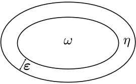
for and set . In this paper we consider kernels such that for
| (2) |
where . Kernels that satisfy (2) are referred to as localized kernels with interaction radius . It is easy to see that for such kernels the interaction domain is a layer of thickness that surrounds , i.e.
see Fig. 1 for a two-dimensional example.
For a symmetric positive definite tensor we respectively define the nonlocal energy semi-norm, nonlocal energy space, and nonlocal volume-constrained energy space by
| (3a) | |||
| (3b) | |||
| (3c) | |||
We also define the volume-trace space , and an associated norm
| (4) |
We refer to [20, 21] for further information about the nonlocal vector calculus.
In order to avoid technicalities not germane to the coupling scheme, in this paper we consider integrable kernels. Examples of applications modeled by the latter can be found in [2, 3, 4]. Specifically, we assume that there exists positive constants and such that
| (5) |
for all . Note that this also implies that there exists a positive constant such that for all
| (6) |
In [20, §4.2] this class of kernels (referred to as Case 2) is rigorously analyzed; we report below an important result, useful throughout the paper.
Lemma 2.1
The latter is a combination of results in Lemmas 4.6 and 4.7 and Corollary 4.8 in [20, §4.3.2]. Note that the lower bound in (7) represents a nonlocal Poincaré inequality. Even though not included in the analysis, singular kernels appear in applications such as peridynamics; numerical results, included in the paper, suggest that the coupling scheme can handle such kernels without difficulties. However, their analysis is beyond the scope of this paper.
2.1 Local-to-Nonlocal coupling setting
Consider a bounded open region with interaction domain . Given and we assume that the volume-constrained333The volume constraint in (8) is the nonlocal analogue of a Dirichlet boundary condition, in which the closed region plays the role of a“boundary”. nonlocal diffusion equation
| (8) |
provides an accurate description of the relevant physical processes in . Let , we assume that the local diffusion model given by the Poisson equation
| (9) |
with suitable boundary data and forcing term is a good approximation of (8) whenever the latter has sufficiently “nice” solutions. In this work we define to be an extension of by in , specifically,
| (10) |
For a symmetric positive definite standard arguments of variational theory show that the weak form444Multiplication of (8) by a test function , integration over and application of the first nonlocal Green’s identity [21] yield the weak form (11) of the nonlocal problem.
| (11) |
of (8) is well-posed [20], i.e., (11) has a unique solution such that
| (12) |
for some positive constant . In this work, for simplicity and without loss of generality, we set .
Although (11) and the nonlocal calculus [20] enable formulation and analysis of finite elements for (8), which parallel those for the Poisson equation (9), resulting methods may be computationally intractable for large domains. The root cause for this is that long-range interactions increase the density of the resulting algebraic system making it more expensive to assemble and solve.
3 Optimization-based LtN formulation
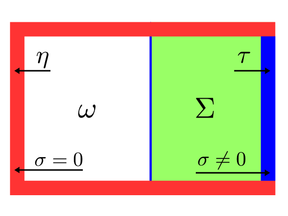
For clarity we consider (8) and (9) with homogeneous Dirichlet conditions on and , respectively. To describe the approach it suffices to examine a coupling scenario where these problems operate on two overlapping subdomains of . Thus we consider partitioning of into a nonlocal subdomain with interaction volume and a local subdomain , with boundary , such that , and ; see Fig. 2.
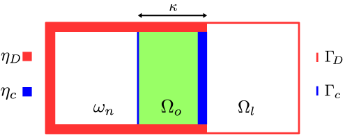
Let , , , and ; see Fig. 2 and Appendix B for a summary of notation and definitions. Restrictions of (8) and (9) to and are given by
| (13) |
respectively, where and are an undetermined Dirichlet volume constraint and an undetermined Dirichlet boundary condition, respectively. The following constrained optimization problem
| (14) |
defines the optimization-based LtN coupling. In this formulation the subdomain problems (13) are the optimization constraints, and are the states and and are the controls. We equip the control space with the norm
| (15) |
In contrast to blending, (14) is an example of a divide-and-conquer strategy as the local and nonlocal problems operate independently in and .
Given an optimal solution of (14) we define the LtN solution by splicing together the optimal states:
| (16) |
We note that there are several ways to define the LtN solution; since our ultimate goal is to approximate a globally nonlocal solution, we set equal to the optimal nonlocal solution over the whole nonlocal domain.
The next section verifies that (14) is well-posed.
3.1 Well-posedeness
We show that for any pair of controls subproblems (13) have unique solutions and , respectively. Elimination of the states from (14) yields the equivalent reduced space form of this problem in terms of and only:
| (17) |
To show that (17) is well-posed we start as in [23, 31] and split, for any given , the solutions of the state equations into a harmonic and a homogeneous part. The harmonic components and of the states solve the equations
| (18) |
respectively. The homogeneous components and solve a similar set of equations but with homogeneous volume constraint and boundary condition, respectively:
| (19) |
In terms of these components , , and the objective
The Euler-Lagrange equation of (17) is given by: seek such that
| (20) |
where and . The following lemma establishes a key property of .
Lemma 3.1
The form defines an inner product on .
Proof. By construction is symmetric and bilinear. Thus, it suffices to show that is positive definite, i.e., if and only if . Let then and , implying . Conversely, if , then in . Let in . Then we have that (i) for all , i.e., is harmonic in , and (ii) for all , i.e., vanishes on a non-empty interior set of . By the identity principle for harmonic functions, in . Because in and on it follows that .
As a results, endows the control space with the “energy” norm
| (21) |
Note that and are continuous with respect to the energy norm. However, the control space may not be complete with respect to the energy norm. In this case, following [1, 17], we consider the optimization problem (17) on the completion of the control space.
Theorem 3.1
Let denote a completion555If is complete, then of course we have that . of the control space with respect to the energy norm (21). Then, the minimization problem
| (22) |
has a unique minimizer such that
| (23) |
Proof. Equation (23) is a necessary condition for any minimizer of (22). Assume first that the control space is complete, i.e. . Then is Hilbert and the projection theorem implies that (23) has a unique solution.
When is not complete, the continuous bilinear form and the continuous functional defined on can be uniquely extended by using the Hahn-Banach theorem to a continuous bilinear form and a continuous functional in . Then, the existence and uniqueness of the minimizer follow as before.
To avoid technical distractions, in what follows we assume that the minimizer belongs to and hence and . We note that in the finite dimensional case the completeness is not an issue, as the discrete control space is Hilbert with respect to the discrete energy norm, see Section 5.
4 Analysis of the LtN coupling error
We define the LtN coupling error as the -norm of the difference between the global nonlocal solution of (8) with homogeneous volume constraints and the LtN solution given by (16). This section shows that the coupling error is bounded by the modeling error on the local subdomain, i.e., the error made by replacing the “true” nonlocal diffusion operator on by the Laplacian.
We prove this result under the following assumptions.
H.2 The global nonlocal solution666This assumption can be relaxed to: has a well-defined trace on . .
We also need the trace operator such that
| (24) |
and the lifting operator , , where
| (25) |
are a harmonic lifting operator and the homogenous part of the states, respectively. Our main result is the following theorem.
Theorem 4.1
Assume that H.1 and H.2 hold. Then, there exists a positive constant such that
where .
For clarity we break the proof of this theorem into several steps arranged in Sections 4.1–4.3. Also for clarity, below we list the ancillary results required for the proof of Theorem 4.1, but to avoid clutter, we collect all their proofs in Appendix A. In what follows we let and , , denote generic positive constants.
Lemma 4.1
[Nonlocal trace inequality] Let where and are an open bounded domain and its associated interaction domain and let , , as in Fig. 7. Assume that is such that . Then
| (26) |
Lemma 4.2
Let , and be defined as in Lemma 4.1. The trace space is a closed subspace of . Furthermore, for all we have that
| (27) |
Application of Lemma 4.2 with and implies that the trace space is a closed subspace of , and thus it is a Hilbert space in the topology. We use this result to prove a strong Cauchy-Schwartz inequality for the nonlocal and local harmonic components of the states, i.e., the solutions to (18). This inequality is essential for the estimate of below.
Lemma 4.3
[Strong Cauchy-Schwartz inequality] There exists such that for all
| (28) |
4.1 The harmonic lifting operator is bounded from above
We prove that is bounded in the operator norm induced by the energy norm (21). We refer to Appendix A for additional notation and auxiliary results used in the proof. We introduce the space .
Lemma 4.4
Assume that H.1 holds. There exists a positive constant such that
| (29) |
where is the thickness of .
Proof. To prove (29) it suffices to show that
for some positive constant , inversely proportional to . According to the definitions of and in (25) and (21), this is equivalent to
where is the indicator function. Since , this inequality reduces to
The strong Cauchy-Schwarz inequality for the harmonic component (see Lemma 4.3) yields the following lower bound for the right hand side:
| (30) | ||||
We now proceed to bound and from below by and , respectively. We start with the nonlocal term. Let denote the extension of by zero in , i.e., in and in . By using the nonlocal Poincaré inequality, the well-posedness of the nonlocal problem and Lemma 4.2 we have
Therefore, we have that
| (31) |
with .
To analyze the local term we derive a Caccioppoli-type inequality for the local harmonic component. We introduce the cutoff function such that in , in , , and , where is the thickness of the overlap, see Fig. 2. These properties imply that and belong to . Next, we note that is the solution of the weak formulation of (9) with . Using as a test function then yields the following identity
We use the latter to find a bound on :
Thus, we conclude that
where is the local Poincaré constant. Let . Together with (30) and (31) this yields
4.2 The approximation error is bounded by the modeling error
The optimal solution of the reduced space problem (17) approximates the trace of the global nonlocal solution on and , respectively. The following lemma shows that the error in is bounded by the modeling error on .
4.3 Proof of Theorem 4.1
Let . Definitions (24) and (25) together with the identities
| (34) |
imply that
| (35) |
Likewise, the identities and imply that . Adding and subtracting to the LtN error then yields
| (36) |
The first term in (36) is the consistency error of ; (35) implies that
| (37) |
To estimate the second term we use (29) and (32):
Combining (36) with this bound and (37) gives
which completes the proof.
4.4 Convergence of the modeling error
In this section we show that vanishes as .
Lemma 4.6
Proof. By definition solves the boundary value problem
and so, it is also a solution of the weak equation
Let solve the dual problem
| (38) |
Since on one can set in (38) to obtain
where the third equality follows from the fact that is extended to zero in and the limit follows from the result in [21, Section 5]777It can be shown that when kernels satisfying (2) and (5) are properly scaled, so that , . The same result holds for the peridynamics kernel in (61)..
Remark 4.1
An immediate consequence of the results in this section is the fact that the LtN solution converges to the corresponding local solution in the limit of vanishing nonlocality. This means that, if an asymptotically-compatible (AC) discretization is used, the discreticretized LtN solution converges to the corresponding continuous local solution as and simultaneously, where is the discretization parameter. In other words, the proposed formulation yields an AC scheme, provided AC discretizations are employed.
5 Approximation of the optimization-based LtN formulation
This section presents the discretization and the error analysis of the LtN formulation (14). Throughout this section we assume that and are polygonal domains; this assumption is not restrictive as those are virtual domains that we can define at our discretion.
5.1 Discretization
We use a reduced-space approach to solve the optimization-based LtN problem (14) numerically, i.e., we discretize and solve the problem
| (39) |
where solves the weak nonlocal equation
| (40) |
for all , and solves the weak local equation
| (41) |
for all . Here, and are the duals of and , respectively.
To discretize (39)–(41) we consider the following conforming finite element spaces [10, 12]
| (42) |
for the nonlocal and local states, controls, and test functions888For simplicity, we approximate , and their duals by the same finite dimensional space., respectively. In general, the finite element spaces for the nonlocal and local problems can be defined on different meshes with parameters and , respectively, and can have different polynomial orders given by integers and , respectively.
Restriction of (39)–(41) to the finite element spaces (42) defines the discrete reduced-space LtN formulation
| (43) |
where solves the discrete nonlocal state equation
| (44) |
and solves the discrete local state equation999Note that both (44) and (45) are well-posed.
| (45) |
Following Section 3.1, we write the solutions of (44) and (45) as
| (46) |
where and are “harmonic” components solving (44) and (45) with and respectively, whereas and are “homogeneous” components solving (44) and (45) with and , respectively. In terms of these components
The Euler-Lagrange equation of (43) has the form: seek such that
| (47) |
where and . To prove the positivity of , the arguments of Lemma 3.1 cannot be extended, as the identity principle does not hold for . We use instead the discrete strong Cauchy-Schwarz inequality in Lemma A.1.
Lemma 5.1
The form defines an inner product on .
Proof. We prove that if and only if . If then and , implying . Conversely, if , then
The discrete strong Cauchy-Schwarz inequality (see Lemma A.1) then implies
| (48) |
Since the left hand side in the above inequality is nonnegative. Thus, we must have that and , which implies .
Lemma A.2 proves that is Hilbert with respect to the discrete energy norm
| (49) |
This fact, Lemma 5.1 and the projection theorem provide the following corollary.
Corollary 5.1
The reduced space problem (43) has a unique minimizer.
5.2 Convergence analysis
In this section we prove that the discrete solution converges to the exact solution assuming the latter belongs to the “raw” control space . This assumption mirrors the one made in [1] and is necessary because the continuous problem is well-posed in the completion of the raw control space. We prove this result under the following assumptions.
H.3 The optimal solution belongs to the raw space: .
H.4 The kernel is translation invariant, i.e. 101010Note that this assumption is not too restrictive; in fact, it is very common in nonlocal mechanics applications..
Let denote the optimal solution of (17) and be the optimal solution of its discretization (43). We denote the associated optimal states by , and , respectively, that is,
We will estimate the discrete energy norm of the error using Strang’s second111111The discrete problem (47) also fits in the setting of Strang’s first Lemma [22, Lemma 2.27, p.95]. We use the second lemma because it simplifies the analysis. Lemma; see, e.g., [22, Lemma 2.25, p.94]. Application of this lemma is contingent upon two conditions: (i) the discrete form is continuous and coercive with respect to , and (ii) there exists a positive real constant such that
| (50) |
The first assumption holds trivially. To verify (50) note that
Given the function solves the weak equation
where is the projection onto , i.e., . Similarly, we have that , where is the projection onto . Additionally, similarly to [1], we assume that there exist positive constants , , , and such that for and small enough the following inequalities hold:
| (51) | |||||
The latter, the strong Cauchy-Schwarz inequality and the boundedness of the projection operators yield
| (52) | ||||
Application of Strang’s second lemma then yields the following error estimate.
We use the result in Lemma 5.2 to obtain asymptotic convergence rates under the assumption that 1) the homogeneous problems (19) have solutions , for , and ; 2) the control variables are such that and . We treat the first term in (53) by using the norm-equivalence (67); we have
| (54) | ||||
where is defined as in (15). We focus on the second term in (53). Adding and subtracting and using conformity of gives
Adding and subtracting the terms
to the last expression and using the definitions of , , and yields the identity:
Application of the Cauchy-Schwartz inequality then gives the following upper bound:
Furthermore, note that , and that is the optimal value of the objective functional, which is bounded by the modeling error. The regularity assumptions on the nonlocal solutions in (19) allow us to apply Theorem 6.2 in [20, p.689]:
where . Furthermore, the regularity assumptions on the local solutions in (19) allow us to use Corollary 1.122 in [22, p.66] to conclude that
According to Weyl’s Lemma [35] the local harmonic liftings and are smooth functions and so there are positive constants and such that
While a similar result holds for the nonlocal harmonic lifting , the treatment of is more involved, due to the discrete nature of the Dirichlet data, and it requires an auxiliary function such that , for an arbitrarily small . Because and depend continuously on the data,
| (55) | ||||
Since can be arbitrarily small, the last two terms in (55) are negligible. To complete the estimate we only need a uniform bound on . To this end, assume that for all , with . Under this assumption for all . Taking into account that is nonlocal harmonic, i.e., , it follows that , i.e., is also nonlocal harmonic for all . Thus, has a uniformly bounded norm, i.e. . This implies the existence of a positive constant such that, . It follows that there exist positive constants and such that
We have just shown the following result.
Theorem 5.1
Assume that H.1–H.4 hold. Then, there exist positive constants such that
| (56) |
We use Theorem 5.1 to estimate the norm of the discretization error.
Corollary 5.2
Assume that H.1–H.4 hold. Then, there exist positive constants such that
| (57) |
6 Numerical tests
We present numerical tests with the new LtN formulation in one dimension, including a patch test, a convergence study and approximation of discontinuous solutions. Though preliminary, these results show the effectiveness of the coupling method, illustrate the theoretical results, and provide the basis for realistic simulations. In our examples we use an integrable kernel, , satisfying assumptions (2) and (5) to illustrate theoretical results and a singular kernel, , often used in the literature as an approximation of a peridynamic model for nonlocal mechanics. These kernels are given by
| (61) |
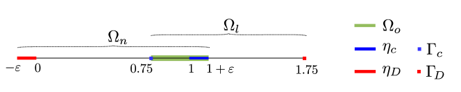
respectively. Even though does not satisfy our theoretical assumptions121212The energy space associated with is not equivalent to a Sobolev space, nevertheless it is a separable Hilbert space whose energy norm satisfies a nonlocal Poincaré inequality., these numerical results demonstrate the effectiveness of the LtN coupling for realistic, practically important, nonlocal models. In all examples we consider the LtN problem configuration shown in Fig. 3, where , , , , , , and .
In all numerical tests , , and are discontinuous piecewise linear finite element spaces, while and are piecewise linear finite elements. We use the same grid size for the local and nonlocal finite element spaces. To solve the LtN optimization problem we apply the gradient based Quasi-Newton scheme BFGS [30].
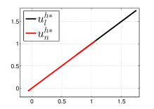
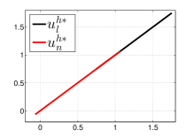
The patch test
This test uses the linear manufactured solution , , , . We expect the LtN formulation to recover this solution exactly, i.e., and . Figure 4 shows the optimal states and , computed with and , for (left) and (right). The LtN method recovers the exact solution to machine precision.
 |
 |
Convergence tests
We examine the convergence of finite element approximations with respect to the grid size using the following manufactured solutions:
- M.1
-
, , , .
- M.2
-
, , , .
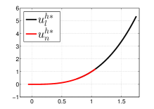
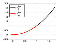
Note that, for both kernels, the associated nonlocal operator is equavalent to the classical Laplacian for polynomials up to the third order. For examples M.1 and M.2 we compute the convergence rates and the norm of the errors for the nonlocal state, , the local state, , and the nonlocal control parameter, . The results are reported in Tables 1 and 2 for and in Tables 3 and 4 for in correspondence of different values of interaction radius and grid size . In Fig. 5 we also report the optimal discrete solutions.
Results in Tables 1 and 2 show optimal convergence for state and control variables. We note that according to [20] and FE convergence theory [22] this is the same rate as for the independent discretization of the nonlocal and local equations by piecewise linear elements.
Remark 6.1
The convergence analysis in Section 5.2 establishes a suboptimal convergence rate in the norm of the discretization error of the state variables as we lose half order of convergence. We believe that the bound in (60) is not sharp, in fact, additional numerical tests (with ) show that there is no convergence deterioration.
For the singular kernel there are no theoretical convergence results; however, there is numerical evidence that piecewise linear approximations of (11) are second-order accurate; see [6]. Our numerical experiments in Tables 3 and 4 show that the optimization-based LtN solution converges at the same rate.
 |
 |
|
 |
| rate | rate | rate | |||||
|---|---|---|---|---|---|---|---|
| 2.63e-03 | - | 2.76e-03 | - | 5.59e-05 | - | ||
| 6.16e-04 | 2.10 | 6.74e-04 | 2.04 | 2.63e-05 | 1.09 | ||
| 0.010 | 1.40e-04 | 2.13 | 1.63e-04 | 2.05 | 1.14e-05 | 1.20 | |
| 3.46e-05 | 2.02 | 4.04e-05 | 2.01 | 4.18e-06 | 1.47 | ||
| 2.24e-03 | - | 2.56e-03 | - | 6.34e-04 | - | ||
| 7.56e-04 | 1.56 | 7.13e-04 | 1.85 | 1.78e-04 | 1.83 | ||
| 0.065 | 1.89e-04 | 2.00 | 1.78e-04 | 2.00 | 4.46e-05 | 2.00 | |
| 4.73e-05 | 2.00 | 4.46e-05 | 2.00 | 1.12e-05 | 2.00 | ||
| 1.18e-05 | 2.00 | 1.11e-05 | 2.00 | 2.82e-06 | 1.99 |
| rate | rate | rate | |||||
|---|---|---|---|---|---|---|---|
| 4.89e-03 | - | 1.09e-02 | - | 2.04e-04 | - | ||
| 1.23e-03 | 1.99 | 2.74e-03 | 2.00 | 9.63e-05 | 1.08 | ||
| 0.010 | 3.11e-04 | 1.99 | 6.86e-04 | 2.00 | 4.16e-05 | 1.21 | |
| 7.85e-05 | 1.99 | 1.72e-04 | 2.00 | 1.45e-05 | 1.51 | ||
| 1.95e-05 | 2.01 | 4.29e-05 | 2.00 | 3.16e-06 | 2.20 | ||
| 5.41e-03 | - | 1.09e-02 | - | 2.29e-03 | - | ||
| 1.34e-03 | 2.01 | 2.74e-03 | 2.00 | 5.46e-04 | 2.07 | ||
| 0.065 | 3.38e-04 | 1.99 | 6.86e-04 | 2.00 | 1.38e-04 | 1.99 | |
| 8.46e-05 | 2.00 | 1.71e-04 | 2.00 | 3.46e-05 | 1.99 | ||
| 2.12e-05 | 2.00 | 4.29e-05 | 2.00 | 8.73e-06 | 1.99 |
| rate | rate | rate | |||||
|---|---|---|---|---|---|---|---|
| 2.67e-03 | - | 2.78e-03 | - | 5.79e-05 | - | ||
| 6.33e-04 | 2.08 | 6.81e-04 | 2.03 | 2.72e-05 | 1.09 | ||
| 0.010 | 1.47e-04 | 2.11 | 1.65e-04 | 2.04 | 1.19e-05 | 1.20 | |
| 3.63e-05 | 2.01 | 4.11e-05 | 2.01 | 4.29e-06 | 1.47 | ||
| 9.10e-06 | 2.00 | 1.03e-05 | 2.00 | 1.05e-06 | 2.03 | ||
| 2.36e-03 | - | 2.62e-03 | - | 6.52e-04 | - | ||
| 7.54e-04 | 1.65 | 7.12e-04 | 1.88 | 1.78e-04 | 1.87 | ||
| 0.065 | 1.88e-04 | 2.00 | 1.78e-04 | 2.00 | 4.45e-05 | 2.00 | |
| 4.67e-05 | 2.01 | 4.44e-05 | 2.00 | 1.11e-05 | 2.00 | ||
| 1.14e-05 | 2.04 | 1.10e-05 | 2.01 | 2.76e-06 | 2.01 |
| rate | rate | rate | |||||
|---|---|---|---|---|---|---|---|
| 4.90e-03 | - | 1.09e-02 | - | 2.07e-04 | - | ||
| 1.23e-03 | 1.99 | 2.74e-03 | 2.00 | 9.68e-05 | 1.10 | ||
| 0.010 | 3.11e-04 | 1.99 | 6.86e-04 | 2.00 | 4.17e-05 | 1.21 | |
| 7.85e-05 | 1.99 | 1.72e-04 | 2.00 | 1.46e-05 | 1.52 | ||
| 1.96e-05 | 2.01 | 4.29e-05 | 2.00 | 3.17e-06 | 2.00 | ||
| 5.40e-03 | - | 1.09e-02 | - | 2.31e-03 | - | ||
| 1.34e-03 | 2.01 | 2.74e-03 | 2.00 | 5.46e-04 | 2.08 | ||
| 0.065 | 3.37e-04 | 1.99 | 6.86e-04 | 2.00 | 1.38e-04 | 2.00 | |
| 8.46e-05 | 2.00 | 1.72e-04 | 2.00 | 3.46e-05 | 1.99 | ||
| 2.12e-05 | 2.00 | 4.29e-05 | 2.00 | 8.73e-06 | 1.99 |
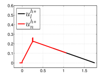
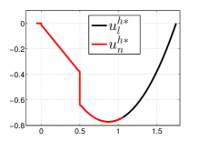
Recovery of singular features
The tests in this section are motivated by nonlocal mechanics applications and demonstrate the effectiveness of the coupling method in the presence of point forces and discontinuities. We use the following two manufactured solution examples:
- A.1
-
, , , being the Dirac function.
- A.2
-
, ,
In Fig. 6 we report the optimal discrete solutions for and . In particular, A.2 is a significant example that shows the usefulness of the coupling method in approximating the true solution with a local model where the nonlocality effects are not pronounced, i.e. the solution is smooth.
 |
 |
Acknowledgements
This work was supported by the Sandia National Laboratories (SNL) Laboratory-directed Research and Development (LDRD) program, and the U.S. Department of Energy, Office of Science, Office of Advanced Scientific Computing Research under Award Number DE-SC-0000230927 and under the Collaboratory on Mathematics and Physics-Informed Learning Machines for Multiscale and Multiphysics Problems (PhILMs) project. Sandia National Laboratories is a multimission laboratory managed and operated by National Technology and Engineering Solutions of Sandia, LLC., a wholly owned subsidiary of Honeywell International, Inc., for the U.S. Department of Energys National Nuclear Security Administration contract number DE-NA0003525. This paper describes objective technical results and analysis. Any subjective views or opinions that might be expressed in the paper do not necessarily represent the views of the U.S. Department of Energy or the United States Government. Report Number: SAND2019-12937.
Appendix A Ancillary results
This appendix contains proofs of several results necessary for the estimate of and additional results necessary for the well-posedness of the discrete reduced space problem. We recall that in the following proofs and , , are generic positive constants.
Proof of Lemma 4.1. We need the following subspaces of and
| (62) |
Let be the indicator of . Definition (4) and the fact that vanishes on imply that
To bound the energy norm of note that
where the last two inequalities follow from (6) and (7) respectively. Thus,
with .
Proof of Lemma 4.2. Consider a sequence such that in . To show that consider the function such that and . To complete the proof it remains to show that has finite energy norm. Using the norm equivalence in Lemma 2.1
Therefore, and , hence . Finally, let be such that ; by Lemmas 4.1 and 2.1, .
Proof of Lemma 4.3. We prove (28) by contradiction. If (28) does not hold then for all , there exist such that the corresponding harmonic components and satisfy and and
| (63) |
Note that
This implies that the sequence of inner products converges, i.e. . Furthermore, since and are bounded, there exist subsequences, still denoted by and , such that
| (64) |
Since is compactly embedded in , we also have
| (65) |
The weak convergence of the sequences also implies that and . Properties (64) and (65) then imply that
where the last inequality follows from the strong convergence of the local component:
Thus,
This means that . This identity holds if and only if for some real . To complete the proof we apply the same argument as in Lemma 3.1. On the one hand in and so, in . On the other hand, is harmonic in and the identity principle implies that in . Thus, (63) holds if and only if in , a contradiction.
Next, we prove two results that are necessary for the analysis conducted in Section 5.
Lemma A.1
Proof. In this proof we follow the same arguments of Lemma A.7 of [1].
Let be a sequence of mesh sizes for the nonlocal and local finite element approximations such that as . Also, let and be the nonlocal and local discrete harmonic components corresponding to and . It is well-known [22] that the local finite element solution converges strongly in to the infinite-dimensional solution as . Furthermore, paper [20] shows that when is such that (5) holds the nonlocal finite element solution converges strongly in the energy norm to the infinite-dimensional solution . Due to the Poincaré inequality such convergence implies the storng convergence in the norm. Thus, we have
Since the strong convergence in implies the weak convergence and the convergence in norm, the following are also true
Using the strong Cauchy-Schwarz inequality (28), we obtain
Thus, such that , such that
Lemma A.2
The space is Hilbert with respect to the inner product .
Proof. By assumption is a closed subspace . Thus, it is Hilbert with respect to . Let ; we show that and are equivalent, i.e. there exist and such that
| (67) |
Using the well-posedness of the discrete problems, we have
On the other hand, we have
| Local trace inequality | ||||
| Local inverse inequality [7] | ||||
| Strong Cauchy-Schwarz | ||||
Choosing and , we obtain (67).
Appendix B Notation summary
In this appendix we report a summary of the notation we use for local and nonlocal domains. In Table 5 we report local entities on the left and nonlocal entities on the right (see Fig. 2 for a two-dimensional configuration).
| Symbol | Definition | Symbol | Definition |
| interior of | |||
| interaction domain of | |||
| local subdomain | nonlocal subdomain, | ||
| interior of | |||
| interaction domain of | |||
| overlap domain, | |||
References
- [1] A. Abdulle, O. Jecker, and A. Shapeev. An optimization based coupling method for multiscale problems. Technical Report 36.2015, EPFL, Mathematics Institute of Computational Science and Engineering, Lausanne, Switzerland, December 2015.
- [2] B. Aksoylu and T. Mengesha. Results on nonlocal boundary value problems. Numerical Functional Analysis and Optimization, 31(12):1301–1317, 2010.
- [3] B. Aksoylu and M. L. Parks. Variational theory and domain decomposition for nonlocal problems. Applied Mathematics and Computation, 217(14):6498 – 6515, 2011.
- [4] F. Andreu-Vaillo, J.M. Mazón, J.D. Rossi, and J.J. Toledo-Melero. Nonlocal diffusion problems. American Mathematical Society ; Real Sociedad Matemática Española, 2010.
- [5] Y. Azdoud, F. Han, and G. Lubineau. A morphing framework to couple non-local and local anisotropic continua. International Journal of Solids and Structures, 50(9):1332 – 1341, 2013.
- [6] X. Chen and M. D. Gunzburger. Continuous and discontinuous finite element methods for a peridynamics model of mechanics. Computer Methods in Applied Mechanics and Engineering, 200(9–12):1237 – 1250, 2011.
- [7] P. Ciarlet. The Finite Element Method for Elliptic Problems. SIAM Classics in Applied Mathematics. SIAM, Philadelphia, 2002.
- [8] M. D’Elia and P. Bochev. Optimization-based coupling of nonlocal and local diffusion models. In R. Lipton, editor, Proceedings of the Fall 2014 Materials Research Society Meeting, MRS Symposium Proceedings, Boston, MA, November 2014. Cambridge University Press.
- [9] M. D’Elia, P. Bochev, D. Littlewood and M. Perego. Optimization-based coupling of local and nonlocal models: Applications to peridynamics. in Handbook of Peridynamic Modeling, (19), Modern Mechanics and Mathematics. Taylor & Francis, 2015.
- [10] M. D’Elia, Q. Du, C. Glusa, M. D. Gunzburger, X. Tian, and Z. Zhou. Numerical methods for nonlocal and fractional models. Acta Numerica, to appear, 2020.
- [11] M. D’Elia, Q. Du, M. D. Gunzburger, and R. B. Lehoucq. Finite range jump processes and volume–constrained diffusion problems. Computational Methods in Applied Mathematics, (29), 2017.
- [12] M. D’Elia, M. Gunzburger, and C. Vollmann. A cookbook for finite element methods for nonlocal problems, including quadrature rules and approximate Euclidean balls. arXiv:2005.10775, 2020.
- [13] M. D’Elia, X. Li, P. Seleson, X. Tian, Y. Yu. A review of Local-to-Nonlocal coupling methods in nonlocal diffusion and nonlocal mechanics. Journal of Peridynamics and Nonlocal Modeling, to appear, 2020.
- [14] M. D’Elia, M. Perego, P. Bochev, and D. Littlewood. A coupling strategy for nonlocal and local diffusion models with mixed volume constraints and boundary conditions. Computers & Mathematics with Applications, 71(11):2218 – 2230, 2016. Proceedings of the conference on Advances in Scientific Computing and Applied Mathematics. A special issue in honor of Max Gunzburger’s 70th birthday.
- [15] H. B. Dhia and G. Rateau. The Arlequin method as a flexible engineering design tool. International Journal for Numerical Methods in Engineering, 62(11):1442–1462, 2005.
- [16] M. Di Paola, G. Failla, and M. Zingales. Physically-based approach to the mechanics of strong non-local linear elasticity theory. Journal of Elasticity, 97(2):103–130, 2009.
- [17] M. Discacciati, P. Gervasio, and A. Quarteroni. The interface control domain decomposition (icdd) method for elliptic problems. SIAM Journal on Control and Optimization, 51(5):3434–3458, 2013.
- [18] Q. Du. Optimization based nonoverlapping domain decomposition algorithms and their convergence. SIAM Journal on Numerical Analysis, 39(3):1056–1077, 2001.
- [19] Q. Du and M. D. Gunzburger. A gradient method approach to optimization-based multidisciplinary simulations and nonoverlapping domain decomposition algorithms. SIAM Journal on Numerical Analysis, 37(5):pp. 1513–1541, 2000.
- [20] Q. Du, M. D. Gunzburger, R. B. Lehoucq, and K. Zhou. Analysis and approximation of nonlocal diffusion problems with volume constraints. SIAM Review, 54(4):667–696, 2012.
- [21] Q. Du, M. D. Gunzburger, R. B. Lehoucq, and K. Zhou. A nonlocal vector calculus, nonlocal volume-constrained problems and nonlocal balance lows. Mathematical Models and Methods in Applied Sciences, 23(03):493–540, 2013.
- [22] A. Ern and J.-L. Guermond. Theory and Practice of Finite Elements. Number 159 in Applied Mathematical Sciences. Springer Verlag, New York, 2004.
- [23] P. Gervasio, J.-L. Lions, and A. Quarteroni. Heterogeneous coupling by virtual control methods. Numerische Mathematik, 90:241–264, 2001. 10.1007/s002110100303.
- [24] M. D. Gunzburger, M. Heinkenschloss, and H. K. Lee. Solution of elliptic partial differential equations by an optimization-based domain decomposition method. Applied Mathematics and Computation, 113(2-3):111 – 139, 2000.
- [25] M. D. Gunzburger and H. K. Lee. An optimization-based domain decomposition method for the Navier-Stokes equations. SIAM Journal on Numerical Analysis, 37(5):pp. 1455–1480, 2000.
- [26] M. D. Gunzburger, J. S. Peterson, and H. Kwon. An optimization based domain decomposition method for partial differential equations. Computers & Mathematics with Applications, 37(10):77 – 93, 1999.
- [27] F. Han and G. Lubineau. Coupling of nonlocal and local continuum models by the Arlequin approach. International Journal for Numerical Methods in Engineering, 89(6):671–685, 2012.
- [28] P. Kuberry and H. Lee. A decoupling algorithm for fluid-structure interaction problems based on optimization. Computer Methods in Applied Mechanics and Engineering, 2013.
- [29] G. Lubineau, Y. Azdoud, F. Han, C. Rey, and A. Askari. A morphing strategy to couple non-local to local continuum mechanics. Journal of the Mechanics and Physics of Solids, 60(6):1088 – 1102, 2012.
- [30] J. Nocedal and S. Wright. Numerical Optimization. Springer Verlag, New York, 1999.
- [31] D. Olson, P. Bochev, M. Luskin, and A. Shapeev. An optimization-based atomistic-to-continuum coupling method. SIAM Journal on Numerical Analysis, 52(4):2183–2204, 2014.
- [32] D. Olson, P. Bochev, M. Luskin, and A. V. Shapeev. Development of an optimization-based atomistic-to-continuum coupling method. In Ivan Lirkov, Svetozar Margenov, and Jerzy Waśniewski, editors, Large-Scale Scientific Computing, volume 8353 of Lecture Notes in Computer Science, pages 33–44. Springer Berlin Heidelberg, 2014.
- [33] P. Seleson, S. Beneddine, and S. Prudhomme. A force-based coupling scheme for peridynamics and classical elasticity. Computational Materials Science, 66:34–49, 2013.
- [34] S. A. Silling and R. B. Lehoucq. Peridynamic theory of solid mechanics. volume 44 of Advances in Applied Mechanics, pages 73 – 168. Elsevier, 2010.
- [35] H. Weyl. The method of orthogonal projection in potential theory. Duke Math. J., 7(1):411–444, 1940.