The global indicator of classicality of an arbitrary $\boldsymbol{N}$-level quantum system

Abstract

It is commonly accepted that a deviation of the Wigner quasiprobability distribution of a quantum state from a proper statistical distribution signifies its nonclassicality. Following this ideology, we introduce the global indicator $\mathcal{Q}_{N}$ for quantification of “classicality-quantumness” correspondence in the form of the functional on the orbit space $\mathcal{O}[\mathfrak{P}_{N}]$ of the $SU(N)$ group adjoint action on the state space $\mathfrak{P}_{N}$ of an $N$-dimensional quantum system. The indicator $\mathcal{Q}_{N}$ is defined as a relative volume of a subspace $\mathcal{O}[\mathfrak{P}^{(+)}_{N}]\subset\mathcal{O}[\mathfrak{P}_{N}]\,,$ where the Wigner quasiprobability distribution is positive. An algebraic structure of $\mathcal{O}[\mathfrak{P}^{(+)}_{N}]$ is revealed and exemplified by a single qubit $(N=2)$ and single qutrit $(N=3)$. For the Hilbert-Schmidt ensemble of qutrits the dependence of global indicator on the moduli parameter of the Wigner quasiprobability distribution has been found.

1 Introduction

Over the past decades, a number of witnesses and measures of nonclassicality of quantum systems have been formulated (see e.g. [1, 2, 3]). Most of them are based on the primary impossibility of a classical statistical description of quantum systems. Particularly, the non-existence of positive definite probability distributions serves as a certain indication of nonclassicality of a physical system.

In the present note, we will focus on the problem of quantifying the nonclassicality of quantum systems associated with a finite-dimensional Hilbert space by studying the non-positivity of the Wigner quasiprobability distributions (the Wigner function, or shortly WF) [6, 7, 8, 9]. Our treatment is based on the recent publications [10, 11], where the Wigner quasiprobability distribution $W^{(\boldsymbol{\nu})}_{\varrho}(\Omega_{N})$ of an $N\--$level quantum system is constructed via the dual pairing,

$$W^{(\boldsymbol{\nu})}_{\varrho}(\Omega_{N})=\mbox{tr}\left[\varrho\,\Delta(\Omega_{N}\,|\,\boldsymbol{\nu})\right]\,,$$ (1)

of the density matrix $\varrho$ – an element of a quantum state space $\mathfrak{P}_{N}$:

$$\mathfrak{P}_{N}=\{X\in M_{N}(\mathbb{C})\ |\ X=X^{\dagger}\,,\quad X\geq 0\,,\quad\mbox{tr}\left(X\right)=1\}\,,$$ (2)

and an element of dual space $\Delta(\Omega_{N}\,|\,\boldsymbol{\nu})\in\mathfrak{P}^{\ast}_{N}\,$– the so-called Stratonovich-Weyl (SW) kernel. The dual space $\mathfrak{P}^{\ast}_{N}$ is defined as:

$$\mathfrak{P}^{\ast}_{N}=\{X\in M_{N}(\mathbb{C})\ |\ X=X^{\dagger}\,,\quad\mbox{tr}\left(X\right)=1\,,\quad\mbox{tr}\left(X^{2}\right)=N\}\,,$$ (3)

and SW kernel is a mapping between phase space $\Omega_{N}$ and dual space $\mathfrak{P}^{\ast}_{N}\,.$ Assuming that SW kernel $\Delta(\Omega_{N})\,$ has the isotropy group $H\in U(N)$ of the form

$$H={U(k_{1})\times U(k_{2})\times U(k_{s+1})}\,,$$

we identify phase-space $\Omega_{N}$  as a complex flag manifold,

$$\Omega_{N}\,\to\,\mathbb{F}^{N}_{d_{1},d_{2},\dots,d_{s}}={U(N)}/{H}\,,$$

where $(d_{1},d_{2},\dots,d_{s})$ is a sequence of positive integers with sum $N$, such that $k_{1}=d_{1}$ and $k_{i+1}=d_{i+1}-d_{i}$ with $d_{s+1}=N\,.$

The Wigner function defined in eqs. (1) - (3) possesses all the properties of a proper statistical distribution except for the non-negativity of the latter. From a physical point of view, the positiveness of probability distributions is a fundamental element of the classical statistical paradigm. Therefore, if WF attains negative values, it is undeniable that a physical system shows some “nonclassical” behaviour. Following this observation, we introduce the global indicator of classicality $\mathcal{Q}_{N}$ characterizing the degree of closeness of a quasiprobability distribution to a proper one. Commonly used measures of deviation from classicality are defined as functionals either on a quantum state space (the measures based on the distance from the base “classical state”), or on phase space (the measures which depend on the volume of a phase space region where WF is negative [2]). In contrast to this approach, we follow an alternative one, the so-called “minimal description” when characteristics of quantum systems are given exceptionally in the terms of $SU(N)\--$invariants. In other words, we intend to define the global indicator $\mathcal{Q}_{N}$ as a functional over the unitary orbit space $\mathcal{O}[\mathfrak{P}_{N}]$. With this aim, let us introduce:

1. Definition 1 The unitary orbit space $\mathcal{O}[\mathfrak{P}_{N}]$ is the quotient space under the equivalence relation imposed by the adjoint $SU(N)$ action on the state space $\mathfrak{P}_{N}$ with quotient (canonical) mapping:

   $$\pi:\ \mathfrak{P}_{N}\longrightarrow\mathcal{O}[\mathfrak{P}_{N}]={\mathfrak{P}_{N}}/{SU(N)}\,;$$ (4)

2. Definition 2 The subset $\Omega^{(+)}_{N}[\varrho]$ of phase space $\Omega_{N}\,,$ where the Wigner function of a given state $\varrho$ is non-negative, is

   $$\Omega^{(+)}_{N}[\varrho]=\{\,x\in\Omega_{N}\,\ |\ W_{\varrho}(\Omega_{N})\geq 0\,\,\}\,;$$ (5)

3. Definition 3 The subspace $\mathfrak{P}_{N}^{(+)}\subset\mathfrak{P}_{N}$ is composed from states $\varrho$ so that

   $$\mathfrak{P}^{(+)}_{N}=\{\varrho\in\mathfrak{P}_{N}\,\ |\ \Omega^{(+)}_{N}[\varrho]=\Omega_{N}\,\ \};$$ (6)

4. Definition 4 The subset $\mathcal{O}[\mathfrak{P}^{(+)}_{N}]$ represents the image of $\mathfrak{P}_{N}^{(+)}$ under the quotient mapping (4):

   $$\mathcal{O}[\mathfrak{P}^{(+)}_{N}]=\pi[\mathfrak{P}_{N}^{(+)}]=\{\pi(x)\,\ |\ x\in\mathfrak{P}_{N}^{(+)}\,\}\,.$$ (7)

Using the definitions above, we introduce the global indicator of nonclassicality $\mathcal{Q}_{N}$ of an N-dimensional quantum system as the following ratio:

$$\mathcal{Q}_{N}=\frac{\mbox{Volume of orbit subspace}\ \mathcal{O}[\mathfrak{P}_{N}^{(+)}]}{\mbox{Volume of orbit space}\ \mathcal{O}[\mathfrak{P}_{N}]}\,.$$ (8)

In order to make this definition self-consistent, we assume that:

• $\mathcal{O}[\mathfrak{P}_{N}]\,,\Omega^{(+)}_{N}[\varrho]\,,\mathfrak{P}_{N}^{(+)}]\,$ and $\mathcal{O}[\mathfrak{P}_{N}^{(+)}]$ are open, connected sets of $\mathbb{R}^{n}$ ;

• The volume of the orbit space in (8) is associated with a measure induced by the quotient mapping $\pi$ from certain Riemannian metric on $\mathfrak{P}_{N}$ .

In order to perform efficient computations of $\mathcal{Q}_{N}$ , it is necessary to have, instead of implicit definitions (6) and (7), a more constructive representation of the space $\mathcal{O}[\mathfrak{P}_{N}^{(+)}]\,.$ With this aim we remind some facts on the stratified structure of state space $\mathfrak{P}_{N}\,.$ First of all, note that $U(N)$ automorphism of the Hilbert space of an $N\--$level quantum system induces the adjoint $SU(N)$ action on the state space:

$$g\cdot\varrho=g\varrho g^{\dagger}\,,\qquad g\in SU(N)\,.$$ (9)

The group action (9) sets an equivalence relations between elements of $\mathfrak{P}_{N}\,$ and gives rise to $SU(N)$ orbit classification. Formally, a subgroup $H_{x}\subset SU(N)$ is the isotropy group (stabilizer) of a point $x\in\mathfrak{P}_{N}\,,$

$$H_{x}=\{g\in SU(N)\ |\ g\cdot x=x\}\,,$$

and points $x,y\in\mathfrak{P}_{N}$ are said to be of the same type if their stabilizers $H_{x}$ and $H_{y}$ are conjugate subgroups of $SU(N)$ group. The orbit type of the point $x\in\mathfrak{P}_{N}$ is given by the conjugacy class of the corresponding isotropy group $[H_{x}]\,.$ Up to conjugation in $SU(N)$ , the isotropy groups $H_{x}$ are in one-to-one correspondence with the Young diagrams corresponding to a possible decomposition of $N$ into non-negative integers. Hence, for given $N$ for any $[H_{\alpha}]\,,\ \alpha=1,2,\dots,P(N)$ one can associate the stratum $\mathfrak{P}_{[H_{\alpha}]}\,,$ defined as the set of all points of $\mathfrak{P}_{N}$ whose stabilizer is conjugate to $H_{\alpha}$:

$$\mathfrak{P}_{[H_{\alpha}]}:=\big{\{}x\in\ \mathfrak{P}_{N}|\ H_{x}\mbox{~{}is~{}conjugate~{}to}\ H_{\alpha}\big{\}}\,.$$ (10)

The union of sets $\mathfrak{P}_{[H_{\alpha}]}$ gives the decomposition of state space $\mathfrak{P}_{N}$ into orbit types

$$\mathfrak{P}_{N}=\bigcup_{\mbox{orbit types}}{\mathfrak{P}}_{[H_{\alpha}]}\,.$$ (11)

Having in mind the above notions and argumentation, we can formulate the following assertion.

$\bullet$ Proposition I $\bullet$  Let $\boldsymbol{r}^{\downarrow}=\{r_{1},r_{2},\dots,r_{N}\}$ and $\boldsymbol{\pi}^{\uparrow}=\{\pi_{N},\pi_{N-1},\dots,\pi_{1}\}$ be eigenvalues of a density matrix $\varrho$ and SW kernel $\Delta(\Omega_{N}\,|\,\boldsymbol{\nu})\,,$ arranged in decreasing and increasing orders respectively. Then,

• The Wigner function $W_{\varrho}(\boldsymbol{\theta})$ of any state $\varrho\in\mathfrak{P}_{N}$ is bounded and there exist $\boldsymbol{\theta}_{-}\,,\boldsymbol{\theta}_{+}\in\Omega_{N}$ such that

  $$W_{\varrho}(\boldsymbol{\theta}_{-})=\inf_{\boldsymbol{\theta}\in\Omega_{N}}\,W_{\varrho}(\boldsymbol{\theta})\,,\qquad W_{\varrho}(\boldsymbol{\theta}_{+})=\sup_{\boldsymbol{\theta}\in\Omega_{N}}\,W_{\varrho}(\boldsymbol{\theta})\,;$$

• If $\varrho_{1},\varrho_{2}\in\mathfrak{P}_{[H_{\alpha}]}\,,$ then extreme values of the corresponding Wigner functions are related as follows,

  $$\inf_{\boldsymbol{\theta}}\,W_{\varrho_{1}}(\boldsymbol{\theta})=\inf_{\boldsymbol{\theta}}\,W_{\varrho_{2}}(\boldsymbol{\theta})\,,\qquad\sup_{\boldsymbol{\theta}}\,W_{\varrho_{1}}(\boldsymbol{\theta})=\sup_{\boldsymbol{\theta}}\,W_{\varrho_{2}}(\boldsymbol{\theta})\,;$$ (12)

• $\mathcal{O}[\mathfrak{P}_{N}^{(+)}]\,$ can be identified as a dual cone of a subset $\mathcal{O}[\mathfrak{P}_{N}]\subset\mathbb{R}^{N-1}$:

  $$\mathcal{O}[\mathfrak{P}_{N}^{(+)}]=\ \left\{\,\boldsymbol{\pi}\in\mathcal{O}[\mathfrak{P}^{\ast}_{N}]\ \,|\ \,(\boldsymbol{r}^{\downarrow},\boldsymbol{\pi}^{\uparrow})\geq 0,\quad\forall\,\boldsymbol{r}\in\mathcal{O}[\mathfrak{P}_{N}]\,\right\}\,,$$ (13)

  where the dual pairing $(\,,\,)$ in (13) is

  $$(\boldsymbol{r}^{\downarrow},\boldsymbol{\pi}^{\uparrow})=r_{1}\pi_{N}+r_{2}\pi_{N-1}+\dots+r_{N}\pi_{1}\,.$$ (14)

The correctness of the above proposition stems from the following observations. At first, according to our construction, an $N\--$level system is associated with a symplectic manifold $\Omega_{N}\,,$ which is compact. Secondly, the Wigner distributions of trace-class operators are continuous functions (cf. discussion in [13]. Hence, in accordance to the multivariable Weierstrass extreme value theorem, the Wigner function attains its extreme values on the $\Omega_{N}$. Moreover, the absolute maximum and minimum must occur at a critical point of WF in $\Omega_{N}$ or at a boundary point of $\Omega_{N}$. Some technical details of the proof of Proposition I are given in the Appendix.

The article is organized as follows. The next section is devoted to a brief exposition of necessary facts about WF of finite-dimensional systems mainly borrowed from our recent articles [10, 11]. In Section 3. we present a reinterpretation of the Wigner distributions as a functions defined over the space of the unistochastic matrices and describe their continuation to the whole Birkhoff polytope. With the aid of this extension, the global extrema of WF is derived. In Section 4., using the lower and upper bounds for WF the orbit subspace $\mathcal{O}[\mathfrak{P}^{(+)}_{N}]\,,$ the global $\mathcal{Q}\--$indicators for $N=2$ (qubit) and $N=3$ are obtained. Final remarks are collected in Section 5.

2 Basic settings

$\bullet$ Wigner function of $N$-level system $\bullet$  A density matrix $\varrho$ and Stratonovich-Weyl kernel $\Delta(\Omega_{N}\,|\,\boldsymbol{\nu})$ obey the following decompositions into the Lie algebra $\mathfrak{su}(N)$ and its dual $\mathfrak{su}(N)^{*}$,

$$\varrho = \frac{1}{N}\mathbb{I}_{N}+\frac{1}{N}\,\imath\,\mathfrak{su}(N)\,,$$ (15)

$$\Delta(\Omega_{N}\,|\,\boldsymbol{\nu}) = \frac{1}{N}\mathbb{I}_{N}+\kappa\,\frac{1}{N}\,\imath\,\mathfrak{su}(N)^{\ast}\,,$$ (16)

where $\kappa=\sqrt{{N(N^{2}-1)}/{2}}\,$ is a normalization constant. It is convenient to use the orthonormal Hermitian basis $\boldsymbol{\lambda}=(\lambda_{1},\lambda_{2},\dots,\lambda_{N^{2}-1})$ of the $\mathfrak{su}(N)$ algebra and rewrite the density matrix (15) in the Bloch form

$$\varrho_{\boldsymbol{\xi}}=\frac{1}{N}\left(I+\sqrt{\frac{N\left(N-1\right)}{2}}\left(\boldsymbol{\xi},\boldsymbol{\lambda}\right)\right)\,,$$ (17)

where $\boldsymbol{\xi}\,$ stands for the $(N^{2}-1)$-dimensional Bloch vector. Parallel to (17), we will extensively use the Singular Value Decomposition (SVD) of SW kernel,

$$\Delta(\Omega_{N}\,|\,\boldsymbol{\nu})=\frac{1}{N}U(\Omega_{N})\left(I+\kappa\sum_{\lambda_{s}\in\mathfrak{h}}\mu_{s}(\boldsymbol{\nu})\lambda_{s}\right)U^{\dagger}(\Omega_{N})\,,$$ (18)

where $\mathfrak{h}$ is the Cartan subalgebra $\mathfrak{h}\in\mathfrak{su}(N)\,.$ Under these conventions, the algebraic equations in (3) define the following family of the Wigner functions:

$$W^{(\boldsymbol{\nu})}_{\boldsymbol{\xi}}(\theta_{1},\theta_{2},\dots,\theta_{d})=\frac{1}{N}\left[1+\frac{N^{2}-1}{\sqrt{N+1}}\,(\boldsymbol{n},\boldsymbol{\xi})\right]\,.$$ (19)

In (19) the Wigner function dependence on a point of phase space $\Omega_{N}$ with coordinates $(\theta_{1},\theta_{2},\dots,\theta_{d})$ is encoded in the $(N^{2}-1)$-dimensional vector $\boldsymbol{n}$ given by the linear superposition:

$$\boldsymbol{n}=\mu_{3}(\boldsymbol{\nu})\boldsymbol{n}^{(3)}+\mu_{8}(\boldsymbol{\nu})\boldsymbol{n}^{(8)}+\dots+\mu_{N^{2}-1}(\boldsymbol{\nu})\boldsymbol{n}^{(N^{2}-1)}\,.$$ (20)

The real coefficients $\mu_{3}(\boldsymbol{\nu}),\mu_{8}(\boldsymbol{\nu}),\dots,\mu_{N^{2}-1}(\boldsymbol{\nu})$ characterize a family of the Wigner functions through their dependence on coordinates $\boldsymbol{\nu}$ of the moduli space, $\mathcal{P}_{N}(\boldsymbol{\nu})\,.$ The moduli space $\mathcal{P}_{N}(\boldsymbol{\nu})\,$ represents a spherical polyhedron on a unit sphere, which is in one-to-one correspondence with an ordering of the eigenvalues of SW kernel

$$\mu_{3}^{2}(\boldsymbol{\nu})+\mu_{8}^{2}(\boldsymbol{\nu})+\dots+\mu^{2}_{N^{2}-1}(\boldsymbol{\nu})=1\,.$$ (21)

The orthonormal vectors $\boldsymbol{n}^{(3)},\boldsymbol{n}^{(8)},\dots,\boldsymbol{n}^{(N^{2}-1)}$ in (20) are specified by $N-1$ basis elements $\lambda_{3},\lambda_{8},\dots,\lambda_{N^{2}-1},$ of the Cartan subalgebra $\mathfrak{h}\subset\mathfrak{su}(N)$:

$$\boldsymbol{n}^{(s^{2}-1)}_{\mu}=\frac{1}{2}\,\mbox{tr}\left(U\lambda_{s^{2}-1}U^{\dagger}\lambda_{\mu}\right)\,.$$

Finally, it is worth to mention that the Wigner function (19) is a normalized distribution,

$$\int_{\Omega_{N}}\mathrm{d}\Omega_{N}\,W_{\varrho}(\Omega_{N})=1\,,$$ (22)

with the measure $\mathrm{d}\Omega_{N}$ determined from the normalized Haar measure $\mathrm{d}\mu_{SU(N)}$ on the $SU(N)$ group manifold:

$$\,{\mathrm{d}\mu_{SU(N)}}=\frac{1}{N\mbox{Vol}(H)}\,\mathrm{d}\Omega_{N}\times\mathrm{d}\mu(H)\,.$$

Here, $\mbox{Vol}(H)$ is the volume of the isotropy group of SW kernel computed with respect to the measure $\mathrm{d}\mu(H)$ which is induced by the corresponding embedding of $H$ into $SU(N)$ .

$\bullet$ Orbit space of $N$-level system $\bullet$  Similarly to (18), writing down the SVD of a density matrix $\varrho$ with fixed, say decreasing order of eigenvalues $\boldsymbol{r}=(r_{1},r_{2},\dots,r_{N})$ ,

$$\varrho=U\begin{pmatrix}r_{1}&\cdots&0\\ \vdots&\ddots&\vdots\\ 0&\cdots&r_{N}\end{pmatrix}U^{\dagger}\,,$$ (23)

we realise the quotient mapping (4) from the state space $\mathfrak{P}_{N}$ to the orbit space $\mathcal{O}[\mathfrak{P}_{N}]$ in the form of ordered $(N-1)$-simplex:

$$C_{N-1}=\{\ \boldsymbol{r}\in\mathbb{R}^{N}\,\ \biggl{|}\,\ \sum_{i=1}^{N}r_{i}=1,\quad 1\geq r_{1}\geq r_{2}\geq\dots\geq r_{N-1}\geq r_{N}\geq 0\ \}\,.$$ (24)

In the present note we mainly focus on the Wigner functions (19) of qubit $(N=2)$ and qutrit $(N=3)$ and thus will deal with a 1-simplex, a line segment, and a 2-simplex, a triangle, correspondingly.

3 The Wigner distribution as a function on the Birkhoff polytope

In this section we rewrite the Wigner distribution in the form of a function on the so-called Birkhoff polytope $\mathcal{B}_{N}$  [14]. The Birkhoff polytope $\mathcal{B}_{N}\,$ is the polytope of the bistochastic or doubly stochastic $N\times N$ complex matrices obeying the following conditions:

$$B_{ij}\geq 0\,,\quad\sum_{i=1}^{N}B_{ij}=1\,,\quad\sum_{j=1}^{N}B_{ij}=1\,.$$

Precisely speaking, the Wigner function of an $N\--$level system is defined over the subset of bistochastic matrices called unistochastic. If the matrix $B$ is expressible via a unitary matrix $U$:

$$B_{ij}=\mid U_{ij}\mid^{2}\,,\qquad\forall\,i,j=1,2,\dots N\,,$$

then it is unistochastic. The following proposition establishes this relation.

$\bullet$ Proposition II  $\bullet$ Let us assign to a matrix $B\in\mathcal{B}_{N}$ the bilinear form on $\mathbb{R}_{+}^{N}$:

$$(\boldsymbol{x},\boldsymbol{y})_{B}=\left(\boldsymbol{x}\,,B\boldsymbol{y}\right)=\sum_{ij}B_{ij}x_{i}y_{j}\,.$$ (25)

Then the Wigner quasiprobability distribution of an $N\--$level system can be identified as the bilinear form (25) with matrix $B$ from a subset $\,\mathcal{U}_{N}\subset\mathcal{B}_{N}$ of a unistochastic matrices:

$$W_{\varrho}(\Omega_{N})=\left(\boldsymbol{r}^{\downarrow}\,,\boldsymbol{\pi}^{\downarrow}\right)_{B}\biggl{|}_{B=|U|^{2}}\,,$$ (26)

evaluated at ordered vectors $\boldsymbol{r}^{\downarrow}$ and $\boldsymbol{\pi}^{\downarrow}$ whose components are eigenvalues of a density matrix $\varrho$ and SW kernel $\Delta$, respectively.

Based on the Proposition II, we are able to study the problem of determination of a global extrema of WF as follows. Noting that an analogous problem for the bilinear form $\left(.\,,.\right)_{B}$ is well studied, we define the continuation of the Wigner distribution as a function $W(B)\,,$ whose domain of definition is the whole Birkhoff polytope

$$W(B):=\left(\boldsymbol{r}^{\downarrow}\,,\boldsymbol{\pi}^{\downarrow}\right)_{B}\,.$$ (27)

Applying the Birkhoff–von Neumann theorem to the function $W(B)$ , one can determine its global maximum and minimum. Next step is to analyze the fate of the extrema after a restriction of (27) to the subspace of unistochastic matrices. The following conjecture aims to answer this question.

$\bullet$ Proposition III  $\bullet$ The Wigner quasiprobability distribution function defined on a set of unistochastic matrices attains the global maximum $W^{(+)}$ and global minimum $W^{(-)}$ at permutation matrices

$$P_{\min}=\begin{pmatrix}0&\cdots&1\\ \vdots&1&\vdots\\ 1&\cdots&0\end{pmatrix}\,,\qquad P_{\max}=\begin{pmatrix}1&\cdots&0\\ \vdots&1&\vdots\\ 0&\cdots&1\end{pmatrix}\,,$$ (28)

with the following values

$$W^{(-)} = \lim_{B\to P_{\min}}W=\left(\boldsymbol{r}^{\uparrow}\,,\boldsymbol{\pi}^{\downarrow}\right)\,,$$ (29)

$$W^{(+)} = \lim_{B\to P_{\max}}W=\left(\boldsymbol{r}^{\downarrow}\,,\boldsymbol{\pi}^{\downarrow}\right)\,.$$ (30)

For a formal discussion of this conjecture we refer to the Appendix, while here we only give two argumentations in favor of this conjecture. The first one is the Birkhoff–von Neumann theorem [15, p. 36] according to which $\mathcal{B}$ is the convex hull of all $N\times N$ permutation matrices. There is at least one decomposition of $\mathcal{B}$:

$$\mathcal{B}_{N}=\sum_{i}^{k}\kappa_{i}P_{i}\,,\qquad\sum_{i}\kappa_{i}=1\,,\quad\kappa_{i}\geq 0\,,$$ (31)

with $k\leq(n-1)^{2}+1$ permutation matrices $P_{i}\,,$ corresponding to the vertices of the Birkhoff polytope. Due to this theorem, the bilinear form $\left(.\,,.\right)_{B}$ assumes its extremum for the set of extreme points consisting of the permutations (28) mentioned in the conjecture,

$$\min_{B}\left(x\,,y\right)_{B} = \left(x\,,y\right)_{P_{\min}}=\sum_{i}x_{i}^{\uparrow}y_{i}^{\downarrow}\,,$$ (32)

$$\max_{B}\left(x\,,y\right)_{B} = \left(x\,,y\right)_{P_{\max}}=\sum_{i}x_{i}^{\downarrow}y_{i}^{\downarrow}\,.$$ (33)

The second argumentation in favor of the conjecture is that the space of unistochastic matrices contains all permutation matrices and $P_{\min}$ and $P_{\max}$ are among them.

Therefore, for a given SW kernel with the eigenvalues $\boldsymbol{\pi}^{\downarrow}=\{\pi_{1},\pi_{2},\dots,\pi_{N}\}$ and a density matrix with spectrum $\boldsymbol{r}^{\downarrow}=\{r_{1},r_{2},\dots,r_{N}\}$ the knowledge of the global minimum of WF provides us information on the subset $\mathcal{O}[\mathfrak{P}^{(+)}_{N}]$  from the inequality $W^{(-)}\geq 0\,:$

$$\mathcal{O}[\mathfrak{P}^{(+)}_{N}]:\quad\{\boldsymbol{r}\in C_{N-1}\ |\ \left(\boldsymbol{r}^{\uparrow}\,,\boldsymbol{\pi}^{\downarrow}\right)\geq 0\,\}\,.$$ (34)

Based on these results, in the next section we explicitly evaluate the rate of quantumness-classicality for low-dimensional systems, such as a qubit and a qutrit.

4 Global indicator of nonclassicality of qubit and qutrit

Summarising discussions of the previous section, the Wigner function satisfies the following inequality:

$$W^{(-)}_{N}\leq W(\Omega_{N})\leq W^{(+)}_{N}\,,$$ (35)

where

$$W^{(-)}_{N}=\sum_{i=1}^{N}\pi_{i}r_{N-i+1}\,,\qquad W^{(+)}_{N}=\sum_{i=1}^{N}\pi_{i}r_{i}\,.$$ (36)

Below considering the inequalities (35) for two low cases, $N=2$ and $N=3$ , we will obtain an explicit parameterization of subspaces $\mathcal{O}[\mathfrak{P}_{2}^{(+)}]$ and $\mathcal{O}[\mathfrak{P}_{3}^{(+)}]$ of the orbit space corresponding to a positive WF of a single qubit and single qutrit.

$\bullet$ Positivity of the lower bound $W^{(-)}_{2}$ $\bullet$  For a simplest $N=2$ level system, a single qubit, the density matrix expanded over the Pauli $\boldsymbol{\sigma}$-matrices is characterised by a 3-dimensional Bloch vector $\boldsymbol{\xi}=(\xi_{1},\xi_{2},\xi_{3})$:

$$\varrho=\frac{1}{2}\left(I+(\boldsymbol{\xi},\boldsymbol{\sigma})\right)\,.$$ (37)

According to (18), the spectrum of SW kernel for a qubit is unique, and assuming the decreasing ordering of eigenvalues it is

$$\mbox{spec}\left(\Delta_{2}\right)=\biggl{\{}\frac{1+\sqrt{3}}{2}\,,\frac{1-\sqrt{3}}{2}\biggl{\}}\,.$$ (38)

Taking into account the above expressions, the lower and upper bounds (36) for a qubit are:

$$W^{(\mp)}_{2}=\frac{1}{2}\mp\frac{\sqrt{3}}{2}\,{|\boldsymbol{\xi}|}\,.$$ (39)

Therefore, the Wigner function of a qubit is positive definite inside the Bloch ball of radius $r_{*}(2)<{1}/\sqrt{3}\,.$

$\bullet$ $\mathcal{Q}$-indicator of a single qubit  $\bullet$ Based on the above derived constraint on a qubit states with nonnegative WF, the global indicator $\mathcal{Q}$ of quantumness can be evaluated after fixation of the measure on the orbit space of a qubit $\mathcal{O}[\mathfrak{P}_{2}]$. The measure $\mathrm{d}\mu_{{}_{\mathrm{H-S}}}$ on $\mathfrak{P}_{2}$ associated with the Hilbert-Schmidt ensemble of qubits has a product form

$$\mathrm{d}\mu_{{}_{\mathrm{H-S}}}=(r_{1}-r_{2})^{2}\,\mathrm{d}r_{1}\wedge\mathrm{d}r_{2}\times\mathrm{d}\mu_{\frac{\mathrm{SU(2)}}{\mathrm{U(1)}}}\,,$$ (40)

where $\mathrm{d}\mu_{\frac{\mathrm{SU(2)}}{\mathrm{U(1)}}}$ is the measure on the coset $SU(2)/U(1)\,,$ induced from the normalized Haar measure on $SU(2)$ group. The factor in (40) which depends on 1-simplex coordinates $r_{1}$ and $r_{2}$ defines the measure on the orbit space $\mathcal{O}[\mathfrak{P}_{2}]\,.$ Thus, computation of the indicator $\mathcal{Q}$ of a qubit reduces to evaluation of the ratio of two simple integrals,

$$\mathcal{Q}_{2}=\frac{\mbox{Vol}\left(\mathcal{O}[\mathfrak{P}^{(+)}_{2}]\right)}{\mbox{Vol}\left(\mathcal{O}[\mathfrak{P}_{2}]\right)}\,=\,\frac{\displaystyle{\int_{0}^{\frac{1}{\sqrt{3}}}r^{2}dr}}{\displaystyle{\int_{0}^{1}r^{2}dr}}=\frac{1}{3\sqrt{3}}=0.19245\,.$$ (41)

$\bullet$ Positivity of the lower bound $W^{(-)}_{3}$ $\bullet$  For further study introduce two types of coordinates on the orbit space of a qutrit. The first parameterization takes into account the algebraic structure of a density matrix of a qutrit states:

$$r_{1}=\frac{1}{3}+\frac{1}{\sqrt{3}}\xi_{3}+\frac{1}{3}\xi_{8}\,,\quad r_{2}=\frac{1}{3}-\frac{1}{\sqrt{3}}\xi_{3}+\frac{1}{3}\xi_{8}\,,\quad r_{3}=\frac{1}{3}-\frac{2}{3}\,\xi_{8}\,.$$ (42)

In terms of $\xi_{3}$ and $\xi_{8}$ the ordered 2-simplex is mapped to the domain $\mathcal{O}[\mathfrak{P}_{3}]$ defined by the following set of inequalities:

$$\mathcal{O}[\mathfrak{P}_{3}]\,\colon\ \biggl{\{}\xi_{3},\xi_{8}\in\mathbb{R}\,\ \biggl{|}\,\ 0\leq\xi_{3}\leq\frac{\sqrt{3}}{2}\,,\quad\frac{\xi_{3}}{\sqrt{3}}\leq\xi_{8}\leq\frac{1}{2}\biggl{\}}\,.$$ (43)

The second useful set of coordinates, $(r,\varphi)\,,$ on the orbit space of a qutrit is given by the following map:

$$\xi_{3}=\sqrt{3}r\sin\left(\frac{\varphi}{3}\right)\,,\qquad\xi_{8}=\sqrt{3}r\cos\left(\frac{\varphi}{3}\right)\,,\qquad 0\leq\varphi\leq\pi\,.$$ (44)

Under the transformation (44) the ordered 2-simplex of a qutrit is mapped into the domain on upper half-plane with coordinates $x=r\cos\varphi,\,y=r\sin\varphi\,,$ outlined by the trisectrix of Maclaurin (see the grey region depicted in Fig.1):

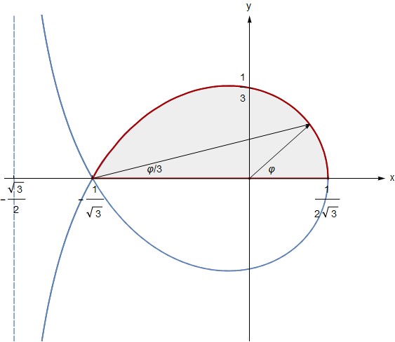
Figure 1: The trisectrix of Maclaurin intersecting x-axis at two points, $(\frac{1}{2\sqrt{3}},0)$ and $(-\frac{1}{\sqrt{3}},0)$. On $(x,y)$ plane the equation of this curve in polar coordinates $x=r\cos\varphi,\,y=r\sin\varphi\,,$ reads: $r(\varphi,\frac{1}{\sqrt{3}})=\frac{1}{2\sqrt{3}\cos({\varphi}/{3})}$ . The orbit space of a qutrit $\mathcal{O}[\mathfrak{P}_{3}]$ is given by the domain in grey.

$$\mathcal{O}[\mathfrak{P}_{3}]\,:\ \biggl{\{}\,r\geq 0\,,\varphi\in[0,\pi]\,\ \biggl{|}\,\ \cos\left(\frac{\varphi}{3}\right)\leq\frac{1}{2\sqrt{3}r}\,\biggl{\}}\,.$$ (45)

According to the analysis given in [11], the algebraic equations (3) for the eigenvalues of SW kernel of a qutrit have one-parametric solution which can be written as

$$\pi_{1}=\frac{1}{3}+\frac{2}{\sqrt{3}}\mu_{3}+\frac{2}{3}\,\mu_{8},\quad\pi_{2}=\frac{1}{3}-\frac{2}{\sqrt{3}}\mu_{3}+\frac{2}{3}\,\mu_{8},\quad\pi_{3}=\frac{1}{3}-\frac{4}{3}\,\mu_{8}\,.$$ (46)

Here the parameters $\mu_{3}$ and $\mu_{8}$ are Cartesian coordinates of a segment of a unit circle with the apex angle $\zeta$:

$$\mu_{3}=\sin\zeta\,,\qquad\mu_{8}=\cos\zeta\,,\qquad 0\leq\zeta\leq\frac{\pi}{3}\,.$$ (47)

It is worth to note that the apex angle $\zeta$ determines the value of a 3-rd order polynomial SU(3)-invariant of SW kernel $\Delta(\Omega_{3})|\nu)$:

$$\cos(3\zeta)=-\frac{27}{16}\det\left(\Delta(\Omega_{3}|\nu)\right)-\frac{11}{16}\,$$

with the moduli parameter $\nu$:

$$\nu=\frac{1}{3}-\frac{4}{3}\cos(\zeta)\,,\quad\zeta\in[0,\ {\pi}/{3}]\,.$$ (48)

Having these ingredients for a density matrix (42) and SW kernel (46), the straightforward evaluation of (36) for $N=3$ gives

$$W_{3}^{(-)} = \frac{1}{3}-\frac{4r}{\sqrt{3}}\cos\left(\zeta+\frac{\varphi}{3}-\frac{\pi}{3}\right)\,,$$ (49)

$$W_{3}^{(+)} = \frac{1}{3}+\frac{4r}{\sqrt{3}}\cos\left(\zeta-\frac{\varphi}{3}\right)\,.$$ (50)

From the expression (49) it follows that a subspace of the orbit space $\mathcal{O}[\mathfrak{P}^{(+)}_{3}]$  where WF is positive reads:

$$\mathcal{O}[\mathfrak{P}^{(+)}_{3}]\,:\biggl{\{}\,r\geq 0\,,\varphi\in[0,\pi]\,\ \biggl{|}\,\ \cos\left(\frac{\varphi}{3}+\zeta-\frac{\pi}{3}\right)\leq\frac{1}{4\sqrt{3}r}\,\biggl{\}}\,.$$ (51)

Comparing (51) with the qutrit orbit space (45) we conclude that $\mathcal{O}[\mathfrak{P}^{(+)}_{3}]$  lies inside the qutrit orbit space $\mathcal{O}[\mathfrak{P}_{3}]$ as it is shown in Fig. 2.

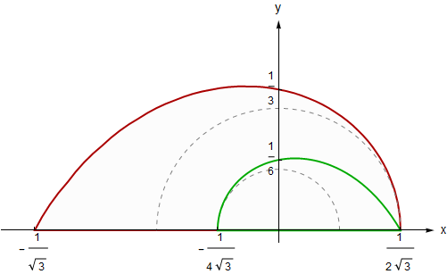
(a) $\zeta=0$

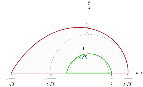
(b) $\zeta=\frac{\pi}{6}$

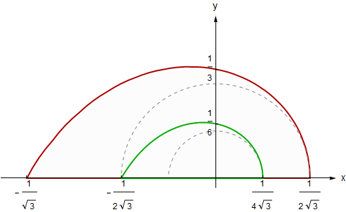
(c) $\zeta=\frac{\pi}{3}$

Figure 2: The state space of a qutrit divided into bands. The Wigner function is always positive (necessarily has some negative values) inside (outside) the region enclosed by the dashed inner (outer) semicircle regardless of the choice of the kernel. Inside the region enclosed by the kernel-dependent inner solid curve the Wigner function is always positive for the specific choice of the kernel.

Here it is in order to make few comments on a shape of $\mathcal{O}[\mathfrak{P}^{(+)}_{3}]$ :

• For $0\leq r\leq\frac{1}{4\sqrt{3}}$ the lower bound $W_{3}^{(-)}$ is positive for all $\zeta$ and $\varphi$;

• For $\frac{1}{2\sqrt{3}}\leq r\leq\frac{1}{\sqrt{3}}$ the lower bound $W_{3}^{(-)}$ is always negative;

• For intermediate values $\frac{1}{4\sqrt{3}}\leq r\leq\frac{1}{2\sqrt{3}}$ the lower bound $W_{3}^{(-)}$ becomes negative only for certain values of $\zeta$ and $\varphi$.

$\bullet$ $\mathcal{Q}$-indicator of a single qutrit  $\bullet$  The global indicator of nonclassicality of a qutrit is given by the ratio of volumes

$$\mathcal{Q}_{3}=\frac{\mbox{Vol}\left(\mathcal{O}[\mathfrak{P}^{(+)}_{3}]\right)}{\mbox{Vol}\left(\mathcal{O}[\mathfrak{P}_{3}]\right)}\,.$$ (52)

To evaluate these volume integrals we need to specify a measure on the orbit space $\mathcal{O}[\mathfrak{P}_{3}]$. Similarly to a qubit case, we assume that a qutrit state space $\mathfrak{P}_{3}$ is endowed with the Hilbert-Schmidt metric:

$$\mathrm{g}=4\,\mathrm{tr}\left(\mathrm{d}\varrho\otimes\mathrm{d}\varrho\right)\,.$$ (53)

In terms of the Bloch coordinates $\boldsymbol{\xi}=(\xi_{1},\xi_{2},\dots,\xi_{8})$ of a qutrit,

$$\varrho=\frac{1}{3}\left(\mathbb{I}+\sqrt{3}\,(\boldsymbol{\lambda},\boldsymbol{\xi})\right)\,,$$ (54)

the metric (53) gives the standard Euclidean volume form on $\mathfrak{P}_{3}$:

$$\omega=\left(\frac{8}{3}\right)^{4}\,\mathrm{d}\xi_{1}\wedge\mathrm{d}\xi_{2}\wedge\cdots\wedge\mathrm{d}\xi_{8}\,.$$ (55)

Now in order to compute the corresponding induced form on the orbit space $\mathcal{O}[\mathfrak{P}_{3}]$ , we rewrite (55) in terms of the SVD of the density matrix

$$\varrho=UDU^{{\dagger}}\,.$$ (56)

Since the measure of a singular and degenerate matrices is zero, we consider a generic spectrum $D=\mbox{diag}||r_{1},r_{2},r_{3}||$  with descending order of eigenvalues $1>r_{1}>r_{2}>r_{3}>0\,.$ This means that the arbitrariness of $U$ is given by the torus $T$ of $SU(3)$ and the volume form (55) is useful to write down in an adaptive SVD coordinates,

$$\omega=(r_{1}-r_{2})^{2}(r_{1}-r_{3})^{2}(r_{2}-r_{3})^{2}\,\mathrm{d}r_{1}\wedge\mathrm{d}r_{2}\wedge\mathrm{d}r_{3}\wedge\omega_{{}_{\mathrm{SU(3)/T}}}\,.$$ (57)

For illustrative reasons it is convenient to pass from 2-simplex Catrtesian coordinates $r_{1},r_{2},r_{3}$ to the polar variables $r$ and $\varphi\,,$ introduced in (44). As a result, the volume form (57) on the orbits space $\mathcal{O}[\mathfrak{P}_{3}]$ reduces to the following expression:

$$\omega_{\mathcal{O}[\mathfrak{P}_{3}]}=r^{7}\sin^{2}{\varphi}\,\mathrm{d}r\wedge\mathrm{d}\varphi\,.$$ (58)

Computing the volume integrals in (52) with respect to the measure (58) over the orbit space of a qutrit (45) and its subspace were WF is positive, we find an explicit dependence of the global indicator of classicality on the SW kernel moduli parameter $\zeta\,$:

$$\mathcal{Q}_{3}(\zeta)=\displaystyle{\frac{\int_{0}^{\pi}d\varphi\int_{0}^{\frac{1}{4\sqrt{3}\cos{\left(\frac{\varphi}{3}+\zeta-\frac{\pi}{3}\right)}}}r^{7}\sin^{2}(\varphi)dr}{\int_{0}^{\pi}d\varphi\int_{0}^{\frac{1}{2\sqrt{3}\cos{\frac{\varphi}{3}}}}r^{7}\sin^{2}(\varphi)dr}}=\frac{1}{128}\,\frac{1+20\cos^{2}{\left(\zeta-{\pi}/{6}\right)}}{\left(-1+4\cos^{2}{\left(\zeta-{\pi}/{6}\right)}\right)^{5}}\,.$$ (59)

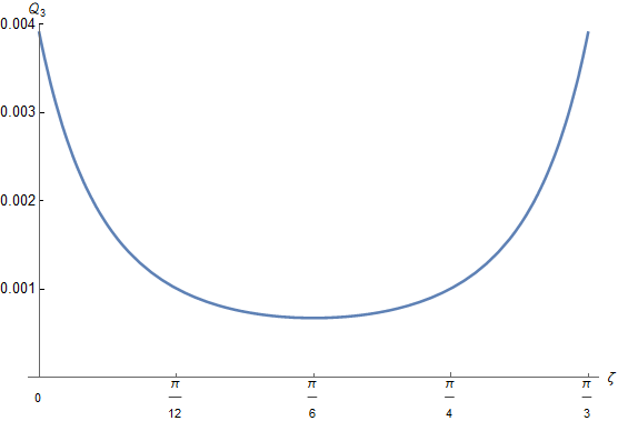
Figure 3: $\mathcal{Q}\--$indicator as a function of SW kernel moduli parameter $\zeta\,$ for the Hilbert-Schmidt qutrit.

The straightforward calculations show that the indicator $\mathcal{Q}_{3}(\zeta)$ attains the absolute minimum at a qutrit modili parameter $\zeta={\pi}/{6}\,,$

$$\min_{\zeta\in[0,\frac{\pi}{3}]}\,\mathcal{Q}_{3}(\zeta)=\mathcal{Q}_{3}\left(\frac{\pi}{6}\right)=\frac{7}{2^{7}\,3^{4}}\approx 0.000675\,,$$

corresponding to SW kernel with the spectrum:

$$\mbox{spec}\left(\Delta_{3}\right)=\biggl{|}\biggl{|}\,\frac{1+2\sqrt{3}}{3}\,,\frac{1}{3}\,,\frac{1-2\sqrt{3}}{3}\,\biggl{|}\biggl{|}\,.$$ (60)

In Fig.3 the dependence of $\mathcal{Q}_{3}$ on the moduli parameter $\zeta$ is shown.

5 Summary

In the present article we introduce the global indicator of classicality of quantum $N\--$dimensional system. This indicator directly measures the portion of its unitary orbit space which is associated to states admitting conventional statistical interpretation in terms of a true probability distributions. During the study an interesting relation between the properties of the Wigner quasiprobability distributions and structure of the Birkhoff polytopes has been found out. It seems that this relation deserves attention, and in our future publication we will come back to the problem of a classical-quantum correspondence from this point of view.

Appendix

In this Appendix we discuss the global extrema problem of a function over the unitary orbits of a Hermitian matrix.

Problem Let $A$ be a positive definite Hermitian matrix and $B$ be a Hermitian matrix. Consider the adjoint unitary orbits, $\mathcal{O}_{B}=gBg^{\dagger}\,$, with $g\in SU(N)$. Find the global extrema of the function

$$\Phi(g)=\mathrm{tr}(AgBg^{\dagger})\,.$$ (61)

To find the extrema of (61), one can apply a standard method of calculus used for a problem of determination critical points of functions. To be accurate, consider matrices $A$ and $B$ whose spectrum is of the following form:

$$\boldsymbol{\mu}^{\downarrow}(A) = \{\mu_{1}(A)\overbrace{(1,\dots,1)}^{k_{1}(A)}\,;\,\mu_{2}(A)\overbrace{(1,\dots,1)}^{k_{2}(A)}\,;\,\dots\,;\,\mu_{s}(A)\overbrace{(1,\dots,1)}^{k_{s}(A)}\}\,,$$ (62)

$$\boldsymbol{\mu}^{\downarrow}(B) = \{\mu_{1}(B)\overbrace{(1,\dots,1)}^{k_{1}(B)}\,;\,\mu_{2}(B)\overbrace{(1,\dots,1)}^{k_{2}(B)}\,;\,\dots\,;\,\mu_{s}(B)\overbrace{(1,\dots,1)}^{k_{s}(B)}\}\,.$$ (63)

The elements of spectra of both matrices are arranged in the decreasing order:

$$\mu_{1}(A)>\mu_{2}(A)>\dots>\mu_{s}(A)\qquad\mbox{and}\qquad\mu_{1}(B)>\mu_{2}(B)>\dots>\mu_{s}(B)\,.$$ (64)

The degrees of degeneracy $(k(A),k(B))$ of matrices $A$ and $B$ are constrained by the relations, $\sum_{i=1}^{s}k_{i}(A)=r_{A}$ and $\sum_{i=1}^{s}k_{i}(B)=r_{B}\,.$ The SVD decompositions for matrices

$$A=VD_{A}V^{\dagger}\,,\qquad B=WD_{B}W^{\dagger}\,$$ (65)

are not unique and a family of unitary matrices $V$ and $W$ in (65) can be built as follows. Let us denote by $V^{\downarrow}$ the unitary matrix constructed of the right eigenvectors of matrix $A$, disposed in the correspondence with the decreasing order of its eigenvalues. Then the most general family of unitary matrices diagonalizing $A$ reads

$$V=V^{\downarrow}\begin{pmatrix}V_{1}&\cdots&0\\ \vdots&\ddots&\vdots\\ 0&\cdots&V_{s}\end{pmatrix}P\,,$$ (66)

where $V_{1},\dots,V_{s}$ are arbitrary unitary matrices of order $k_{1},\dots,k_{s}$ respectively and $P$ is the transposition matrix

$$P=||\boldsymbol{e}_{i_{1}}\,,\boldsymbol{e}_{i_{2}}\,,\dots,\boldsymbol{e}_{i_{N}}||,$$

with $N\--$dimensional vectors $\boldsymbol{e}_{j}$ having everywhere zeros except 1 in the $j\--$place. The right multiplication, $AP$ , transposes the columns $j\to i_{j}\,,j=1,\dots N\,.$ Below the same construction for the unitary matrix $W$ will be used as well.

Straightforward computations show that the necessary condition of extrema for $\Phi(g)$ can be written as

$$\mathrm{d}\Phi(g)=\mbox{tr}\left([O_{B},A]w_{g}\right)=0\,,$$ (67)

where

$$w_{g}=\mathrm{d}gg^{\dagger}=\frac{\imath}{2}\,\sum_{a,i=1}^{N^{2}-1}(w_{g})^{a}_{i}\lambda_{a}\mathrm{d}\vartheta^{i}\,$$ (68)

is the Maurer-Cartan 1-form on $SU(N)\,$ group. The equation (67) tells us that extrema of $\Phi(g)$ are realized for all points of the orbits $\mathcal{O}_{B}=g_{c}Bg_{c}^{\dagger}\,,$ commuting with $A$ :

$$\ [A,\mathcal{O}_{B}]=0\,.$$ (69)

This equation has a solution $g_{c}=VW^{\dagger}$ with the unitary matrices $V$ and $W$ diagonalizing $A$ and $B$ respectively. According to (66), the matrices $V$ and $W$ constitute a family of diagonalising unitary matrices. One can see that a set of corresponding critical points $g=g_{c}$ of $\Phi(g)\,$ is discrete. As a result of (66), for given $\mbox{spec}(A)$ and $\mbox{spec}(B)$ the extrema are determined by permutations $P$

$$\Phi(g)\biggl{|}_{g=g_{c}}=\mbox{tr}(D_{A}D_{B})=\mbox{tr}\left(\boldsymbol{\mu}^{\downarrow}(A)P^{T}\boldsymbol{\mu}^{\downarrow}(B)P\right)\,.$$

Among these exrtema, the minimum and maximum are identified using the well-known result of majorisation of two vectors $x,y\in\mathbb{R}^{N}$ (cf. [15, p. 49]):

$$\langle x^{\downarrow},y^{\uparrow}\rangle\leq\langle x,y\rangle\leq\langle x^{\downarrow},y^{\downarrow}\rangle\,.$$ (70)

Hence, finally, global extrema of $\Phi(g)$ read,

$$\min_{g\in g_{c}}\Phi(g) = \mbox{tr}\left(\boldsymbol{\mu}^{\downarrow}(A)\,\boldsymbol{\mu}^{\uparrow}(B)\right)\,,$$ (71)

$$\max_{g\in g_{c}}\Phi(g) = \mbox{tr}\left(\boldsymbol{\mu}^{\downarrow}(A)\,\boldsymbol{\mu}^{\downarrow}(B)\right)\,.$$ (72)

References

• [1] H.C.F. Lemos, A.C.L. Almeida, B. Amaral, A.C. Oliveira, Roughness as classicality indicator of a quantum state, Phys. Lett. A 382, 823-836, 2018.
• [2] Anatole Kenfack and Karol Zyczkowski, Negativity of the Wigner function as an indicator of non-classicality, J. Opt. B: Quantum Semiclass. Opt. 6, 396-404, 2004.
• [3] L. Mandel, Sub-Poissonian photon statistics in resonance fluorescence, Opt. Lett. 4, 205-207, 1979.
• [4] V. Veitch, Ch. Ferrie, D. Gross and J. Emerson, Negative quasi-probability as a resource for quantum computation, New J. Phys., 14, 2012.
• [5] F. Albarelli, M.G. Genoni, Matteo G.A. Paris and A.Ferraro, Resource theory of quantum non-Gaussianity and Wigner negativity, Phys. Rev. A 98, 052350, 2018.
• [6] E.P. Wigner, Quantum-mechanical distribution functions revisited, Part I: Physical Chemistry. Part II: Solid State Physics, 251-262, 1997.
• [7] Ch. Ferrie, R. Morris and J. Emerson, Necessity of negativity in quantum theory, Phys. Rev. A 82, 044103, 2010.
• [8] R.F. O’Connell, E.P. Wigner, Quantum-Mechanical Distribution Functions: Conditions for Uniqueness, Phys. Lett. A 83, 145-148, 1981.
• [9] R.F. O’Connell and E.P. Wigner, Manifestations of Bose and Fermi statistics on the quantum distribution function for systems of spin-0 and spin-1/2 particles, Phys. Rev. A 30, 2613, 1984.
• [10] Vahagn Abgaryan and Arsen Khvedelidze, On families of Wigner functions for N-level quantum systems, https://arxiv.org/pdf/1708.05981.pdf (2018).
• [11] V. Abgaryan, A. Khvedelidze and A. Torosyan, On moduli space of the Wigner quasiprobability distributions for N-dimensional quantum systems, Zapiski Nauch. Sem. POMI 468, 177-201, 2018.
• [12] Karol Zyczkowski, Hans-Juergen Sommers, Hilbert–Schmidt volume of the set of mixed quantum states, J. Phys. A: Math. Gen. 36, 10115, 2003.
• [13] I. Daubechies, Continuity statements and counterintuitive examples in connection with Weyl quantization, J. Math. Phys., 24, 1453, 1982.
• [14] I. Bengtsson, A. Ericsson, M. Kus, W. Tadej and K.Zyczkowski, Birkhoff’s Polytope and Unistochastic Matrices, N = 3 and N = 4, Commun. Math. Phys. 259, 307-324, 2005.
• [15] Rajendra Bhatia, Majorisation and Doubly Stochastic Matrices. In: Matrix Analysis, Graduate Texts in Mathematics 169, Springer, 1997.