Large impact parameter behaviour in the CGC/saturation approach: a new non-linear equation.

Abstract

In this paper we propose a solution to the long standing problem in the CGC/saturation approach: the power-like fall off of the scattering amplitudes at large $b$. We propose a new non-linear equation, which takes into account random walks both in transverse momenta of the produced gluons and in their impact parameters. We demonstrate, that this equation is in accord with previous attempts to include the diffusion in impact parameters in the BFKL evolution equation. We show in the paper, that the solution to a new equation results in the exponential decrease of the scattering amplitude at large impact parameter, and in the restoration of the Froissart theorem.

I Introduction

It is well known that perturbative QCD has a fundamental problem: the scattering amplitude decreases at large impact parameters ($b$) as a power of $b$. In particular, the CGC/saturation approachKOLEB , which is based on perturbative QCD, is confronted by this problem. At large $b$ the scattering amplitude is small and, therefore, only the linear BFKL equationBFKL is determined by the scattering amplitude in perturbative QCD. It is known that the eigenfunction of this equation (the scattering amplitude of two dipoles with sizes $r$ and $R$) has the following formLIP

$$\phi_{\gamma}\left(\boldsymbol{r},\boldsymbol{R},\boldsymbol{b}\right)\,\,\,=\,\,\,\left(\frac{r^{2}\,R^{2}}{\left(\boldsymbol{b}+\frac{1}{2}(\boldsymbol{r}-\boldsymbol{R})\right)^{2}\,\left(\boldsymbol{b}-\frac{1}{2}(\boldsymbol{r}-\boldsymbol{R})\right)^{2}}\right)^{\gamma}\,\,\xrightarrow{b\,\gg\,r,R}\,\,\left(\frac{r^{2}\,R^{2}}{b^{4}}\right)^{\gamma}\,\,\equiv\,\,e^{\gamma\,\xi}~{}~{}\mbox{with}~{}~{}\xi\,=\,\ln\left(\frac{r^{2}\,R^{2}}{b^{4}}\right)$$ (1)

One can see that at large impact parameter $b$ the amplitude has a power-like decrease, which leads to the violation of the Froissart theoremFROI . The violation of the Froissart theorem stems from the growth of the radius of interaction as a power of the energy. Since in Ref.LIP it was proven that the eigenfunction of any kernel with conformal symmetry has the form of Eq. (1), we can only change the large $b$ behaviour by introducing a new dimensional scale in the kernel of the equation. The problem has been known from the beginning of the saturation approachLERYB1 ; LERYB2 and several ideas have been proposed, of how to introduce a new dimensional scale in the kernel of the BFKL equation (See Refs.LERYB1 ; LERYB2 ; LETAN ; QCD2 ; KHLE ; KKL ). However, for the high energy community at large, the problem was appreciated only after the papers of Refs.KW ; FIIM were published, where it was demonstrated, that the violation of the Froissart theorem cannot be avoided in the framework of the CGC approach.

First, we wish to illustrate why the Froissart theorem is violated for the BFKL equation. The general solution to the BFKL for the dipole scattering amplitude equation, has the following form:

$$N\left(r,Y;b\right)\,\,\,=\,\,\,\int^{\epsilon+i\infty}_{\epsilon-i\infty}\frac{d\gamma}{2\,\pi\,i}e^{\omega\left(\bar{\alpha}_{S},\gamma\right)\,Y}\,\phi_{\gamma}\left(\boldsymbol{r},\boldsymbol{R},\boldsymbol{b}\right)\phi_{\rm in}\left(\gamma\right)\,\,=\,\,\int^{\epsilon+i\infty}_{\epsilon-i\infty}\frac{d\gamma}{2\,\pi\,i}e^{\omega\left(\bar{\alpha}_{S},\gamma\right)\,Y\,\,+\,\,\gamma\,\xi}\,\phi_{\rm in}\left(\gamma\right)$$ (2)

where

$$\omega\left(\bar{\alpha}_{S},\gamma\right)\,\, = \,\,\bar{\alpha}_{S}\,\chi\left(\gamma\right)\,\,\,=\,\,\,\bar{\alpha}_{S}\left(2\psi\left(1\right)\,-\,\psi\left(\gamma\right)\,-\,\psi\left(1-\gamma\right)\right)$$

$$\,\xrightarrow{\gamma\to\frac{1}{2}} \,\omega_{0}\,\,+\,\,D\,\left(\gamma-\frac{1}{2}\right)^{2}\,\,+\,\,{\cal O}\left((\gamma-\frac{1}{2})^{3}\right)\,\,=\,\,\bar{\alpha}_{S}4\ln 2\,\,+\,\,\bar{\alpha}_{S}14\zeta\left(3\right)\left(\gamma-\frac{1}{2}\right)^{2}\,\,+\,\,{\cal O}\left((\gamma-\frac{1}{2})^{3}\right)$$

$\psi(z)$ denotes the Euler psi-function $\psi\left(z\right)=d\ln\Gamma(z)/dz$.

The main contribution in Eq. (2) stems from $\gamma\to\frac{1}{2}$, where we can use the expansion shown in Eq. (I) evaluating this integral using the method of steepest descend one can see that saddle point occurs at $\gamma_{\rm SP}=\frac{1}{2}-\frac{\xi}{2DY}\,\,\ll\,\,1$ and the amplitude is equal to

$$N\left(r,Y;b\right)\,\,\,\xrightarrow{b\,\gg\,r,R}\,\,\,\,\,\phi\left(\frac{1}{2}\right)\left(\frac{r^{2}\,R^{2}}{b^{4}}\right)^{1/2}\frac{1}{2\sqrt{DY}}e^{\omega_{0}Y\,-\,\frac{\xi^{2}}{4DY}}$$ (4)

Using Eq. (4) we can attempt to determine the upper bound from the unitarity constraints

$$2\,N\left(r,Y;b\right)\,\,=\,\,|N\left(r,Y;b\right)|^{2}\,\,+\,\,G_{in}\left(r^{2},Y;b\right)$$ (5)

where $G_{in}$ describes the contribution of all inelastic processes. Recalling that $N$ is the imaginary part of the scattering amplitude and assuming that the real part of the amplitude is small, as is the case for the BFKL equation, one can see that the unitarity constraint has the solution:

$$N=1-\exp\left(-\Omega\left(r,Y;b\right)\right)\,\,<\,\,1;~{}~{}~{}~{}~{}~{}~{}~{}~{}G_{in}\,=\,1\,-\,\exp\left(-2\Omega\left(r,Y;b\right)\right)$$ (6)

where $\Omega>0$ denotes an arbitrary function.

Now we can find the bound for the total cross section following Ref.FROI .

$$\sigma_{tot}\,\,=\,\,2\int N\left(r,Y;b\right)d^{2}b\,\,<\,\,2\int^{b_{0}}d^{2}b\,\,+\,\,\int_{b_{0}}d^{2}bN\left(r,Y;b\right)$$ (7)

We need to solve the following equation to find the value of $b_{0}$,

$$N\left(r,Y;b_{0}\right)\,=\,\,\phi\left(\frac{1}{2}\right)\left(\frac{r^{2}\,R^{2}}{b^{4}}\right)^{1/2}\frac{1}{2\sqrt{DY}}e^{\omega_{0}Y\,-\,\frac{\xi^{2}}{4DY}}\,=\,f_{0}\,<1$$ (8)

At large $Y$ this solution gives $b^{2}_{0}\propto e^{\left(D+\sqrt{D(D+4\omega_{0})}\right)Y}$ and therefore,

$$N\left(r,Y;b_{0}\right)\,\,<\,\,e^{\left(D+\sqrt{D(D+4\omega_{0})}\right)Y}$$ (9)

Note, that if for the soft amplitude of the typical form $N_{\rm soft}\propto e^{\omega_{0}Y-\mu b}$ and $b_{0}\,\propto Y$. One can see, that the first integral in Eq. (7) leads to $\sigma\,\leq\,{\rm Const}\,\,y^{2}$ , which is the Froissart theorem. This amplitude violates the Froissart theorem and can be considered only at large values of $b$ where $N_{\rm soft}<1$. However, the eikonal solution of Eq. (6) with $\Omega=N_{soft}$, satisfies the unitarity constraints and leads to the amplitude, that describes the Froissart disc: the amplitude is equal to 1 for $b<(1/\mu)Y$ and it has an edge which behaves as $N_{\rm soft}$.

We hope that this simple estimate shows, that the power-like decrease of the scattering amplitude is the source of the problem. To solve the problem in the framework of the CGC/ saturation approach we need to introduce a new dimensional scale $\mu$, in addition to the saturation momentum. In Ref.FROI it is shown that this new scale is related to the mass of the lightest hadrons. Perturbative QCD cannot reproduce the observed spectrum of hadrons, and attempting to solve this problem, we are doomed to introduce something from non-perturbative QCD estimates. Since the non-perturbative approach is still in an embryonic stage, one can only guess how to introduce this scale, which depends crucially on non-perturbative estimates in lattice QCD, on phenomenology of high energy interactions and on intuition, which comes from considering different theoretical models. We hope that more or less full list of the attempts to solve this problem, and to find and introduce a new dimensional scale appear in Refs.LERYB1 ; LERYB2 ; LETAN ; QCD2 ; KHLE ; KKL ; FIIM ; GBS1 ; BLT ; GKLMN ; HAMU ; MUMU ; BEST1 ; BEST2 ; KOLE ; LETA ; LLS ; LEPION ; KAN .

At first sight the recent papersCCM ; BCCM have questioned the need of a new dimensional scale, since they demonstrate that the next-to-leading order BFKL equation generates the exponential type of the impact parameter behavior without the need of a new dimensional scale. However, it turns outCLM that the NLO corrections do not change the power-like decrease of the scattering amplitude at large impact parameter, generating the exponential-type decreases in the large but limited region of the values of the impact parameter.

In this paper we re-visit one of the possible ways of introducing a new dimensional scale: to incorporate in the BFKL equation the diffusion in impact parameters($b$). The first such attempt was undertaken in the distant 1990’s LERYB1 ; LERYB2 and during three decades we have worked in this area LETAN ; QCD2 ; KHLE ; KKL ; BLT ; LEPION ; KAN . This is the reason that in the first part of the paper we give a brief review of these efforts, while in the second part we propose our generalization of the BFKL equation, which takes into account the diffusion on $b$ in accord with QCD estimates. We will discuss the structure of the scattering amplitude at high energies, which at the moment appears to be a black disc with the radius increasing as a power of energy. This paper is partly motivated by Ref.KAN , in which many questions concerning QCD has been formulated on the black disc behaviour at high energy from the point of boost invariance and the parton model. We hope that we answer some of these questions in this paper. In particular, we will demonstrate that QCD leads to the Froissart disc at high energies, with specific behaviour of the amplitude at the edge of this disc.

II Diffusions

II.1 Regge approach and Gribov’s diffusion in impact parameters

In the framework of the Regge approach the high energy amplitude is given by the exchange of the Pomeron, and has the following formCOL ; SOFT ; GRLEC ; LEPOM :

$$s\,N\left(s,Q_{t}\right)\equiv\,\,{\rm Im}A\left(s,Q_{T}\right)\,\,=\,\,g_{1}\left(Q_{T}\right)\,g_{2}\left(Q_{T}\right)e^{\alpha_{I\!\!P}\left(Q^{2}_{T}\right)Y}$$ (10)

where $g_{1},g_{2}$ and trajectory $\alpha_{I\!\!P}\left(Q^{2}_{T}\right)\equiv\,\,1\,+\,\Delta_{{I\!\!P}}\left(Q_{T}\right)=1+\Delta_{I\!\!P}-\alpha^{\prime}_{I\!\!P}Q^{2}_{T}+{\cal O}\left(Q^{4}_{T}\right)$ are the functions that have to be taken from the phenomenology. $Y=\ln\left(s\right)$ and $Q_{T}$ is the momentum transferred by the Pomeron . Eq. (10) can be viewed as the solution to the following equation:

$$\frac{dN\left(Y,Q_{T}\right)}{dY}\,\,=\,\,\Delta_{I\!\!P}\left(Q_{T}\right)\,N\left(Y,Q_{T}\right)$$ (11)

with the initial condition

$$N\left(Y=0,Q_{T}\right)\,\,=\,\,g_{1}\left(Q_{T}\right)\,g_{2}\left(Q_{T}\right)$$ (12)

In the impact parameter representation solution of Eq. (10) takes the form:

$$N\left(Y,b\right)\,\,=\,\,\int\frac{d^{2}Q_{T}}{\left(2\pi\right)^{2}}\,e^{i\boldsymbol{b}\cdot\boldsymbol{Q}_{T}}\,N\left(Y=0,Q_{T}\right)\,\,=\,\,g_{1}g_{2}e^{\Delta_{I\!\!P},Y}n\left(Y,b\right)~{}~{}~{}~{}\mbox{with}~{}~{}~{}n\left(Y,b\right)\,\,=\,\,\frac{1}{4\pi\alpha^{\prime}_{I\!\!P}Y}e^{-\frac{b^{2}}{4\alpha^{\prime}_{{I\!\!P}}Y}}$$ (13)

In Eq. (13) we have neglected the $Q_{T}$ dependence of $g_{1}$ and $g_{2}$ which does not contribute at high energies.

In Ref.GRLEC the simple fact is noted i.e. $n\left(Y,b\right)$ is the solution of the diffusion equation:

$$\frac{dn\left(Y,b\right)}{dY}\,\,=\,\,\alpha^{\prime}_{I\!\!P}\nabla^{2}_{b}\,n\left(Y,b\right)$$ (14)

Eq. (14) together with Eq. (10) for the total cross section:

$$\sigma_{tot}=2\,g_{1}\,g_{2}\,N\left(Y,Q_{T}=0\right)\,=\,2\,\,\,g_{1}\,g_{2}\,e^{\Delta_{I\!\!P}Y}\,\,=\,\,\sigma_{0}\,\sum_{n=0}^{\infty}\frac{\Delta_{I\!\!P}Y}{n!}\,\,$$ (15)

have very simple interpretations in the parton model. In the parton modelGRLEC ; LEPOM ; FEYN it is assumed, that we can describe the interaction by a field theory, in which all integrals over transverse momenta are convergent, and they lead to the mean transverse momentum, which does not depend on energy. In such a theory, the contribution to the total cross section of the scattering amplitude for production of $n$ partons in each order of perturbation approach, can be viewed as

$$\sigma_{n}\,\,=\,\,M_{2\to 2+n}\left(\{p_{i,T}\}\right)\prod^{n}_{i=0}d^{2}p_{i,T}dy_{i}\,\,=\,\,M_{2\to 2+n}\left(\{p_{i,T}\}\right)\prod^{n}_{i=0}d^{2}p_{i,T}\,\frac{Y^{n}}{n!}$$ (16)

In Eq. (16) we assume that in the proposed theory the amplitude is not equal to zero, when rapidities of emitted partons are equal to zero, and choose the largest contribution which comes from the ordering

$$0<y_{1}<y_{2}<\dots<y_{i}<\dots<y_{n}<Y$$ (17)

One can see that in Eq. (15) $M_{2\to 2+n}\left(\{p_{i,T}\}\right)\prod^{n}_{i=0}d^{2}p_{i,T}\,=\,\Delta_{I\!\!P}^{n}$ and from this equation we can conclude that the number of emitted partons $n\,=\,\Delta_{I\!\!P}\,Y$. The Gribov idea that the emission of partons has no other correlations except the fixed transverse momentum, can be viewed as a random walk in two dimensional space. For each emission due to uncertainty principle

$$\Delta b_{i}p_{i,T}\sim 1~{}~{}~{}~{}\mbox{or}~{}~{}~{}\Delta b_{i}\sim\frac{1}{<|p_{i,T}|>}$$ (18)

Therefore, after each emission the position of the parton will be shifted by an amount $\Delta b^{2}$ from Eq. (18), which is on average the same. After $n$ emissions, we have the picture shown in Fig. 1, and the total shift in $b$ is equal to

$$R^{2}_{int}\,\,=\,\,b^{2}_{n}\,\,=\,\,\frac{1}{<|p_{i,T}^{2}|>}\,\,=\,\,\frac{1}{<|p_{i,T}^{2}|>}\Delta_{I\!\!P}Y$$ (19)

Therefore, this diffusion reproduces the shrinkage of the diffraction peak. Indeed,

$$R^{2}\,\,=\,\,\frac{\int d^{2}b\,b^{2}\,N\left(Y,b\right)}{\int d^{2}b\,N\left(Y,b\right)}\,\,=\,\,4\,\alpha^{\prime}_{I\!\!P}\,Y$$ (20)

Comparing Eq. (19) and Eq. (20) one can see that

$$\alpha^{\prime}_{I\!\!P}\,=\,\,\frac{\Delta_{I\!\!P}}{4<|p_{i,T}^{2}|>}$$ (21)

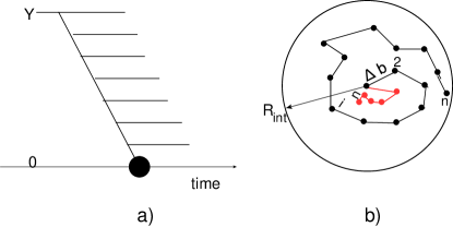
Figure 1: The structure of the parton cascade: Fig. 1-a shows the time structure of the cascade while Fig. 1-b illustrates the random walk in $b$.

Eq. (11) can be re-written in the impact parameter representation for $N\left(Y,b\right)$ of Eq. (13)

$$\frac{dN\left(Y,b\right)}{dY}\,\,=\,\,\int d^{2}b^{\prime}\,K\left(\boldsymbol{b}\,-\,\boldsymbol{b}^{\prime}\right)\,N\left(Y,b^{\prime}\right)~{}~{}~{}~{}~{}\mbox{where}\,\,K\left(b\right)\,\,=\,\int\frac{d^{2}Q_{T}}{(2\pi)^{2}}e^{i\boldsymbol{b}\,\cdot\,\boldsymbol{Q}_{T}}\Delta_{I\!\!P}\left(Q_{T}\right)$$ (22)

Let us write the equation for the radius of interaction (see Eq. (20)) . First, we see that for $\int d^{2}b\,b^{2}\,N\left(Y,b\right)=R^{2}\int d^{2}bN\left(Y,b\right)$ we have the following equation:

$$\frac{d\left(R^{2}\int d^{2}bN\left(Y,b\right)\right)}{dY}\,\,=\,\,\int d^{2}b\,d^{2}b^{\prime}\,b^{2}\,K\left(\boldsymbol{b}\,-\,\boldsymbol{b}^{\prime}\right)\,N\left(Y,b^{\prime}\right)$$

$$\,=\,\int d^{2}(\boldsymbol{b}-\boldsymbol{b}^{\prime})\,d^{2}b^{\prime}\,K\left(\boldsymbol{b}\,-\,\boldsymbol{b}^{\prime}\right)\Bigg{(}((\boldsymbol{b}-\boldsymbol{b}^{\prime})^{2}\,+2(\boldsymbol{b}-\boldsymbol{b}^{\prime})\cdot\boldsymbol{b}^{\prime}\,+\,b^{\prime 2}\Bigg{)}N\left(Y,b^{\prime}\right)\,\,$$

$$=\,\,\underbrace{\left(\int d^{2}(\boldsymbol{b}-\boldsymbol{b}^{\prime})\,\,K\left(\boldsymbol{b}\,-\,\boldsymbol{b}^{\prime}\right)((\boldsymbol{b}-\boldsymbol{b}^{\prime})^{2}\right)}_{<|\Delta b|>\Delta_{I\!\!P}\left(Q_{T}=0\right)}\int d^{2}b^{\prime}N\left(Y,b^{\prime}\right)\,\,+\,\,\underbrace{\int d^{2}(\boldsymbol{b}-\boldsymbol{b}^{\prime})\,d^{2}b^{\prime}\,K\left(\boldsymbol{b}\,-\,\boldsymbol{b}^{\prime}\right)(\boldsymbol{b}-\boldsymbol{b}^{\prime})\cdot\boldsymbol{b}^{\prime}N\left(Y,b^{\prime}\right)}_{\mbox{= 0}}$$

$$\,+\,\,\underbrace{\left(\int d^{2}(\boldsymbol{b}-\boldsymbol{b}^{\prime})\,K\left(\boldsymbol{b}\,-\,\boldsymbol{b}^{\prime}\right)\right)}_{\Delta\left(Q_{T}=0\right)}\left(\int d^{2}b^{\prime}\,b^{\prime 2}\,N\left(Y,b^{\prime}\right)\right)$$ (23)

The second term vanishes due to integration over the angle and finally we have the following equation

$$\frac{dR^{2}}{dY}\,\,=\,\,\Delta_{{I\!\!P}}<|\Delta b^{2}|>$$ (24)

with the solution $R^{2}\,=\,\Delta_{{I\!\!P}}<|\Delta b^{2}|>Y\,\,=\,\,-\nabla^{2}_{Q_{T}}\Delta_{I\!\!P}\left(Q_{T}\right)|_{Q_{T}=0}\,Y$.

We can obtain Eq. (24) using the Mueller diagramsMUDI of Fig. 2.

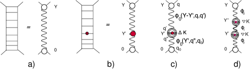
Figure 2: The Mueller diagrams for calculation of $\nabla^{2}_{Q_{T}}N\left(Y,Q_{T}\right)|_{Q_{T}=0}$. The wavy lines denote the Pomeron contribution at $Q_{T}=0$. For Fig. 2-a and Fig. 2-b it is the Pomeron in the parton model of Eq. (10), while for Fig. 2-c and Fig. 2-d it is the BFKL Pomeron in QCD(see Eq. (33). The red blobs denote $\nabla^{2}_{Q_{T}}\Delta_{I\!\!P}\left(Q_{T}\right)|_{Q_{T}=0}$ or $\nabla_{Q_{T}}\Delta_{I\!\!P}\left(Q_{T}\right)|_{Q_{T}=0}$ as it is indicated in the figures. Functions $\phi_{0}$ and $\phi_{1}$ are defined in the text.

Indeed, one can see that

$$\nabla^{2}_{Q_{T}}N\left(Y,Q_{T}\right)|_{Q_{T}=0}\,\,=\,\,-\int dY^{\prime}e^{\Delta_{I\!\!P}(Y-Y^{\prime})}\,e^{\Delta_{I\!\!P}Y^{\prime})}\nabla^{2}_{Q_{T}}\Delta_{I\!\!P}\left(Q_{T}\right)|_{Q_{T}=0}\,\,=\,\,4\alpha^{\prime}_{I\!\!P}Ye^{\Delta_{I\!\!P}Y}$$ (25)

Therefore, for $R^{2}$ we obtain $R^{2}=4\alpha^{\prime}_{I\!\!P}\,Ye^{\Delta_{I\!\!P}Y}/e^{\Delta_{I\!\!P}Y}=\,4\alpha^{\prime}_{I\!\!P}Y$ in accord with Eq. (24).

The amplitude of Eq. (13) increases with energy and violates the unitary constraints (see Eq. (5)). The eikonal unitarization of Eq. (6) leads to the following amplitude

$$N\left(Y,b\right)\,\,=\,\,1\,\,-\,\,\exp\left(-e^{\Delta_{I\!\!P}\,Y}\,\frac{1}{4\pi\alpha^{\prime}_{I\!\!P}Y}e^{-\frac{b^{2}}{4\alpha^{\prime}_{{I\!\!P}}Y}}\right)$$ (26)

One can see that this amplitude tends to unity at $b>\,\,\,\,2\,\sqrt{\Delta_{I\!\!P}\,\alpha^{\prime}_{I\!\!P}}\,Y$ leading to the total cross section $\sigma_{tot}\,\propto\,Y^{2}$ in accord with the Froissart theoremFROI .

In spite of the primitive level of calculations, especially if you compare them with typical QCD calculations in DIS, the parton model was a good guide for the Pomeron structure for years and, it is still the model where we can see all typical features of the soft Pomeron. It turns out that the time structure of the parton cascade is preserved for QCD and simple parton estimates can help develop our intuition regarding the solution of the QCD problems.

II.2 BFKL approach and diffusion in $\ln\left(p_{T}\right)$.

II.2.1 The BFKL equation.

The BFKL equation was derived in momentum representationBFKL and has the following form:

$$\frac{\partial\widetilde{N}\left(Y;q,Q_{T}\right)}{\partial Y}\,\,=\,\,\bar{\alpha}_{S}\Bigg{(}\int\frac{d^{2}q^{\prime}}{2\pi}K_{\rm em}\left(\boldsymbol{q}-\boldsymbol{q}^{\prime},\boldsymbol{Q}_{T}\right)\widetilde{N}\left(Y;q^{\prime},Q_{T}\right)\,\,-\,\,K_{\rm reg}\left(\boldsymbol{q}-\boldsymbol{q}^{\prime},\boldsymbol{Q}_{T}\right)\widetilde{N}\left(Y;q^{\prime},Q_{T}\right)\Bigg{)}$$ (27)

where $\bar{\alpha}_{S}=\left(N_{c}/\pi\right)\alpha_{S}$. Kernel $K_{\rm em}$ describes the emission of a gluon, while kernel $K_{\rm reg}$ is responsible for the reggeization of gluons in t-channel. They have the forms:

$$K_{\rm em}\left(\boldsymbol{q}-\boldsymbol{q}^{\prime},\boldsymbol{Q}_{T}\right)\,\, = \,\,\frac{1}{2}\frac{1}{\left(\boldsymbol{q}-\boldsymbol{q}^{\prime}\right)^{2}}\Bigg{\{}-\frac{Q^{2}_{T}\left(\boldsymbol{q}-\boldsymbol{q}^{\prime}\right)^{2}}{\left(\boldsymbol{Q}_{T}-\boldsymbol{q}^{\prime}\right)^{2}\,q^{\prime 2}}\,+1\,+\frac{\left(\boldsymbol{Q}_{T}-\boldsymbol{q}\right)^{2}\,q^{\prime 2}}{\left(\boldsymbol{Q}_{T}-\boldsymbol{q}^{\prime}\right)^{2}\,q^{2}}\Bigg{\}}\xrightarrow{Q_{T}=0}\frac{1}{\left(\boldsymbol{q}-\boldsymbol{q}^{\prime}\right)^{2}}$$ (28)

$$K_{\rm reg}\left(\boldsymbol{q}-\boldsymbol{q}^{\prime},\boldsymbol{Q}_{T}\right)\,\, = \frac{1}{2}\frac{1}{\left(\boldsymbol{q}-\boldsymbol{q}^{\prime}\right)^{2}}\Bigg{\{}\frac{q^{2}}{\left(\boldsymbol{q}-\boldsymbol{q}^{\prime}\right)^{2}\,+\,q^{\prime 2}}\,\,+\,\,\frac{\left(\boldsymbol{Q}_{T}\,-\,\boldsymbol{q}\right)^{2}}{\left(\boldsymbol{q}-\boldsymbol{q}^{\prime}\right)^{2}\,+\,\left(\boldsymbol{Q}_{T}-\boldsymbol{q}^{\prime}\right)^{2}}\Bigg{\}}\xrightarrow{Q_{T}=0}\frac{1}{\left(\boldsymbol{q}-\boldsymbol{q}^{\prime}\right)^{2}}\frac{q^{2}}{\left(\boldsymbol{q}-\boldsymbol{q}^{\prime}\right)^{2}\,+\,q^{\prime 2}}$$

This equation is rewritten in the coordinate representation for the scattering amplitude of a dipole with the size $r$ at impact parameter $\boldsymbol{b}$LIP ; MUCD :

$$\frac{\partial}{\partial Y}N\left(\boldsymbol{r},\boldsymbol{b},Y\right)=\bar{\alpha}_{S}\!\!\int\frac{d^{2}\boldsymbol{r}^{\prime}}{2\,\pi}\,K\left(\boldsymbol{r}^{\prime},\boldsymbol{r}-\boldsymbol{r}^{\prime};\boldsymbol{r}\right)\Bigg{(}N\left(\boldsymbol{r}^{\prime},\boldsymbol{b}-\frac{1}{2}\left(\boldsymbol{r}-\boldsymbol{r}^{\prime}\right),Y\right)+N\left(\boldsymbol{r}-\boldsymbol{r}^{\prime},\boldsymbol{b}-\frac{1}{2}\boldsymbol{r}^{\prime},Y\right)\,\,-\,\,N\left(\boldsymbol{r},\boldsymbol{b},Y\right)\Bigg{)}$$ (29)

with

$$K\left(\boldsymbol{r}^{\prime},\boldsymbol{r}-\boldsymbol{r}^{\prime};\boldsymbol{r}\right)\,\,=\,\,\frac{r^{2}}{r^{\prime 2}\,\left(\boldsymbol{r}-\boldsymbol{r}^{\prime}\right)^{2}}$$ (30)

In Eq. (29)

$$N\left(\boldsymbol{r},\boldsymbol{b},Y\right)\,\,=\,\,r^{2}\,\int\frac{d^{2}q}{2\,\pi}e^{i\boldsymbol{q}\cdot\boldsymbol{r}}\widetilde{N}\left(q,b,Y\right);~{}~{}~{}~{}~{}~{}\widetilde{N}\left(Y;q,Q_{T}\right)\,\,=\,\,\int\frac{d^{2}b}{(2\,\pi)^{2}}e^{i\boldsymbol{Q}_{T}\cdot\boldsymbol{b}}\widetilde{N}\left(q,b,Y\right);$$ (31)

II.2.2 Solutions and random walk in $\ln\left(p_{T}\right)$.

We have discussed solutions in the coordinate representation (see Eq. (1), Eq. (2) and Eq. (4)). These solutions are very useful for discussions of the non-linear corrections, since the unitarity constraints are diagonal for the dipole scattering amplitude (see Eq. (5)). However, discussing the random walk in $\ln\left(p_{T}\right)$ we need a solution in the momentum representation in which $p_{i,T}$ are the momenta of produced gluons. Note, that in Eq. (28) $\boldsymbol{q}-\boldsymbol{q}^{\prime}=\boldsymbol{p}_{T}$. For $Q_{T}$ the solution can be easily obtained, since the eigenfunction have the following formBFKL

$$\phi_{\gamma}\left(q,q_{0},Q_{T}=0\right)\,\,=\,\,\left(\frac{q^{2}}{q^{2}_{0}}\right)^{{\gamma}-1}$$ (32)

Comparing Eq. (32) with Eq. (1) one can see that $q_{0}\sim 1/R$, where $R$ denotes the size of the target. Repeating all the steps, that are given by Eq. (2) and Eq. (I), we obtain the solution in the form of Eq. (4); viz.

$$\widetilde{N}\left(q,Q_{T}=0,Y\right)\,\,\,=\,\,\,\phi\left(\frac{1}{2}\right)\left(\frac{q^{2}_{0}}{q^{2}}\right)^{1/2}\,e^{\omega_{0}\,Y}\widetilde{n}\left(q,Y\right)~{}~{}~{}\mbox{where}~{}~{}~{}\widetilde{n}\left(q,Y\right)\,\,=\,\,\frac{1}{2\sqrt{\pi\,D\,Y}}\,e^{-\,\frac{\tilde{\xi}^{2}}{4DY}}$$ (33)

with $\tilde{\xi}=\ln\left(q^{2}/q^{2}_{0}\right)$. One can recognize that for the function $n$ we have the diffusion equation in the form:

$$\frac{\partial}{\partial Y}\widetilde{n}\left(\tilde{\xi},Y\right)\,\,=\,\,D\frac{\partial^{2}}{\partial\tilde{\xi}^{2}}\widetilde{n}\left(\tilde{\xi},Y\right)$$ (34)

Therefore, the BFKL equation describes that at each emission, $\ln\left(q^{2}/q^{\prime 2}\right)$ changes its value by a constant $(\ln\left(q^{2}/q^{\prime 2}\right))^{2}=\delta$, and as a result after $n$ emissions we obtain $\ln^{2}\left(p^{2}_{T}/q^{2}_{0}\right)\,=\,\delta\,n$. Since $n=\omega_{0}\,Y$ (see the previous section) we obtain $(\ln\left(q^{2}/q^{2}_{0}\right))^{2}\,\,\delta\omega_{0}\,Y$. This estimate shows that $4D=\delta\omega_{0}$. From this estimate we see that after $n$ emissions the typical transverse momenta increase as $<|p^{2}_{T}|>\,\,=q^{2}_{0}\exp\left(\delta\,n\right)$, making the shift in $b$  $<|\Delta b^{2}|>_{n}\propto 1/<|p^{2}_{T}|>\sim(1/q^{2}_{0})\exp\left(-\delta n\right)$. Therefore, only a small number of steps at the beginning could participate in the increase of $b$ (see red lines in Fig. 1-b ).

II.2.3 The Green function of the BFKL Pomeron.

The solution of Eq. (33) can be re-written in the following form:

$$\widetilde{N}\left(q,Q_{T}=0,Y\right)\,\,\,=\,\,\,\int^{\epsilon+i\infty}_{\epsilon-i\infty}\frac{d\omega}{2\pi i}\,\int^{\epsilon+i\infty}_{\epsilon-i\infty}\frac{d\gamma}{2\pi i}\frac{1}{\omega-\omega\left(\gamma\right)}e^{\omega Y+\left(\gamma-1\right)\tilde{\xi}}\phi_{int}\left(\gamma\right)$$ (35)

We introduce the Green function of the BFKL Pomeron as follows:

$$G^{\rm BFKL}\left(\omega,\tilde{\xi}\right)\,\,\,=\,\,\,\,\int^{\epsilon+i\infty}_{\epsilon-i\infty}\frac{d\gamma}{2\pi i}\frac{1}{\omega-\omega\left(\gamma\right)}e^{\omega Y+\left(\gamma-1\right)\tilde{\xi}}$$ (36)

The Green function in $Y$ representation can be calculated as

$$G^{\rm BFKL}\left(Y,\tilde{\xi}\right)\,\,\, = \,\,\,\frac{1}{q^{2}_{0}}\int^{\epsilon+i\infty}_{\epsilon-i\infty}\frac{d\omega}{2\pi i}G^{\rm BFKL}\left(\omega,\tilde{\xi};Q_{T}=0\right)\,\,=\,\,\,\frac{1}{q^{2}_{0}}\int^{\epsilon+i\infty}_{\epsilon-i\infty}\frac{d\omega}{2\pi i}\,\int^{\epsilon+i\infty}_{\epsilon-i\infty}\frac{d\gamma}{2\pi i}\frac{1}{\omega-\omega\left(\gamma\right)}e^{\omega Y+\left(\gamma-1\right)\tilde{\xi}}$$ (37)

$$\xrightarrow{\gamma=\frac{1}{2}+i\nu,\nu\ll 1} \frac{1}{q\,q_{0}}e^{\omega_{0}\,Y}\int^{\epsilon+i\infty}_{\epsilon-i\infty}\frac{d\omega}{2\,\pi\,i}\,\frac{1}{2\,D\,\kappa_{0}}e^{-D\,\kappa^{2}_{0}\,Y\,+\,\kappa_{0}\,\,\tilde{\xi}}~{}~{}~{}\mbox{where}~{}~{}~{}\kappa_{0}\,\,=\,\,\sqrt{\frac{\left(\omega\,\,-\,\,\omega_{0}\right)}{D}}$$

Integrating over $\kappa_{0}$ we obtain the solution of Eq. (33).

One can see that $G^{\rm BFKL}\left(Y=0,\tilde{\xi};Q_{T}=0\right)=\delta\left(\tilde{\xi}\right)$ and therefore, the scattering amplitude can be found $\widetilde{N}\left(Y;q,Q_{T}=0\right)\,\,=\,\,\int d\tilde{\xi}_{0}\,G^{\rm BFKL}\left(\tilde{\xi}-\tilde{\xi}_{0}\right)\,\Phi_{in}\left(\tilde{\xi}_{0}\right)$, where $\Phi$ is the initial condition for the scattering amplitude. It should also be mentioned that factors $1/(q\,q_{0})$ are absorbed in integration of $\tilde{\xi}$ in the diagrams for Pomeron interactions.

II.2.4 The BFKL approach: random walk in $b$.

As one can see from Eq. (33) we have introduced a new dimensional scale: $q_{0}$. It was introduced as the non-perturbative size of the target $q_{0}\sim 1/R$, but its actual meaning is the separation scale: in perturbative QCD we can calculate only for $p_{T}>q_{0}$, while smaller transverse momenta have to be treated in non-perturbative approaches. From the solution of Eq. (33) one can see that the probabilty to have $p_{T}=q_{0}$ is small $\propto\,\frac{1}{2\sqrt{D\,Y}}$ but not negligible. The gluons with transverse momenta of the order of $q_{0}$ could participate in the random walk in $b$, leading to LERYB1 ; LERYB2

$$<|b^{2}|>_{n}\,=\,\frac{1}{q^{2}_{0}}P^{n}_{q_{0}}\,n\,\,\propto\,\,\,\frac{1}{q^{2}_{0}}\,\frac{1}{\sqrt{n}}\,n\propto\frac{1}{q^{2}_{0}}\sqrt{Y}$$ (38)

where $P^{n}_{q_{0}}$ denotes the probability to have the minimum momentum after $n$ emissions. In Refs.LERYB1 ; LERYB2 the numerical coefficient in Eq. (38) is evaluated. Since the average $<|b^{2}|>_{n}$ diverges at small $q$, in some sense the value of the coefficient is not important. However, we feel it is instructive to understand two qualitative features: the infrared divergency and the energy dependence.

First, we calculate the main ingredients of the calculation that we have discussed in section II-A :

$$\nabla_{Q_{T}}K_{\rm em}\left(\boldsymbol{q}-\boldsymbol{q}^{\prime},\boldsymbol{Q}_{T}\right)\Big{|}_{Q_{T}=0}\, = -\frac{1}{\left(\boldsymbol{q}-\boldsymbol{q}^{\prime}\right)^{2}}\Bigg{(}\frac{\boldsymbol{q}}{q^{2}}\,-\,\frac{\boldsymbol{q^{\prime}}}{q^{\prime 2}}\Bigg{)};$$

$$\nabla_{Q_{T}}K_{\rm reg}\left(\boldsymbol{q}-\boldsymbol{q}^{\prime},\boldsymbol{Q}_{T}\right)\Big{|}_{Q_{t}=0}\, = -\frac{1}{\left(\boldsymbol{q}-\boldsymbol{q}^{\prime}\right)^{2}}\Bigg{(}\frac{\boldsymbol{q}}{q^{\prime 2}}\,-\,\frac{\boldsymbol{q^{\prime}}\,q^{2}}{q^{\prime 4}}\Bigg{)};$$

$$-\nabla^{2}_{Q_{T}}K_{\rm em}\left(\boldsymbol{q}-\boldsymbol{q}^{\prime},\boldsymbol{Q}_{T}\right)\Big{|}_{Q_{T}=0}\, = \,-\Delta_{Q_{T}}K_{\rm em}\left(\boldsymbol{q}-\boldsymbol{q}^{\prime},\boldsymbol{Q}_{T}\right)\Big{|}_{Q_{T}=0}\,\,=\,\,\frac{2}{q^{2}\,q^{\prime 2}};$$

$$\Delta_{Q_{T}}K_{\rm reg}\left(\boldsymbol{q}-\boldsymbol{q}^{\prime},\boldsymbol{Q}_{T}\right)\Big{|}_{Q_{T}=0}\,\, = \,\,0$$ (39)

As we have discussed in section II-A (see Eq. (II.1)), we can write the equation for $-\nabla^{2}_{Q_{T}}\widetilde{N}\left(Y;q,Q_{T}\right)|_{Q_{T}=0}\,\,=\,\,\int\frac{d^{2}b}{(2\,\pi)^{2}}\,b^{2}\,\widetilde{N}\left(q,b,Y\right)$ applying $-\nabla^{2}_{Q_{T}}$ to the both parts of Eq. (27). In doing so, we obtain:

$$\frac{\partial}{\partial Y}\left(-\nabla^{2}_{Q_{T}}\widetilde{N}\left(Y;q,Q_{T}\right)|_{Q_{T}=0}\right) = \int d^{2}q^{\prime}\nabla^{2}_{Q_{T}}K\left(\boldsymbol{q}-\boldsymbol{q}^{\prime},\boldsymbol{Q}_{T}\right)\Big{|}_{Q_{T}=0}\widetilde{N}\left(Y;q^{\prime},Q_{T}\right)|_{Q_{T}=0}$$ (40)

$$- 2\int d^{2}q^{\prime}\nabla_{Q_{T}}K\left(\boldsymbol{q}-\boldsymbol{q}^{\prime},\boldsymbol{Q}_{T}\right)\Big{|}_{Q_{T}=0}\cdot\left(\nabla_{Q_{T}}\widetilde{N}\left(Y;q^{\prime},Q_{T}\right)|_{Q_{T}=0}\right)$$

$$\,\,+\,\, \int d^{2}q^{\prime}K\left(\boldsymbol{q}-\boldsymbol{q}^{\prime},\boldsymbol{Q}_{T}\right)\Big{|}_{Q_{T}=0}\left(-\nabla^{2}_{Q_{T}}\widetilde{N}\left(Y;q^{\prime},Q_{T}\right)|_{Q_{T}=0}\right)$$

To obtain the complete system of equations we need to add the equation for $\nabla_{Q_{T}}\widetilde{N}\left(Y;q^{\prime},Q_{T}\right)|_{Q_{T}=0}$. It takes the form:

$$\frac{\partial}{\partial Y}\left(\nabla_{Q_{T}}\widetilde{N}\left(Y;q,Q_{T}\right)|_{Q_{T}=0}\right) = \int d^{2}q^{\prime}\nabla_{Q_{T}}K\left(\boldsymbol{q}-\boldsymbol{q}^{\prime},\boldsymbol{Q}_{T}\right)\Big{|}_{Q_{T}=0}\widetilde{N}\left(Y;q^{\prime},Q_{T}\right)|_{Q_{T}=0}$$ (41)

$$+ \int d^{2}q^{\prime}K\left(\boldsymbol{q}-\boldsymbol{q}^{\prime},\boldsymbol{Q}_{T}\right)\Big{|}_{Q_{T}=0}\left(\nabla_{Q_{T}}\widetilde{N}\left(Y;q^{\prime},Q_{T}\right)|_{Q_{T}=0}\right)$$

Eq. (41) can be re-written as

$$\left(\frac{\partial}{\partial Y}-1\right)\nabla_{Q_{T}}\widetilde{N}\left(Y;q,Q_{T}\right)|_{Q_{T}=0}\,=\,\bar{\alpha}_{S}\frac{\boldsymbol{q}}{q^{2}}\Bigg{(}\int_{q^{2}}\frac{dq^{\prime 2}}{q^{\prime 2}}\widetilde{N}\left(Y;q^{\prime},Q_{T}=0\right)\,-\,\widetilde{N}\left(Y;q,Q_{T}=0\right)\Bigg{)}$$ (42)

In the double Mellin transform of Eq. (36) the solution to Eq. (42) has the form:

$$\nabla_{Q_{T}}\widetilde{N}\left(\omega;\gamma,Q_{T}\right)|_{Q_{T}=0}\,=\,\bar{\alpha}_{S}\,\frac{\boldsymbol{q}}{q^{2}}\frac{1}{\omega-\omega\left(\gamma\right)}\Bigg{(}\frac{1}{1-\gamma}\,-\,1\Bigg{)}$$ (43)

Plugging the solution of Eq. (43) into Eq. (40), we reduce this equation to the following one:

$$\frac{\partial}{\partial Y}\left(-\nabla^{2}_{Q_{T}}\widetilde{N}\left(Y;q,Q_{T}\right)|_{Q_{T}=0}\right)\,\,-\,\,\int d^{2}q^{\prime}K\left(\boldsymbol{q}-\boldsymbol{q}^{\prime},\boldsymbol{Q}_{T}=0\right)\left(-\nabla^{2}_{Q_{T}}\widetilde{N}\left(Y;q^{\prime},Q_{T}\right)|_{Q_{T}=0}\right)=$$

$$\,\,2\,\frac{\bar{\alpha}_{S}}{q^{2}}\Bigg{\{}\int^{\infty}_{0}\frac{dq^{\prime 2}}{q^{\prime 2}}\widetilde{N}\left(Y;q^{\prime},Q_{T}=0\right)\,+\,2\,\bar{\alpha}_{S}\int^{q^{2}}_{0}\frac{dq^{\prime 2}}{q^{\prime 2}}\int^{\epsilon+i\infty}_{\epsilon-i\infty}\frac{d\gamma}{2\pi i}\frac{1}{\omega-\omega\left(\gamma\right)}\Bigg{(}\frac{1}{1-\gamma}\,-\,1\Bigg{)}e^{\omega Y+\left(\gamma-1\right)\tilde{\xi}}\Bigg{\}}$$ (44)

The main contributions to the integrals over $q^{\prime}$ stems from the region $q^{\prime}\to 0$, Taking this into account the solution in the $\omega$- representation takes the form:

$$\nabla^{2}_{Q_{T}}\widetilde{N}\left(\omega;q,Q_{T}\right)|_{Q_{T}=0}\,\,=\,\,2\,\frac{\bar{\alpha}_{S}}{q^{2}}\frac{1+\bar{\alpha}_{S}}{D^{2}\kappa_{0}^{2}}\,\,\propto\,\,\frac{1}{\omega-\omega_{0}}$$ (45)

Therefore, we see from Eq. (45) that $\nabla^{2}_{Q_{T}}\widetilde{N}\left(\omega;q,Q_{T}\right)|_{Q_{T}=0}\propto e^{\omega_{0}Y}$

We need to divide this solution by the $\widetilde{N}\left(Y;q^{\prime},Q_{T}\right)|_{Q_{T}=0}$ and finally, we obtain for $\xi^{2}\ll D\,Y$ that

$$\left\langle b^{2}\right\rangle\,\,=\,\,2\bar{\alpha}_{S}(1+\bar{\alpha}_{S})\,\sqrt{\frac{\pi}{D}}\,\frac{1}{q^{2}}\,\sqrt{Y}\,\,=\,\,\alpha^{\prime}_{\rm eff}\,\sqrt{Y}$$ (46)

As was shown in RefsLERYB1 ; LERYB2 , the second term does not have the suppression of the order of $\bar{\alpha}_{S}$, as we can see from Eq. (45). Such an enhancement comes from the replacement in Eq. (40)

$$2\int d^{2}q^{\prime}\nabla_{Q_{T}}K\left(\boldsymbol{q}-\boldsymbol{q}^{\prime},\boldsymbol{Q}_{T}\right)\Big{|}_{Q_{T}=0}\cdot\left(\nabla_{Q_{T}}\widetilde{N}\left(Y;q^{\prime},Q_{T}\right)|_{Q_{T}=0}\right)\,\to\,$$

$$2\int d^{2}q^{\prime}\nabla_{Q_{T}}K\left(\boldsymbol{q}-\boldsymbol{q}^{\prime},\boldsymbol{Q}_{T}\right)\Big{|}_{Q_{T}=0}\bigotimes\phi_{1}\left(Y-Y^{\prime},q",q^{\prime},\theta\right)\bigotimes\left(\nabla_{Q_{T}}\widetilde{N}\left(Y^{\prime};q",Q_{T}\right)|_{Q_{T}=0}\right)$$ (47)

$\bigotimes$ stands for all needed integrations. The eigenfunction $\phi_{1}$LIP depends on the angles between $\boldsymbol{q}"$ and $\boldsymbol{q}^{\prime}$ and has an intercept which is negative and $\propto\,\bar{\alpha}_{S}$. Integration over $Y^{\prime}$ leads to the factor $1/\bar{\alpha}_{S}$ which compensates the small value of $\bar{\alpha}_{S}$. This contribution actually leads to the change of the numerical coefficient, which does not have much meaning, since $\left\langle b^{2}\right\rangle$ is infrared unstable and $q\to q_{0}$ gives the main contribution. The value of the scale $q_{0}$ is not determined in our approach. Hence, we introduce a new dimensional scale $\alpha^{\prime}_{\rm eff}$ which, we hope, will heal the large $b$ behaviour of the scattering amplitude.

III Searching for a new dimensional scale in the CGC/saturation approach

In this section we would like to give a brief review of the attempts to introduce both the random walk in $\ln\left(p_{T}\right)$, and in $b$, in the effective theory describing QCD at high energies: the CGC/saturation approach. These efforts cover a long span in time, from the first GLR equationGLR (see also Refs.MUQI ; MV ; MUCD ) till recent papers. Our goal is to introduce the random walk in $b$ in the framework of the non-linear evolution equations, which guarantee the unitarity of the scattering amplitude.

III.1 Non-linear evolution equations in QCD

We start with the current form of the non-linear equationBK , which has the following form for the scattering amplitude of the dipole with size $\boldsymbol{r}$ and rapidity $Y$ at impact parameter $\boldsymbol{b}$:

$$\frac{\partial}{\partial Y}N\left(\boldsymbol{r},\boldsymbol{b},Y\right) = \bar{\alpha}_{S}\!\!\int\frac{d^{2}\boldsymbol{r}^{\prime}}{2\,\pi}\,K\left(\boldsymbol{r}^{\prime},\boldsymbol{r}-\boldsymbol{r}^{\prime};\boldsymbol{r}\right)\Bigg{\{}N\left(\boldsymbol{r}^{\prime},\boldsymbol{b}-\frac{1}{2}\left(\boldsymbol{r}-\boldsymbol{r}^{\prime}\right),Y\right)+N\left(\boldsymbol{r}-\boldsymbol{r}^{\prime},\boldsymbol{b}-\frac{1}{2}\boldsymbol{r}^{\prime},Y\right)\,\,-\,\,N\left(\boldsymbol{r},\boldsymbol{b},Y\right)$$ (48)

$$~{}~{}~{}~{}~{}~{}~{}~{}~{}~{}~{}~{}~{}~{}~{}~{}~{}~{}~{}~{}~{}~{}~{}~{}~{}~{}~{}~{}~{}~{}~{}~{}~{}-N\left(\boldsymbol{r}-\boldsymbol{r}^{\prime},\boldsymbol{b}-\frac{1}{2}\boldsymbol{r}^{\prime},Y\right)\,N\left(\boldsymbol{r}^{\prime},\boldsymbol{b}-\frac{1}{2}\left(\boldsymbol{r}-\boldsymbol{r}^{\prime}\right),Y\right)\Bigg{\}}$$

The kernel $K\left(\boldsymbol{r}^{\prime},\boldsymbol{r}-\boldsymbol{r}^{\prime};\boldsymbol{r}\right)$ is given by Eq. (30). For $\widetilde{N}\left(Y;q,Q_{T}\right)$ and $\widetilde{N}\left(q,b,Y\right)$ (see Eq. (31) ) can be re-written in the forms:

$$\frac{\partial\widetilde{N}\left(Y;q,Q_{T}\right)}{\partial Y}\,\, = \,\,\bar{\alpha}_{S}\Bigg{\{}\int\frac{d^{2}q^{\prime}}{2\pi}K_{\rm em}\left(\boldsymbol{q}-\boldsymbol{q}^{\prime},\boldsymbol{Q}_{T}\right)\widetilde{N}\left(Y;q^{\prime},Q_{T}\right)\,\,-\,\,K_{\rm reg}\left(\boldsymbol{q}-\boldsymbol{q}^{\prime},\boldsymbol{Q}_{T}\right)\widetilde{N}\left(Y;q^{\prime},Q_{T}\right)$$ (49)

$$- \,\,\int\frac{d^{2}Q^{\prime}_{T}}{4\pi^{2}}\widetilde{N}\left(Y;q^{\prime},\boldsymbol{Q}_{T}-\boldsymbol{Q}^{\prime}_{T}\right)\,\widetilde{N}\left(Y;q^{\prime},\boldsymbol{Q}^{\prime}_{T}\right)\Bigg{\}}$$

with the kernels from Eq. (28).

Finally, for $b\,\gg\,max\{r,r^{\prime}\}$ Eq. (49) can be simplified (see Ref.KOLEB ) to

$$\frac{\partial\widetilde{N}\left(Y;q,b\right)}{\partial Y} =$$

$$\bar{\alpha}_{S}\Bigg{\{}\int\frac{d^{2}q^{\prime}}{2\pi}K_{\rm em}\left(\boldsymbol{q}-\boldsymbol{q}^{\prime},Q_{T}=0\right)\widetilde{N}\left(Y;q^{\prime},b\right)\,\,-\,\,K_{\rm reg}\left(\boldsymbol{q}-\boldsymbol{q}^{\prime},Q_{T}=0\right)\widetilde{N}\left(Y;q,b\right)\,\,-\,\,\left(\widetilde{N}\left(Y;q^{\prime},b\right)\right)\Bigg{\}}$$

III.2 The GLR equation

The first non-linear equation GLR addressed the problem of large $b$ behaviour of the scattering amplitude. The non-linear evolution equations of the previous subsections can be viewed as the sum of the ‘fan’ diagrams (see Fig. 3 for the example of such diagrams). It was shown in Ref.GLR that integrations over all transfer momenta $Q^{\prime}_{T}$ carried by the BFKL Pomerons in such diagrams, (see Fig. 3 for example) turns out to be of the order of $Q"_{T}\sim 1/R_{h}$, where $R_{h}$ is the size of the hadron target. Therefore, if the dipole sizes are much smaller than $R_{h}$, as it is for deep inelastic processes, we can replace $\widetilde{N}\left(Y;q,Q_{T}\right)$ in Eq. (49) by $\widetilde{N}\left(Y;q,Q_{T}=0\right)S\left(Q_{T}\right)$ and reduce Eq. (49) to the GLR equation

$$\frac{\partial\widetilde{N}\left(Y;q,Q_{T}=0\right)}{\partial Y}\,=$$ (51)

$$\,\,\bar{\alpha}_{S}\Bigg{\{}\int\frac{d^{2}q^{\prime}}{2\pi}K_{\rm em}\left(\boldsymbol{q}-\boldsymbol{q}^{\prime},\boldsymbol{Q}_{T}=0\right)\widetilde{N}\left(Y;q^{\prime},Q_{T}\right)\,\,-\,\,K_{\rm reg}\left(\boldsymbol{q}-\boldsymbol{q}^{\prime},\boldsymbol{Q}_{T}=0\right)\widetilde{N}\left(Y;q^{\prime},Q_{T}=0\right)-\,\,\frac{1}{S_{h}}\widetilde{N}^{2}\left(Y;q^{\prime},\boldsymbol{Q}_{T}=0\right)\Bigg{\}}$$

where $\frac{1}{S_{h}}\,=\,\int\frac{d^{2}Q^{\prime}_{T}}{4\pi^{2}}S^{2}\left(Q^{\prime}_{T}\right)$ is a constant which depends on the unknown non-perturbative structure of the hadrons. $S_{h}$ is the area of the hadron which is populated by gluons.

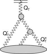
Figure 3: An example of ‘fan’ diagrams, whose sum is described by the non-linear equations. The wavy lines denote the BFKL Pomerons.

The GLR equation is written for the infrared safe observable: the gluon structure function; and it was suggested that it replace the DGLAP equation in the region of small $x$( high energies). Considering this equation we do not have a problem of the large $b$ behaviour of the amplitude. The intuition behind this equation is very transparent: in deep inelastic processes the number of gluons increases with the growth of energy, while the size of their distribution remains the same until the hadron becomes black. At ultra high energies the radius of the distribution could increase and we cannot trust the equation. From Eq. (51) we can see that the large $b$ problem is intimately related to the black disc behaviour of the scattering amplitude, and we need to develop a different equation to describe the behaviour of the edge of the disc.

III.3 The first equation incorporating both diffusions

In Ref.LERYB1 the first equation was proposed that incorporates both diffusions in $\ln\left(p_{T}\right)$ and in $b$. This equation has the form:

$$\frac{\partial\widetilde{N}\left(Y;q,b\right)}{\partial Y}\,\,=\,\,\bar{\alpha}_{S}\Bigg{\{}\int\frac{d^{2}q^{\prime}}{2\pi}\int\frac{d^{2}b^{\prime}}{2\pi}K\left(\boldsymbol{q}-\boldsymbol{q}^{\prime}\right)\left(q^{\prime 2}\,\kappa\,e^{-\kappa\,q^{\prime 2}\,(\boldsymbol{b}-\boldsymbol{b}^{\prime})^{2}}\right)\widetilde{N}\left(Y;q^{\prime},b^{\prime}\right)\,\,\,-\,\,\widetilde{N}^{2}\left(Y;q,b\right)\Bigg{\}}$$

where

$$K\left(\boldsymbol{q}-\boldsymbol{q}^{\prime}\right)\,\,=\,\,\frac{1}{\left(\boldsymbol{q}-\boldsymbol{q}^{\prime}\right)^{2}}\,\,-\,\,\frac{1}{\left(\boldsymbol{q}-\boldsymbol{q};\right)^{2}\,\,\left(\left(\boldsymbol{q}-\boldsymbol{q}^{\prime}\right)^{2}+q^{\prime 2}\right)}\delta^{(2)}\left(\boldsymbol{q}-\boldsymbol{q}^{\prime}\right)$$ (52)

At large $b$ the shadowing corrections (the non-linear term) in the equation makes a small contribution, and one can see that the new kernel leads to the same intercept of the BFKL Pomeron since it does not contribute to $\int d^{2}\widetilde{N}\left(Y;q,b\right)\equiv\widetilde{N}\left(Y;q,Q_{T}=0\right)$.

Recently, the differential form of Eq. (III.3) has been proposed in Ref.KAN , which has the form :

$$\frac{\partial\widetilde{N}\left(Y;q,b\right)}{\partial Y}\,\,=\,\,\bar{\alpha}_{S}\Bigg{\{}\int\frac{d^{2}q^{\prime}}{2\pi}\int\frac{d^{2}b^{\prime}}{2\pi}K\left(\boldsymbol{q}-\boldsymbol{q}^{\prime}\right)\widetilde{N}\left(Y;q^{\prime},b^{\prime}\right)\,\,\,-\,\,\widetilde{N}^{2}\left(Y;q,b\right)\Bigg{\}}\,+\,\frac{\kappa}{q^{2}}\,\nabla^{2}_{b}\widetilde{N}\left(Y;q,b\right)$$ (53)

Neglecting the non-linear term at large $b$ and using the function $\widetilde{N}^{2}\left(\omega;\gamma,Q_{T}\right)$ we can re-write Eq. (53) in the form:

$$\left(\omega-\omega(\gamma)\,-\,\alpha^{\prime}_{\rm eff}\,Q^{2}_{T}\right)\widetilde{N}\left(\omega;\gamma,Q_{T}\right)=0$$ (54)

with $\alpha^{\prime}_{\rm eff}=\kappa/q^{2}_{0}$. In Eq. (54) we replace $1/q^{2}$ by $1/q^{2}_{0}$ where $q_{0}$ is the smallest momentum where one can use the perturbative QCD approach.

Hence the solution takes the form:

$$\widetilde{N}\left(Y;q,b\right)\,\, = \,\,\int^{\epsilon+i\infty}_{\epsilon-i\infty}\frac{d\gamma}{2\pi\,i}\int\frac{d^{2}Q_{T}}{4\pi^{2}}e^{\omega(\gamma)\,Y\,-\,(1-\gamma)\xi\,+\,i\boldsymbol{Q}_{T}\cdot\boldsymbol{b}\,-\,\alpha^{\prime}_{\rm eff}Q^{2}_{T}}\widetilde{n}_{in}\left(\gamma\right)$$ (55)

$$= \frac{q_{0}}{q}\widetilde{n}_{in}\left(\frac{1}{2}\right)\,\left(\frac{1}{2\sqrt{\pi\,D\,Y}}e^{\omega_{0}\,Y\,-\,\frac{\xi^{2}}{4\,D\,Y}}\right)\,\left(\frac{1}{4\pi\alpha^{\prime}_{\rm eff}\,Y}e^{-\frac{b^{2}}{4\,\alpha^{\prime}_{\rm eff}\,Y}}\right)$$

Therefore, we see that indeed we have both diffusions, but the diffusion in $b$ does not have $\left\langle b^{2}\right\rangle\propto\sqrt{Y}$. Eq. (55) leads to the solution with a black disc, whose radius can be found from the equation:

$$\omega_{0}\,Y\,-\,\frac{\xi^{2}}{4\,D\,Y}-\frac{b^{2}_{0}}{4\,\alpha^{\prime}_{\rm eff}Y}\,\,=\,\,0;~{}~{}~{}~{}~{}~{}~{}b^{2}_{0}\,=\,4\,\alpha^{\prime}_{\rm eff}\,\omega_{0}\,Y^{2}\,\,-\,\,\frac{\alpha^{\prime}_{\rm eff}}{D}\,\xi^{2};$$ (56)

As we have demonstrated in section II-A Eq. (57) results in the Froissart bound;

$$\sigma\,\,\leq\,\,2\pi b^{2}_{0}=2\pi\left(4\,\alpha^{\prime}_{\rm eff}\,\omega_{0}\,Y^{2}\,\,-\,\,\frac{\alpha^{\prime}_{\rm eff}}{D}\,\xi^{2}\right)$$ (57)

The main problem with Eq. (III.3) and Eq. (53) is, that they do not reproduce the correct $\left\langle b^{2}\right\rangle\,\propto\,\sqrt{Y}$ which as we have discussed, arises in QCD.

At first sight Eq. (III.3) can lead to a different solution, but for $\widetilde{N}^{2}\left(\omega;\gamma,Q_{T}\right)$ it takes the following form:

$$\left(\omega-\omega(\gamma)\,+\,e^{-\alpha^{\prime}_{\rm eff}\,Q^{2}_{T}}-1\right)\widetilde{N}\left(\omega;\gamma,Q_{T}\right)=0$$ (58)

The solution to Eq. (58) is

$$\widetilde{N}\left(Y;q,b\right)\,\, = \,\,\int^{\epsilon+i\infty}_{\epsilon-i\infty}\frac{d\gamma}{2\pi\,i}\int\frac{d^{2}Q_{T}}{4\pi^{2}}e^{\omega(\gamma)\,Y\,-\,(1-\gamma)\xi\,+\,i\boldsymbol{Q}_{T}\cdot\boldsymbol{b}\,+\,\left(e^{-\,\alpha^{\prime}_{\rm eff}Q^{2}_{T}}-1\right)\,Y}\widetilde{n}_{in}\left(\gamma\right)$$ (59)

$$= \frac{q_{0}}{q}\widetilde{n}_{in}\left(\frac{1}{2}\right)\,\left(\frac{1}{2\sqrt{\pi\,D\,Y}}e^{\omega_{0}\,Y\,-\,\frac{\xi^{2}}{4\,D\,Y}}\right)\,\sum^{\infty}_{n=0}\left(\frac{n}{4\pi\alpha^{\prime}_{\rm eff}\,Y}\frac{Y^{n}}{n!}\,e^{-\frac{b^{2}}{4\,\alpha^{\prime}_{\rm eff}\,n}}\right)$$

$$= \frac{q_{0}}{q}\widetilde{n}_{in}\left(\frac{1}{2}\right)\,\left(\frac{1}{2\sqrt{\pi\,D\,Y}}e^{\omega_{0}\,Y\,-\,\frac{\xi^{2}}{4\,D\,Y}}\right)\,\left(\frac{1}{4\pi\alpha^{\prime}_{\rm eff}\,Y}e^{-\frac{b^{2}}{4\,\alpha^{\prime}_{\rm eff}\,Y}}\right)$$

In Eq. (59) we summed over $n$ using the method of steepest descend and used , that at $Q_{T}=0$, the $\omega(\gamma)$ spectrum is the same as in the BFKL equation.

III.4 The field theory realization of the parton model: the BFKL Pomeron in spontaneously broken QCD in 2+1 space-time dimensions

In Ref.QCD2 the BFKL Pomeron is studied in spontaneously broken 2 + 1 QCD, The coupling constant of this theory $g$ has dimension of mass, therefore, this is a super renormalizable theory which is, actually, a theoretical realization of the parton model, that has been discussed in section II-A. In this theory we do not have the ultraviolet divergencies, which results in the absence of the scaling violations, in the behaviour of the deep inelastic structure functions. On the other hand, the infrared singularities in the massless limit are stronger than in 3+1 QCD. Being such, this theory is suitable for discussing the influence of the infrared singularities on the Pomeron structure. In particular, we expect Gribov’s diffusion in the impact parameters.

The BFKL equation in this theory has the same form of Eq. (27) with replacement

$$\frac{d^{2}q^{\prime}}{4\pi^{2}}\,\,\to\,\,\frac{dq^{\prime}}{2\pi}$$ (60)

and with the change of the kernels of Eq. (28) due to inclusion of the mass of gluon $m$. It can be written as

$$\left(\omega-\alpha\left(q\right)-\alpha\left(Q_{T}-q\right)\right)\widetilde{N}\left(Y;q,Q_{T}-q\right)\,\,=$$

$$\,\,\frac{\omega}{A\left(Q_{T}\right)}\,+\,\frac{g^{2}N_{c}}{8\pi^{2}}\int\frac{d\,q^{\prime}}{\left(q^{\prime 2}+m^{2}\right)^{2}\,\left(\left(q-q^{\prime}\right)^{2}+m^{2}\right)}K\left(q,q^{\prime},Q_{T}\right)\widetilde{N}\left(Y;q^{\prime},Q_{T}-q^{\prime}\right)$$ (61)

where the gluon trajectories are

$$\alpha\left(q\right)\,=\,-\frac{g^{2}N_{c}}{8\pi^{2}}\left(q^{2}+m^{2}\right)\int\frac{d\,q^{\prime}}{\left(q^{\prime 2}+m^{2}\right)\,\left((q-q^{\prime})^{2}+m^{2}\right)}\,=\,\alpha_{S}\frac{q^{2}+m^{2}}{q^{2}+4m^{2}}$$ (62)

where $\alpha_{S}=g^{2}\,N_{c}/(4\pi m)$ ($N_{c}$ denotes the number of colours).

$$K\left(q,q-q^{\prime},Q_{T}\right)\,\,=\,\,A\left(Q_{T}\right)+\frac{2}{(q-q^{\prime})^{2}+m^{2}}\Bigg{(}\frac{q^{2}+m^{2}}{q^{\prime 2}+m^{2}}+\frac{(Q_{T}-q)^{2}+m^{2}}{Q_{T}-q^{\prime})^{2}+m^{2}}\Bigg{)}~{}~{}\mbox{with}~{}~{}A(Q_{T})=-2\left(Q^{2}_{T}+\frac{N_{c}+1}{N_{c}}\,m^{2}\right)$$ (63)

Eq. (III.4) is solved analytically in Ref.QCD2 , both in coordinate and momentum representations. It turns out that the rightmost singularity in $\omega$ is the Regge pole with the trajectory

$$\alpha_{I\!\!P}\left(Q_{T}\right)\,\,=\,\,1\,\,+\Delta^{(2)}\,\,-\,\,\alpha^{\prime(2)}_{I\!\!P}\,Q^{2}_{T}$$ (64)

with $\Delta^{(2)}=\alpha_{S}/\epsilon^{3})$ ($\epsilon^{3}$ = 3.8) and $\alpha^{\prime(2)}_{I\!\!P}=0.34\frac{\alpha_{S}}{m^{2}}$. However, at $\omega=0$ there exists a standing branch point. For $Q^{2}_{T}\to\infty$ the Regge pole approaches $\omega=0$. The trajectory of Eq. (64) means that the scattering amplitude has the following form

$$\widetilde{N}\left(Y;q,b\right)\,\,=\,\,e^{\Delta^{(2)}\,Y}\left(\sqrt{\frac{\pi}{\alpha^{\prime(2)}_{I\!\!P}\,Y}}\,e^{-\frac{b^{2}}{4\alpha^{\prime(2)}_{I\!\!P}\,Y}}\right)$$ (65)

The dependence on the sizes of the scattering dipoles or on their transverse momenta, only enters the vertices of the interactions of this Regge pole with the particles. Therefore, in this theory we obtain the typical soft Pomeron of the parton model, with the diffusion in $b$ but without random walk in $\ln\left(p_{T}\right)$.

III.5 The hierarchy of scales: the interface of soft and hard Pomerons.

In the previous section we saw, that the infrared divergency could generate the soft Pomeron: the Reggeon with the intercept larger than 1 and with the trajectory of the type of Eq. (64). However, such a soft Pomeron should exist simultaneously with the BFKL Pomeron, and we have to find the high energy asymptotic behaviour of the scattering amplitude, taking into account the interface of these two Pomerons. The second problem is to find a new dimensional scale, which in the spontaneously broken 2 + 1 QCD is the coupling constant $g$, which has the dimension of mass.

In Ref.KHLE it is shown that such a scale exists in the QCD vacuum as a consequence of scale anomaly, and it is related to the density of vacuum gluon fields due to semi–classical fluctuations: numerically, $M_{0}^{2}\simeq 4\div 6$ GeV² . Fig. 4-b and Fig. 4-c illustrate how this new scale enters the structure of the soft Pomeron. Indeed, among the higher order, $O(\alpha^{2}_{S})$ ($\alpha_{S}=g^{2}/4\pi$) corrections, to the BFKL kernel (see Fig. 4-b). We isolate a particular class of diagrams, which include the propagation of two gluons in the scalar color singlet channel $J^{PC}=0^{++}$. The vertex of their production, generated the four-gluon coupling in the QCD Lagrangian, is $\sim\alpha_{s}F^{\mu\nu\ a}F_{\mu\nu}^{a}$. We observe, that this vertex is proportional to the trace of the QCD energy–momentum tensor ( $\theta^{\mu}_{\mu}$) in the chiral limit of massless quarks:

$$\theta_{\mu}^{\mu}=\frac{\beta(g)}{2g}F^{a\alpha\beta}F_{\alpha\beta}^{a}\simeq-\frac{bg^{2}}{32\pi^{2}}F^{a\alpha\beta}F_{\alpha\beta}^{a};$$ (66)

The contribution of Fig. 4-b, therefore, appears proportional to the correlator of the QCD energy - momentum tensor, for which we have

$$\Pi(q^{2})=i\int d^{4}x\ e^{iqx}\ \left\langle 0\right|\mbox{T}\left\{\theta_{\mu}^{\mu}(x)\theta_{\nu}^{\nu}(0)\right\}\left|0\right\rangle=\int dM^{2}\frac{\rho_{\theta}(M^{2})}{M^{2}-q^{2}-i\epsilon}\xrightarrow{q\to 0}-4\langle 0|\theta^{\mu}_{\mu}|0\rangle=-16\epsilon_{\rm vac}\neq 0$$ (67)

From Eq. (67) one can see, that this contribution is not proportional to $\alpha_{S}$, and the scale $M_{0}$ is the typical mass in Eq. (67) where $M_{0}^{2}\ \ \simeq\ \ 32\pi\left\{{|\epsilon_{\rm vac}|\over N_{f}^{2}-1}\right\}^{\frac{1}{2}}$.

Therefore, as a consequence of scale anomaly, these, apparently $O(\alpha^{2}_{S})$, contributions become the dominant ones, $O(\alpha^{0}_{S})$.

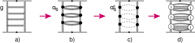
Figure 4: Multi-peripheral (ladder) diagrams contributing to the leading order BFKL Pomeron(Fig. 4-a) and to the soft Pomeron (Fig. 4-b - Fig. 4-d). The helical lines describe the gluons, the dashed lines correspond to pions. Fig. 4-d shows the contribution of the QCD instantons to the soft Pomeron structure.

The disappearance of the coupling constant in the spectral density of the $g^{2}F^{2}$ operator can be explained, if we assume, that non-perturbative QCD vacuum is dominated by the semi–classical fluctuations of the gluon field. Since the strength of the classical gluon field is inversely proportional to the coupling, $F\sim 1/g$, the quark zero modes, and the spectral density of their pionic excitations, appear independent of the coupling constant. Summing the ladder diagrams of Fig. 4-c we obtain the soft Pomeron with the intercept:

$$\Delta\,\,=\,\,\frac{1}{48}\,\,\ln\,\frac{M^{2}_{0}}{4m^{2}_{\pi}}\,\,.$$ (68)

In Ref.KKL the particular type of these classical fields are considered: we will assume, that the field is given by the instanton solution. It is shown, that these fields lead to the soft Pomeron (see ladder diagram of Fig. 4-d). The new dimensional scale in this particular approach is the typical size ($\rho_{0}$) of the instanton, which comes from the lattice calculation ($\rho_{0}\sim 0.3fm$). Summing the diagrams of Fig. 4-d we obtain the soft Pomeron contribution with the trajectory

$$\alpha\left(Q_{T}\right)\,\,=\,\,1\,\,+\,\,\Delta_{I\!\!P}\,\,-\,\,\alpha^{\prime}_{I\!\!P}\,Q^{2}_{T}$$ (69)

with $\Delta_{I\!\!P}\approx 0.08$ and $\alpha^{\prime}_{I\!\!P}\approx 0.25\,GeV^{-2}$. In Fig. 5 we plot the scales of QCD as they stem from our approach to the soft Pomeron of Eq. (69).

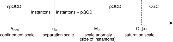
Figure 5: Scales of QCD.

Bearing in mind the hierarchy of the scales shown in Fig. 5, one can see, that the equation for the resulting Pomeron Green function takes the formBLT (see Fig. 6-a)

$$G\left(\omega,\boldsymbol{r}_{f},\boldsymbol{r}_{i},\boldsymbol{Q}_{T}\right)\,\,=$$ (70)

$$\,\,G^{0}\left(\omega,\boldsymbol{r}_{f},\boldsymbol{r}_{i},\boldsymbol{Q}_{T}\right)\,\,+\,\,\int d^{2}r^{\prime}\,d^{2}r"\,G^{0}\left(\omega,\boldsymbol{r}_{f},\boldsymbol{r}^{\prime},\boldsymbol{Q}_{T}\right)\Bigg{\{}K^{S}\left(\boldsymbol{r}^{\prime},\boldsymbol{r}",Q_{T}\right)\,+\,K^{\rm BFKL}\left(\boldsymbol{r}^{\prime},\boldsymbol{r}"\right)\Bigg{\}}G\left(\omega,\boldsymbol{r}",\boldsymbol{r}_{i},\boldsymbol{Q}_{T}\right)$$ (71)

In Eq. (70) $K^{\rm BFKL}\left(\boldsymbol{r}^{\prime},\boldsymbol{r}"\right)$ is familiar kernel of the BFKL equation (see Eq. (30)), while $K^{S}$ denotes the kernel of the soft Pomeron which we take in the form:

$$K^{S}\left(\boldsymbol{r}^{\prime},\boldsymbol{r}",Q_{T}\right)\,\,=\,\,\Delta\left(Q_{T}\right)\,D\left(r^{\prime}\right)\,D\left(r"\right)$$ (72)

with $\Delta\left(Q_{T}\right)\,\,=\,\,\Delta_{I\!\!P}\,\,-\,\,\alpha^{\prime}_{I\!\!P}\,Q^{2}_{T}$(see Eq. (69) ) and $D\left(r\right)$ is the function, which decreases with $r$ for $r>r_{\rm soft}=1/M_{0}$, where $M_{0}\,\approx 2\,GeV$, as we have discussed above. In addition we normalize $\int d^{2}r\,D\left(r\right)\,=\,1$.

Figure 6: Equation for the Pomeron Green function $G\left(\omega,\xi,Q_{T}\right)$( wavy lines in Fig. 6-a). $G^{0}\left(\omega,\xi,Q_{T}\right)$ denotes the Green function for the exchange of two gluons while $G^{H}\left(\omega,\xi,Q_{T}\right)$ is the Green function of the BFKL Pomeron.Fig. 6-b illustrates the solution of Eq. (73).

The solution to this equation, which is clear from Fig. 6-b, has the form (see appendix B of Ref.BLT ):

$$G\left(\omega,\boldsymbol{r}_{f},\boldsymbol{r}_{i},\boldsymbol{Q}_{T}\right)\,=$$ (73)

$$\,G^{H}\left(\omega,\boldsymbol{r}_{f},\boldsymbol{r}_{i},\boldsymbol{Q}_{T}\right)\,+\,\Delta\left(Q_{T}\right)\frac{\int d^{2}r^{\prime}D\left(r^{\prime}\right)G^{H}\left(\omega,\boldsymbol{r}_{f},\boldsymbol{r}^{\prime},\boldsymbol{Q}_{T}\right)\,\int d^{2}r"D\left(r"\right)G^{H}\left(\omega,\boldsymbol{r}",\boldsymbol{r}_{i},\boldsymbol{Q}_{T}\right)}{1\,-\,\Delta\left(Q_{T}\right)\int\int d^{2}r^{\prime}\,d^{2}r"\,D\left(r^{\prime}\right)\,G^{H}\left(\omega,\boldsymbol{r}^{\prime},\boldsymbol{r}",\boldsymbol{Q}_{T}\right)\,D\left(r"\right)}$$

The new singularities of the Green function stem from the equation:

$$1\,-\,\Delta\left(Q_{T}\right)\int\int d^{2}r^{\prime}\,d^{2}r"\,D\left(r^{\prime}\right)\,G^{H}\left(\omega,\boldsymbol{r}^{\prime},\boldsymbol{r}",\boldsymbol{Q}_{T}\right)\,D\left(r"\right)\,\,=\,\,0$$ (74)

Integrals over $r^{\prime}$ and $r"$ lead to $r^{\prime}=r^{\prime\prime}\approx r_{\rm soft}$, and the Green function of the BFKL Pomeron (see Eq. (36) and Eq. (37)) is equal to $\frac{1}{2\sqrt{D\left(\omega-\omega_{0}\right)}}$ . Therefore, Eq. (74) reduces to

$$4\,D\left(\omega-\omega_{0}\right)=\Delta^{2}\left(Q_{T}\right)~{}~{}~{}~{}~{}~{}~{}~{}~{}\mbox{or}~{}~{}~{}\omega=\omega_{0}+\frac{\Delta^{2}\left(Q_{T}\right)}{4\,D}\,=\,\frac{\Delta^{2}_{I\!\!P}}{4\,D}\,-\,\frac{\alpha^{\prime}_{I\!\!P}}{2D}\,\Delta_{{I\!\!P}}\,Q^{2}_{T}$$ (75)

From Eq. (75) we see, that the resulting intercept increases, which means that the soft Pomeron influences the energy behaviour of the deep inelastic processes. However, for this paper the most significant result is the impact parameter behaviour of the Green function.

Function $G_{I\!\!P}\left(\omega,Q_{T};r_{1},r_{2}\right)$ has been found in Ref.LIP , and it takes the following form (see Eq.35 in Ref.LIP )

$$G_{I\!\!P}\left(\omega,Q_{T};r_{1},r_{2}\right)\Big{|}_{\begin{minipage}{42.67912pt}{$\omega\to\omega_{0}\\ Q_{T}\to 0$ }\end{minipage}}\,\,=\,\,\,\frac{\pi}{\kappa_{0}}\Bigg{\{}\left(\frac{r_{1}}{r_{2}}\right)^{\kappa_{0}}\,\,+\,\,\left(\frac{r_{2}}{r_{1}}\right)^{\kappa_{0}}\,\,-\,\,2\,\left(Q^{2}_{T}\,r_{1}\,r_{2}\right)^{\kappa_{0}}\Bigg{\}}$$ (76)

From Eq. (76) one can see, that in the kinematic region of small $Q_{T}$ ,where $|(\omega-\omega_{0})\,\ln^{2}\left(Q^{2}_{T}r_{1}r_{2}\right)|\,\gg\,1$ $G_{I\!\!P}\left(\omega,Q_{T};r_{1},r_{2}\right)\,\,\to\,\,1/\sqrt{\omega-\omega_{0}}$ ( see section II-B-3), while in the region of $|(\omega-\omega_{0})\,\ln^{2}\left(Q^{2}_{T}r_{1}r_{2}\right)|\,\sim\,1$, $G_{I\!\!P}$ is less singular ($G_{I\!\!P}\left(\omega,Q_{T};r_{1},r_{2}\right)\,\,\to\,\,\sqrt{\omega-\omega_{0}}$. We will restrict ourselves to the region of small $Q_{T}$, since we are interested in the large impact parameter dependence of the Green function.

It can be estimated from the second term of Eq. (73), which takes the form

$$G\left(Y,\boldsymbol{r}_{f},\boldsymbol{r}_{i},\boldsymbol{b}\right)\, = \,\int^{\epsilon+i\infty}_{\epsilon-i\infty}\frac{d\omega}{2\,\pi\,i}\int\frac{d^{2}Q_{T}}{4\,\pi^{2}}e^{\omega_{0}\,Y+\delta\omega Y\,+\,\kappa_{0}\left(\xi_{f}+\xi_{i}\right)\,\,+\,\,\,i\boldsymbol{Q}_{T}\cdot\boldsymbol{b}}\,\frac{1}{2\sqrt{D\,\delta\omega}-\Delta_{I\!\!P}+\alpha^{\prime}_{I\!\!P}Q^{2}_{T}}\,$$ (77)

$$= \,\int^{\epsilon+i\infty}_{\epsilon-i\infty}\frac{d\omega}{2\,\pi\,i}\frac{1}{2\,\pi}e^{\omega_{0}Y\,+\,\kappa_{0}\left(\xi_{f}+\xi_{i}\right)}e^{\delta\omega\,Y}\,K_{0}\left(b\,\sqrt{\frac{\sqrt{\delta\omega}-\tilde{\Delta}_{I\!\!P}}{4\,\alpha^{\prime}_{I\!\!P}\,D}}\right)$$

where $\xi_{f}\,=\,\ln\left(r^{2}_{f}/r^{2}_{\rm soft}\right)$ and $\xi_{i}\,=\,\ln\left(r^{2}_{i}/r^{2}_{\rm soft}\right)$, $\delta\omega=\omega-\omega_{0}$, $\tilde{\Delta}_{I\!\!P}=\Delta_{I\!\!P}/\sqrt{4D}$ and $\kappa_{0}=\sqrt{\delta\omega/D}$.

Introducing a new variable $t=\sqrt{\delta\omega}-\Delta_{I\!\!P}$ we can re-write Eq. (77) in the form:

$$G\left(Y,\boldsymbol{r}_{f},\boldsymbol{r}_{i},\boldsymbol{b}\right)\, = \,\int^{\epsilon+i\infty}_{\epsilon-i\infty}\frac{2(t+\Delta_{I\!\!P})\,dt}{2\,\pi\,i}e^{\omega_{0}\,Y}\exp\left(\left(t+\tilde{\Delta}_{I\!\!P}\right)^{2}\,Y\,\,+\,\,\frac{t+\tilde{\Delta}_{I\!\!P}}{\sqrt{D}}\left(\xi_{f}+\xi_{i}\right)\,\,-\,\,b\,\sqrt{\frac{t}{\sqrt{4\,\alpha^{\prime 2}_{I\!\!P}\,D}}}\,\,\right)$$ (78)

$$= \,\int^{\epsilon+i\infty}_{\epsilon-i\infty}\frac{2(t+\tilde{\Delta}_{I\!\!P})\,dt}{2\,\pi\,i}e^{\omega_{0}\,Y}\exp\left(\left(t+\tilde{\Delta}_{I\!\!P}\right)^{2}\,Y\,\,+\,\,\left(t+\tilde{\Delta}_{I\!\!P}\right)\left(\tilde{\xi}_{f}+\tilde{\xi}_{i}\right)\,\,-\,\,b\,\sqrt{\frac{t}{\tilde{\alpha}^{\prime}_{I\!\!P}}}\,\,\right)$$

where $\tilde{\xi}_{i}=\xi/\sqrt{D}$ and $\tilde{\alpha}^{\prime}_{I\!\!P}=2\sqrt{D}\alpha^{\prime}_{I\!\!P}$.

Taking the integral of Eq. (78) using the method of steepest descent, we obtain the following equation for the saddle point value:

$$2\left(t_{SP}\,+\,\tilde{\Delta}_{I\!\!P}\right)\,Y\,\,+\,\,\left(\tilde{\xi}_{f}+\tilde{\xi}_{i}\right)\,\,-\,\,\frac{b}{2\sqrt{t_{SP}\,\tilde{\alpha}^{\prime}_{I\!\!P}}}\,\,=\,\,0$$ (79)

For large $b$ : $\frac{b}{2\sqrt{t_{SP}\,\tilde{\alpha}^{\prime}_{I\!\!P}}}\,\gg\,\left(\tilde{\xi}_{f}+\tilde{\xi}_{i}\right)$, and $t_{SP}\gg\tilde{\Delta}_{I\!\!P}$ the solution to Eq. (79) is $t=t_{SP}=\left(\frac{b}{4\sqrt{\tilde{\alpha}^{\prime}_{I\!\!P}}\,\,Y}\right)^{2/3}$.

Substituting $t_{SP}$ into the conditions for large $b$ we obtain:

$$\frac{b}{\sqrt{\tilde{\alpha}^{\prime}_{I\!\!P}}}\,\gg\,\tilde{\Delta}^{3/2}_{I\!\!P}4\,Y;~{}~{}~{}~{}~{}~{}~{}~{}~{}\frac{b^{2}}{\tilde{\alpha}^{\prime}_{I\!\!P}}\,\gg\,2\frac{\left(\tilde{\xi}_{f}+\tilde{\xi}_{i}\right)^{3}}{Y}$$ (80)

Plugging this $t_{SP}$ into Eq. (78) one can see that

$$G\left(Y,\boldsymbol{r}_{f},\boldsymbol{r}_{i},\boldsymbol{b}\right)\,\,\propto\,\,\,$$ (81)

$$\exp\left(\left(\omega_{0}+\tilde{\Delta}^{2}_{I\!\!P}\right)\,Y\,\,+2\tilde{\Delta}_{I\!\!P}\,Y\,\left(\frac{b^{2}}{16\,\tilde{\alpha}^{\prime}_{I\!\!P}\,Y^{2}}\right)^{1/3}\,\,+\,\,\left(\left(\frac{b^{2}}{16\,\tilde{\alpha}^{\prime}_{I\!\!P}\,Y^{2}}\right)^{1/3}\,\,+\,\,\tilde{\Delta}_{I\!\!P}\right)\left(\xi_{f}+\xi_{i}\right)\,\,-\,\,\frac{3}{4}\left(\frac{b^{4}}{4\tilde{\alpha}^{\prime 2}_{I\!\!P}\,\,Y}\right)^{1/3}\right)$$

.

Two lessons that we can learn from Eq. (81): (i) the random walk in $b$ leads to $\left\langle b^{2}\right\rangle\,\,\propto\,\,2\tilde{\alpha}^{\prime}_{I\!\!P}\,\sqrt{Y}$ and (ii) that the eikonal unitarization leads to the Froissart disc with radius

$$R\,\,\propto\,\,\left(\omega_{0}+\tilde{\Delta}_{I\!\!P}^{2}+2\left(\frac{4}{3}\left(\omega_{0}+\tilde{\Delta}^{2}_{I\!\!P}\right)^{3/2}\right)\right)\,Y\,\,+\,\,\left(\left(\frac{4}{3}\left(\omega_{0}+\tilde{\Delta}^{2}_{I\!\!P}\right)\right)^{3/2}\,+\,\tilde{\Delta}_{I\!\!P}\right)\,\left(\xi_{f}+\xi_{i}\right).$$ (82)

One can see that Eq. (82) satisfy the conditions of Eq. (80). Note, that we obtain the value of $\left\langle b^{2}\right\rangle$ and the radius of the Froissart disc in accord with the general analysis in section II-B-4.

III.6 Summing pion loops

In Ref.LEPION a theoretical approach is proposed, which is based on the assumption, that the BFKL Pomeron, being perturbative in nature, takes into account rather short distances (say of the order of $1/m_{G}$, where $m_{G}$ is the mass of the lightest glueball); and the long distance contribution can be described by the exchange of pions ($1/2\mu\,\gg\,1/m_{G}$, where $\mu$ is the pion mass). Indeed, the proof of the Froissart theorem indicates, that the exponential fall-off at large $b$ is closely related to the contribution of the exchange of two lightest hadrons: 2 pions, in $t$-channel (see Fig. 7-a). Fig. 7-b demonstrates both the main idea and the practical method of our approach. The set of diagrams of Fig. 7 can be summed, using the following equation:

$$G_{I\!\!P}\left(\omega,Q_{T};R_{\pi},R_{\pi}\right)\,\,=\,\,G^{\rm BFKL}_{I\!\!P}\left(\omega,Q_{T};R_{\pi},R_{\pi}\right)\,\,\,+\,\,G^{\rm BFKL}_{I\!\!P}\left(\omega,Q_{T};R_{\pi},R_{\pi}\right)\,\Sigma\left(\omega,Q_{T}\right)G_{I\!\!P}\left(\omega,Q_{T};R_{\pi},R_{\pi}\right)$$ (83)

where $G_{I\!\!P}$ denotes the resulting Green’s function of the Pomeron with the pion loops for $r_{1}=r_{2}=R_{\pi}$ where $R_{\pi}$ is the size of the pion. $G^{\rm BFKL}_{I\!\!P}$ is the Green function of the BFKL Pomeron.

Fig. 7-a		Fig. 7-b

Figure 7: Fig. 7-a: The exchange of two pions, that gives the main contribution to the large $b$ behaviour of the scattering amplitudeFROI .Fig. 7-b:The diagrams that describe the pion loop contribution to the BFKL Pomeron. The wavy line describe the BFKL Pomeron, the dashed line stands for pion. The zigzag line denotes the resulting Pomeron.

$$G_{I\!\!P}\left(\omega,Q_{T};R_{\pi},R_{\pi}\right)\,\,=\,\,\frac{1}{G^{-1}_{I\!\!P}\left(\omega,Q_{T};R_{\pi},R_{\pi}\right)\,\,-\,\,\Sigma\left(\omega,Q_{T}\right)}$$ (84)

The $t$-channel unitarity for $G_{I\!\!P}\left(\omega,Q_{T};R_{\pi},R_{\pi}\right)$ is used to calculate $\Sigma$, as it was suggested in Ref.ANGR . The unitarity constraints for $G_{I\!\!P}$ takes the form COL ; GRLEC ($t=-Q^{2}_{T}$):

$$-i\{G_{I\!\!P}\left(\omega,t+i\epsilon;R_{\pi},R_{\pi}\right)\,\,-\,\,G_{I\!\!P}\left(\omega,t-i\epsilon;R_{\pi},R_{\pi}\right)\}\,\,=\,\,\rho\left(\omega,t\right)G_{I\!\!P}\left(\omega,t+i\epsilon;R_{\pi},R_{\pi}\right)\,G_{I\!\!P}\left(\omega,t-i\epsilon;R_{\pi},R_{\pi}\right)$$ (85)

Eq. (85) is written for $t\,>\,4\mu^{2}$ where $\mu$ is the mass of pion. We wish to only sum the two pion contribution, assuming that all other have been taken into account in the BFKL Pomeron. In other words, we believe that Eq. (85) can be trusted for $t\,<\,m^{2}_{G}$ where $m_{G}$ is the lightest glueball. $\rho\left(\omega,t\right)$ is equal to $(t-4\mu^{2})^{\frac{3}{2}+\omega}/\sqrt{t}$. Plugging in Eq. (85) the solution of Eq. (84) we obtain the following equation for $\Sigma$:

$$\mbox{Im}_{t}\Sigma\left(\omega,t\right)\,\,=\,\,\frac{1}{2}\rho\left(\omega,t\right)\,\Big{(}\Gamma^{I\!\!P}_{\pi\pi}\Big{)}^{2}\,\frac{1}{\omega+2}$$ (86)

where vertex $\Gamma^{I\!\!P}_{\pi\pi}$ describes the interaction of the BFKL Pomeron with $\pi$-meson and it has been evaluated in Ref.LEPION : $\Gamma^{I\!\!P}_{\pi\pi}\,\,=\,\,=\,\,\frac{8}{9}\,\bar{\alpha}_{S}\,R_{\pi}$. Experimentally $<R^{2}_{\pi}>=0.438\pm 0.008\,fm^{2}$ PIR and we will bear this value in mind for the numerical estimates.

We use dispersion relations to calculate $\Sigma$. Since we believe, that non-perturbative corrections will not change the intercept of the BFKL Pomeron (see Refs.LETA ; LLS ) we write the dispersion relation with one subtraction. It takes the form

$$\Sigma\left(\omega,t\right)\,\,=\,\,t\,\frac{1}{\pi}\int\frac{dt^{\prime}\,\mbox{Im}_{t}\Sigma\left(\omega,t^{\prime}\right)}{t^{\prime}\,(t^{\prime}-t)}\,\,=\,\,t\frac{3}{2}\,\frac{1}{\omega+2}\frac{\left(\Gamma^{I\!\!P}_{\pi\pi}\right)^{2}}{\pi}\int_{4\mu^{2}}^{m_{G}^{2}}\frac{dt^{\prime}\,\rho\left(\omega,t^{\prime}\right)}{t^{\prime}\,(t^{\prime}-t)}\,\,=\,\,\bar{\alpha}_{S}^{2}\,\frac{16}{9}\,R^{2}_{\pi}\,\,\frac{1}{\omega+2}\,\,t\int_{4\mu^{2}}^{m_{G}^{2}}\,\frac{dt^{\prime}\,\rho\left(\omega,t^{\prime}\right)}{t^{\prime}\,(t^{\prime}-t)}$$ (87)

Factor $3/2$ stems from two states in $t$-channel: $\pi^{+}\,\pi^{-}$ and $\pi^{0}\,\pi^{0}$. The integral over $t^{\prime}$ for $\omega\,\ll\,1$ has been taken in Ref.ANGR . For fixed $\omega$

$$\Sigma\left(\omega,Q_{T}\right)\,\,\,=\,\,\,\bar{\alpha}_{S}^{2}\,\frac{16}{9}\,R^{2}_{\pi}\,\,\frac{1}{\omega+2}\,\,(-Q^{2}_{T})\,\frac{\left(m^{2}_{G}\right)^{5/2+\omega}}{8\mu^{2}*\left(5+2\omega\right)\left(4\mu^{2}+Q^{2}_{T}\right)}\,F_{1}\left(\frac{5}{2}+\omega,\frac{3}{2},1,\frac{7}{2}+\omega,-\frac{m^{2}_{G}}{4\mu^{2}},-\frac{m^{2}_{G}}{4\mu^{2}+Q^{2}_{T}}\right)$$ (88)

where $F_{1}$ is the Appell $F_{1}$ function ( see Ref.RY formulae 9.180 - 9.184).

The linear term in $Q^{2}_{T}$ can be easily found since two arguments in $F_{1}$ coincide, and we can use the relation (see Ref.RY formula 9.182(11)) and reduce Eq. (88) to the form

$$\Sigma\left(\omega,Q_{T}\right)\,\,\,=\,\,\,\bar{\alpha}_{S}^{2}\,\frac{16}{9}\,R^{2}_{\pi}\,\,\frac{1}{\omega+2}\,\,(-Q^{2}_{T})\,\frac{\left(m^{2}_{G}\right)^{5/2+\omega}}{8\mu^{2}*\left(5+2\omega\right)\left(4\mu^{2}+Q^{2}_{T}\right)}\,{}_{2}F_{1}\left(\frac{5}{2}+\omega,\frac{5}{2},\frac{7}{2}+\omega,-\frac{m^{2}_{G}}{4\mu^{2}}\right)$$ (89)

For $m_{G}\,\gg\,\mu$ Eq. (89) takes the form

$$\Sigma\left(\omega,Q_{T}\right) = \,\,\,\bar{\alpha}_{S}^{2}\,\frac{16}{9}\,R^{2}_{\pi}\,\,\frac{1}{\omega+2}\,\,(-Q^{2}_{T})$$

$$\times \Bigg{\{}\frac{1}{\sqrt{\pi}\,3\left(5+2\omega\right)}4^{1+\omega}\left(\frac{1}{\mu^{2}}\right)^{\frac{1}{2}+\omega}\!\!\!\!\!\!\mu\,\left(2+3\omega+\omega^{3}\right)\Gamma\left(-2-\omega\right)\Gamma\left(\frac{7}{2}+\omega\right)\,+\,\frac{\left(m^{2}_{G}\right)^{\omega}}{\omega}\,\frac{4+2\omega+3\omega^{2}+\omega^{3}}{4(2+\omega)}\Bigg{\}}$$

$$= -Q^{2}_{T}\,\alpha^{\prime}_{eff}\left(\bar{\alpha}_{S}\right)$$

We evaluate $\alpha^{\prime}_{eff}\left(\bar{\alpha}_{S}\right)$ using $R^{2}_{\pi}=0.436fm^{2}$ and the value for $m^{2}_{G}=5\,GeV^{2}$ that stems from lattice calculation of the glueball masses GLUETR for the Pomeron trajectory. In principle we can consider this coefficient as the only non-perturbative input that we need, but it is pleasant to realize that simple estimates give a sizable value of $0.1\,GeV^{-2}$ for $\bar{\alpha}_{S}\ =0.3$ (see Ref.LEPION ).

Comparing Eq. (84) with Eq. (77) we see that the difference is only that in Eq. (84) we put $\Delta_{I\!\!P}=0$, and the new dimensional scale is determined by the mass of the lightest glueball $m_{G}$. Bearing this in mind and using Eq. (81) we obtain:

$$G\left(Y,\boldsymbol{r}_{f},\boldsymbol{r}_{i},\boldsymbol{b}\right)\,\,\propto\,\,\,\exp\left(\omega_{0}\,Y\,+\,\,\left(\frac{b^{2}}{16\,\tilde{\alpha}^{\prime}_{I\!\!P}\,Y^{2}}\right)^{1/3}\left(\tilde{\xi}_{f}+\tilde{\xi}_{i}\right)\,\,-\,\,\frac{3}{4}\left(\frac{b^{4}}{4\tilde{\alpha}^{\prime 2}_{I\!\!P}\,\,Y}\right)^{1/3}\right)$$ (91)

with $r_{\rm soft}=1/m_{G}$.

In Eq. (91) we replace Eq. (83) by a more general Eq. (70) with the solution of Eq. (73). We believe that Eq. (73) gives the solution to the problem of large $b$ behaviour.

As we have mentioned, obtaining this equation we used, based on the results of Refs.LETA ; LLS , that the non-perturbative corrections do not change the intercept of the BFKL Pomeron. One way to check this key assumption is to try to describe the experimental data for the soft interaction at high energy, assuming, that we have only the BFKL Pomeron. In Refs.GLP the model for the soft interaction was built, which based on two main ingredients: (i) CGC approach for the scattering amplitude of two dipoles; and (ii) phenomenological description of the hadron structure. In this model, we successfully describe the DIS data from HERA, the total, inelastic, elastic and diffractive cross sections, the t-dependence of these cross sections, as well as the inclusive production and rapidity and angular correlations in a wide range of energies, including that of the LHC.

III.7 Resume

Concluding this brief review, we believe, that Eq. (91) incorporates correctly the QCD random walk in the impact parameters ($b$) into the BFKL equation. We would like to emphasize, that two main ingredients formed the basis of this conclusion: the assumption, that the non-perturbative modification of the BFKL Pomeron does not change its intercept; and our result of section II-B-4, that $\left\langle b^{2}\right\rangle$ for the QCD diffusion in $b$ is proportional to $\sqrt{Y}$.

Insufficiency of Eq. (91) is, that it gives the modification of the Green function of the perturbative BFKL Pomeron, but it is not written as an alternative for the non-linear Balitsky-Kovchegov equation. On the other hand, for discussion of the asymptotic behaviour of the scattering amplitude at high energy, we need a new evolution equation, which will include on the same footing both the shadowing corrections, and the correct behaviour at large impact parameter.

IV A new non-linear evolution equation

We proposed the following generalization of the Balitsky-Kovchegov non-linear evolution equation:

$$\frac{\partial}{\partial Y}N\left(\boldsymbol{r},\boldsymbol{b},Y\right) = \bar{\alpha}_{S}\!\!\int\frac{d^{2}\boldsymbol{r}^{\prime}}{2\,\pi}\,K\left(\boldsymbol{r}^{\prime},\boldsymbol{r}-\boldsymbol{r}^{\prime};\boldsymbol{r}\right)\Bigg{\{}N\left(\boldsymbol{r}^{\prime},\boldsymbol{b}-\frac{1}{2}\left(\boldsymbol{r}-\boldsymbol{r}^{\prime}\right),Y\right)+N\left(\boldsymbol{r}-\boldsymbol{r}^{\prime},\boldsymbol{b}-\frac{1}{2}\boldsymbol{r}^{\prime},Y\right)\,\,-\,\,N\left(\boldsymbol{r},\boldsymbol{b},Y\right)$$

$$~{}~{}~{}~{}~{}~{}~{}-N\left(\boldsymbol{r}-\boldsymbol{r}^{\prime},\boldsymbol{b}-\frac{1}{2}\boldsymbol{r}^{\prime},Y\right)\,N\left(\boldsymbol{r}^{\prime},\boldsymbol{b}-\frac{1}{2}\left(\boldsymbol{r}-\boldsymbol{r}^{\prime}\right),Y\right)\Bigg{\}}\,\,\,+\,\,\,\left(\alpha^{\prime}_{\rm eff}\,\nabla^{2}_{b}\right)^{2}\,N\left(\boldsymbol{r},\boldsymbol{b},Y\right)$$

$$\xrightarrow{b\gg r,r^{\prime}} \bar{\alpha}_{S}\!\!\int\frac{d^{2}\boldsymbol{r}^{\prime}}{2\,\pi}\,K\left(\boldsymbol{r}^{\prime},\boldsymbol{r}-\boldsymbol{r}^{\prime};\boldsymbol{r}\right)\Bigg{\{}N\left(\boldsymbol{r}^{\prime},\boldsymbol{b},Y\right)+N\left(\boldsymbol{r}-\boldsymbol{r}^{\prime},\boldsymbol{b},Y\right)\,\,-\,\,N\left(\boldsymbol{r},\boldsymbol{b},Y\right)$$

$$~{}~{}~{}~{}~{}~{}~{}~{}~{}~{}~{}-N\left(\boldsymbol{r}-\boldsymbol{r}^{\prime},\boldsymbol{b},Y\right)\,N\left(\boldsymbol{r}^{\prime},\boldsymbol{b},Y\right)\Bigg{\}}\,\,\,+\,\,\,\left(\alpha^{\prime}_{\rm eff}\,\nabla^{2}_{b}\right)^{2}\,N\left(\boldsymbol{r},\boldsymbol{b},Y\right)$$

Where $\alpha^{\prime}_{\rm eff}$ is a new dimensional scale. We believe that Eq. (IV) is the correct way to introduce this scale in the non-linear evolution.

IV.1 The BFKL Pomeron with diffusion in $b$

First, let us solve the new equation at large $b$, where only the linear part contributes. The equation takes the form:

$$\frac{\partial}{\partial Y}N\left(\boldsymbol{r},\boldsymbol{b},Y\right)=\bar{\alpha}_{S}\!\!\int\frac{d^{2}\boldsymbol{r}^{\prime}}{2\,\pi}\,K\left(\boldsymbol{r}^{\prime},\boldsymbol{r}-\boldsymbol{r}^{\prime};\boldsymbol{r}\right)\Bigg{\{}N\left(\boldsymbol{r}^{\prime},\boldsymbol{b},Y\right)+N\left(\boldsymbol{r}-\boldsymbol{r}^{\prime},\boldsymbol{b},Y\right)-N\left(\boldsymbol{r},\boldsymbol{b},Y\right)\Bigg{\}}\,\,\,+\,\,\,\left(\alpha^{\prime}_{\rm eff}\,\nabla^{2}_{b}\right)^{2}\,N\left(\boldsymbol{r},\boldsymbol{b},Y\right)$$ (92)

We can obtain the solution to this equation using it in the form: $N\left(\boldsymbol{r},\boldsymbol{b},Y\right)\,\,=\,\,G\left(\boldsymbol{r},Y\right)\,\Phi\left(Y;b\right)$ where $G\left(\boldsymbol{r},Y\right)$ is the Green’s function of the BFKL equation and $\Phi\left(Y;b\right)$ satisfies the following equation

$$\frac{\partial}{\partial Y}\Phi\left(\boldsymbol{b},Y\right)\,\,=\,\,\,\,\,\left(\alpha^{\prime}_{\rm eff}\,\nabla^{2}_{b}\right)^{2}\,\Phi\left(\boldsymbol{b},Y\right)$$ (93)

In $\omega$-representation:

$$\Phi\left(\boldsymbol{b},Y\right)\,\,=\,\,\int^{\epsilon+i\infty}_{\epsilon-i\infty}\frac{d\,\omega}{2\,\pi\,i}\,e^{\omega\,Y}\,\Phi\left(\boldsymbol{b},\omega\right)$$ (94)

Eq. (93) takes the form

$$\left(\alpha^{\prime}_{\rm eff}\,\nabla^{2}_{b}\right)^{2}\,\Phi\left(\boldsymbol{b},\omega\right)\,\,=\,\,\omega\,\Phi\left(\boldsymbol{b},\omega\right)$$ (95)

The general solution to Eq. (95) can be written (see Ref. MATH formula 9.4.3) as

$$\Phi\left(\boldsymbol{b},\omega\right)\,\,=\,\,\Phi_{-}\left(\boldsymbol{b},\omega\right)\,\,+\,\,\Phi_{+}\left(\boldsymbol{b},\omega\right)$$ (96)

where $\Phi_{\pm}$ are the solution to the following equations:

$$\alpha^{\prime}_{\rm eff}\,\nabla^{2}_{b}\,\Phi_{\pm}\left(\boldsymbol{b},\omega\right)\,\,\pm\,\,\sqrt{\omega}\,\Phi_{\pm}\left(\boldsymbol{b},\omega\right)\,\,=\,\,0$$ (97)

We restrict ourself by the solution $\Phi\left(\boldsymbol{b},\omega\right)\,\,=\,\,\,\Phi_{+}\left(\boldsymbol{b},\omega\right)$ for which the Green’s function is equal to

$$\Phi_{+}\left(\boldsymbol{b},\omega\right)\,\,=\,\,\int\frac{d^{2}Q_{T}}{(2\pi)^{2}}\,e^{i\boldsymbol{Q}_{T}\cdot\boldsymbol{b}}\frac{\phi^{in}_{+}\left(\omega\right)}{\alpha^{\prime}_{\rm eff}\,Q^{2}_{T}\,\,+\,\,\sqrt{\omega}}$$ (98)

where $\phi^{in}_{+}\left(\omega\right)$ should be found from the initial condition at $Y=0$. Searching for the Green’s function of Eq. (98) we impose the initial condition:

$$\Phi_{+}\left(\boldsymbol{b},Y=0\right)\,\,=\,\,\delta^{(2)}\left(\boldsymbol{b}\right)$$ (99)

which results in $\phi^{in}_{+}\left(\omega\right)\,\,=\,\,1/\left(2\sqrt{\omega}\right)$.

The similarities between this equation and Eq. (77) and Eq. (84) are obvious. Taking integral over $d^{2}Q_{T}$ we obtain:

$$\Phi_{+}\left(\boldsymbol{b},\omega\right)\,\,=\frac{1}{4\,\pi\,\alpha^{\prime}_{\rm eff}\,\sqrt{\omega}}K_{0}\left(\frac{b}{\sqrt{\alpha^{\prime}_{\rm eff}}}\,\omega^{1/4}\right)$$ (100)

and for $\Phi\left(\boldsymbol{b},Y\right)$ we have

$$\Phi\left(\boldsymbol{b},Y\right)\,\,=\,\,\,\int^{\epsilon+i\infty}_{\epsilon-i\infty}\frac{d\,\omega}{8\pi^{2}\,i}\,\frac{1}{\,\alpha^{\prime}_{\rm eff}\,\sqrt{\omega}}\,e^{\omega\,Y}\,K_{0}\left(\frac{b}{\sqrt{\alpha^{\prime}_{\rm eff}}}\,\omega^{1/4}\right)$$ (101)

For large $b$ we can take the integral over $\omega$ plugging the asymptotic behaviour of the $K_{0}$ function and using the method of steepest descend. Eq. (101) takes the form:

$$\Phi\left(\boldsymbol{b},Y\right)\,\,=\,\,\,\int^{\epsilon+i\infty}_{\epsilon-i\infty}\frac{d\,\omega}{8\pi^{2}\,i}\,\frac{1}{\alpha^{\prime}_{\rm eff}\,\sqrt{\omega}}\,e^{\omega\,Y}\,\sqrt{\frac{\pi}{2}}\left(\frac{1}{\omega}\right)^{1/8}\frac{1}{\sqrt{\frac{b}{\sqrt{\alpha^{\prime}_{\rm eff}}}}}\,e^{-\frac{b}{\sqrt{\alpha^{\prime}_{\rm eff}}}\,\omega^{1/4}}$$ (102)

The equation for the saddle point has the following form

$$Y\,\,-\,\,\frac{1}{4}\frac{\frac{b}{\sqrt{\alpha^{\prime}_{\rm eff}}}}{\omega^{3/4}_{\rm SP}}\,\,=\,\,0;~{}~{}~{}~{}~{}~{}~{}~{}~{}~{}~{}\omega_{\rm SP}\,\,=\,\,\Bigg{(}\frac{b}{4\,Y\,\sqrt{\alpha^{\prime}_{\rm eff}}}\Bigg{)}^{4/3};$$ (103)

From Eq. (103) we obtain for the integral over $\omega$:

$$\Phi\left(\boldsymbol{b},Y\right)\,\,=\,\,\frac{4\,\pi}{\sqrt{6}\,\alpha^{\prime}_{\rm eff}}\Bigg{(}\frac{\alpha^{\prime}_{\rm eff}}{4\,Y\,b^{2}}\Bigg{)}^{1/3}\,\exp\left(-\frac{3}{4}\,{\cal Z}\right)$$ (104)

where

$${\cal Z}\,=\,\left(\frac{b^{4}}{4{\alpha^{\prime}}^{2}_{\rm eff}\,Y}\right)^{1/3}$$ (105)

Finally, from $N\left(\boldsymbol{r},\boldsymbol{b},Y\right)\,\,=\,\,G\left(\boldsymbol{r},Y\right)\,\Phi\left(Y;b\right)$ we obtain

$$G\left(\boldsymbol{r},\boldsymbol{b},Y\right)\,\,=\,\,\int^{\epsilon+i\,\infty}_{\epsilon-i\,\infty}\frac{d\gamma}{2\,\pi\,i}e^{\bar{\alpha}_{S}\chi\left(\gamma\right)\,Y\,\,-\,\,\left(-\gamma\right)\xi}\,\Phi\left(Y;b\right)\,\,=\,\,\,\,\frac{r}{R}e^{\omega_{0}\,Y}\frac{1}{2\sqrt{\pi\,D\,Y}}\,\,e^{-\frac{\xi^{2}}{4\,D\,Y}}\,\Phi\left(Y;b\right)$$ (106)

and $\Phi\left(Y;b\right)$ is given by Eq. (104). In Eq. (106) we integrated over $\gamma$ using the diffusion expansion for the kernel, $\chi(\gamma)$ for $\gamma\to\frac{1}{2}$.

For the region of not large $b$ we obtain the solution which has a cumbersome form:

$$\frac{1}{16\,{\alpha^{\prime}}^{2}_{\rm eff}\,Y}\Bigg{(}-4\sqrt{\pi}\sqrt{-{\alpha^{\prime}}^{2}_{\rm eff}\,Y}\,\,_{0}F_{2}\left(;\frac{1}{2},1;-\,\frac{b^{4}}{256\,{\alpha^{\prime}}^{2}_{\rm eff}\,Y}\right)-b^{2}\,_{0}F_{2}\left(;\frac{3}{2},\frac{3}{2};-\,\frac{b^{4}}{256\,{\alpha^{\prime}}^{2}_{\rm eff}\,Y}\right)\Bigg{)}$$ (107)

where ${}_{0}F_{2}$ is the hyperbolic function (see formula 9.14 of Ref.RY ).

As we have mentioned above the solution of Eq. (104) is the Green’s function of Eq. (93), and it preserves the remarkable property of the Green’s function of the BFKL Pomeron:

$$\Phi\left(\boldsymbol{b},Y\right)\,\, = \,\,\int\,d^{2}b^{\prime}\,\Phi\left(\boldsymbol{b}-\boldsymbol{b}^{\prime},Y-Y^{\prime}\right)\,\,\Phi\left(\boldsymbol{b}^{\prime},Y^{\prime}\right)\,\,$$ (108)

$$= \,\,\,\int\,d^{2}b^{\prime}\int\frac{d^{2}Q^{\prime}_{T}}{4\pi^{2}}\exp\Bigg{(}\,\,{\alpha^{\prime}}^{2}_{\rm eff}\,Q^{\prime 4}_{T}\,Y^{\prime}\,\,+i\boldsymbol{Q^{\prime}}_{T}\cdot\boldsymbol{b}^{\prime}\Bigg{)}\,\int\frac{d^{2}Q_{T}}{4\pi^{2}}\exp\Bigg{(}\,\,{\alpha^{\prime}}^{2}_{\rm eff}\,Q^{4}_{T}\,\left(Y\,-\,Y^{\prime}\right)+i\,\boldsymbol{Q}_{T}\cdot\left(\boldsymbol{b}-\boldsymbol{b}^{\prime}\right)\Bigg{)}$$ (109)

$$= \,\,\int d^{2}Q_{T}\exp\Big{(}{\alpha^{\prime}}^{2}_{\rm eff}\,Q^{\prime 4}_{T}\,\,+\,\,i\,\boldsymbol{Q^{\prime}}_{T}\cdot\boldsymbol{b}\Big{)}$$

In Eq. (108) we use Eq. (98) for $\Phi_{+}\left(\boldsymbol{b},\omega\right)$ which leads to the following representation for $\Phi\left(\boldsymbol{b},Y\right)$

$$\Phi\left(\boldsymbol{b},Y\right)\,\,=\,\,\int^{\epsilon+i\,\infty}_{\epsilon-i\,\infty}\frac{d\omega}{2\,\pi\,i}\,e^{\omega\,Y}\,\Phi_{+}\left(\boldsymbol{b},\omega\right)\,\,=\,\,\int d^{2}Q_{T}\exp\Big{(}{\alpha^{\prime}}^{2}_{\rm eff}\,Q^{\prime 4}_{T}\,\,+\,\,i\,\boldsymbol{Q^{\prime}}_{T}\cdot\boldsymbol{b}\Big{)}$$ (110)

One can see, that the integration over $d^{2}b^{\prime}$ in Eq. (108) generates $\delta{(2)}\left(\boldsymbol{Q}_{T}-\boldsymbol{Q}^{\prime}_{T}\right)$, which results in Eq. (108).

Using Eq. (108) we can prove that for the Green’s function of Eq. (106) we have the following equation:

$$G\left(\boldsymbol{r},\boldsymbol{b},\boldsymbol{R},Y\right)\,\, = \,\,\int d^{2}r^{\prime}\,d^{2}b^{\prime}\,G\left(\boldsymbol{r},\boldsymbol{b}-\boldsymbol{b}^{\prime},\boldsymbol{r}^{\prime},Y-Y^{\prime}\right)\,\,G\left(\boldsymbol{r}^{\prime},\boldsymbol{b}^{\prime},\boldsymbol{R},Y^{\prime}\right)\,\,$$ (111)

$$= \,\,\,\int d\xi^{\prime}\,d^{2}b^{\prime}\int\frac{d\gamma^{\prime}}{2\,\pi\,i}\int\frac{d^{2}Q^{\prime}_{T}}{4\pi^{2}}\exp\Bigg{(}\left(\bar{\alpha}_{S}\chi\left(\gamma^{\prime}\right)\,\,+\,\,{\alpha^{\prime}}^{2}_{\rm eff}\,Q^{\prime 4}_{T}\right)\,Y^{\prime}\,+\,\left(\gamma^{\prime}-1\right)\,\xi^{\prime}+i\boldsymbol{Q^{\prime}}_{T}\cdot\boldsymbol{b}^{\prime}\Bigg{)}$$

$$\times \,\int\frac{d\gamma}{2\,\pi\,i}\int\frac{d^{2}Q_{T}}{4\pi^{2}}\exp\Bigg{(}\left(\bar{\alpha}_{S}\chi\left(\gamma\right)\,\,+\,\,{\alpha^{\prime}}^{2}_{\rm eff}\,Q^{4}_{T}\right)\,\left(Y\,-\,Y^{\prime}\right)\,+\,\left(\gamma-1\right)\left(\xi-\xi^{\prime}\right)+i\boldsymbol{Q}_{T}\cdot\left(\boldsymbol{b}-\boldsymbol{b}^{\prime}\right)\Bigg{)}$$

where $\xi^{\prime}\,=\,\ln\left(r^{\prime 2}/R^{2}\right)$.

The integration over $\xi^{\prime}$ and $\boldsymbol{b}^{\prime}$ gives $\delta\left(\gamma-\gamma^{\prime}\right)$ and $\delta^{(2)}\left(\boldsymbol{Q}_{T}\,-\,\boldsymbol{Q}^{\prime}_{T}\right)$ , which leads to tequation Eq. (111).

One can see that Eq. (106) has the same main features as Eq. (91). In particular, the unitaristion leads to the Froissart disc with radius

$$\frac{R}{\sqrt{{\alpha^{\prime}}_{\rm eff}}}\,\,=\,\,\frac{4}{3^{3/4}}\,\omega_{0}^{3/4}\,Y\,\,\,-\,\,\frac{3^{1/4}}{4\,D\,\omega^{1/4}_{0}}\frac{\xi^{2}}{Y}$$ (112)

whose edge decreases with $b$ as $e^{-\frac{3}{4}\left(\frac{b^{4}}{4{\alpha^{\prime}}^{2}_{\rm eff}\,Y}\right)^{1/3}}$ which corresponds to the diffusion in $b$ with $\left\langle b^{2}\right\rangle\propto\sqrt{Y}$, as follows from section II-B-4.

IV.2 Solution in the vicinity of the saturation scale

The behaviour of the scattering dipole amplitude in the vicinity of the saturation scale can be found from the solution of the linear equationGLR ; MUT . We will use the solution to Eq. (92) in the form of Eq. (104), and will take the integral over $\gamma$ using the method of steepest descend. The equation for the saddle point in $\gamma$ has the form:

$$\bar{\alpha}_{S}\frac{d\chi\left(\gamma\right)}{d\gamma}\Bigg{|}_{\gamma=\gamma_{\rm SP}}\,Y\,\,+\,\,\xi\,\,=\,\,0$$ (113)

The second condition is that the scattering amplitude is a constant for $r^{2}\,Q^{2}_{s}=1$, which has the form

$$\bar{\alpha}_{S}\,\chi\left(\gamma_{\rm SP}\right)\,Y\,\,+\,\,\left(\gamma_{\rm SP}\,-\,1\right)\xi\,\,-\,\,\frac{3}{4}{\cal Z}\,\,=\,\,0$$ (114)

Plugging Eq. (113) into Eq. (114) we obtain the following equation for $\gamma_{\rm SP}$.

$$\bar{\alpha}_{S}\left(\chi\left(\gamma_{\rm SP}\right)\,\,+\,\,\left(1-\gamma_{\rm SP}\right)\,\frac{d\chi\left(\gamma\right)}{d\gamma}\Big{|}_{\gamma=\gamma_{\rm SP}}\right)\,Y\,\,=\,\,\frac{3}{4}{\cal Z}$$ (115)

For ${\cal Z}=0$ the solution to Eq. (115) is $\gamma_{\rm SP}=\gamma_{cr}\approx 0.37$. If ${\cal Z}\,\ll\bar{\alpha}_{S}\,\,Y$ we can find the solution to Eq. (115) assuming, that $\gamma_{\rm SP}\,=\,\gamma_{cr}\,+\,\delta\gamma$ with $\delta\gamma\,\ll\,\gamma_{cr}$. The value of $\delta\gamma$ from Eq. (115) turns out to be equal to

$$\delta\gamma\,\,=\,\,\frac{3}{4}\frac{1}{\left(1-\gamma_{cr}\right)\,\frac{d\chi\left(\gamma\right)}{d\gamma}\Big{|}_{\gamma=\gamma_{cr}}}\,\frac{\cal Z}{\bar{\alpha}_{S}\,Y}$$ (116)

Substituting $\gamma_{\rm SP}\,=\,\gamma_{cr}\,+\,\delta\gamma$ into Eq. (113) we obtain the expression for the saturation momentum:

$$\xi_{s}\,=\,\ln\left(Q^{2}_{s}\right)\,\,=\,\,\bar{\alpha}_{S}\frac{\chi\left(\gamma_{cr}\right)}{1-\gamma_{cr}}\,Y\,\,-\,\frac{3}{4\left(1-\gamma_{cr}\right)}{\cal Z}$$ (117)

In the vicinity of the saturation scale the scattering amplitude shows geometric scaling behaviourGS1 ; LETU ; GS2 ; GS3 and has the following form MUT for $\tau\sim 1$:

$$N\left(r,b,Y\right)\,\,=\,\,N_{0}\left(r^{2}\,Q^{2}_{s}\left(Y,b\right)\right)^{1-\gamma_{cr}}\,=\,N_{0}\tau^{1-\gamma_{cr}}$$ (118)

where $N_{0}$ is a constant and we assumed that $\delta\gamma\,\ln\tau\,\ll\,1$.

Using Eq. (117) for $Q_{s}$ we see that $N\left(r,b,Y\right)$ of Eq. (118) can be re-written in the form:

$$N\left(r,b,Y\right)\,\,=\,\,N_{0}\left(r^{2}\,Q^{2}_{s}\left(Y,b=0\right)\right)^{1-\gamma_{cr}}\,e^{-\frac{3}{4}\left(\frac{b^{4}}{4{\alpha^{\prime}}^{2}_{\rm eff}\,Y}\right)^{1/3}}$$ (119)

for the kinematic region

$$r^{2}\,Q^{2}_{s}\left(Y=0\right)e^{\bar{\alpha}_{S}\frac{\chi\left(\gamma_{cr}\right)}{1-\gamma_{cr}}\,Y\,\,-\,\frac{3}{4\left(1-\gamma_{cr}\right)}{\cal Z}}\,\,\sim\,\,1$$ (120)

IV.3 The scattering amplitude in the deep saturation region

We use the approach of Ref.LETU for linearizing Eq. (IV) deep inside the saturation region ($r^{2}\,Q^{2}_{s}\left(Y,b\right)\,\gg\,1$): we assume that $N\left(r,b,Y\right)\,\to\,1$ and neglect the contributions, which are proportional to $\Delta^{2}\left(r,b,Y\right)\,\ll\,1$ where $N\left(r,b,Y\right)\,=\,1\,-\,\Delta\left(r,b,Y\right)$. Eq. (IV) reduces to the following linear equation for $\Delta\left(r,b,Y\right)$

$$\frac{\partial}{\partial Y}\Delta\left(\boldsymbol{r},\boldsymbol{b},Y\right)\,\,=\,\,\,-\bar{\alpha}_{S}\!\!\int^{r}_{1/Q_{s}\left(Y,b\right)}\frac{d^{2}\boldsymbol{r}^{\prime}}{2\,\pi}\,K\left(\boldsymbol{r}^{\prime},\boldsymbol{r}-\boldsymbol{r}^{\prime};\boldsymbol{r}\right)\,\Delta\left(\boldsymbol{r},\boldsymbol{b},Y\right)\,\,+\,\,\,\left(\alpha^{\prime}_{\rm eff}\,\nabla^{2}_{b}\right)^{2}\,\Delta\left(\boldsymbol{r},\boldsymbol{b},Y\right)$$ (121)

In the previous section we found, that the scattering amplitude for $\tau\sim 1$ shows geometric scaling behaviour, being a function of only one variable $\tau$. The first term in the r.h.s. of Eq. (121) is equal to $-\bar{\alpha}_{S}\ln\tau\equiv-\bar{\alpha}_{S}\zeta$. We can re-write $\frac{\partial}{\partial Y}$ as

$$\frac{\partial}{\partial Y}\,=\,\frac{\partial}{\partial\zeta}\frac{\partial\zeta}{\partial Y}\,=\,\left(\bar{\alpha}_{S}\frac{\chi\left(\gamma_{cr}\right)}{1-\gamma_{cr}}\,\,+\,\frac{1}{4\left(1-\gamma_{cr}\right)\,Y}{\cal Z}\right)\frac{\partial}{\partial\zeta}$$ (122)

Assuming that $\frac{1}{4\left(1-\gamma_{cr}\right)\,Y}{\cal Z}\,\,\ll\,\,1$ we can neglect this contribution and re-write Eq. (121) in the form

$$\bar{\alpha}_{S}\frac{\chi\left(\gamma_{cr}\right)}{1-\gamma_{cr}}\frac{\partial\Delta\left(\zeta,b\right)}{\partial\zeta}\,=\,-\bar{\alpha}_{S}\zeta\,\Delta\left(\zeta,b\right)\,\,+\,\,\,\left(\alpha^{\prime}_{\rm eff}\,\nabla^{2}_{b}\right)^{2}\,\Delta\left(\zeta,b\right)$$ (123)

where

$$\zeta\,\,=\,\,\xi+\xi_{s}\,\,\,=\,\xi\,\,+\,\,\bar{\alpha}_{S}\frac{\chi\left(\gamma_{cr}\right)}{1-\gamma_{cr}}\,Y\,\,\,\,-\,\frac{3}{4\left(1-\gamma_{cr}\right)}{\cal Z}$$ (124)

The solution to Eq. (123) can be written in the form (see section III-A):

$$\Delta\left(\zeta,b\right)\,\,=\,\,\exp\left(-\frac{\zeta^{2}}{2\kappa}\right)\,\Phi\left(\zeta,b\right)~{}~{}~{}\mbox{with}~{}~{}~{}~{}~{}~{}~{}\kappa\,=\,\frac{\chi\left(\gamma_{cr}\right)}{1-\gamma_{cr}}$$ (125)

This solution violates the geometric scaling behaviour of the scattering amplitude, leading to the additional suppression of the scattering amplitude at large $b$. However, it should be emphasized, that the main dependence on the impact parameter is included in $b$ dependence of the variable $\zeta$ (see Eq. (124)). For the BK equation the asymptotic behaviour of the scattering amplitude is determined by $\Delta\left(\zeta,b\right)\,\,=\,\,{\rm Const}\exp\left(-\frac{\zeta^{2}}{2\kappa}\right)$, with a constant which we cannot estimate. The solution of Eq. (125) states that instead of ${\rm Const}$ we can have function $\Phi\left(Y,b\right)$. However, in the next section we will argue that actually we can replace $\Phi\left(Y,b\right)$ by 1.

IV.4 Instructive example: solution to leading twist non-linear equation.

The general non-linear evolution that is given by Eq. (IV) is difficult to analyze analytically for the full BFKL kernel of Eq. (30) or Eq. (I). This kernel includes the summation over all twist contributions. We would like to start with a simplified version of the kernel in which we restrict ourselves to the leading twist term only, which has the form

$$\chi\left(\gamma\right)\,\,=\,\,\left\{\begin{array}[]{l}\,\,\,\frac{1}{\gamma}\,\,\,\,\,\,\,\,\,\,\mbox{for}\,\,\,\tau\,=\,rQ_{s}\,<\,1\,\,\,\,\,\,\mbox{summing}\left(\ln\left(1/(r\,\Lambda_{\rm QCD})\right)\right)^{n};\\ \\ \,\,\,\frac{1}{1\,-\,\gamma}\,\,\,\,\,\mbox{for}\,\,\,\tau\,=\,rQ_{s}\,>\,1\,\,\,\,\,\mbox{summing}\left(\ln\left(rQ_{s}\right)\right)^{n};\end{array}\right.$$ (129)

instead of the full expression of Eq. (30).

As indicated in Eq. (129) we have two types of logs: $\Big{(}\bar{\alpha}_{S}\ln\left(r\,\Lambda_{QCD}\right)\Big{)}^{n}$ in the perturbative QCD kinematic region where $r\,Q_{s}\left(Y,b\right)\,\,\equiv\,\,\tau\,\,\ll\,\,1$; and $\Big{(}\bar{\alpha}_{S}\ln\left(r\,Q_{s}\left(Y,b\right)\right)\Big{)}^{n}$ inside the saturation domain ($\tau\,\gg\,1$), where $Q_{s}\left(Y,b\right)$ denotes the saturation scale. To sum these logs it is necessary to modify the BFKL kernel in different ways in the two kinematic regions, as shown in Eq. (129).

Inside the saturation region where $\tau\,\,=\,\,r^{2}\,Q^{2}_{s}\left(Y,b\right)\,\,>\,\,1$ the logs originate from the decay of a large size dipole into one small size dipole and one large size dipole. However, the size of the small dipole is still larger than $1/Q_{s}$. This observation can be translated in the following form of the kernel

$$\int\,\displaystyle{K\left(\boldsymbol{x}_{01};\boldsymbol{x}_{02},\boldsymbol{x}_{12}\right)}\,d^{2}x_{02}\,\,\rightarrow\,\pi\,\int^{x^{2}_{01}}_{1/Q^{2}_{s}(Y,b)}\frac{dx^{2}_{02}}{x_{02}^{2}}\,\,+\,\,\pi\,\int^{x^{2}_{01}}_{1/Q^{2}_{s}(Y,b)}\frac{d|\boldsymbol{x}_{01}-\boldsymbol{x}_{02}|^{2}}{|\boldsymbol{x}_{01}-\boldsymbol{x}_{02}|^{2}}$$ (130)

Inside the saturation region Eq. (IV) takes the form

$$\frac{\partial^{2}\widetilde{N}\left(Y;\xi,\boldsymbol{b}\right)}{\partial Y\,\partial\xi}\,\,=\,\,\bar{\alpha}_{S}\,\left\{\left(1\,\,-\,\frac{\partial\widetilde{N}\left(Y;\boldsymbol{r},\boldsymbol{b}\right)}{\partial\xi}\right)\,\widetilde{N}\left(Y;\xi,\boldsymbol{b}\right)\right\}\,\,+\,\,\left(\alpha^{\prime}_{\rm eff}\,\nabla_{b}^{2}\right)^{2}\frac{\partial\widetilde{N}\left(Y;\xi,\boldsymbol{b}\right)}{\partial\xi}$$ (131)

where $\widetilde{N}\left(Y;\xi,\boldsymbol{b}\right)\,\,=\,\,\int^{r^{2}}dr^{\prime 2}\,N\left(Y;\boldsymbol{r}^{\prime},\boldsymbol{b}\right)/r^{\prime 2}\,\,=\,\,\int^{\xi}d\xi^{\prime}N\left(Y,\xi^{\prime},\boldsymbol{b}\right)$ .

The advantage of the simplified kernel of Eq. (129) is that, in the Double Log Approximation (DLA) for $\tau<1$, it provides a matching with the DGLAP evolution equationDGLAP .

Introducing

$$\frac{\partial\widetilde{N}\left(Y;\xi,\boldsymbol{b}\right)}{\partial\xi}\,\,=\,\,1-e^{-\phi\left(Y,\xi,\boldsymbol{b}\right)}$$ (132)

we can re-write Eq. (131) in the form:

$$\frac{\partial\phi\left(Y,\xi,\boldsymbol{b}\right)}{\partial Y}\,e^{-\phi\left(Y,\xi,\boldsymbol{b}\right)}\,\,=\,\,\bar{\alpha}_{S}e^{-\phi\left(Y,\xi,\boldsymbol{b}\right)}\widetilde{N}\left(Y;\xi,\boldsymbol{b}\right)\,\,+\,\,\left(\alpha^{\prime}_{\rm eff}\,\nabla_{b}^{2}\right)^{2}\,e^{-\phi\left(Y,\xi,\boldsymbol{b}\right)}$$ (133)

Assuming that $\phi\left(\zeta,b\right)=\phi\left(Y,\xi\right)\,\,+\,\,\tilde{\phi}\left(Y,b\right)$ we can re-write Eq. (133) as follows:

$$\frac{\partial\phi\left(Y,\xi,\boldsymbol{b}\right)}{\partial Y}\,\,\,=\,\,\bar{\alpha}_{S}\,\widetilde{N}\left(Y;\xi,\boldsymbol{b}\right)\,\,+\,\,\,\,\underbrace{\Bigg{(}e^{\tilde{\phi}\left(Y,\boldsymbol{b}\right)}\left(\alpha^{\prime}_{\rm eff}\,\nabla_{b}^{2}\right)^{2}\,e^{-\tilde{\phi}\left(Y,\boldsymbol{b}\right)}\Bigg{)}}_{\mbox{ function of $Y,b$}}$$ (134)

Using Eq. (122) and Eq. (124) with

$$\zeta\,\,=\,\,\xi+\xi_{s}\,\,\,=\,\xi\,\,+\,\,4\bar{\alpha}_{S}\,Y\,\,\,\,-\,\frac{3}{2}{\cal Z}$$ (135)

We can reduce Eq. (134), applying $\frac{\partial}{\partial\xi}$ to the both sides of this equation, to the following equation

$$\frac{d^{2}\phi\left(\zeta\right)}{d\zeta^{2}}\,=\,\frac{1}{4}\left(1\,\,-\,\,e^{-\phi\left(\zeta\right)}\right)$$ (136)

Introducing $\frac{d\phi\left(\zeta\right)}{d\zeta}\,\,=\,\,F\left(\phi\right)$ we can re-write Eq. (136) in the form

$$\frac{1}{2}\frac{dF^{2}\left(\phi\right)}{d\phi}\,=\,\frac{1}{4}\left(1-e^{-\phi}\right);~{}~{}~{}~{}~{}~{}~{}F^{2}\left(\phi\right)=\int d\phi\frac{1}{2}\left(1-e^{-\phi}\right)\,=\,\frac{1}{2}\left(-1+\phi+e^{-\phi}\right)+C|\left(Y,b\right)$$ (137)

Finally,

$$\sqrt{2}\int^{\phi}_{\phi_{0}}\frac{d\phi^{\prime}}{\sqrt{-1+\phi^{\prime}+e^{-\phi^{\prime}}+C\left(Y,b\right)}}\,=\,\zeta+{\rm Const}$$ (138)

Further informtion regarding this equation can be found in the book of Ref.MATH ( see formula 4.1.1.).$\phi_{0}$ is the value of $\phi$ at $\zeta=0$. One can see that if $\phi_{0}\,\ll\,1$ we have $\phi=\phi_{0}e^{\frac{1}{2}\zeta}$ for $\zeta\to 0$ for ${\rm Const}=0$ and the arbitrary function $C\left(Y,b\right)=0$. Taking $\zeta$ from Eq. (135) one can see that $\phi=\phi_{0}\left(r^{2}\,Q_{s}\left(Y,b\right)\right)^{1-\gamma_{cr}}$ providing the matching of the solution at $\tau\,=\,r^{2}\,Q^{2}_{s}\left(Y,b\right)\,>\,1$ with the solution at $\tau\,\leq 1$  (see section IV-B).

For large $\phi$ Eq. (138) leads to $\phi={\rm Const}\exp\left(-\zeta^{2}/8\right)$, which is the scattering amplitude of Eq. (125) for the our simplified BFKL kernel. However, we find that $\Phi=1$ in this solution.

Therefore, in this simplified version of the non-linear equation we found, that the scattering amplitude in the saturation region has the geometric scaling behaviour being a function of one variable $\tau=r^{2}\,Q^{2}\left(Y,b\right)$ with

$$Q^{2}_{s}\left(Y,b\right)\,\,\,=\,\,\,Q^{2}_{s}\left(Y=0\right)\,\exp\left(\bar{\alpha}_{S}\frac{\chi\left(\gamma_{cr}\right)}{1-\gamma_{cr}}\,Y\,\,-\,\frac{3}{4\left(1-\gamma_{cr}\right)}\left(\frac{b^{4}}{4{\alpha^{\prime}}^{2}_{\rm eff}\,Y}\right)^{1/3}\right)$$ (139)

Hence we find that the $b$ dependence is concentrated in the dependence of the saturation scale, as it has been assumed in the numerious attempts to introduce $b$-dependence in the saturation models (see Ref.RESH ; CLP and references therein).

V The Froissart disc in QCD.

In sections IV-C and IV-D we showed, that (i) the scattering amplitude shows geometric scaling behaviour being a function of one variable $\zeta$(see Eq. (124)) and (ii) $1-N\left(\zeta\right)\,=\,\Delta\left(\zeta\right)\,\ll\,1$ for $\zeta\,\geq\,1$. The condition $\zeta\,\geq\,1$ means that

$$\bar{\alpha}_{S}\frac{\chi\left(\gamma_{cr}\right)}{1-\gamma_{cr}}\,Y\,\,+\,\,\xi\,\geq\,\,\frac{3}{4\left(1-\gamma_{cr}\right)}\left(\frac{b^{4}}{4\,{\alpha^{\prime}}^{2}_{\rm eff}\,Y}\right)^{1/3}$$ (140)

Therefore, for

$$\frac{b}{\sqrt{\alpha^{\prime}_{\rm eff}}}\,\,\leq\,\,R_{\rm F}\,\,=\,\,\Bigg{(}4\,Y\,\Big{(}4\bar{\alpha}_{S}\frac{\chi\left(\gamma_{cr}\right)}{3}\,Y\,\,+\,\,\frac{4(1-\gamma_{cr})}{3}\,\xi\Big{)}^{3}\Bigg{)}^{1/4}$$ (141)

where $R_{F}$ is the radius of the Froissart disc.

In Fig. 8 we plot the solution to the leading twist non-linear equation (see previous section) as function of $b$. The solution demonstrates all features of the Froissart disc with a radius, which is proportional to $Y$. The edge of the disc decreases as $\exp\left(-C_{1}\left(b-R_{F}\right)^{3}\right)$ where $C_{1}$ is a constant that can be calculated. Indeed, we can see this plugging in the expression for the amplitude $N\left(r,Y;b\right)\,\,=\,\,N_{0}\left(r^{2}\,Q^{2}_{s}\left(Y,b\right)\right)^{\bar{\gamma}}$ $\boldsymbol{b}\,=\,\boldsymbol{R}_{F}+\boldsymbol{\Delta b}$ and expanding the amplitude with respect to $\Delta b$. One can see, that for $\Delta b\,\ll\,R_{F}$, the amplitude is equal

$$N\left(r,Y;b\right)\,\,=\,\,N_{0}\,\exp\left(-\,\frac{3}{2}\,\left(\frac{2R_{F}}{Y}\right)^{1/3}\frac{\Delta b}{\sqrt{\alpha^{\prime}_{\rm eff}}}\right)\,\,\xrightarrow{Y\,\gg\,\xi}\,\,\,N_{0}\,\exp\left(-6\left(\frac{\chi\left(\gamma_{cr}\right)}{3}\right)^{3/4}\,\frac{\Delta b}{\sqrt{\alpha^{\prime}_{\rm eff}}}\right)$$ (142)

For large $b\,\gg\,R_{F}$ the typical $b^{2}\propto\,\sqrt{Y}$.

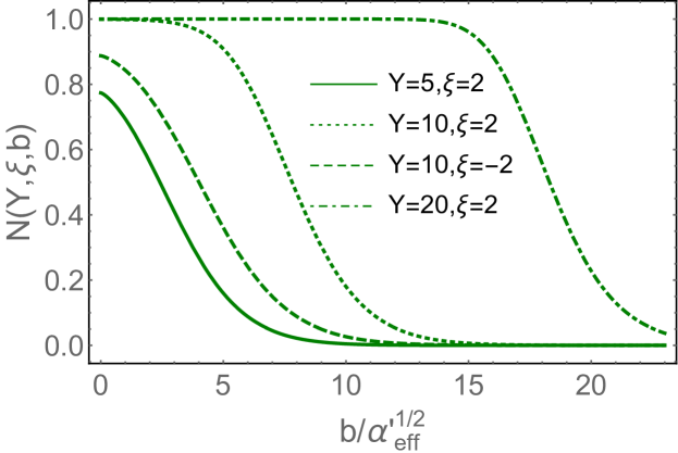
Figure 8: The impact parameter($b$) dependence of the scattering amplitude. For negative $\zeta$ of Eq. (124) we use the solution of Eq. (119), while for $\zeta\,>\,0$ Eq. (138) is solved with $C(Y,b)=0$ and ${\rm Const}=0$. $N_{0}$ is taken to be equal to 0.055 and $\bar{\alpha}_{S}$ = 0.25.

The new equation leads to restoration of the Froissart theorem. Indeed, going back to Eq. (6) one can see, that we can use Eq. (118) and Eq. (119) to estimate the value of $b_{0}$. Indeed, this value we can find from the following equation:

$$N\left(Y,\xi,b_{0}\right)\,\,=\,\,\underbrace{e^{\bar{\alpha}_{S}\chi\left(\gamma_{cr}\right)\,Y\,+\,\left(1-\gamma_{cr}\right)\,\xi\,-\,\frac{3}{4}\left(\frac{b_{0}^{4}}{4\,{\alpha^{\prime}}^{2}_{\rm eff}\,Y}\right)^{1/3}}}_{\mbox{in vicinity of the saturation scale}}\,\,=\,\,f_{0}$$ (143)

Assuming $Y\,\gg\,\xi$ we obtain

$$\frac{b_{0}}{\sqrt{{\alpha^{\prime}}_{\rm eff}}}\,\,=\,\,\left(\frac{4\bar{\alpha}_{S}\chi\left(\gamma_{cr}\right)}{3}\right)^{1/4}\,\,Y$$ (144)

Plugging this value for $b_{0}$ into Eq. (6) we have

$$\sigma_{tot}\,\,\leq\,\,2\,\pi\,b^{2}_{0}\,=\,2\,\pi\,{\alpha^{\prime}}_{\rm eff}\left(\frac{4\bar{\alpha}_{S}\chi\left(\gamma_{cr}\right)}{3}\right)^{1/2}\,\,Y^{2}$$ (145)

and the integral over $b>\,b_{0}$ gives a smaller contribution, which is of the order of $\sqrt{Y}$. Eq. (145) is the Froissart theorem in the specific realization for the QCD approach, based on the new non-linear evolution equation.

For applications one can use the simple analytical form of the solution to the non-linear equation, given in Ref.LEPP :

$$N\left(\zeta\right)\,\,=\,\,a\left(1-\exp\left(-N_{0}\,e^{\frac{1}{2}\,\zeta}\right)\right)\,\,+\,\,(1-a)\frac{N_{0}\,e^{\frac{1}{2}\,\zeta}}{1\,\,+\,\,N_{0}\,e^{\frac{1}{2}\,\zeta}}$$ (146)

which describe the numerical solution within the accuracy of 4% (see Fig. 9).

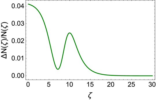
Figure 9: The comparison of the approximate analytical formula of Eq. (146) with the numerical solution of Eq. (138). $\Delta N=\left(N\left(\zeta,{Eq.~{}(\ref{BKLT7})}\right)\,.-\,N\left(\zeta,{Eq.~{}(\ref{FD6})}\right)\right)/N\left(\zeta,{Eq.~{}(\ref{BKLT7})}\right)$. Eq. (138) is solved with $C(Y,b)=0$ and ${\rm Const}=0$. $N_{0}$ is taken to be equal to 0.055 and $\bar{\alpha}_{S}$ = 0.25. In Eq. (146) $a=0.65$.

VI Conclusions

The main result of this paper is the new non-linear evolution equation which includes the random walk both in the transverse momentum and in impact parameter of the produced gluons (dipoles). We showed, that the solution to new equation results in the exponential decrease of the scattering amplitude at large impact parameter and in the restoration of the Froissart theorem. Therefore, this equation solves the long standing problem of the CGC/saturation approach. We demonstrated, that the new equation generates the amplitude, which approaches 1 for $b\,\leq\,{\rm Const}\,Y$ and which decreases as $\exp\left(-\mu b\right)$ at $b\,>\,{\rm Const}\,Y$.

We gave a brief review of the previous attempts to include the diffusion in $b$, in the framework of the BFKL equation, and showed that the new equation provides a kind of the generalization of all these attempts.

We found the solution to the equation in the kinematic region, where ${\cal Z}\,\,\ll\,\,4\,\bar{\gamma}\,Y$. Hence, a problem for the future is to develop a more general solution, as well as to describe the available experimental data within an approach, based on the new equation.

Acknowledgements.
We thank our colleagues at Tel Aviv University and UTFSM for encouraging discussions. This research was supported by CONICYT PIA/BASAL FB0821(Chile) and Fondecyt (Chile) grant 1180118 .

References

- (1) Yuri V Kovchegov and Eugene Levin, “ Quantum Choromodynamics at High Energies", Cambridge Monographs on Particle Physics, Nuclear Physics and Cosmology, Cambridge University Press, 2012 and references therein
- (2) V. S. Fadin, E. A. Kuraev and L. N. Lipatov, “On the pomeranchuk singularity in asymptotically free theories", Phys. Lett. B60, 50 (1975); E. A. Kuraev, L. N. Lipatov and V. S. Fadin, “The Pomeranchuk Singularity in Nonabelian Gauge Theories" Sov. Phys. JETP 45, 199 (1977), [Zh. Eksp. Teor. Fiz.72,377(1977)]; “The Pomeranchuk Singularity in Quantum Chromodynamics,” I. I. Balitsky and L. N. Lipatov, Sov. J. Nucl. Phys. 28, 822 (1978), [Yad. Fiz.28,1597(1978)].
- (3) L. N. Lipatov, “The Bare Pomeron in Quantum Chromodynamics,” Sov. Phys. JETP 63, 904 (1986) [Zh. Eksp. Teor. Fiz. 90, 1536 (1986)].
-
(4)
M. Froissart,
Phys. Rev. 123 (1961) 1053;
A. Martin, “Scattering Theory: Unitarity, Analitysity and Crossing." Lecture Notes in Physics, Springer-Verlag, Berlin-Heidelberg-New-York, 1969. - (5) E. M. Levin and M. G. Ryskin, “High-energy hadron collisions in QCD,” Phys. Rept. 189 (1990) 267.
- (6) E. M. Levin and M. G. Ryskin, “The Shrinkage Of The Diffraction Peak Of The Bare Pomeron In QCD,” Sov. J. Nucl. Phys. 50 (1989) 881 [Z. Phys. C 48 (1990) 231] [Yad. Fiz. 50 (1989) 1417].
- (7) E. Levin and C. I. Tan, “Heterotic pomeron: A Unified treatment of high-energy hadronic collisions in QCD,” In *Santiago de Compostela 1992, Proceedings, Multiparticle dynamics* 568-575 and Fermilab Batavia - FERMILAB-Conf-92-391 (92/09,rec.Jan.93) 9 p. (303600) Brown Univ. Providence - BROWN-HET-889 (92/09,rec.Jan.93); [hep-ph/9302308].
- (8) D. Y. Ivanov, R. Kirschner, E. M. Levin, L. N. Lipatov, L. Szymanowski and M. Wusthoff, “The BFKL pomeron in (2+1)-dimensional QCD,” Phys. Rev. D 58 (1998) 074010 doi:10.1103/PhysRevD.58.074010 [hep-ph/9804443].
- (9) D. Kharzeev and E. Levin, “Scale anomaly and ’soft’ pomeron in QCD,” Nucl. Phys. B 578 (2000) 351 doi:10.1016/S0550-3213(00)00158-9 [hep-ph/9912216].
- (10) D. E. Kharzeev, Y. V. Kovchegov and E. Levin, “QCD instantons and the soft pomeron,” Nucl. Phys. A 690 (2001) 621 doi:10.1016/S0375-9474(01)00352-9 [hep-ph/0007182].
- (11) A. Kovner and U. A. Wiedemann, “Nonlinear QCD evolution: Saturation without unitarization,” Phys. Rev. D 66, 051502 (2002) [hep-ph/0112140]; “Perturbative saturation and the soft pomeron,” Phys. Rev. D 66, 034031 (2002) [hep-ph/0204277]; ,̇ “No Froissart bound from gluon saturation,” Phys. Lett. B 551, 311 (2003) [hep-ph/0207335].
- (12) E. Ferreiro, E. Iancu, K. Itakura and L. McLerran, “Froissart bound from gluon saturation,” Nucl. Phys. A 710, 373 (2002) [hep-ph/0206241].
- (13) K. J. Golec-Biernat and A. M. Stasto, “On solutions of the Balitsky-Kovchegov equation with impact parameter,” Nucl. Phys. B 668, 345 (2003) [hep-ph/0306279].
- (14) S. Bondarenko, E. Levin and C. I. Tan, “High energy amplitude as an admixture of ’soft’ and ’hard’ pomerons,” Nucl. Phys. A 732 (2004) 73 doi:10.1016/j.nuclphysa.2003.11.056 [hep-ph/0306231].
- (15) E. Gotsman, M. Kozlov, E. Levin, U. Maor and E. Naftali, “Towards a new global QCD analysis: Solution to the nonlinear equation at arbitrary impact parameter,” Nucl. Phys. A 742, 55 (2004) [hep-ph/0401021].
- (16) Y. Hatta and A. H. Mueller, “Correlation of small-x gluons in impact parameter space,” Nucl. Phys. A 789, 285 (2007) [hep-ph/0702023 [HEP-PH]].
- (17) A. H. Mueller and S. Munier, “Correlations in impact-parameter space in a hierarchical saturation model for QCD at high energy,” Phys. Rev. D 81, 105014 (2010) [arXiv:1002.4575 [hep-ph]].
- (18) J. Berger and A. M. Stasto, “Small x nonlinear evolution with impact parameter and the structure function data,” Phys. Rev. D 84, 094022 (2011) [arXiv:1106.5740 [hep-ph]].
- (19) J. Berger and A. Stasto, “Numerical solution of the nonlinear evolution equation at small x with impact parameter and beyond the LL approximation,” Phys. Rev. D 83, 034015 (2011) [arXiv:1010.0671 [hep-ph]].
- (20) A. Kormilitzin and E. Levin, “Non-linear equation: Energy conservation and impact parameter dependence,” Nucl. Phys. A 849, 98 (2011) [arXiv:1009.1468 [hep-ph]].
- (21) E. Levin and S. Tapia, “BFKL Pomeron: modeling confinement,” JHEP 1307 (2013) 183 [arXiv:1304.8022 [hep-ph]].
- (22) E. Levin, L. Lipatov and M. Siddikov, “BFKL Pomeron with massive gluons,” Phys. Rev. D 89 (2014) 074002 [arXiv:1401.4671 [hep-ph]].
- (23) E. Levin, “Large behaviour in the CGC/saturation approach: BFKL equation with pion loops,” Phys. Rev. D 91 (2015) no.5, 054007 [arXiv:1412.0893 [hep-ph]].
- (24) O. V. Kancheli, “On the parton picture of Froissart asymptotic behavior,” arXiv:1609.07657 [hep-ph].
- (25) J. Cepila, J. G. Contreras and M. Matas, “Collinearly improved kernel suppresses Coulomb tails in the impact-parameter dependent Balitsky-Kovchegov evolution,” Phys. Rev. D 99 (2019) no.5, 051502, [arXiv:1812.02548 [hep-ph]].
- (26) D. Bendova, J. Cepila, J. G. Contreras and M. Matas, “Solution to the Balitsky-Kovchegov equation with the collinearly improved kernel including impact-parameter dependence,” Phys. Rev. D 100 (2019) no.5, 054015, [arXiv:1907.12123 [hep-ph]].
- (27) C. Contreras, E. Levin and R. Meneses, “BFKL equation in the next-to-leading order: solution at large impact parameters,” Eur. Phys. J. C 79 (2019) no.10, 842, [arXiv:1906.09603 [hep-ph]].
- (28) P. D. B. Collins, “An Introduction to Regge Theory and High-Energy Physics”, Cambridge Monographs on Mathematical Physics, Cambridge University Press ( 2009) 460 p.
- (29) Luca Caneschi (editor), “Regge Theory of Low Hadronic Interaction", North-Holland 1989.
- (30) V. N. Gribov, “ Strong Interactions of Hadrons at High Energies". Cambridge, UK: Cambridge University Press, 2008. “The theory of complex angular momenta: Gribov lectures on theoretical physics,” Cambridge Monographs on Mathematical Physics Cambridge University Press (2003) 312 p; V. N. Gribov, “Space-time description of hadron interactions at high-energies,” hep-ph/0006158; “Inelastic processes at super high-energies and the problem of nuclear cross-sections,” Sov. J. Nucl. Phys. 9, 369 (1969) [Yad. Fiz. 9, 640 (1969)].
- (31) E. Levin, “Everything about Reggeons. Part 1: Reggeons in ’soft’ interaction,” hep-ph/9710546.
- (32) R. P. Feynman, “Very high-energy collisions of hadrons,” Phys. Rev. Lett. 23, 1415 (1969). doi:10.1103/PhysRevLett.23.1415; “Photon-hadron interactions,” Reading 1972.
- (33) F. E. Low, “A Model of the Bare Pomeron,” Phys. Rev. D 12, 163 (1975). doi:10.1103/PhysRevD.12.163; S. Nussinov, “Colored Quark Version of Some Hadronic Puzzles,” Phys. Rev. Lett. 34, 1286 (1975). doi:10.1103/PhysRevLett.34.1286
- (34) A. H. Mueller, “O(2,1) analyses of single particvle spectra at high energy,” Phys. Rev. D2 (1970) 2963.
- (35) L. V. Gribov, E. M. Levin and M. G. Ryskin, “Semihard processes in QCD", Phys. Rep. 100 (1983) 1.
- (36) A. H. Mueller and J. Qiu, “Gluon recombination and shadowing at small values of ", Nucl. Phys. B268 (1986) 427
- (37) L. McLerran and R. Venugopalan, “Computing quark and gluon distribution functions for very large nuclei", Phys. Rev. D49 (1994) 2233, “Gluon distribution functions for very large nuclei at small transverse momentum", Phys. Rev. D49 (1994), 3352; ‘Green?s function in the color field of a large nucleus", D50 (1994) 2225; “ Fock space distributions, structure functions, higher twists, and small " , D59 (1999) 09400.
- (38) A. H. Mueller, “Soft Gluons In The Infinite Momentum Wave Function And The BFKL Pomeron,” Nucl. Phys. B 415, 373 (1994); “Unitarity and the BFKL pomeron,” Nucl. Phys. B 437 (1995) 107 [arXiv:hep-ph/9408245].
- (39) I. Balitsky, “Operator expansion for high-energy scattering", [arXiv:hep-ph/9509348]; “Factorization and high-energy effective action", Phys. Rev. D60, 014020 (1999) [arXiv:hep-ph/9812311]; Y. V. Kovchegov, “ Small-x structure function of a nucleus including multiple Pomeron exchanges"’ Phys. Rev. D60, 034008 (1999), [arXiv:hep-ph/9901281].
- (40) A. A. Anselm and V. N. Gribov, “Zero pion mass limit in interactions at very high-energies,” Phys. Lett. B 40, 487 (1972).
- (41) I. Gradstein and I. Ryzhik, Table of Integrals, Series, and Products, Fifth Edition, Academic Press, London, 1994.
- (42) S. R. Amendolia et al. [NA7 Collaboration], “A Measurement of the Space - Like Pion Electromagnetic Form-Factor,” Nucl. Phys. B 277, 168 (1986).
- (43) H. B. Meyer, “Glueball regge trajectories,” hep-lat/0508002.
- (44) E. Gotsman, E. Levin and I. Potashnikova, “CGC/saturation approach: secondary Reggeons and dependence on energy,” Phys. Lett. B 786 (2018) 472 doi:10.1016/j.physletb.2018.10.017 [arXiv:1807.06459 [hep-ph]]; “CGC/saturation approach: soft interaction at the LHC energies,” Phys. Lett. B 781 (2018) 155 doi:10.1016/j.physletb.2018.03.069 [arXiv:1712.06992 [hep-ph]]; “A CGC/saturation approach for angular correlations in proton-proton scattering,” Eur. Phys. J. C 77 (2017) no.9, 632 doi:10.1140/epjc/s10052-017-5204-z [arXiv:1706.07617 [hep-ph]].
- (45) A. H. Mueller and D. N. Triantafyllopoulos, “The Energy dependence of the saturation momentum,” Nucl. Phys. B 640 (2002) 331 [hep-ph/0205167];
- (46) J. Bartels and E. Levin, “Solutions to the Gribov-Levin-Ryskin equation in the nonperturbative region,” Nucl. Phys. B 387 (1992) 617. doi:10.1016/0550-3213(92)90209-T
- (47) E. Levin and K. Tuchin, “Solution to the evolution equation for high parton density QCD,” Nucl. Phys. B 573 (2000) 833, [hep-ph/9908317].
- (48) A. M. Stasto, K. J. Golec-Biernat and J. Kwiecinski, “Geometric scaling for the total gamma* p cross-section in the low x region,” Phys. Rev. Lett. 86 (2001) 596 [arXiv:hep-ph/0007192].
- (49) E. Iancu, K. Itakura and L. McLerran, “Geometric scaling above the saturation scale,” Nucl. Phys. A 708 (2002) 327 [arXiv:hep-ph/0203137].
- (50) V. N. Gribov and L. N. Lipatov, “Deep inelastic e p scattering in perturbation theory,” Sov. J. Nucl. Phys. 15, 438 (1972), [Yad. Fiz.15,781(1972)]; G. Altarelli and G. Parisi, “Asymptotic Freedom in Parton Language,” Nucl. Phys. B 126 (1977) 298. doi:10.1016/0550-3213(77)90384-4 Y. L. Dokshitzer, “Calculation of the Structure Functions for Deep Inelastic Scattering and e+ e- Annihilation by Perturbation Theory in Quantum Chromodynamics.,” Sov. Phys. JETP 46, 641 (1977), [Zh. Eksp. Teor. Fiz.73,1216(1977)].
- (51) A.D. Polyanin, .Handbook of linear partial differential equations for engineers and scientists , Chapman Hall/CRC, 2001.
- (52) A. H. Rezaeian and I. Schmidt, “Impact-parameter dependent Color Glass Condensate dipole model and new combined HERA data,” Phys. Rev. D 88 (2013) 074016, [arXiv:1307.0825 [hep-ph]].
- (53) C. Contreras, E. Levin and I. Potashnikova, “CGC/saturation approach: a new impact-parameter dependent model,” Nucl. Phys. A 948 (2016) 1 doi:10.1016/j.nuclphysa.2016.01.020 [arXiv:1508.02544 [hep-ph]].
- (54) E. Levin, “Dipole-dipole scattering in CGC/saturation approach at high energy: summing Pomeron loops,” JHEP 1311 (2013) 039 doi:10.1007/JHEP11(2013)039 [arXiv:1308.5052 [hep-ph]].