Rare event simulation for
non-Markovian repairable fault trees

Abstract

Dynamic fault trees (dft) are widely adopted in industry to assess the dependability of safety-critical equipment. Since many systems are too large to be studied numerically, dfts dependability is often analysed using Monte Carlo simulation. A bottleneck here is that many simulation samples are required in the case of rare events, e.g. in highly reliable systems where components fail seldomly. Rare event simulation (res) provides techniques to reduce the number of samples in the case of rare events. We present a res technique based on importance splitting, to study failures in highly reliable dfts. Whereas res usually requires meta-information from an expert, our method is fully automatic: By cleverly exploiting the fault tree structure we extract the so-called importance function. We handle dfts with Markovian and non-Markovian failure and repair distributions—for which no numerical methods exist—and show the efficiency of our approach on several case studies.

1 Introduction

Reliability engineering is an important field that provides methods and tools to assess and mitigate the risks related to complex systems. Fault tree analysis (fta) is a prominent technique here. Its application encompasses a large number of industrial domains that range from automotive and aerospace system engineering, to energy and telecommunication systems and protocols.

Fault trees.

A fault tree (ft) describes how component failures occur and propagate through the system, eventually leading to system failures. Technically, an ft is a directed acyclic graph whose leaves model component failures, and whose other nodes (called gates) model failure propagation. Using fault trees one can compute dependability metrics to quantify how a system fares w.r.t. certain performance indicators. Two common metrics are system reliability—the probability that there are no system failures during a given mission time—and system availability—the average percentage of time that a system is operational.

Static fault trees (aka standard fts) contain a few basic gates, like $\mathsf{{AND}}$ and $\mathsf{{OR}}$ gates. This makes them easy to design and analyse, but also limits their expressivity. Dynamic fault trees (dfts [21, 52]) are a common and widely applied extension of standard fts, catering for more complex dependability patterns, like spare management and causal dependencies. To model these patterns, dfts come with additional gates, for instance $\mathsf{{SPARE}}$, $\mathsf{{PAND}}$, and $\mathsf{{FDEP}}$.

Such gates make dfts more difficult to analyse. In static fts it only matters whether or not a component has failed, so they can be analysed with Boolean methods, such as binary decision diagrams [32]. Dynamic fault trees, on the other hand, crucially depend on the failure order, so Boolean methods are insufficient. Moreover and on top of these two classes, repairable fault trees (rft [7]) permit components to be repaired after they have failed. This is crucial to model fault-tolerant systems more realistically. Yet repairs make analyses even harder: it does not suffice to know which components failed, or in which order, but also if they are simultaneously failed. The general rule is that the more complex the formalism, the more realistic the model, and the harder the analyses.

Fig. 2 is an rft with a top $\mathsf{{AND}}$ gate, a $\mathsf{{SPARE}}$ ($\mathsf{Rcab}$), and three leaves.

Fault tree analysis.

The reliability/availability of a fault tree can be computed via numerical methods, such as probabilistic model checking. This involves exhaustive explorations of state-based models such as interactive Markov chains [48]. Since the number of states (i.e. system configurations) is exponential in the number of tree elements, analysing large trees remains a challenge today [32, 1]. Moreover, numerical methods are usually restricted to exponential failure rates and combinations thereof, like Erlang and acyclic phase type distributions [48].

Alternatively, fault trees can be analysed using (standard) Monte Carlo simulation (smc [26, 48, 45], aka statistical model checking). Here, a large number of simulated system runs (samples) is produced. Reliability and availability are then statistically estimated from the resulting sample set. Such sampling does not involve storing the full state space. Therefore, smc is much more memory efficient than numerical techniques. Furhermore, smc is not restricted to exponential probability distributions. However, a known bottleneck of smc are rare events: when the event of interest has a low probability (which is typically the case in highly reliable systems), millions of samples may be required to observe it. Producing these samples can take a unacceptably long simulation time.

Rare event simulation.

To alleviate this problem, the field of rare event simulation (res) provides techniques that reduce the number of samples [42]. The two leading techniques are importance sampling and importance splitting.

Importance sampling tweaks the probabilities in a model, then computes the metric of interest for the changed system, and finally adjusts the analysis results to the original model [28, 39]. As a simple example consider a coin whose probability of heads is $p=\nicefrac{{1}}{{80}}$. We can increase that probability to $p^{\prime}=\nicefrac{{1}}{{8}}$, but count each occurrence of heads as $\nicefrac{{1}}{{10}}$ rather than as 1. This is typically denoted change of measure. Thus, if we draw $n=1000$ samples with the increased probability $p^{\prime}$, and we see 67 heads coming up, we estimate the probability on heads as $0.067=\frac{67}{1000}\cdot\frac{1}{10}$. In the limit $n\rightarrow\infty$, the expected number of heads that come up is the same for the original and the tweaked model (after the adjustment). However, sample outcomes have a lower variance in the tweaked model, so statistical analyses converge faster: few samples yield accurate estimations.

Importance splitting, deployed in this paper, relies on rare events that arise as a sequential combination of less rare intermediate events [34, 3]. We exploit this fact by generating more (partial) samples on paths where such intermediate events are observed. In the coin example, suppose we flip it eight times in a row, and say we are interested in observing at least three heads. If heads comes up at the first flip ($H$) then we are on a promising path. We can then clone (split) the current path $H$, generating e.g. 7 copies of it, each copy evolving independently from the second flip onwards. Say one of them observes three heads—the cloned $H$ plus two more. Then each observation of the rare event (three heads) is counted as $\nicefrac{{1}}{{7}}$ rather than as 1, to account for the splitting that spawned the clone. Now, if a clone observes a new head ($HH$), this is even more promising than $H$, so the splitting mechanism can be repeated. If we make 5 copies of the $HH$ clone, then observing the event of interest in any of these copies counts as $\frac{1}{35}=\frac{1}{7}\cdot\frac{1}{5}$. Alternatively, observing tails as second flip ($HT$) is less promising than heads. One could then decide not to split such path.

This example highlights a key ingredient of importance splitting: the importance function, that indicates for each state how promising it is w.r.t. the event of interest. This function, together with other parameters such as thresholds [23], are used to choose e.g. the number of clones spawned when visiting a state. An importance function for our example could be the number of heads seen thus far. Another one could be such number, multiplied by the number of coin flips yet to come. The goal is to give higher importance to states from which observing the rare event is more likely. The efficiency of an importance splitting implementation increases as the importance function better reflects such property.

Rare event simulation has been successfully applied in several domains [41, 54, 58, 5, 6, 55]. However, a key bottleneck is that it critically relies on expert knowledge. In particular for importance splitting, finding a good importance function is a well-known highly non-trivial task [42, 31].

Our contribution: rare event simulation for fault trees.

This paper presents an importance splitting method to analyse rfts. In particular, we automatically derive an importance function by exploiting the description of a system as a fault tree. This is crucial, since the importance function is normally given manually in an ad hoc fashion by a domain or res expert. We use a variety of res algorithms based in our importance function, to estimate system unreliability and unavailability. Our approach can converge to precise estimations in increasingly reliable systems. This method has four advantages over earlier analysis methods for rfts—which we overview in the related work section 7—namely: (1) we are able to estimate both the system reliability and availability; (2) we can handle arbitrary failure and repair distributions; (3) we can handle rare events; and (4) we can do it in a fully automatic fashion.

Technically, we build local importance functions for the (automata-semantics of the) nodes of the tree. We then aggregate these local functions into an importance function for the full tree. Aggregation uses structural induction in the layered description of the tree. Using our importance function, we implement importance splitting methods to run res analyses. We implemented our theory in a full-stack tool chain. With it, we computed confidence intervals for the unreliability and unavailability of several case studies. Our case studies are rfts whose failure and repair times are governed by arbitrary continuous probability density functions (pdfs). Each case study was analysed for a fixed runtime budget and in increasingly resilient configurations. In all cases our approach could estimate the narrowest intervals for the most resilient configurations.

Organization of the paper.

We first introduce the formal concepts used for our mathematical definitions in Secs. 2 and 3. Then, we detail our theory to implement res for repairable dfts with arbitrary pdfs in Sec. 4. For that, Sec. 4.1 introduces our (compositional) importance function, and Sec. 4.2 explains how to embed it into an automated framework for Importance Splitting res. Next, Sec. 5 describes how we implement this theory in our tool chain. In Sec. 6 we show an extensive experimental evaluation that corroborates our expectations. We finally overview related work in Sec. 7, and conclude our contributions in Sec. 8.

Scope	Abbreviation	Meaning
General	pdf	Probability density function
	ci	Confidence interval
	fta	Fault Tree Analysis
	ft	Fault Tree
	dft	Dynamic Fault Tree
	rft	Repairable (Dynamic) Fault Tree
	smc	Standard Monte Carlo simulation
	res	Rare Event Simulation
	iosa	Input/Output Stochastic Automata with Urgency [19]
Tree gates ($m$ inputs)	$\mathsf{{AND}}$	Conjunction: $m$-ary AND
	$\mathsf{{OR}}$	Disjunction: $m$-ary OR
	$\mathsf{{VOT}}_{k}$	Voting: $k$ out of $m$
	$\mathsf{{PAND}}$	Priority AND
	$\mathsf{{SPARE}}$	Spare: 1 primary $\mathsf{{BE}}$, $m$-$1$ spare $\mathsf{{BE}}$s
	$\mathsf{{FDEP}}$	Functional dependency: 1 trigger, $m$-$1$ dependent $\mathsf{{BE}}$s
Other tree nodes	$\mathsf{{BE}}$	Basic element
	$\mathsf{{SBE}}$	Spare basic element
	$\mathsf{{RBOX}}$	Repair box
Case studies	VOT	Voting gates (synthetic)
	DSPARE	Double-spare gates (synthetic)
	RWC	Railway cabinets [25, 46]
	HVC	High voltage cab. (RWC subsys.)
	RC	Relay cab. (RWC subsys.)
	FTPP	Fault tolerant parallel processor [21]
	HECS	Hypothetical example computer system [52]

Table 1: Glossary of acronyms and abbreviations

2 Fault tree analysis

A fault tree ‘$\triangle$’ is a directed acyclic graph that models how component failures propagate and eventually cause the full system to fail. We consider repairable fault trees (RFTs), where failures and repairs are governed by arbitrary probability distributions.

(a) ​$\mathsf{{AND}}$

(b) ​$\mathsf{{OR}}$

(c) ​$\mathsf{{VOT}}_{k}$

(d) ​$\mathsf{{PAND}}$

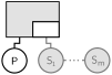
(e) ​$\mathsf{{SPARE}}$

(f) ​$\mathsf{{FDEP}}$

(g) $\mathsf{{RBOX}}$

Figure 1: Fault tree gates and the repair box

Basic elements.

The leaves of the tree, called basic events or basic elements ($\mathsf{{BE}}$s), model the failure of components. A $\mathsf{{BE}}$ $b$ is equipped with a failure distribution $F_{b}$ that governs the probability for $b$ to fail before time $t$, and a repair distribution $R_{b}$ governing its repair time. Some $\mathsf{{BE}}$s are used as spare components: these ($\mathsf{{SBE}}$s) replace a primary component when it fails. $\mathsf{{SBE}}$s are equipped also with a dormancy distribution $D_{b}$, since spares fail less often when dormant, i.e. not in use. Only if an $\mathsf{{SBE}}$ becomes active, its failure distribution is given by $F_{b}$.

Gates.

Non-leave nodes are called intermediate events and are labelled with gates, describing how combinations of lower failures propagate to upper levels. Fig. 1 shows their syntax. Their meaning is as follows: the $\mathsf{{AND}}$, $\mathsf{{OR}}$, and $\mathsf{{VOT}}_{k}$ gates fail if respectively all, one, or $k$ of their $m$ children fail (with $1\leqslant k\leqslant m$). The latter is called the voting or $k$ out of $m$ gate. Note that $\mathsf{{VOT}}_{1}$ is equivalent to an $\mathsf{{OR}}$ gate, and $\mathsf{{VOT}}_{m}$ is equivalent to an $\mathsf{{AND}}$. The priority-and gate ($\mathsf{{PAND}}$) is an $\mathsf{{AND}}$ gate that only fails if its children fail from left to right (or simultaneously). $\mathsf{{PAND}}$s express failures that can only happen in a particular order, e.g. a short circuit in a pump can only occur after a leakage. $\mathsf{{SPARE}}$ gates have one primary child and one or more spare children: spares replace the primary when it fails. The $\mathsf{{FDEP}}$ gate has an input trigger and several dependent events: all dependent events become unavailable when the trigger fails. $\mathsf{{FDEP}}$s can model for instance networks elements that become unavailable if their connecting bus fails.

Repair boxes.

An $\mathsf{{RBOX}}$ determines which basic element is repaired next according to a given policy. Thus all its inputs are $\mathsf{{BE}}$s or $\mathsf{{SBE}}$s. Repair events of basic elements propagate along the tree analogously to fail events. Unlike gates, an $\mathsf{{RBOX}}$ has no output since it does not propagate failures.

Top level event.

A full-system failure occurs if the top event (i.e. the root node) of the tree fails.

Example.

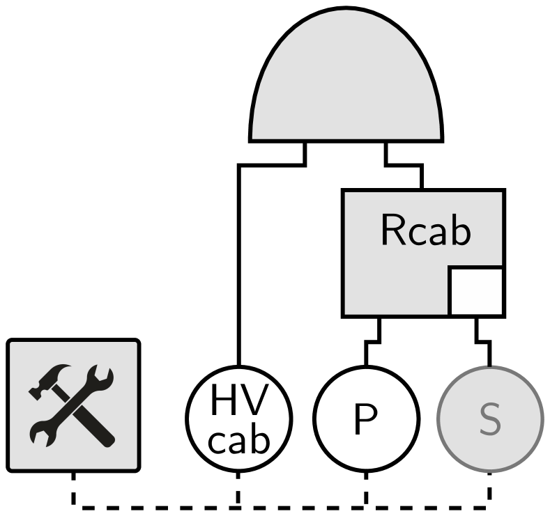
Figure 2: ​Tiny rft ​​

The tree in Fig. 2 models a railway-signal system, which fails if its high voltage and relay cabinets fail [25, 46]. Thus, the top event is an $\mathsf{{AND}}$ gate with children $\mathsf{HVcab}$ (a $\mathsf{{BE}}$) and $\mathsf{Rcab}$. The latter is a $\mathsf{{SPARE}}$ gate with primary $\mathsf{P}$ and spare $\mathsf{S}$. All $\mathsf{{BE}}$s are managed by one $\mathsf{{RBOX}}$ with repair priority $\mathsf{HVcab}>\mathsf{P}>\mathsf{S}$.

Notation.

The nodes of a tree $\triangle$ are given by $\mathit{nodes}(\triangle)=\{0,1,\ldots,n-1\}$. We let $v,w$ range over $\mathit{nodes}(\triangle)$. A function $\mathit{type}^{\triangle}\colon\mathit{nodes}(\triangle)\to\{\mathsf{{BE}},\mathsf{{SBE}},\mathsf{{AND}},\mathsf{{OR}},\allowbreak\mathsf{{VOT}}_{k},\mathsf{{PAND}},\mathsf{{SPARE}},\mathsf{{FDEP}},\allowbreak\mathsf{{RBOX}}\}$ yields the type of each node in the tree. A function $\mathit{chil}^{\triangle}\colon\mathit{nodes}(\triangle)\to\mathit{nodes}(\triangle)^{*}$ returns the ordered list of children of a node. If clear from context, we omit the superscript $\triangle$ from function names.

Semantics.

The semantics of static fault trees, i.e. trees that only feature the static gates $\mathsf{{AND}}$, $\mathsf{{OR}}$ and $\mathsf{{VOT}}_{k}$, can be given as a Boolean function. For the gates $\mathsf{{PAND}},\mathsf{{SPARE}},\mathsf{{FDEP}}$ the order of the failures matter, so a Boolean function does not suffice. Therefore, the semantics for (repairable) dynamic fault trees is given in terms of stochastic transition models, such as Markov automata, Petri nets, iosa, etc. Following [38] we give semantics to rft as Input/Output Stochastic Automata (iosa), so that we can handle arbitrary probability distributions. Each state in the iosa represents a system configuration, indicating which components are operational and which have failed. Transitions among states describe how the configuration changes when failures or repairs occur.

More precisely, a state in the iosa is a tuple $\boldsymbol{x}=(\boldsymbol{x}_{0},\ldots,\boldsymbol{x}_{n-1})\in\pazocal{S}\subseteq\mathbb{N}^{n}$, where $\pazocal{S}$ is the state space and $\boldsymbol{x}_{v}$ denotes the state of node $v$ in $\triangle$. The possible values for $\boldsymbol{x}_{v}$ depend on the type of $v$. The output $\boldsymbol{z}_{v}\in\{0,1\}$ of node $v$ indicates whether it is operational ($\boldsymbol{z}_{v}{=}0$) or failed ($\boldsymbol{z}_{v}{=}1$) and is calculated as follows:

• $\mathsf{{BE}}$s (white circles in Fig. 1) have a binary state: $\boldsymbol{x}_{v}=0$ if $\mathsf{{BE}}$ $v$ is operational and $\boldsymbol{x}_{v}=1$ if it is failed. The output of a $\mathsf{{BE}}$ is its state: $\boldsymbol{z}_{v}=\boldsymbol{x}_{v}$.

• $\mathsf{{SBE}}$s (gray circles in Fig. 1(e)) have two additional states: $\boldsymbol{x}_{v}=2,3$ if a dormant $\mathsf{{SBE}}$ $v$ is resp. operational, failed. Here $\boldsymbol{z}_{v}=\boldsymbol{x}_{v}\bmod 2$.

• $\mathsf{{AND}}$s have a binary state. Since the $\mathsf{{AND}}$ gate $v$ fails iff all children fail: $\boldsymbol{x}_{v}=\min_{w\in\mathit{chil}(v)}\boldsymbol{z}_{w}$. An $\mathsf{{AND}}$ gate outputs its internal state: $\boldsymbol{z}_{v}=\boldsymbol{x}_{v}$.

• $\mathsf{{OR}}$ gates are analogous to $\mathsf{{AND}}$ gates, but fail iff any child fail, i.e. $\boldsymbol{z}_{v}=\boldsymbol{x}_{v}=\max_{w\in\mathit{chil}(v)}\boldsymbol{z}_{w}$ for $\mathsf{{OR}}$ gate $v$.

• $\mathsf{{VOT}}$ gates also have a binary state: a $\mathsf{{VOT}}_{k}$ gate fails iff $1\leqslant k\leqslant m$ children fail, thus $\boldsymbol{z}_{v}=\boldsymbol{x}_{v}=1$ if $k\leqslant\sum_{w\in\mathit{chil}(v)}\boldsymbol{z}_{w}$, and $\boldsymbol{z}_{v}=\boldsymbol{x}_{v}=0$ otherwise.

• $\mathsf{{PAND}}$ gates admit multiple states to represent the failure order of the children. For $\mathsf{{PAND}}$ $v$ with two children we let $\boldsymbol{x}_{v}$ equal: $\boldsymbol{0}$ if both children are operational; $\boldsymbol{1}$ if the left child failed, but the right one has not; $\boldsymbol{2}$ if the right child failed, but the left one has not; $\boldsymbol{3}$ if both children have failed, the right one first; $\boldsymbol{4}$ if both children have failed, otherwise. The output of $\mathsf{{PAND}}$ gate $v$ is $\boldsymbol{z}_{v}=1$ if $\boldsymbol{x}_{v}=4$ and $\boldsymbol{z}_{v}=0$ otherwise. $\mathsf{{PAND}}$ gates with more children are handled by exploiting $\mathsf{{PAND}}(w_{1},w_{2},w_{3})=\mathsf{{PAND}}(\mathsf{{PAND}}(w_{1},w_{2}),w_{3})$.

• $\mathsf{{SPARE}}$ gate $v$ leftmost input is its primary $\mathsf{{BE}}$. All other (spare) inputs are $\mathsf{{SBE}}$s. $\mathsf{{SBE}}$s can be shared among $\mathsf{{SPARE}}$ gates. When the primary of $v$ fails, it is replaced with an available $\mathsf{{SBE}}$. An $\mathsf{{SBE}}$ is unavailable if it is failed, or if it is replacing the primary $\mathsf{{BE}}$ of another $\mathsf{{SPARE}}$. The output of $v$ is $\boldsymbol{z}_{v}=1$ if its primary is failed and no spare is available. Else $\boldsymbol{z}_{v}=0$.

• An $\mathsf{{FDEP}}$ gate has no output. All inputs are $\mathsf{{BE}}$s and the leftmost is the trigger. We consider non-destructive $\mathsf{{FDEP}}$s [8]: if the trigger fails, the output of all other $\mathsf{{BE}}$ is set to $1$, without affecting the internal state. Since this can be modelled by a suitable combination of $\mathsf{{OR}}$ gates [38], we omit the details.

For example, the rft from Fig. 2 starts with all operational elements, so the initial state is $\boldsymbol{x}^{0}=(0,0,2,0,0)$. If then $\mathsf{P}$ fails, $\boldsymbol{x}_{\mathsf{P}}$ and $\boldsymbol{z}_{\mathsf{P}}$ are set to 1 (failed) and $\mathsf{S}$ becomes $\boldsymbol{x}_{\mathsf{S}}=0$ (active and operational spare), so the state changes to $\boldsymbol{x}^{1}=(0,1,0,0,0)$. The traces of the iosa are given by $\boldsymbol{x}^{0}\boldsymbol{x}^{1}\cdots\boldsymbol{x}^{n}\in\pazocal{S}^{\ast}$, where a change from $\boldsymbol{x}^{j}$ to $\boldsymbol{x}^{j+1}$ corresponds to transitions triggered in the iosa.

Nondeterminism.

Dynamic fault trees may exhibit nondeterministic behaviour as a consequence of underspecified failure behaviour [17, 33]. This can happen e.g. when two $\mathsf{{SPARE}}$s have a single shared $\mathsf{{SBE}}$: if all elements are failed, and the $\mathsf{{SBE}}$ is repaired first, the failure behaviour depends on which $\mathsf{{SPARE}}$ gets the $\mathsf{{SBE}}$. Monte Carlo simulation, however, requires fully stochastic models and cannot cope with nondeterminism. To overcome this problem we deploy the theory from [19, 38]. If a fault tree adheres to some mild syntactic conditions, then its iosa semantics is weakly deterministic, meaning that all resolutions of the nondeterministic choices lead to the same probability value. In particular, we require that (1) each $\mathsf{{BE}}$ is connected to at most one $\mathsf{{SPARE}}$ gate, and (2) $\mathsf{{BE}}$s and $\mathsf{{SBE}}$s connected to $\mathsf{{SPARE}}$s are not connected to $\mathsf{{FDEP}}$s. In addition to this, some semantic decisions have been fixed, e.g. the semantics of $\mathsf{{PAND}}$ is fully specified, and policies should be provided for $\mathsf{{RBOX}}$ and spare assignments.

Dependability metrics.

An important use of fault trees is to compute relevant dependability metrics. Let $\{X_{t}\}_{t\geqslant 0}$ be the stochastic process induced by $\triangle$ [15], and let $X_{t,v}$ be the random variable that represents the (distribution of the) state of the top event of $\triangle$ at time $t$. We focus on two popular metrics:

• system reliability: is the continuity of correct service, i.e.  the probability of observing no top event failure before some mission time $T>0$, viz. $\mathrm{REL}_{T}=\mathit{Prob}\left(\forall_{t\in[0,T]}\,.\,X_{t,v}=0\right);$

• system availability: the proportion of time that the system remains operational in the long-run, viz. $\mathrm{AVA}=\lim_{t\to\infty}\mathit{Prob}\left(X_{t,v}=0\right)$.

System unreliability and unavailability are the reverse of these metrics. That is: $\mathrm{UNREL}_{T}=1-\mathrm{REL}_{T}$ and $\mathrm{UNAVA}=1-\mathrm{AVA}$.

3 Stochastic simulation for Fault Trees

Input-Output Stochastic Automata (IOSA).

iosa [19, 18] are an extension of GSMP [49] amenable to compositional modelling. An iosa is a state-transition system where the residence time in a state is governed by a pdf. iosas feature two ingredients that are crucial for our analysis: (1) residence times can be governed by arbitrary probability distributions described by real-valued clocks, and (2) discrete transitions are labelled by actions, and allow automata to communicate with each other.

To record the passage of time and control the occurrence of events, iosa use real-valued variables called clocks. Clocks are set to a positive random value according to the (state-dependent) associated pdf. As time evolves, all clocks count down from their respective values at the same rate. When the value of a clock reaches zero it may trigger some action. Thus, to model $\mathsf{{BE}}$ $e$ in a fault tree, we associate a clock to $F_{e}$ and another to $R_{e}$. As a matter of fact, each node in an ft is modelled as an iosa automaton. The propagation of fail/repair events in the tree is done by (discrete, instantaneous) action synchronisation among automata. Formally:

Definition 1 (iosa [19]).

An Input/Output Stochastic Automaton with Urgency is a tuple $\left(\pazocal{S},\pazocal{A},\pazocal{C},\xrightarrow{{}},s_{0},C_{0}\right)$ where: (i) $\pazocal{S}$is a denumerable set of states; (ii) $\pazocal{A}$is a denumerable set of labels partitioned into input labels $\pazocal{A}^{\mathsf{i}}$ and output labels $\pazocal{A}^{\mathsf{o}}$, where $\pazocal{A}^{\mathsf{u}}\subseteq\pazocal{A}$ are urgent labels; (iii) $\pazocal{C}$is a finite set of clocks s.t. each $x\in\pazocal{C}$ has an associated continuous probability measure $\mu_{x}$ with support on $\mathbb{R}_{>0}$; (iv) ${\xrightarrow{{}}}\subseteq\pazocal{S}\times\pazocal{C}\times\pazocal{A}\times\pazocal{C}\times\pazocal{S}$is a transition function; (v) $s_{0}\in\pazocal{S}$is the initial state; and (vi) $C_{0}\subseteq\pazocal{C}$are clocks initialized in $s_{0}$.

Six constraints on $\xrightarrow{{}}$ ensure that, in closed iosa obtained from the parallel composition of all automata, nondeterminism is restricted to urgent actions. These semantic constraints are translated into the syntactic conditions previously mentioned for fts. For insights see [19]; details on how to represent gates and basic elements with iosa automata are in [38].

Modelling fault trees as iosa allows us to perform Monte Carlo simulation: we generate traces, i.e. sequences of states $\boldsymbol{x}^{0},\boldsymbol{x}^{1},\ldots,\boldsymbol{x}^{m}$ where each $\boldsymbol{x}^{j},\boldsymbol{x}^{j+1}$ is the projection on $\pazocal{S}^{2}$ of an element of $\xrightarrow{{}}$ from Def. 1. Then, we estimate dependability metrics via statistical analyses on a set of sampled traces.

Standard Monte Carlo simulation (SMC).

Monte Carlo simulation takes random samples from stochastic models to estimate a (dependability) metric of interest. For instance, to estimate the unreliability of a tree $\triangle$ we sample $N$ independent traces from its iosa semantics. An unbiased statistical estimator for $p=\mathrm{UNREL}_{T}$ is the proportion of traces observing a top level event, that is, $\hat{p}_{N}=\frac{1}{N}\sum_{j=1}^{N}X^{j}$ where $X^{j}=1$ if the $j$-th trace exhibits a top level failure before time $T$ and $X^{j}=0$ otherwise. The statistical error of $\hat{p}$ is typically quantified with two numbers $\delta$ and $\varepsilon$ s.t. $\hat{p}\in[p-\varepsilon,p+\varepsilon]$ with probability $\delta$. The interval $\hat{p}\pm\varepsilon$ is called a confidence interval (ci) with coefficient $\delta$ and precision $2\varepsilon$.

Such procedures scale linearly with the number of tree nodes and cater for a wide range of pdfs, even non-Markovian distributions. However, they encounter a bottleneck to estimate rare events: if $p\approx 0$, very few traces observe $X^{j}=1$. Therefore, the variance of estimators like $\hat{p}$ becomes huge, and cis become very broad, easily degenerating to the trivial interval $[0,1]$. Increasing the number of traces alleviates this problem, but even standard ci settings—where $\varepsilon$ is relative to $p$—require sampling an unacceptable number of traces [42]. For instance, choosing $\delta=0.95$ and $\varepsilon=\frac{p}{10}$ (“95% confidence and 10% relative error”) requires $N\geqslant\nicefrac{{384}}{{p}}$ samples. Thus if $\mathrm{UNREL}_{T}\approx 10^{-8}$, one needs $N\geqslant 38400000000$ traces, making the simulation times unacceptably long. Rare event simulation techniques solve this specific problem.

Rare Event Simulation (RES).

res techniques [42] increase the amount of traces that observe the rare event, e.g. a top level event in an rft. Two prominent classes of res techniques are importance sampling, which adjusts the pdf of failures and repairs, and importance splitting (isplit [36]), which samples more (partial) traces from states that are closer to the rare event. We focus on isplit due to its flexibility with respect to the probability distributions.

isplit can be efficiently deployed as long as the rare event $\gamma$ can be described as a nested sequence of less-rare events $\gamma=\gamma_{M}\subsetneq\gamma_{M-1}\subsetneq\cdots\subsetneq\gamma_{0}$. This decomposition allows isplit to study the conditional probabilities $p_{k}=\mathit{Prob}(\gamma_{k+1}\,|\,\gamma_{k})$ separately, to then compute $p=\mathit{Prob}(\gamma)=\prod_{k=0}^{M\text{-}1}\mathit{Prob}(\gamma_{k+1}\,|\,\gamma_{k})$. Moreover, isplit requires all conditional probabilities $p_{k}$ to be much greater than $p$, so that estimating each $p_{k}$ can be done efficiently with smc.

The key idea behind isplit is to define the events $\gamma_{k}$ via a so called importance function $\pazocal{I}\colon\pazocal{S}\to\mathbb{N}$ that assigns an importance to each state $s\in\pazocal{S}$. The higher the importance of a state, the closer it is to the rare event $\gamma_{M}$. Event $\gamma_{k}$ collects all states with importance at least $\ell_{k}$, for certain sequence of threshold levels $0=\ell_{0}<\ell_{1}<\cdots<\ell_{M}$. Formally: $\gamma_{k}=\{s\in\pazocal{S}\mid\pazocal{I}\left(s\right)\geqslant\ell_{k}\}$. In other words, a higher importance is assigned to states from which it is more likely to observe the rare event. That is, for $s,s^{\prime}\in\pazocal{S}$ s.t. $s\in\gamma_{k}$ and $s^{\prime}\in\gamma_{k^{\prime}}$, one wants $\pazocal{I}\left(s\right)<\pazocal{I}\left(s^{\prime}\right)$ iff $k<k^{\prime}$. Because then, in the nested sequence of events $\gamma_{0}\supsetneq\cdots\supsetneq\gamma_{M}$, each step $\gamma_{k-1}\boldsymbol{\rightarrow}\gamma_{k}$ makes it more likely to observe the rare event. Therefore, choosing many thresholds ($M\gg 0$) all very close to each other, one ensures that $\mathit{Prob}(\gamma_{k}\,|\,\gamma_{k-1})\gg 0$ for all $0<k\leqslant M$. Simply put, one makes a lot of baby steps in the right direction.

To exploit the importance function $\pazocal{I}$ in the simulation procedure, isplit samples more (partial) traces from states with higher importance. Two well-known methods are deployed and compared in this paper: Fixed Effort and restart. Fixed Effort (fe [23]) samples a predefined amount of traces in each region $\pazocal{S}_{k}=\gamma_{k}\setminus\gamma_{k+1}=\{s\in\pazocal{S}\mid\ell_{k+1}>\pazocal{I}(s)\geqslant\ell_{k}\}$. Thus, starting at $\gamma_{0}$ it first estimates the proportion of traces that reach $\gamma_{1}$, i.e. $p_{0}=\mathit{Prob}(\gamma_{1}\,|\,\gamma_{0})=\mathit{Prob}(\pazocal{S}_{0})$. Next, from the states that reached $\gamma_{1}$ new traces are generated to estimate $p_{1}=\mathit{Prob}(\pazocal{S}_{1})$, and so on until $p_{M}$. Fixed Effort thus requires that ($i$) each trace has a clearly defined “end,” so that estimations of each $p_{k}$ finish with probability 1, and ($ii$) all rare events reside in the uppermost region. In particular, using fe for steady-state analysis (e.g. to estimate $\mathrm{UNAVA}$) requires regeneration theory [23], which is hard to apply to non-Markovian models.

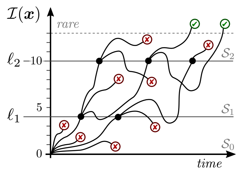
(a) fe-5 for $\mathit{Prob}(\lnot\text{\color[rgb]{0.75,0,0}\,\char 56}\,\mathsf{U}\text{\color[rgb]{0,0.55,0}\,\char 52})$

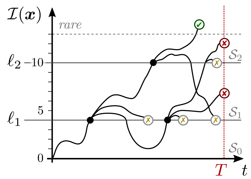
(b) rst-es for $\mathrm{UNREL}_{T}$

Figure 3: Importance Splitting algorithms Fixed Effort & restart

Example.

Fig. 3(a) shows Fixed Effort estimating the probability to visit states labelled  ✔ before others labelled  ✘. States  ✔ have importance >13, and thresholds $\ell_{1},\ell_{2}=4,10$ partition the state space in regions $\{\pazocal{S}_{i}\}_{i=0}^{2}$ s.t. all $\text{\color[rgb]{0,0.55,0}\,\char 52}\in\pazocal{S}_{2}$. The effort is 5 simulations per region, for all regions: we call this algorithm fe-5. In region $\pazocal{S}_{0}$, 2 simulations made it from the initial state to threshold $\ell_{1}$, i.e. they reached some state with importance 4 before visiting a state  ✘. In $\pazocal{S}_{1}$, starting from these two states, 3 simulations reached $\ell_{2}$. Finally, 2 out of 5 simulations visited states  ✔ in $\pazocal{S}_{2}$. Thus, the estimated rare event probability of this run of fe 5 is $\hat{p}=\prod_{i=1}^{2}\hat{p_{i}}=\frac{2}{5}\frac{3}{5}\frac{2}{5}=9.6\times 10^{-2}$.

RESTART (rst- [57, 56]) is another res algorithm, which starts one trace in $\gamma_{0}$ and monitors the importance of the states visited. If the trace up-crosses threshold $\ell_{1}$, the first state visited in $\pazocal{S}_{1}$ is saved and the trace is cloned, aka split—see Fig. 3(b). This mechanism rewards traces that get closer to the rare event. Each clone then evolves independently, and if one up-crosses threshold $\ell_{2}$ the splitting mechanism is repeated. Instead, if a state with importance below $\ell_{1}$ is visited, the trace is truncated ( in Fig. 3(b)). In general, each clone is truncated as soon as it visits a state with importance lower than its level of creation. This penalises traces that move away from the rare event. To avoid truncating all traces, the one that spawned the clones in region $\pazocal{S}_{k}$ can go below importance $\ell_{k}$. To deploy an unbiased estimator for $p$, restart measures how much split was required to visit a rare state [56]. In particular, restart does not need the rare event to be defined as $\gamma_{M}$ [53], and it was devised for steady-state analysis [57] (e.g. to estimate $\mathrm{UNAVA}$) although it can also been used for transient studies as depicted in Fig. 3(b) [54].

4 Importance Splitting for FTA

The effectiveness of isplit crucially relies on the choice of the importance function $\pazocal{I}$ as well as the threshold levels $\ell_{k}$ [36]. Traditionally, these are given by domain and/or res experts, requiring a lot of domain knowledge. This section presents a technique to obtain $\pazocal{I}$ and the $\ell_{k}$ automatically for an rft.

4.1 Compositional importance functions for Fault Trees

By the core idea behind importance splitting, states that are more likely to lead to the rare event should have a higher importance. To achieve this, the key lies in defining an importance function $\pazocal{I}$ and thresholds $\ell_{k}$ that are sensitive to both the state space $\pazocal{S}$ and the transition probabilities of the system. For us, $\pazocal{S}\subseteq\mathbb{N}^{n}$ are all possible states of a repairable fault tree (rft). Its top event fails when certain nodes fail in certain order, and remain failed before certain repairs occur. To exploit this for isplit, the structure of the tree must be embedded into $\pazocal{I}$.

The strong dependence of the importance function $\pazocal{I}$ on the structure of the tree is easy to see in the following example. Take the rft $\triangle$ from Fig. 2 and let its current state $\boldsymbol{x}$ be s.t. $\mathsf{P}$ is failed and $\mathsf{HVcab}$ and $\mathsf{S}$ are operational. If the next event is a repair of $\mathsf{P}$, then the new state $\boldsymbol{x}^{\prime}$ (where all basic elements are operational) is farther from a failure of the top event. Hence, a good importance function should satisfy $\pazocal{I}\left(\boldsymbol{x}\right)>\pazocal{I}\left(\boldsymbol{x}^{\prime}\right)$. Oppositely, if the next event had been a failure of $\mathsf{S}$ leading to state $\boldsymbol{x}^{\prime\prime}$, then one would want that $\pazocal{I}\left(\boldsymbol{x}\right)<\pazocal{I}\left(\boldsymbol{x}^{\prime\prime}\right)$. The key observation is that these inequalities depend on the structure of $\triangle$ as well as on the failures/repairs of basic elements. Because if instead of an $\mathsf{{AND}}$, the top event were a $\mathsf{{PAND}}$ gate (call this tree $\triangle^{\!\!\ast}$), the importance function should behave in the exact opposite way. That is, in tree $\triangle^{\!\!\ast}$ one wants that $\pazocal{I}\left(\boldsymbol{x}\right)>\pazocal{I}\left(\boldsymbol{x}^{\prime\prime}\right)$, since in $\boldsymbol{x}^{\prime\prime}$ the right child of the top $\mathsf{{PAND}}$ has failed before the left child. When this happens, $\mathsf{{PAND}}$ gates go into an out-of-order internal state, and cannot output a failure. So the same step from $\boldsymbol{x}$ to $\boldsymbol{x}^{\prime\prime}$ has completely different meanings for $\triangle$ and for $\triangle^{\!\!\ast}$, as a result of their structure being different.

In view of the above, any attempt to define an importance function for an arbitrary fault tree $\triangle$ must put its gate structure in the forefront. In Table 2 we introduce a compositional heuristic for this, which defines local importance functions distinguished per node type. The importance function associated to node $v$ is $\pazocal{I}_{v}\colon\mathbb{N}^{n}\to\mathbb{N}$. We define the global importance function of the tree ($\pazocal{I}_{\triangle}$ or simply $\pazocal{I}$) as the local importance function of the top event node of $\triangle$.

Table 2: Compositional importance function for rfts.

$\mathit{type}(v)$	$\pazocal{I}_{v}(\boldsymbol{x})$
$\mathsf{{BE}}$, $\mathsf{{SBE}}$	$\displaystyle\boldsymbol{z}_{v}$
$\mathsf{{AND}}$	$\mathrm{lcm}_{v}\cdot\scalebox{1.15}{$\sum_{w\in\mathit{chil}(v)}\frac{\pazocal{I}_{w}(\boldsymbol{x})}{\max^{\pazocal{I}}_{w}}$}$
$\mathsf{{OR}}$	$\displaystyle\mathrm{lcm}_{v}\cdot\max_{w\in\mathit{chil}(v)}\left\{\scalebox{1.15}{$\frac{\pazocal{I}_{w}(\boldsymbol{x})}{\max^{\pazocal{I}}_{w}}$}\right\}$
$\mathsf{{VOT}}_{k}$	$\displaystyle\mathrm{lcm}_{v}\cdot\max_{W\subseteq\mathit{chil}(v),|W|=k}\left\{\scalebox{1.15}{$\sum_{w\in W}\frac{\pazocal{I}_{w}(\boldsymbol{x})}{\max^{\pazocal{I}}_{w}}$}\right\}$
$\mathsf{{SPARE}}$	$\displaystyle\mathrm{lcm}_{v}\cdot\max\Big{(}\scalebox{1.15}{$\sum_{w\in\mathit{chil}(v)}\frac{\pazocal{I}_{w}(\boldsymbol{x})}{\max^{\pazocal{I}}_{w}}$}\leavevmode\nobreak\ ,\leavevmode\nobreak\ \boldsymbol{z}_{v}\cdot m\Big{)}$
$\mathsf{{PAND}}$	$\displaystyle\mathrm{lcm}_{v}\cdot\max\Big{(}\scalebox{1.15}{$\frac{\pazocal{I}_{l}(\boldsymbol{x})}{\max^{\pazocal{I}}_{l}}$}+\mathit{ord}\>\scalebox{1.15}{$\frac{\pazocal{I}_{r}(\boldsymbol{x})}{\max^{\pazocal{I}}_{r}}$}\leavevmode\nobreak\ ,\leavevmode\nobreak\ \boldsymbol{z}_{v}\cdot 2\Big{)}$
	where $\mathit{ord}=1$ if $\boldsymbol{x}_{v}\in\{1,4\}$ and $\mathit{ord}=-1$ otherwise
with  $\max^{\pazocal{I}}_{v}=\max_{\boldsymbol{x}\in\pazocal{S}}\pazocal{I}_{v}(\boldsymbol{x})$  and  $\mathrm{lcm}_{v}=\mathrm{lcm}\left\{\max^{\pazocal{I}}_{w}\,\middle|\,w\in\mathit{chil}(v)\right\}$

Thus, $\pazocal{I}_{v}$ is defined in Table 2 via structural induction in the fault tree. It is defined so that it assigns to a failed node $v$ its highest importance value. Functions with this property deploy the most efficient isplit implementations [36], and some res algorithms (e.g. Fixed Effort) require this property [23].

In the following we explain our definition of $\pazocal{I}_{v}$. If $v$ is a failed $\mathsf{{BE}}$ or $\mathsf{{SBE}}$, then its importance is $1$; else it is $0$. This matches the output of the node, thus $\pazocal{I}_{v}(\boldsymbol{x})=\boldsymbol{z}_{v}$. Intuitively, this reflects how failures of basic elements are positively correlated to top event failures. The importance of $\mathsf{{AND}}$, $\mathsf{{OR}}$, and $\mathsf{{VOT}}_{k}$ gates depends exclusively on their input. The importance of an $\mathsf{{AND}}$ is the sum of the importance of their children scaled by a normalisation factor. This reflects that $\mathsf{{AND}}$ gates fail when all their children fail, and each failure of a child brings an $\mathsf{{AND}}$ closer to its own failure, hence increasing its importance. Instead, since $\mathsf{{OR}}$ gates fail as soon as a single child fails, their importance is the maximum importance among its children. The importance of a $\mathsf{{VOT}}_{k}$ gate is the sum of the $k$ (out of $m$) children with highest importance value.

Omiting normalisation may yield an undesirable importance function. To understand why, suppose a binary $\mathsf{{AND}}$ gate $v$ with children $l$ and $r$, and define $\pazocal{I}^{\text{naive}}_{v}(\boldsymbol{x})=\pazocal{I}_{l}(\boldsymbol{x})+\pazocal{I}_{r}(\boldsymbol{x})$. Suppose that $\pazocal{I}_{l}$ takes it highest value in $\max^{\pazocal{I}}_{l}=2$ while $\pazocal{I}_{r}$ in $\max^{\pazocal{I}}_{r}=6$ and assume that states $\boldsymbol{x}$ and $\boldsymbol{x}^{\prime}$ are s.t. $\pazocal{I}_{l}(\boldsymbol{x})=1$, $\pazocal{I}_{r}(\boldsymbol{x})=0$, $\pazocal{I}_{l}(\boldsymbol{x}^{\prime})=0$, $\pazocal{I}_{r}(\boldsymbol{x}^{\prime})=3$. This means that in both states one child of $v$ is “good-as-new” and the other is “half-failed” and hence the system is equally close to fail in both cases. Hence we expect $\pazocal{I}^{\text{naive}}_{v}(\boldsymbol{x})=\pazocal{I}^{\text{naive}}_{v}(\boldsymbol{x}^{\prime})$ when actually $\pazocal{I}^{\text{naive}}_{v}(\boldsymbol{x})=1\neq 3=\pazocal{I}^{\text{naive}}_{v}(\boldsymbol{x}^{\prime})$. Instead, $\pazocal{I}_{v}$ operates with $\frac{\pazocal{I}_{l}(\boldsymbol{x})}{\max^{\pazocal{I}}_{l}}$ and $\frac{\pazocal{I}_{r}(\boldsymbol{x})}{\max^{\pazocal{I}}_{r}}$, which can be interpreted as the “percentage of failure” of the children of $v$. To make these numbers integers we scale them by $\mathrm{lcm}_{v}$, the least common multiple of their max importance values. In our case $\mathrm{lcm}_{v}=6$ and hence $\pazocal{I}_{v}(\boldsymbol{x})=\pazocal{I}_{v}(\boldsymbol{x}^{\prime})=3$. Similar problems arise whit all gates, hence normalization is applied in general.

$\mathsf{{SPARE}}$ gates with $m$ children (including its primary) behave similarly to $\mathsf{{AND}}$ gates: every failed child brings the gate closer to failure, as reflected in the left operand of the $\max$ in Table 2. However, $\mathsf{{SPARE}}$s fail when their primaries fail and no $\mathsf{{SBE}}$s are available, e.g. possibly being used by another $\mathsf{{SPARE}}$. This means that the gate could fail in spite of some children being operational. To account for this we exploit the gate output: multiplying $\boldsymbol{z}_{v}$ by $m$ we give the gate its maximum value when it fails, even when this happens due to unavailable but operational $\mathsf{{SBE}}$s. For a $\mathsf{{PAND}}$ gate $v$ we have to carefully look at the states. If the left child $l$ has failed, then the right child $r$ contributes positively to the failure of the $\mathsf{{PAND}}$ and hence the importance function of the node $v$. If instead the right child has failed first, then the $\mathsf{{PAND}}$ gate will not fail and hence we let it contribute negatively to the importance function of $v$. Thus, we multiply $\frac{\pazocal{I}_{r}(\boldsymbol{x})}{\max^{\pazocal{I}}_{r}}$ (the normalized importance function of the right child) by $-1$ in the later case (i.e. when state $\boldsymbol{x}_{v}\notin\{1,4\}$). Instead, the left child always contribute positively. Finally, the max operation is two-fold: on the one hand, $\boldsymbol{z}_{v}\cdot 2$ ensures that the importance value remains at its maximun while failing ($\mathsf{{PAND}}$s remain failed even after the left child is repaired); on the other, it ensures that the smallest value posible is 0 while operational (since importance values can not be negative.)

4.2 Automatic importance splitting for FTA

Our compositional importance function is based on the distribution of operational/failed basic elements in the fault tree, and their failure order. This follows the core idea of importance splitting: the more failed $\mathsf{{BE}}$s/$\mathsf{{SBE}}$s (in the right order), the closer a tree is to its top event failure.

However, isplit is about running more simulations from state with higher probability to lead to rare states. This is only partially reflected by whether basic element $b$ is failed. Probabilities lie also in the distributions $F_{b},R_{b},D_{b}$. These distributions govern the transitions among states $\boldsymbol{x}\in\pazocal{S}$, and can be exploited for importance splitting. We do so using the two-phased approach of [12, 13], which in a first (static) phase computes an importance function, and in a second (dynamic) phase selects the thresholds from the resulting importance values.

In our current work, the first phase runs breadth-first search in the iosa module of each tree node. This computes node-local importance functions, that are aggregated into a tree-global $\pazocal{I}$ using our compositional function in Table 2.

The second phase involves running “pilot simulations” on the importance-labelled states of the tree. Running simulations exercises the fail/repair distributions of $\mathsf{{BE}}$s/$\mathsf{{SBE}}$s, imprinting this information in the thresholds $\ell_{k}$. Several algorithms can do such selection of thresholds. They operate sequentially, starting from the initial state—a fully operational tree—which has importance $i_{0}=0$. For instance, Expected Success [11] runs $N$ finite-life simulations. If $K<\frac{N}{2}$ simulations reach the next smallest importance $i_{1}>i_{0}$, then the first threshold will be $\ell_{1}=i_{1}$. Next, $N$ simulations start from states with importance $i_{1}$, to determine whether the next importance $i_{2}$ should be chosen as threshold $\ell_{2}$, and so on.

Expected Success also computes the effort per splitting region $\pazocal{S}_{k}=\{\mbox{$\boldsymbol{x}\in\pazocal{S}$}\mid\ell_{k+1}>\pazocal{I}(\boldsymbol{x})\geqslant\ell_{k}\}$. For Fixed Effort, “effort” is the base number of simulations to run in region $\pazocal{S}_{k}$. For restart, it is the number of clones spawned when threshold $\ell_{k+1}$ is up-crossed. In general, if $K$ out of $N$ pilot simulations make it from $\ell_{k-1}$ to $\ell_{k}$, then the $k$-th effort is $\left\lceil\frac{N}{K}\right\rceil$. This is chosen so that, during res estimations, one simulation makes it from threshold $\ell_{k-1}$ to $\ell_{k}$ on average.

Thus, using the method from [12, 13] based on our importance function $\pazocal{I}_{\triangle}$, we compute (automatically) the thresholds and their effort for tree $\triangle$. This is all the meta-information required to apply importance splitting res [23, 22, 12].

5 Tool chain implementation

We implemented the theory introduced in Sec. 4 in a full-stack tool chain. Its input are plain text files in the Galileo textual format [51, 16, 50]: a widespread syntax to describe fault trees [9, 20, 37]. Galileo was not designed for repairs, and has limited support for non-Markovian distributions: we thus extend it to fit our needs. Fig. 4 shows the tool chain: a converter parses the rft defined in extended Galileo; it generates an iosa model, property queries, and compositional importance function (using Table 2); from this input, the FIG tool can implement res (importance splitting) algorithms, and use them to estimate system unreliability and unavailability.

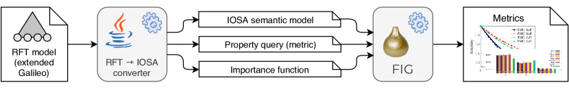
Figure 4: Tool chain

5.1 Extensions to Galileo

Standard Galileo supports exponential, log-normal, and Weibull pdfs. We use the keyword $\mathtt{EXT\_failPDF}$ to define arbitrary failure distributions. In LABEL:code:dormPDF, the $\mathsf{{SPARE}}$ gate ($\mathtt{Gate2}$) has its primary ($\mathtt{BE\_C}$) and one spare ($\mathtt{BE\_D}$), whose resp. fail pdfs are Rayleigh ($\sigma=0.06$) and exponential ($\lambda=0.0011$). We also allow the dormancy pdf of an $\mathsf{{SBE}}$ to be independent of its fail pdf. For this we add the $\mathtt{EXT\_dormPDF}$ keyword to define an arbitrary dormancy pdf. Thus we define the dormancy of $\mathtt{BE\_D}$ as an $\mathrm{Erlang}(k=3,\lambda=9)$ in LABEL:code:dormPDF. In the current implementation, a new time to failure is sampled (from the corresponding pdf) as the $\mathsf{{SBE}}$ is activated when the primary $\mathsf{{BE}}$ fails. This is a simplification since we work with potentially non-Markovian distributions; more realistic implementations are proposed as future work in Sec. 8.

⬇

toplevel "Gate2";

"Gate2" wsp "BE_C" "BE_D";

"BE_C" EXT_failPDF=rayleigh(6.0E-2);

"BE_D" lambda=1.11E-3 EXT_dormPDF=erlang(3,9);

Code 1: $\mathsf{{SBE}}$s and arbitrary pdfs in extended Galileo

Finally, we also extend Galileo with the keywords $\mathtt{repairbox\_priority}$ and $\mathtt{EXT\_repairPDF}$. These respectively define arbitrary repair policies for the $\mathsf{{RBOX}}$ elements, and the repair pdfs of $\mathsf{{BE}}$s and $\mathsf{{SBE}}$s. All $\mathsf{{BE}}$s in LABEL:code:repairPDF are repairable, with repair time uniformly distributed on the real intervals $[8,24]$ and $[8,12]$. The last line of the LABEL:code:repairPDF defines the $\mathsf{{RBOX}}$ of the system, which handles one repair at a time. Its repair policy determines which $\mathsf{{BE}}$ to choose when more than one is failed at the same time. For instance, if all $\mathsf{{BE}}$s fail and the $\mathsf{{RBOX}}$ “finishes repairing” $\mathtt{BE\_G}$, it will next repair $\mathtt{BE\_E}$ (before $\mathtt{BE\_F}$).

⬇

toplevel "Gate3";

"Gate3" and "BE_E" "BE_F" "BE_G";

"BE_E" lambda=6.0E-5 EXT_repairPDF=uniform(8,24);

"BE_F" lambda=7.0E-5 EXT_repairPDF=uniform(8,24);

"BE_G" lambda=6.0E-5 EXT_repairPDF=uniform(8,12);

"RB1" repairbox_priority "BE_E" "BE_F" "BE_G";

Code 2: Repairs in extended Galileo

5.2 Converter: RFT $\to$ IOSA

We also implemented the iosa semantics for rft [38]. For this we developed a Java textual converter whose input is an rft defined in extended Galileo. The converter outputs the iosa semantics of the tree, and the composition function for the corresponding local importance functions using Table 2.

Algorithm 1 Conversion from rft to iosa

1:procedure RFTtoIOSA($\mathit{in}$, $\mathit{out}$[3])

2:     $\mathit{rft}$ $\leftarrow$ parseRFT($\mathit{in}$)

3:     convertDynamicGates($\mathit{rft}$)

4:     $\mathit{cif}$ $\leftarrow$ templateImpFun($\mathit{rft}$)

5:     $\mathit{out}$[0] $\leftarrow$ convertTree($\mathit{rft}$)

6:     $\mathit{out}$[0] $\leftarrow$ convertRBOX($\mathit{rft}$, $\mathit{out}$[0])

7:     $\mathit{out}$[1] $\leftarrow$ generateProperties($\mathit{out}$[0])

8:     $\mathit{out}$[2] $\leftarrow$ generateImpFun($\mathit{cif}$, $\mathit{out}$[0])

9:end procedure

The conversion procedure is show as Algorithm 1. The ast parsed from the rft is first processed to convert the dynamic $\mathsf{{PAND}}$ and $\mathsf{{FDEP}}$ gates as described in Sec. 4.1. From the resulting tree we implement (a template of) the importance function following Table 2. Next, the iosa for each tree node is computed following [38]. Once all automata names were thus defined, the $\mathsf{{RBOX}}$ is built and added to the (now final) iosa semantics. Also the property queries (system unreliability and unavailability) are then defined. Finally, the importance function template is filled with the iosa automata names, and returned as a complete importance function.

Regarding the queries, unreliability and unavailability are encoded as variants of pctl [27] and csl [2] that FIG can take as input. For instance, say we want to estimate the unreliability of the rft defined in LABEL:code:repairPDF at $T=15.5$. If the converter defined the variable $\mathtt{count}$, internal to the iosa module corresponding to the $\mathtt{Gate3}$ $\mathsf{{AND}}$, then generateProperties() produces a pctl query as in LABEL:code:reliabilityProp.

⬇

properties

P( U<=15.5 Gate3.count==3)

endproperties

Code 3: Unreliability property query for LABEL:code:repairPDF

5.3 FIG: RES to estimate rare dependability metrics

The FIG tool was devised to study temporal logic queries of iosa models [10], described either in their native syntax or in the jani model exchange format [14]. Using res embedded in statistical model checking, FIG computes (arbitrary) cis that estimate the degree to which a model complies to a property specification.

FIG was designed for automatic res, implementing the algorithms from [12, 13] to derive an importance function from the system model. It can select an aggregation operator, to compose the local functions computed for the modules of the system. This, however, depends on the property query, and does not lead to high quality importance functions for fta, where the structure is in the tree and not in the query—see [10] and our discussion in Sec. 4.1.

FIG can also be input a composition function, to aggregate the local importance functions of the system modules. This is the feature used by our $\text{{rft}}\rightarrow{{\text{{iosa}}}}$ converter, as detailed in Sec. 5.2 Thus, from the iosa model and the importance function produced by our converter, FIG performs res to compute cis around the dependability metrics queried.

6 Experimental evaluation

6.1 General setup

Using our tool chain, we have verified the efficiency of the theory introduced in Sec. 4. We experimented on 26 repairable non-Markovian dfts using different simulation algorithms: 1. Standard Monte Carlo (smc); 2. restartwith thresholds selected via the Sequential Monte Carlo algorithm [10, 11] for different splitting values (rst-$n$ for $n=2,3,5,8,11$); 3. restartwith thresholds selected via the Expected Success algorithm [11] (rst-es); and 4. Fixed Effort [23, 11] for different number of runs performed in each importance region (fe-$n$ for $n=8,12,16,24,32$). res algorithms were implemented using the importance function defined in Table 2, by following the theory from [12, 13, 11] to choose thresholds and splitting values automatically.

We ran our experiments in two types of nodes of a SLURM cluster running 64-bit Linux (Ubuntu, kernel 3.13.0-168): korenvliet nodes have CPUs Intel^® Xeon^® E5-2630 v3 @ 2.40 GHz, and 64 GB of DDR4 @ 1600 MHz RAM memory; caserta has CPUs Intel^® Xeon^® E7-8890 v4 @ 2.20 GHz, and 2 TB of DDR4 @ 1866 MHz RAM memory.

6.2 Division of experimental instances

We experimented on seven case studies. These were originally Markovian and without repairs [21, 52, 25, 46]. To turn them into non-Markovian rfts we added $\mathsf{{RBOX}}$ elements and modified its fail and repair pdfs as detailed in Sec. 6.3. Moreover, to delineate the performance boost of our theory in the analysis of rare dependability metrics, we tested each case study in increasingly resilient configurations. For this, we parameterised them: a higher value of the parameter in a case study implies a more resilient system, i.e. smaller unavailability or unreliability values. The values of the parameters are given in Table 3 and described below. Figs. 8 and 9 show that, the rarer the metric, the more efficient our res implementation becomes w.r.t. smc.

Table 3: General overview of experimental setting

. ​Metric Casej
study      Difficulty Simulation
algorithms P. Est.$\big{(}$ TO. UN AVAILABILITY VOT 2 $8.47{\times}10^{\text{\hskip 0.5pt\raisebox{0.1pt}{-}}4}$ 5 m smc rst-$\{2,3,5,8,11\}$ 3 $1.94{\times}10^{\text{\hskip 0.5pt\raisebox{0.1pt}{-}}5}$ 30 m 4 $4.70{\times}10^{\text{\hskip 0.5pt\raisebox{0.1pt}{-}}7}$ 3 h HECS 1 $6.26{\times}10^{\text{\hskip 0.5pt\raisebox{0.1pt}{-}}3}$ 5 s smc rst-es rst-$\{2,5,8,11\}$ 2 $6.11{\times}10^{\text{\hskip 0.5pt\raisebox{0.1pt}{-}}5}$ 20 s 3 $1.56{\times}10^{\text{\hskip 0.5pt\raisebox{0.1pt}{-}}6}$ 2 m 4 $1.16{\times}10^{\text{\hskip 0.5pt\raisebox{0.1pt}{-}}7}$ 10 m 5 $2.02{\times}10^{\text{\hskip 0.5pt\raisebox{0.1pt}{-}}8}$ 1 h RC 3 $3.73{\times}10^{\text{\hskip 0.5pt\raisebox{0.1pt}{-}}5}$ 30 s smc rst-es rst-$\{2,5,8,11\}$ 4 $3.39{\times}10^{\text{\hskip 0.5pt\raisebox{0.1pt}{-}}6}$ 5 m 5 $5.07{\times}10^{\text{\hskip 0.5pt\raisebox{0.1pt}{-}}7}$ 30 m 6 $1.02{\times}10^{\text{\hskip 0.5pt\raisebox{0.1pt}{-}}7}$ 2 h RWC 1 $4.88{\times}10^{\text{\hskip 0.5pt\raisebox{0.1pt}{-}}4}$ 30 s smc rst-$\{2,5,8,11\}$ 2 $3.15{\times}10^{\text{\hskip 0.5pt\raisebox{0.1pt}{-}}5}$ 5 m 3 $3.03{\times}10^{\text{\hskip 0.5pt\raisebox{0.1pt}{-}}6}$ 30 m 4 $4.55{\times}10^{\text{\hskip 0.5pt\raisebox{0.1pt}{-}}7}$ 2 h UN RELIABILITY DSPARE 3 $7.03{\times}10^{\text{\hskip 0.5pt\raisebox{0.1pt}{-}}4}$ 5 m smc rst-$\{2,3,5,8,11\}$ fe-$\{8,16,32\}$ 4 $6.08{\times}10^{\text{\hskip 0.5pt\raisebox{0.1pt}{-}}5}$ 30 m 5 $7.31{\times}10^{\text{\hskip 0.5pt\raisebox{0.1pt}{-}}6}$ 3 h HECS 2 $1.98{\times}10^{\text{\hskip 0.5pt\raisebox{0.1pt}{-}}3}$ 20 s smc rst-$\{2,5,8,11\}$ fe-$\{8,16,32\}$ 3 $3.60{\times}10^{\text{\hskip 0.5pt\raisebox{0.1pt}{-}}5}$ 5 m 4 $2.35{\times}10^{\text{\hskip 0.5pt\raisebox{0.1pt}{-}}6}$ 30 m 5 $2.61{\times}10^{\text{\hskip 0.5pt\raisebox{0.1pt}{-}}7}$ 3 h FTPP (triad) 4 $1.20{\times}10^{\text{\hskip 0.5pt\raisebox{0.1pt}{-}}2}$ 30 s smc rst-$\{2,5\}$ fe-$\{8,12,16,24\}$ 5 $2.49{\times}10^{\text{\hskip 0.5pt\raisebox{0.1pt}{-}}4}$ 4 m 6 $6.34{\times}10^{\text{\hskip 0.5pt\raisebox{0.1pt}{-}}7}$ 40 m HVC 4 $1.11{\times}10^{\text{\hskip 0.5pt\raisebox{0.1pt}{-}}2}$ 90 s smc rst-$\{2,5,8,11\}$ fe-$8$ 5 $4.61{\times}10^{\text{\hskip 0.5pt\raisebox{0.1pt}{-}}4}$ 5 m 6 $3.44{\times}10^{\text{\hskip 0.5pt\raisebox{0.1pt}{-}}5}$ 30 m 7 $4.17{\times}10^{\text{\hskip 0.5pt\raisebox{0.1pt}{-}}6}$ 2 h RWC 2 $7.03{\times}10^{\text{\hskip 0.5pt\raisebox{0.1pt}{-}}4}$ 5 m smc rst-$\{2,5,8,11\}$ 3 $6.08{\times}10^{\text{\hskip 0.5pt\raisebox{0.1pt}{-}}5}$ 30 m 4 $7.31{\times}10^{\text{\hskip 0.5pt\raisebox{0.1pt}{-}}6}$ 2 h

For each parametric case study we compare the simulation algorithms mentioned above. We estimate system unavailability and unreliability at time $T=10^{3}$. For each combination of metric, fault tree, and algorithm—an instance—we computed cis of 95% confidence level around the point estimate for the metric. To do so, we ran simulations with FIG for predefined wall-clock runtimes (that depend on the case and parameter as detailed in Table 3), and built 10 cis for each instance.  We then compared the average width of the cis per instance. The algorithm with the most precise (narrowest) intervals was the most efficient to compute that metric on that tree. In Sec. 6.4 we show that for the most resilient configurations of all case studies, res algorithms implemented from our importance functions are more efficient (and as automatic) than smc.

An overview of the full experimental setting is given in Table 3. The parameterised configurations of all case studies are detailed in Difficulty. Its sub-columns are: [ P. ] that gives the parameter value of each case study—see Sec. 6.3; [ TO. ] for “Time-Out,” i.e. the simulation runtime, higher for the more resilient configurations of a case study to let the algorithms sample some rare event; and [ Est. ] that gives the point estimate averaged over all values, ranging over all simulation algorithms and the 10 (repeated and independent) computations performed for each tree and metric.

Note that the Time-Out chosen for a (parameterised) case study may be insufficient for certain algorithms to observe any rare event, e.g. for smc. If that happens, the stochastic model checker FIG reports a “null estimate” $[0,0]$. Moreover, the simulation of random events depend on the rng—and the seed—used by FIG, so different runs may yield different cis. To account for these factors when assessing the outcome of each instance, we computed each ci 10 times. This gives us three dimensions to assess the performance of an algorithm in an instance: (i ) how many times did it yield a not-null estimate, (ii ) what was the average width of the resulting cis for that case study and parameter (considering not-null estimates only), and (iii ) what was the variance of those widths.

For example, running simulations for 2 minutes, we estimated the unavailability of the parameterised case study “HECS-3.​​” Using smc we computed 10 independent cis. The same was done for each of rst-2,5,8,11,es. Results are shown as whisker-bar plots in Sec. 6.4. Each bar corresponds to the cis computed for an instance, i.e. a specific algorithm on one case study with certain parameter. The height of the bar is the mean ci width for the 10 iterations of the algorithm (discarding null estimates). The whiskers on top of it are the standard deviation of these widths, and a bold number at its base (e.g.   3 10  ) indicates how many iterations of algo yielded not-null estimates.

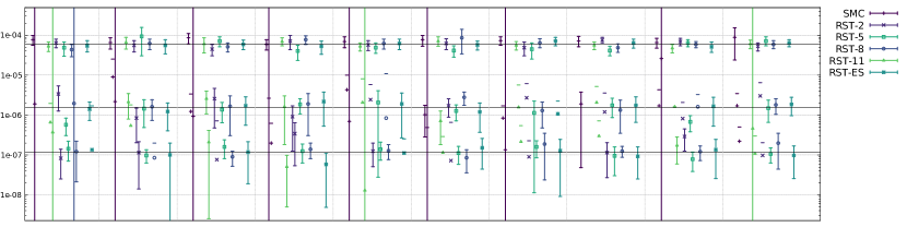
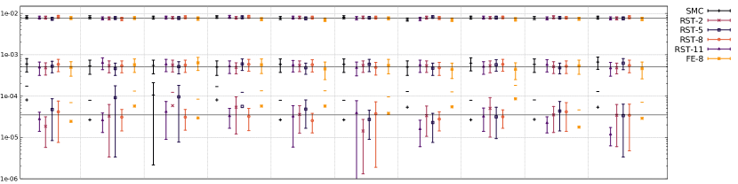
Figure 5: cis for unavailability of HECS

Figure 6: cis for unreliability of HVC

The cis themselves—whose width we compare in Sec. 6.4—for unavailability of HECS-2, HECS-3, and HECS-4, are shown in Fig. 6. The three horizontal lines are their corresp. unavailability values: $6.11{\times}10^{\text{\hskip 0.5pt\raisebox{0.1pt}{-}}5}$, $1.56{\times}10^{\text{\hskip 0.5pt\raisebox{0.1pt}{-}}6}$, and $1.16{\times}10^{\text{\hskip 0.5pt\raisebox{0.1pt}{-}}7}$. Here we tested algorithms smc, rst-es, and rst-$\{2,5,8,11\}$. To explore res diversity, yet keep the amount of experimentation manageable, in other cases we tested different algorithms—see Table 3.

The 10 cis computed per instance are separated in Fig. 6 by vertical gray dashed lines. The cis are the coloured vertical error-bars. Some of them are the trivial real interval $[0,1]$ and appear as vertical coloured lines; e.g. all iterations of smc for HECS-4 except for the 4^th, 8^th, and 10^th. Sometimes only one extreme of the interval is not trivial, e.g. the 4^th and 10^th iterations of smc for HECS-4 which respectively yielded $[0,6.31{\times}10^{\text{\hskip 0.5pt\raisebox{0.1pt}{-}}7}]$ and $[0,5.07{\times}10^{\text{\hskip 0.5pt\raisebox{0.1pt}{-}}7}]$. When not even a point estimate was computed for an iteration, the ci is missing completely from the plot, e.g. the 8^th iteration of smc for HECS-4.

Fig. 6 shows the cis computed in the same way for unreliability of the HVC case study. In this case we experimented with the algorithms smc, fe-8, and rst-$\{2,5,8,11\}$. It can be seen that for HVC-6 (the downmost horizontal line at $3.44{\times}10^{\text{\hskip 0.5pt\raisebox{0.1pt}{-}}5}$) only the third iteration of smc yielded a complete ci, and it is very wide. In contrast, algorithms like rst-2 and rst-8 always converged to reasonable ci estimates in 30 m of simulation runtime for this system configuration. This is the trend with all experiments: as expected, the more rare the metric, the wider the cis computed in the time limit via smc, and at some point it becomes infeasible to converge to non-trivial cis. In contrast, res algorithms—implemented from our importance function—can still compute cis in the most extreme situations experimented with our case studies. This is conveyed in Sec. 6.4 via whisker-bar plots, that show the average width of cis achieved per instance.

6.3 The case studies

We briefly describe the seven parametric case studies: VOT and DSPARE were devised for this work, to check whether res is efficient on such tree structure and probe different simulation runtime limits; FTPP and HECS were taken from the literature on fta [21, 52]; and RC, HVC, and RWC concern industrial railroad systems [26, 25, 46]. The structure of all these systems is presented in Fig. 7; the fail, repair, and dormancy pdfs of their $\mathsf{{BE}}$s and $\mathsf{{SBE}}$s are given in Table 4.

Figure 7: Case studies used for experimentation

(a) VOT

 

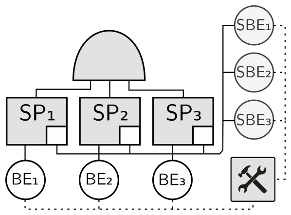
(b) DSPARE

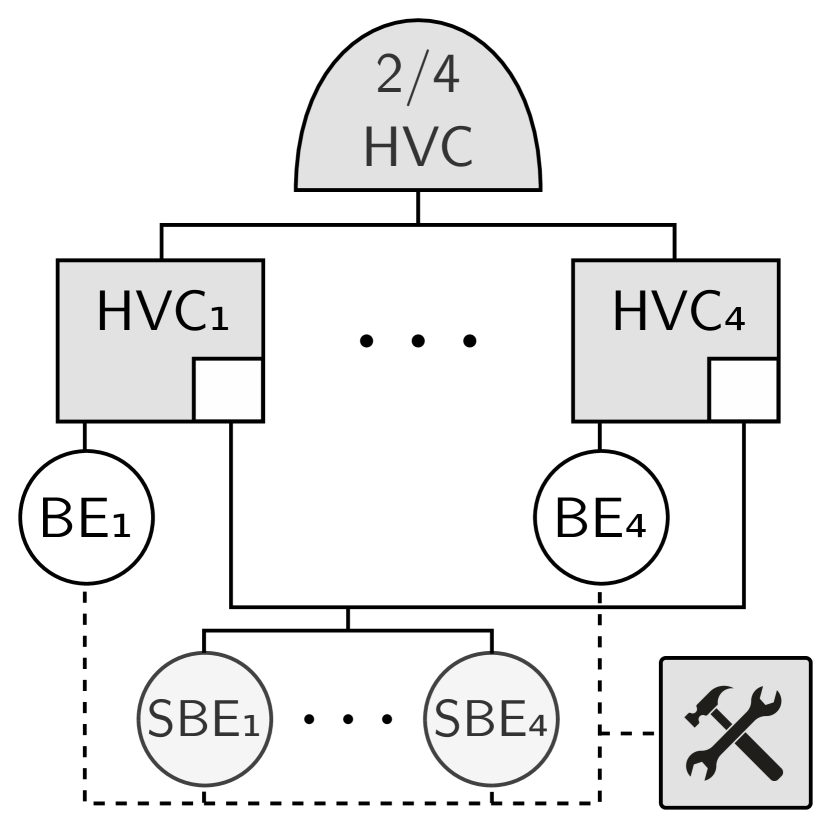
(c) HVC

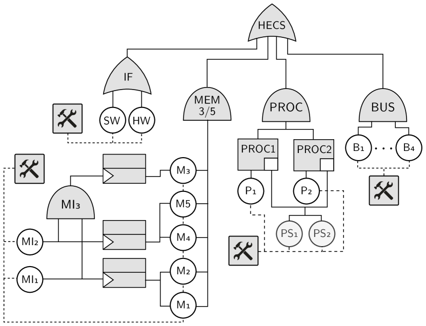
(d) HECS

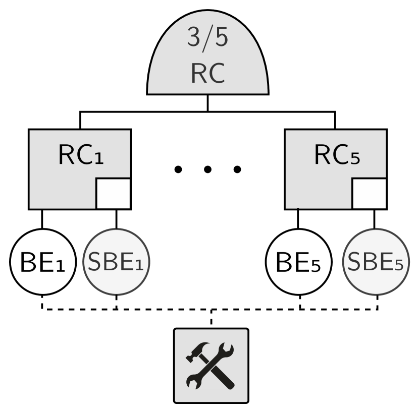
(e) RC

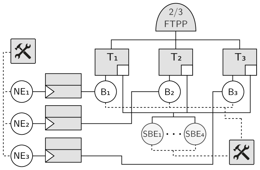
(f) FTPP

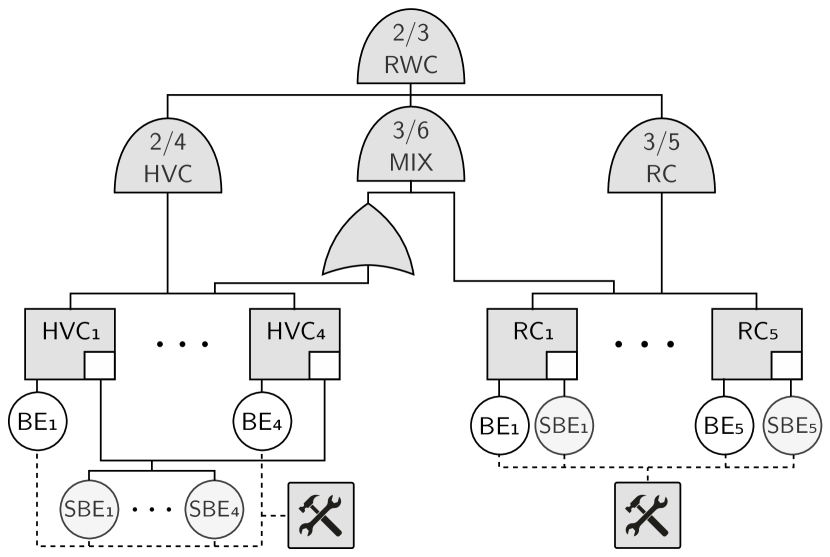
(g) RWC

VOT

(Fig. 7(a))   The first case study is a binary $\mathsf{{AND}}$ gate whose children are $\mathsf{{VOT}}$ gates, whose children are basic elements. All $\mathsf{{BE}}$s are connected to a single $\mathsf{{RBOX}}$, which first repairs children of $\mathsf{{VOT}}$-$A$ and, if all are operational, then repairs any failed child of $\mathsf{{VOT}}$-$B$. $\mathsf{{VOT}}$-$A$ is a $\mathsf{{VOT}}_{k_{A}}$ gate with $n_{A}$ children, and analogously for $\mathsf{{VOT}}$-$B$, where $n_{A}=n_{B}-1$, $k_{A}=n_{A}-3$, and $k_{B}=n_{B}-2$. From the $n_{A}$ children of $\mathsf{{VOT}}$-$A$, $n_{B}-4$ $\mathsf{{BE}}$s are also children of $\mathsf{{VOT}}$-$B$. VOT is parameterised on $n_{B}=8,9,10$ resp. for VOT-$\{2,3,4\}$. Thus in VOT-2 in Fig. 7(a), $\mathsf{{VOT}}$-$A$ is a $\mathsf{{VOT}}_{4}$ with $7$ children, and $\mathsf{{VOT}}_{B}$ is a $\mathsf{{VOT}}_{6}$ with $8$ children.

DSPARE

(Fig. 7(b))   This is a ternary $\mathsf{{AND}}$ gate whose children are $\mathsf{{SPARE}}$ gates, whose children are basic elements. $\mathsf{{SBE}}$s are shared among all $\mathsf{{SPARE}}$s: each gate has a unique primary $\mathsf{{BE}}$ and $n$ spare $\mathsf{{BE}}$s. The parameterisation is on $n\in\{3,4,5\}$: Fig. 7(b) shows DSPARE-3. All basic elements are connected to a single $\mathsf{{RBOX}}$, whose priority is to first repair failed $\mathsf{{SBE}}$s and, if all are operational, then repair failed $\mathsf{{BE}}$s.

HECS

(Fig. 7(d))   The Hypothetical Example Computer System is a classic case study from fta literature [52]. We study the variant with two memory-unit interfaces, that affect the memory banks via functional dependencies. Furthermore, we define one $\mathsf{{RBOX}}$ for each subsystem: Interface, Memory, Processors, and Bus. HECS is parameterised on the number of parallel buses ($\mathsf{{BE}}$s $\mathsf{B_{k}}$) and shared spare processors ($\mathsf{{SBE}}$s $\mathsf{PS_{b}}$). For $n\in\{1,2,3,4,5\}$ HECS-$n$ has $n$ shared spare processors and $2\,n$ parallel buses; Fig. 7(d) depicts HECS-2.

FTPP

(Fig. 7(f))   The Fault Tolerant Parallel Processor is another classic ft. We implemented the grouped cold-spare variant from [21], where all triads depend on all network elements, and there is an independent $\mathsf{{SBE}}$ per triad. We study an individual triad: the tree root is thus a $\mathsf{{VOT}}_{2}$ with 3 $\mathsf{{SPARE}}$s as children—see Fig. 7(f). We defined independent repair boxes for the network and processing elements; the $\mathsf{{RBOX}}$ in charge of processors prioritises the repair of primary $\mathsf{{BE}}$s. FTPP is parameterised on the number of (shared) $\mathsf{{SBE}}$s of the triad. For $n\in\{4,5,6\}$ FTPP-$n$ has $n$ shared $\mathsf{{SBE}}$s; Fig. 7(f) depicts FTPP-4.

RC

(Fig. 7(e))   The Relay Cabinets subsystem is one of the components of the railways cabinets example in Fig. 2. It is a $\mathsf{{VOT}}_{k}$ gate with $k+2$ children: $\mathsf{{SPARE}}$s with one (independent) $\mathsf{{SBE}}$ besides their primary $\mathsf{{BE}}$. There is a single $\mathsf{{RBOX}}$ for all basic elements, which prioritises repairs of primary $\mathsf{{BE}}$s. RC is parameterised in the number of $\mathsf{{SPARE}}$s that need to fail to cause a top event: $k\in\{3,4,5,6\}$; Fig. 7(e) depicts RC-3.

HVC

(Fig. 7(c))   High Voltage Cabinets is the other main component of the railways cabinet example. This is a $\mathsf{{VOT}}_{2}$ gate with 4 $\mathsf{{SPARE}}$ children. Here however the $\mathsf{{SBE}}$s are shared among all $\mathsf{{SPARE}}$s: HVC is parameterised in the amount of these $\mathsf{{SBE}}$s, $n\in\{4,5,6,7\}$, with Fig. 7(c) depicting HVC-4. The single $\mathsf{{RBOX}}$ is analogous to the one in RC.

RWC

(Fig. 7(g))   The full Railways Cabinet case study combines RC and HVC with a $\mathsf{{VOT}}$. The $\mathsf{{SPARE}}$s of RC are direct children of this gate, whereas the high voltage cabinets are interfaced via an $\mathsf{{OR}}$. The parameterisation of RWC, $m\in\{1,2,3,4\}$, combines those of its subsystems. RWC-$m$ uses RC-$(m+1)$ and HVC-$(m+2)$; Fig. 7(g) depicts RWC-2.

Table 4: Basic elements of the case studies

Basic element	Fail time pdf	Rep. pdf	Dorm. pdf
VOT:$\big{(}\!$
$\mathsf{{BE}}$-$A$	$\mathrm{lnor}(4.37,0.33)$	$\mathrm{uni}(0.4,0.95)$
$\mathsf{{BE}}$-$B$	$\mathrm{wei}(4.5,0.0125)$	$\mathrm{uni}(0.4,0.95)$
DSPARE:$\big{(}\!$
$\mathsf{{BE}}$	$\mathrm{exp}(0.07)$	$\mathrm{uni}(1.0,2.0)$
$\mathsf{{SBE}}$	$\mathrm{exp}(0.07)$	$\mathrm{uni}(1.0,2.0)$	$\mathrm{exp}(0.035)$
HECS:$\big{(}\!$
$\mathsf{SW}$	$\mathrm{exp}(4.5{\times}10^{\text{\hskip 0.5pt\raisebox{0.1pt}{-}}12})$	$\mathrm{uni}(28.0,56.0)$
$\mathsf{HW}$	$\mathrm{exp}(1.0{\times}10^{\text{\hskip 0.5pt\raisebox{0.1pt}{-}}10})$	$\mathrm{uni}(28.0,56.0)$
$\mathsf{MI_{i}}$	$\mathrm{exp}(5.0{\times}10^{\text{\hskip 0.5pt\raisebox{0.1pt}{-}}9})$	$\mathrm{uni}(21.0,28.0)$
$\mathsf{M_{j}}$	$\mathrm{exp}(6.0{\times}10^{\text{\hskip 0.5pt\raisebox{0.1pt}{-}}8})$	$\mathrm{uni}(21.0,28.0)$
$\mathsf{B_{k}}$	$\mathrm{exp}(8.7{\times}10^{\text{\hskip 0.5pt\raisebox{0.1pt}{-}}4})$	$\mathrm{lnor}(4.45,0.24)$
$\mathsf{P_{a}}$	$\mathrm{exp}(1.0{\times}10^{\text{\hskip 0.5pt\raisebox{0.1pt}{-}}3})$	$\mathrm{lnor}(4.45,0.24)$
$\mathsf{PS_{b}}$	$\mathrm{exp}(1.5{\times}10^{\text{\hskip 0.5pt\raisebox{0.1pt}{-}}3})$	$\mathrm{lnor}(4.45,0.24)$	$\mathrm{dir}(\aleph)$
FTPP:$\big{(}\!$
$\mathsf{NE_{i}}$	$\mathrm{lnor}(6.5,0.5)$	$\mathrm{nor}(150.0,50.0)$
$\mathsf{B_{j}}$	$\mathrm{exp}(2.8{\times}10^{\text{\hskip 0.5pt\raisebox{0.1pt}{-}}2})$	$\mathrm{nor}(15.0,3.0)$
$\mathsf{{SBE}}_{k}$	$\mathrm{exp}(2.8{\times}10^{\text{\hskip 0.5pt\raisebox{0.1pt}{-}}2})$	$\mathrm{nor}(15.0,3.0)$	$\mathrm{dir}(\aleph)$
RC:$\big{(}\!$
$\mathsf{{BE}}_{i}$	$\mathrm{exp}(0.04)$	$\mathrm{nor}(2.0,0.7)$
$\mathsf{{SBE}}_{j}$	$\mathrm{exp}(0.04)$	$\mathrm{nor}(2.0,0.7)$	$\mathrm{exp}(0.5)$
HVC:$\big{(}\!$
$\mathsf{{BE}}_{i}$	$\mathrm{ray}(1.999)$	$\mathrm{uni}(0.15,0.45)$
$\mathsf{{SBE}}_{j}$	$\mathrm{ray}(1.999)$	$\mathrm{uni}(0.15,0.45)$	$\mathrm{erl}(3.0,0.25)$

Abbrev:	Distribution:
$\mathrm{dir}(x)$	$\mathrm{Dirac}(x)$
$\mathrm{exp}(\lambda)$	$\mathrm{exponential}(\lambda)$
$\mathrm{erl}(k,\lambda)$	$\mathrm{Erlang}(k,\lambda)$
$\mathrm{uni}(a,b)$	$\mathrm{uniform}([a,b]_{\mathbb{R}})$
$\mathrm{ray}(\sigma)$	$\mathrm{Rayleigh}(\sigma)$
$\mathrm{wei}(k,\lambda)$	$\mathrm{Weibull}(k,\lambda)$
$\mathrm{nor}(\mu,\sigma)$	$\mathrm{normal}(\mu,\sigma)$
$\mathrm{lnor}(\mu,\sigma)$	$\mathrm{log\text{-}normal}(\mu,\sigma)$

6.4 Results of experimentation: comparing CI widths

Figure 8: ci precision for system unavailability

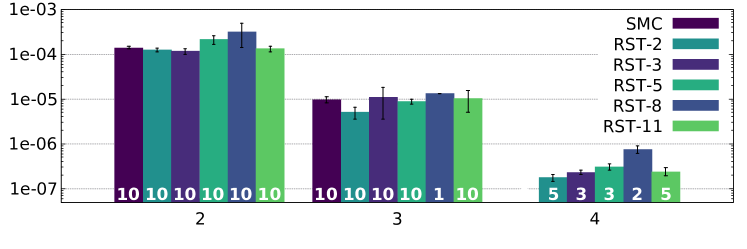
(a) VOT

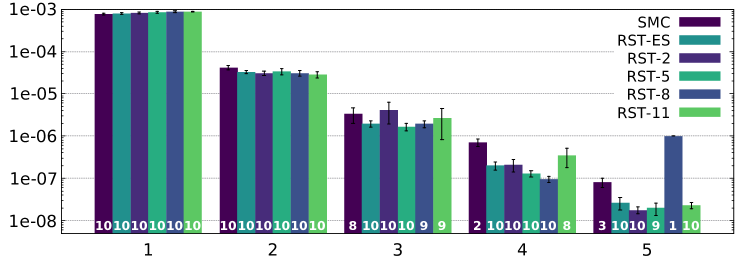
(b) HECS

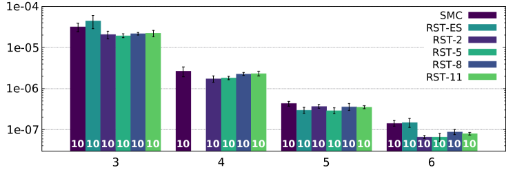
(c) RC

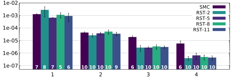
(d) RWC

Using smc and restart we computed $\mathrm{UNAVA}$ for VOT-$\{2,3,4\}$, HECS-$\{1,2,3,4,5\}$, RC-$\{3,4,5,6\}$, and RWC-$\{1,2,3,4\}$. fe was not used since it requires regeneration theory for steady-state analysis [23], which is not always feasible with non-Markovian models. The mean widths of the cis achieved per instance (ulting 95% confidence level) are shown in Fig. 8.

For example for VOT-2 (Fig. 8(a)), 10 independent computations with smc ran in caserta for 5 min, and all converged to not-null cis (  10  ). The mean width of these cis was $1.40{\times}10^{\text{\hskip 0.5pt\raisebox{0.1pt}{-}}4}$ and their standard deviation $7.96{\times}10^{\text{\hskip 0.5pt\raisebox{0.1pt}{-}}6}$. For VOT-3, all smc computations yielded not-null cis (after 30 min) with an average precision of $9.62{\times}10^{\text{\hskip 0.5pt\raisebox{0.1pt}{-}}6}$ and standard deviation $1.52{\times}10^{\text{\hskip 0.5pt\raisebox{0.1pt}{-}}6}$. For VOT-4 all smc simulations yielded null cis after 3 hours of simulation. Instead, rst-2 converged to 10, 10, and 5 not-null cis resp. for VOT-{2,3,4}, with mean widths (and standard deviation): $1.24{\times}10^{\text{\hskip 0.5pt\raisebox{0.1pt}{-}}4}$ ($1.19{\times}10^{\text{\hskip 0.5pt\raisebox{0.1pt}{-}}5}$), $5.09{\times}10^{\text{\hskip 0.5pt\raisebox{0.1pt}{-}}6}$ ($1.48{\times}10^{\text{\hskip 0.5pt\raisebox{0.1pt}{-}}6}$), and $1.79{\times}10^{\text{\hskip 0.5pt\raisebox{0.1pt}{-}}7}$ ($3.19{\times}10^{\text{\hskip 0.5pt\raisebox{0.1pt}{-}}8}$). Thus for the VOT case study, rst-2 was consistently more efficient than smc, and the efficiency gap increased as $\mathrm{UNAVA}$ became rarer.

This trend repeats in all experiments: as expected, the rarer the metric, the wider the cis computed in the time limit, until at some point it becomes very hard to converge to not-null cis at all (specially for smc). For the least resilient configuration of each case study, smc can be competitive or even more efficient than some isplit variants. For instance for VOT-1 and HECS-1 in Figs. 8(a) and 8(b), all computations converged to not-null cis for all algorithms, but smc exhibits less variable ci widths, viz. smaller whiskers. This is reasonable: truncating and splitting traces in restart adds (i ) simulation overhead that may not pay off to estimate not-so-rare events, and on top of it (ii ) correlations of cloned traces that share a common history, increasing the variability among independent runs. On the other hand and as expected, smc looses this competitiveness for all case studies as failures become rarer, here when $\mathrm{UNAVA}\leqslant 1.0{\times}10^{\text{\hskip 0.5pt\raisebox{0.1pt}{-}}5}$. This holds nicely for the biggest case studies: HECS-5​​​(a 42-nodes rft whose iosa has 126-not-clock variables $\approx 2.89{\times}10^{\text{\hskip 0.5pt\raisebox{0.1pt}{}}38}$ states, with 57 clocks of exponential, uniform, and log-normal pdfs) and RWC-4 (42 nodes, 181 variables $\approx 6.93{\times}10^{\text{\hskip 0.5pt\raisebox{0.1pt}{}}73}$ states, 62 clocks of exponential, Erlang, Rayleigh, uniform, and normal pdfs).

We also estimated the $\mathrm{UNREL}_{1000}$ of DSPARE-{3,4,5}, RWC-{2,3,4}, FTPP-{4,5,6}, HVC-{4,…,7}, and HECS-{2,…,5} using smc, restart, and fe. For HVC (only) we ran 20 experiments per tree, 10 in each cluster node. Fig. 9 shows the results.

Figure 9: ci precision for system unreliability

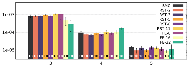
(a) DSPARE

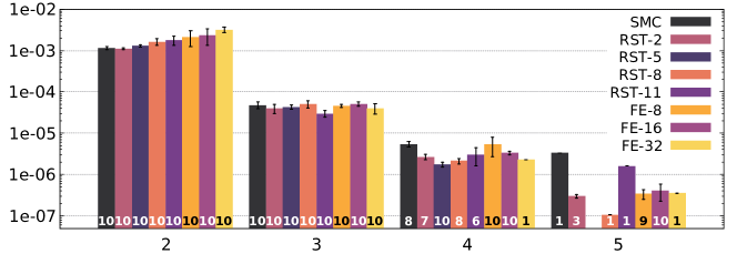
(b) HECS

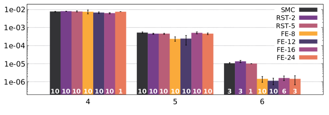
(c) FTPP

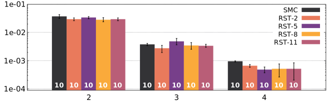
(d) RWC

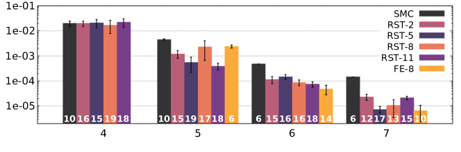
(e) HVC

The overall trend shown for unreliability estimations is similar to the previous unavailability cases. Here however it was possible to use Fixed Effort, since every simulation has a clearly defined end at time $T=10^{3}$. It is interesting thus to compare the efficiency of restart vs. fe: we note for example that some variants of fe performed considerably better than any other approach in the most resilient configurations of FTPP and HECS. It is nevertheless difficult to draw general conclusions from Figs. 9(a) to 9(b), since some variants that performed best in a case study—e.g. fe-16 in HECS—did worse in others—e.g. FTPP, where the best algorithms were fe-8,12. Furthermore, fe-8, which is always better than smc when $\mathrm{UNREL}_{1000}<10^{-3}$, did not perform very well in HVC, where the algorithms that achieved the narrowest and most not-null cis were rst-5,11. Such cases notwithstanding, fe is a solid competitor of restart in our benchmark.

Another relevant point of study is the optimal effort $e$ for rst-e or fe-e, which shows no clear trend in our experiments. Here, $e$ is a “global effort” used by these algorithms, equal for all $\pazocal{S}_{k}$ regions. $e$ also alters the way in which the thresholds selection algorithm Sequential Monte Carlo (seq [13]) selects the $\ell_{k}$. The lack of guidelines to select a value for $e$ that works well across different systems was raised in [10]. This motivated the development of Expected Success (es [11]), which selects efforts individually per $\pazocal{S}_{k}$ (or $\ell_{k}$). Thus, in rst-es, a trace up-crossing threshold $\ell_{k}$ is split according to the individual effort $e_{k}$ selected by es. In the benchmark of [11], which consists mostly of queueing systems, es was shown superior to seq. However, experimental outcomes on dfts in this work are different: for $\mathrm{UNAVA}$, rst-es yielded mildly good results for HECS and RC; for the other case studies and for all $\mathrm{UNREL}_{1000}$ experiments, rst-es always yielded null cis. It was found that the effort selected for most thresholds $\ell_{k}$ was either too small—so splitting in $e_{k}$ was not enough for the rst-es trace to reach $\ell_{k+1}$—or too large—so there was a splitting/truncation overhead. This point is further addressed in the conclusions.

Beyond comparisons among the specific algorithms, be these for res or for selecting thresholds, it seems clear that our approach to fta via isplit deploys the expected results. For each parameterised case study ${\pazocal{CS}}_{\mathfrak{p}}$, we could find a value of the parameter $\mathfrak{p}$ where the level of resilience is such, that smc is less efficient than our automatically-constructed isplit framework. This is particularly significant for big dfts like HECS and RWC, whose complex structure could be exploited by our importance function.

7 Related work

Most work on dft analysis assumes discrete [52, 4] or exponentially distributed [17, 35] components failure. Furthermore, components repair is seldom studied in conjunction with dynamic gates [7, 4, 48, 35, 37]. In this work we address repairable dfts, whose failure and repair times can follow arbitrary pdfs. More in detail, rfts were first formally introduced as stochastic Petri nets in [7, 40]. Our work stands on [38], which reviews [40] in the context of stochastic automata with arbitrary pdfs. In particular we also address non-Markovian continuous distributions: in Sec. 6 we experimented with exponential, Erlang, uniform, Rayleigh, Weibull, normal, and log-normal pdfs. Furthermore and for the first time, we consider the application of [40, 38] to study rare events.

Much effort in res has been dedicated to study highly reliable systems, deploying either importance splitting or sampling. Typically, importance sampling can be used when the system takes a particular shape. For instance, a common assumption is that all failure (and repair) times are exponentially distributed with parameters $\lambda^{i}$, for some $\lambda\in\mathbb{R}$ and $i\in\mathbb{N}_{>0}$. In these cases, a favourable change of measure can be computed analytically [24, 28, 39, 41, 58, 47].

In contrast, when the fail/repair times follow less-structured distributions, importance splitting is more easily applicable. As long as a full system failure can be broken down into several smaller components failures, an importance splitting method can be devised. Of course, its efficiency relies heavily on the choice of importance function. This choice is typically done ad hoc for the model under study [53, 36, 55]. In that sense [30, 31, 12, 13] are among the first to attempt a heuristic derivation of all parameters required to implement splitting. This is based on formal specifications of the model and property query (the dependability metric). Here we extended [12, 13, 10], using the structure of the fault tree to define composition operands. With these operands we aggregate the automatically-computed local importance functions of the tree nodes. This aggregation results in an importance function for the whole model.

8 Conclusions

We have presented a theory to deploy automatic importance splitting (isplit) for fault tree analysis of repairable dynamic fault trees (rfts). This Rare Event Simulation approach supports arbitrary probability distributions of components failure and repair. The core of our theory is an importance function $\pazocal{I}_{\triangle}$ defined structurally on the tree. From such function we implemented isplit algorithms, and used them to estimate the unreliability and unavailability of highly-resilient rfts. Departing from classical approaches, that define importance functions ad hoc using expert knowledge, our theory computes all metadata required for res from the model and metric specifications. Nonetheless, we have shown that for a fixed simulation time budget and in the most resilient rfts, diverse isplit algorithms can be automatically implemented from $\pazocal{I}_{\triangle}$, and always converge to narrower confidence intervals than standard Monte Carlo simulation.

There are several paths open for future development. First and foremost, we are looking into new ways to define the importance function, e.g. to cover more general categories of fts such as fault maintenance trees [44]. It would also be interesting to look into possible correlations among specific res algorithms and tree structures, that yield the most efficient estimations for a particular metric. Moreover, we have defined $\pazocal{I}_{\triangle}$ based on the tree structure alone. It would be interesting to further include stochastic information in this phase, and not only afterwards during the thresholds-selection phase.

Regarding thresholds, the relatively bad performance of the Expected Success algorithm shows a spot for improvement. In general, we believe that enhancing its statistical properties should alleviate the behaviour mentioned in Sec. 6.4. Moreover, techniques to increase trace independence during splitting (e.g. resampling) could further improve the performance of the isplit algorithms. Finally, we are investigating enhancements in iosa and our tool chain, to exploit the ratio between fail and dormancy pdfs of $\mathsf{{SBE}}$s in warm $\mathsf{{SPARE}}$ gates.

References

- [1] Abate, A., Budde, C.E., Cauchi, N., Hoque, K.A., Stoelinga, M.: Assessment of maintenance policies for smart buildings: Application of formal methods to fault maintenance trees. PHM Society European Conference 4(1) (2018)
- [2] Baier, C., Katoen, J., Hermanns, H.: Approximate symbolic model checking of continuous-time markov chains. In: CONCUR 1999. pp. 146–161 (1999). https://doi.org/10.1007/3-540-48320-9_12
- [3] Bayes, A.J.: Statistical techniques for simulation models. Australian computer journal 2(4), 180–184 (1970)
- [4] Beccuti, M., Raiteri, D., Franceschinis, G., Haddad, S.: Non deterministic repairable fault trees for computing optimal repair strategy. In: VALUETOOLS 2008 (2010). https://doi.org/10.4108/ICST.VALUETOOLS2008.4411
- [5] Blanchet, J., Mandjes, M.: Rare event simulation for queues. In: Rubino and Tuffin [43], pp. 87–124. https://doi.org/10.1002/9780470745403.ch5
- [6] Blom, H.A.P., Bakker, G.J.B., Krystul, J.: Rare event estimation for a large-scale stochastic hybrid system with air traffic application. In: Rubino and Tuffin [43], pp. 193–214. https://doi.org/10.1002/9780470745403.ch9
- [7] Bobbio, A., Raiteri, D.: Parametric fault trees with dynamic gates and repair boxes. In: RAMS’04. pp. 459–465 (2004). https://doi.org/10.1109/RAMS.2004.1285491
- [8] Boudali, H., Crouzen, P., Haverkort, B.R., Kuntz, M., Stoelinga, M.: Architectural dependability evaluation with arcade. In: DSN’08. pp. 512–521 (2008). https://doi.org/10.1109/DSN.2008.4630122
- [9] Boudali, H., Dugan, J.B.: A new bayesian network approach to solve dynamic fault trees. In: Annual Reliability and Maintainability Symposium, 2005. Proceedings. pp. 451–456 (2005). https://doi.org/10.1109/RAMS.2005.1408404
- [10] Budde, C.E.: Automation of Importance Splitting Techniques for Rare Event Simulation. Ph.D. thesis, Universidad Nacional de Córdoba, Córdoba, Argentina (2017)
- [11] Budde, C.E., D’Argenio, P.R., Hartmanns, A.: Better automated importance splitting for transient rare events. In: SETTA. LNCS, vol. 10606, pp. 42–58. Springer (2017)
- [12] Budde, C.E., D’Argenio, P.R., Hermanns, H.: Rare event simulation with fully automated importance splitting. In: EPEW 2015. LNCS, vol. 9272, pp. 275–290. Springer (2015). https://doi.org/10.1007/978-3-319-23267-6_18
- [13] Budde, C.E., D’Argenio, P.R., Monti, R.E.: Compositional construction of importance functions in fully automated importance splitting. In: VALUETOOLS 2016. pp. 30–37 (2017). https://doi.org/10.4108/eai.25-10-2016.2266501
- [14] Budde, C.E., Dehnert, C., Hahn, E.M., Hartmanns, A., Junges, S., Turrini, A.: JANI: Quantitative model and tool interaction. In: TACAS. LNCS, vol. 10206, pp. 151–168. Springer (2017). https://doi.org/10.1007/978-3-662-54580-5_9
- [15] Coppit, D., Sullivan, K.J., Dugan, J.B.: Formal semantics of models for computational engineering: a case study on dynamic fault trees. In: ISSRE 2000. pp. 270–282 (2000). https://doi.org/10.1109/ISSRE.2000.885878
- [16] Coppit, D., Sullivan, K.J.: Galileo: A tool built from mass-market applications. In: Software Engineering, 2000. Proceedings of the 2000 International Conference on. pp. 750–753. IEEE (2000)
- [17] Crouzen, P., Boudali, H., Stoelinga, M.: Dynamic fault tree analysis using input/output interactive markov chains. In: DSN 2007. pp. 708–717 (2007). https://doi.org/10.1109/DSN.2007.37
- [18] D’Argenio, P.R., Lee, M.D., Monti, R.E.: Input/output stochastic automata - compositionality and determinism. In: FORMATS 2016. LNCS, vol. 9884, pp. 53–68 (2016). https://doi.org/10.1007/978-3-319-44878-7_4
- [19] D’Argenio, P.R., Monti, R.E.: Input/Output Stochastic Automata with Urgency: Confluence and weak determinism. In: ICTAC. LNCS, vol. 11187, pp. 132–152. Springer (2018). https://doi.org/10.1007/978-3-030-02508-3_8
- [20] Distefano, S., Puliafito, A.: Dependability modeling and analysis in dynamic systems. In: 2007 IEEE International Parallel and Distributed Processing Symposium. pp. 1–8 (2007). https://doi.org/10.1109/IPDPS.2007.370601
- [21] Dugan, J.B., Bavuso, S.J., Boyd, M.A.: Fault trees and sequence dependencies. In: Annual Proceedings on Reliability and Maintainability Symposium. pp. 286–293 (1990). https://doi.org/10.1109/ARMS.1990.67971
- [22] Garvels, M.J.J., van Ommeren, J.K.C.W., Kroese, D.P.: On the importance function in splitting simulation. European Transactions on Telecommunications 13(4), 363–371 (2002). https://doi.org/10.1002/ett.4460130408
- [23] Garvels, M.J.J.: The splitting method in rare event simulation. Ph.D. thesis, Department of Computer Science, University of Twente (2000)
- [24] Goyal, A., Shahabuddin, P., Heidelberger, P., Nicola, V.F., Glynn, P.W.: A unified framework for simulating markovian models of highly dependable systems. IEEE Transactions on Computers 41(1), 36–51 (1992). https://doi.org/10.1109/12.123381
- [25] Guck, D., Spel, J., Stoelinga, M.: DFTCalc: Reliability centered maintenance via fault tree analysis (tool paper). In: ICFEM 2015. pp. 304–311. Springer (2015)
- [26] Guck, D., Katoen, J.P., Stoelinga, M., Luiten, T., Romijn, J.: Smart railroad maintenance engineering with stochastic model checking. In: Proceedings of the Second International Conference on Railway Technology: Research, Development and Maintenance, Railways 2014. Civil-Comp Proceedings, Civil-Comp Press (2014). https://doi.org/10.4203/ccp.104.299
- [27] Hansson, H., Jonsson, B.: A logic for reasoning about time and reliability. Formal Aspects of Computing 6(5), 512–535 (1994). https://doi.org/10.1007/BF01211866
- [28] Heidelberger, P.: Fast simulation of rare events in queueing and reliability models. ACM Trans. Model. Comput. Simul. 5(1), 43–85 (1995). https://doi.org/10.1145/203091.203094
- [29] Iglewicz, B., Hoaglin, D.: How to Detect and Handle Outliers. ASQC basic references in quality control, ASQC Quality Press (1993)
- [30] Jegourel, C., Legay, A., Sedwards, S.: Importance splitting for statistical model checking rare properties. In: CAV. pp. 576–591. Springer Berlin Heidelberg (2013)
- [31] Jégourel, C., Legay, A., Sedwards, S., Traonouez, L.: Distributed verification of rare properties with lightweight importance splitting observers. CoRR abs/1502.01838 (2015), http://arxiv.org/abs/1502.01838
- [32] Junges, S., Guck, D., Katoen, J.P., Rensink, A., Stoelinga, M.: Fault trees on a diet. In: SETTA 2015. LNCS, vol. 9409, pp. 3–18. Springer (2015). https://doi.org/10.1007/978-3-319-25942-0_1
- [33] Junges, S., Guck, D., Katoen, J., Stoelinga, M.: Uncovering dynamic fault trees. In: DSN 2016. pp. 299–310. IEEE (2016). https://doi.org/10.1109/DSN.2016.35
- [34] Kahn, H., Harris, T.E.: Estimation of particle transmission by random sampling. National Bureau of Standards applied mathematics series 12, 27–30 (1951)
- [35] Katoen, J.P., Stoelinga, M.: Boosting Fault Tree Analysis by Formal Methods, pp. 368–389. Springer (2017). https://doi.org/10.1007/978-3-319-68270-9_19
- [36] L’Ecuyer, P., Le Gland, F., Lezaud, P., Tuffin, B.: Splitting techniques. In: Rubino and Tuffin [43], pp. 39–61. https://doi.org/10.1002/9780470745403.ch3
- [37] Liu, Y., Wu, Y., Kalbarczyk, Z.: Smart maintenance via dynamic fault tree analysis: A case study on singapore MRT system. In: DSN 2017. pp. 511–518 (2017). https://doi.org/10.1109/DSN.2017.50
- [38] Monti, R.E.: Stochastic Automata for Fault Tolerant Concurrent Systems. Ph.D. thesis, Universidad Nacional de Córdoba, Argentina (2018)
- [39] Nicola, V.F., Shahabuddin, P., Nakayama, M.K.: Techniques for fast simulation of models of highly dependable systems. IEEE Transactions on Reliability 50(3), 246–264 (2001). https://doi.org/10.1109/24.974122
- [40] Raiteri, D., Iacono, M., Franceschinis, G., Vittorini, V.: Repairable fault tree for the automatic evaluation of repair policies. In: DSN 2004. pp. 659–668 (2004). https://doi.org/10.1109/DSN.2004.1311936
- [41] Ridder, A.: Importance sampling simulations of markovian reliability systems using cross-entropy. Annals of Operations Research 134(1), 119–136 (2005). https://doi.org/10.1007/s10479-005-5727-9
- [42] Rubino, G., Tuffin, B.: Introduction to rare event simulation. In: Rare Event Simulation Using Monte Carlo Methods [43], pp. 1–13. https://doi.org/10.1002/9780470745403.ch1
- [43] Rubino, G., Tuffin, B. (eds.): Rare Event Simulation Using Monte Carlo Methods. John Wiley & Sons, Ltd (2009)
- [44] Ruijters, E., Guck, D., Drolenga, P., Peters, M., Stoelinga, M.: Maintenance analysis and optimization via statistical model checking - evaluating a train pneumatic compressor. In: QEST 2016. LNCS, vol. 9826, pp. 331–347. Springer (2016)
- [45] Ruijters, E., Guck, D., van Noort, M., Stoelinga, M.: Reliability-centered maintenance of the electrically insulated railway joint via fault tree analysis: A practical experience report. In: DSN 2016. pp. 662–669. IEEE Computer Society (2016)
- [46] Ruijters, E., Reijsbergen, D., de Boer, P.T., Stoelinga, M.: Rare Event Simulation for Dynamic Fault Trees. In: Computer Safety, Reliability, and Security. pp. 20–35. Springer International Publishing (2017)
- [47] Ruijters, E., Reijsbergen, D., de Boer, P.T., Stoelinga, M.: Rare event simulation for dynamic fault trees. Reliability Engineering & System Safety 186, 220–231 (2019). https://doi.org/10.1016/j.ress.2019.02.004
- [48] Ruijters, E., Stoelinga, M.: Fault tree analysis: A survey of the state-of-the-art in modeling, analysis and tools. Computer science review 15, 29–62 (2015)
- [49] Schassberger, R.: Insensitivity of Steady-State Distributions of Generalized Semi-Markov Processes. Part I. Ann. Probab. 5(1), 87–99 (1977). https://doi.org/10.1214/aop/1176995893
- [50] Sullivan, K.J., Dugan, J.B.: Galileo user’s manual & design overview. https://www.cse.msu.edu/~cse870/Materials/FaultTolerant/manual-galileo.htm (1998), v2.1-alpha
- [51] Sullivan, K., Dugan, J., Coppit, D.: The Galileo fault tree analysis tool. In: 29th Annual International Symposium on Fault-Tolerant Computing (Cat. No.99CB36352). pp. 232–235 (1999). https://doi.org/10.1109/FTCS.1999.781056
- [52] Vesely, W., Stamatelatos, M., Dugan, J., Fragola, J., Minarick, J., Railsback, J.: Fault tree handbook with aerospace applications. NASA Office of Safety and Mission Assurance (2002), version 1.1
- [53] Villén-Altamirano, J.: RESTART method for the case where rare events can occur in retrials from any threshold. Int. J. Electron. Commun. 52, 183–189 (1998)
- [54] Villén-Altamirano, J.: Importance functions for RESTART simulation of highly-dependable systems. Simulation 83(12), 821–828 (2007). https://doi.org/10.1177/0037549707081257
- [55] Villén-Altamirano, J.: RESTART vs splitting: A comparative study. Performance Evaluation 121-122, 38–47 (2018). https://doi.org/10.1016/j.peva.2018.02.002
- [56] Villén-Altamirano, M., Martínez-Marrón, A., Gamo, J., Fernández-Cuesta, F.: Enhancement of the accelerated simulation method RESTART by considering multiple thresholds. In: Proc. 14th Int. Teletraffic Congress, Teletraffic Science and Engineering, vol. 1, pp. 797–810. Elsevier (1994). https://doi.org/10.1016/B978-0-444-82031-0.50084-6
- [57] Villén-Altamirano, M., Villén-Altamirano, J.: RESTART: a method for accelerating rare event simulations. In: Queueing, Performance and Control in ATM (ITC-13). pp. 71–76. Elsevier (1991)
- [58] Xiao, G., Li, Z., Li, T.: Dependability estimation for non-markov consecutive-k-out-of-n: F repairable systems by fast simulation. Reliability Engineering & System Safety 92(3), 293–299 (2007). https://doi.org/10.1016/j.ress.2006.04.004