Bound states in the tachyon exchange potential

Abstract

The Klein-Gordon field of imaginary mass is considered as a mediator of particle interaction. The static tachyon exchange potential is derived and its applied meaning is discussed. The Schrödinger equation with this potential is studied by means of variational and numerical methods. Conditions for existence of bound states are analyzed.
Keywords: tachyon field, Schrödinger equation, bound states, critical parameter
PACS: 03.50.Kk, 03.65.Pm, 03.65.Ge

1 Introduction

The concept of faster-than-light particles – tachyons – is known more then a half century [1, 2, 3, 4]. Difficulties in the quantum field theory of tachyons [5, 6] give rise to the idea that free tachyon quanta cannot exist in nature what is in agreement with experiments [7].

Nowadays, the tachyon field is rarely considered as a new kind of fundamental matter. Rather, it can serve for effective description of more or less conventional matter in unstable or metastable states. Effective tachyon fields arise within the quantum gravity [8, 9], the supersymmetric field theory [10], the string theory [11, 12] etc.

There is a complementary view of tachyons as hidden or virtual objects [13, 14]. Virtual tachyon states (whatever they are) could participate in an interaction between bradyons (i.e., slower-than-light particles) [15, 16]. In particular, peaks in the meson-nucleon differential cross-sections are effectively treated in [17] as tachyon resonances.

In the present paper we focus on bound states of particles interacting via tachyon field which is, in the simplest version, the Klein-Gordon field with imaginary mass. Once free tachyons are absent, the symmetric Green function of this field [6] is an appropriate tool for a description of the tachyon exchange interaction.

In Section 2 we derive the non-relativistic potential of the tachyon exchange interaction. An applied treatment of this potential is discussed. The Schrödinger equation with tachyon exchange potential is solved by means of both the variational approximation and the numeral integration in Section 3. Conditions for the existence of bound states are analyzed.

2 A potential of the tachyon exchange interaction

One can introduce the tachyon exchange potential in different ways. First of all, there are known in the literature several quantum-field descriptions of tachyons [5, 6]. Each of them has some drawbacks or inconsistencies, e.g. Poincaré-non-invariance or/and non-unitarity of S-matrix etc. These problems are not essential when considering the tachyon exchange interaction of bradyons in the ladder approximation while free tachyons are absent. On the second way one can proceed from the classical action-at-a-distance theory of Wheeler-Feynman type [18, 19, 20, 21, 22, 23] in which the electromagnetic interaction is replaced by the tachyon one. The third possibility is the partially reduced quantum field theory [24, 25, 26, 27, 28, 29] which takes advantages of both above approaches. Within this framework quantized matter fields interact via mediating field (the tachyon one in present case), variables of which are eliminated from the description at the classical level.

In all these cases the tachyon exchange interaction of bradyons can be formulated in terms of the symmetric Green function of tachyon field, i.e., of the Klein-Gordon field of imaginary mass $\mathscr{M}=\,{\rm i}\,\mu$ [6], which is real and Poincare-invariant:

$$G(x)=\int\frac{{\rm d}^{4}{k}\,}{(2\pi)^{4}}\,e^{ik\cdot x}\widetilde{G}(k)\qquad\mbox{with}\quad\widetilde{G}(k)=-\frac{\cal P}{\mu^{2}+k^{2}},$$ (1)

$x=\{x^{0},\mathbf{x}\}$, $k=\{k_{0},\mathbf{k}\}$ and ${\cal P}$ standing for the Cauchy principal value. We use the system of units in which $c=\hbar=1$ and refer to $\mu$ as metamass (following [1, 2]).

Using the Green function of a mediating field one can obtain the static potential of interaction [22, 23, 27]. For the Green function (1) we have :

$$U(r)=-4\pi\alpha\int{\rm d}{x^{0}}\,\,G(x-x^{\prime})=-4\pi\alpha\int\frac{{\rm d}^{3}{k}\,}{(2\pi)^{3}}\mathrm{e}^{-\,{\rm i}\,{\bf k\cdot r}}{\tilde{G}}(k_{0}\!=\!0,\,\mathbf{k})=\alpha\frac{\cos{\mu r}}{r},$$ (2)

where $r=|\mathbf{r}|\equiv|\mathbf{x}-\mathbf{x}^{\prime}|$ is an inter-particle distance and $\alpha$ is a coupling constant. The static potential is sufficient for the non-relativistic description of the two-body problem.

Obviously, the tachyon exchange potential (2) is equal to the (real part of) Yukawa potential with the imaginary mass $\mathscr{M}=\,{\rm i}\,\mu$ of the mediating field. Alternatively, one can proceed from a priori nonrelativistic shielding potential in plasma, substituting formally the imaginary Debye radius $r_{\rm D}=\,{\rm i}\,/\mu$. Physically, this anti-shielding potential may occur in some metastable media such as a dielectric at negative temperature [30]. Another, astrophysical application is the gravity “dressed” by a dark matter [31].

Here we are interested in the following question: could the potential (2) yield bound states of particles, and, if yes, with which parameters?

3 The Schrödinger equation

We suppose that the coupling constant $\alpha$ in (2) can be positive or negative. In both cases the potential (2) is the succession of potential wells and barriers which replace each others under the change of sign of $\alpha$. Therefore within the classical (non-quantum) consideration bound states are possible with an arbitrary $\alpha$ (either negative or positive); they correspond to a motion of particles within one or another potential well.

The quantum two-body problem is based on the Schrödinger equation:

$$\frac{1}{2m}\Delta\Psi(\mathbf{r})+U(r)\Psi(\mathbf{r})={\cal E}\Psi(\mathbf{r}),$$ (3)

where $m=m_{1}m_{2}/(m_{1}+m_{2})$ is the reduced mass for particle masses $m_{1}$, $m_{2}$, and ${\cal E}$ is the eigen-energy of the system.

By the quantum consideration the depthes of wells or the heights of barriers of the potential (2) become important in view of the tunneling probability between them. Consequently, properties of the wave function $\Psi(\mathbf{r})$ are not obvious. Nevertheless one can expect the existence of bound states for $\alpha<0$ and $\mu$ small when the potential (2) is close to the Coulomb one.

In order to solve the Schrödinger equation (3) we split variables into the radial and angular ones: $\Psi(\mathbf{r})=\frac{1}{r}\psi(r)Y_{\ell}^{\mu}(\hat{r})$, where $Y_{\ell}^{\mu}(\hat{r})$ is the spherical harmonics, and $\hat{r}=\mathbf{r}/r$. It is convenient to introduce the dimensionless variables:

$$\rho=r/a_{\rm B},\qquad\epsilon=\mathscr{E}/\mathscr{E}_{\rm Ry},\qquad\eta=a_{\rm B}\mu,$$ (4)

$$\mbox{where}\qquad a_{\rm B}=1/(m|\alpha|),\qquad\mathscr{E}_{\rm Ry}=m\alpha^{2}\qquad$$ (5)

are analogs of the Bohr radius and the Rydberg constant. Then the equation for the radial wave function $\psi(\rho)$ takes the form:

$$\{H^{(\mp)}-\epsilon\}\psi(\rho)=0,$$ (6)

where $$H^{(\mp)}\equiv\frac{1}{2}\left\{-\frac{\mathrm{d}^{2}}{\mathrm{d}\rho^{2}}+\frac{\ell(\ell+1)}{\rho^{2}}\right\}+u^{(\mp)}(\rho),$$ (8)

$$u^{(\mp)}(\rho)=\mp\frac{\cos\eta\rho}{\rho}\equiv\mp\frac{1}{2\rho}\left\{\mathrm{e}^{\,{\rm i}\,\eta\rho}+\mathrm{e}^{-\,{\rm i}\,\eta\rho}\right\}.$$

The operators $H^{(\mp)}$ and $u^{(\mp)}$ correspond to the cases $\alpha=\mp|\alpha|\lessgtr 0$ which we will conventionally refer to as the ”attraction” and ”repulsion” ones. We note that these terms are rather provisional and they do not reflect actual properties of the interaction.

The variational solution

There is unknown the exact solution of the Schrödinger equation with the potential (8) which is the superposition of Yukawa potentials with imaginary exponents. We expect that the calculation of the ground state energy by means of the variational Ritz method may appear efficient, by analogy to the case of ordinary Yukawa potential [32].

Since the potential (8) is close to the Coulomb potential at $\rho\ll 1/\eta$, we choose as a trial wave function the following simple one:

$$\tilde{\psi}_{\ell 0}\equiv\sqrt{k}\psi_{\ell 0}(k\rho);$$ (9)

here $k$ is the variational (scaling) parameter, and the function $\psi_{\ell 0}(\rho)$ describes the ground state ($n_{r}=0$) of the radial Hamiltonian $H^{(-)}_{\eta=0}$ (8)-(8) of the Coulomb problem [33]. The function (9) is normalized and properly behaved at $\rho\to 0$.

Using the integration techniques with hypergeometric functions [33] we obtain the following expression for the average energy on the variational state (9):

$$\langle\epsilon\rangle_{\varkappa}\equiv\left\langle-\frac{1}{2}\frac{{\rm d}^{2}{}\,}{{\rm d}{\rho^{2}}\,}+\frac{\ell(\ell+1)}{2\rho^{2}}+u(\rho)\right\rangle_{\varkappa} = \frac{\eta^{2}}{8\varkappa^{2}}-\frac{\eta}{4n\varkappa}f(\varkappa),$$ (10)

$$\mbox{where}\quad f(\varkappa) = \frac{1}{(1+\,{\rm i}\,\varkappa)^{2n}}+\frac{1}{(1-\,{\rm i}\,\varkappa)^{2n}},$$ (11)

$n=\ell+1$, and the new variational parameter $\varkappa=n\eta/(2k)$ (instead of $k$) is used.

The minimum condition $\frac{\partial}{\partial\varkappa}\langle\epsilon\rangle_{\varkappa}=0$ for the function (10) yields the equality:

$$\eta=\frac{\varkappa}{n}\{f(\varkappa)-\varkappa f^{\prime}(\varkappa)\}$$ (12)

which, together with (10), determines the ground state energy as a parametric function (in terms of the parameter $\varkappa$) of the dimensionless metamass $\eta$.

Let us consider the ground s-state by putting $n=1$. It follows from the equations (10)-(12) that $\langle\epsilon\rangle\leq 0$ while $\varkappa\in[0,\sqrt{2}{-}1]$. Hereby the energy $\langle\epsilon\rangle\in[-\mbox{\small$\frac{1}{2}$},0]$ grows up monotonously together with the dimensionless metamass $\eta\in[0,1]$. Since $\langle\epsilon\rangle$ exceeds the true values of energy, the bound state certainly exists for $\eta\in[0,1]$. Thus we can estimate the critical value $\eta_{\rm c}$ of metamass (at which bound states disappear) from below as $\eta_{\rm c}\geq 1$.

An analytical method was developed by Sedov [34] for determining the critical screening parameter for the Yukawa potential $v(\rho)=-\mathrm{exp}(-\eta\rho)/\rho$. It was then applied to the related exponential cosine screened Coulomb (ECSC) potential [35]. The method leads to the equation:

$$1-I_{1}/\eta_{\rm c}+I_{2}/\eta_{\rm c}^{2}-I_{3}/\eta_{\rm c}^{3}+I_{4}/\eta_{\rm c}^{4}-\dots=0,$$ (13)

where the coefficients $I_{n}$ ($n=1,2,\dots$) can be expressed via multiple quadratures. In the present case (8) a direct application of the method fails since a part of quadratures diverges. We consider, instead of (8), the extended ECSC potential $w(\rho)=\mathrm{e}^{-\xi\rho}u^{(\mp)}(\rho)$, $\xi>0$, and calculate asymptotic values of quadratures $I_{n}$ at $\xi\to 0$. We obtain $I_{1}\sim\pm 2\xi$, $I_{2}\sim 2\ln\xi$, $I_{3}\to\mp\pi$ and $I_{4}\sim 2\ln^{2}\xi$ but an evaluation of higher-order coefficients is an overpowering task. In 2nd- and 3rd-order approximations the equation (13) possesses the real solution $\eta_{\rm c}\sim\sqrt{-2\ln\xi}\to\infty$ but in 4th order such the infinite solution turns into a complex number and thus it cannot be a critical value. Nothing is known about an exact solution or higher-order solutions.

The numeral solution

In principle, the true values of energy can be determined with an arbitrary precision by numeral integrating the Schrödinger equation (6). Figure 1a shows the dependency $\epsilon(\eta)$ which is obtained in both the variational and numeral ways, for the Hamiltonian $H^{(-)}$, i. e. for the ”attraction” case $\alpha<0$. It is obvious the variational approximation is satisfactory all over the segment $\eta\in[0,1[$, except for $\eta\gtrsim 1$ where it is not correct. On the other hand, numeral integration yields bound states up to $\eta\approx 2.5$. Around this value the binding energy becomes negligibly small: $|\epsilon|_{\eta>2.5}<10^{-9}$, and the technical difficulties of the numeral integration grow up quickly. Thus, in such a way we cannot determine the critical value of metamass $\eta_{\rm c}$ (if finite) at which bound states cease.

It is obvious from Figure 1b that the dependency of $1/\ln|\epsilon|$ on $\eta$ tends to the asymptote with the abscissa intercept about $3$. Thus bound states credibly are absent for $\eta>\eta_{\rm c}\approx 3$. Of course, this assumption requires a rigorous proof which we failed to provide. In practice, an exact value of $\eta_{\rm c}$ is not crucially important since states with negligibly small binding energy may be considered as unbound.

The ”repulsion” case

The variational approximation of bound states for the ”repulsion” case $\alpha>0$ can be obtained from the equations (10)-(12) as well if one puts formally $\eta<0$ and considers that $|\eta|$ is the dimensionless metamass (instead of $\eta$). In this case $\langle\epsilon\rangle\leq 0$ for $\eta\in[0,-1]$. Thus the existence of bound states in the ”repulsion” case has been proven too in despite that the used variational ansatz (9) appears extremely crude. Numerical results in figure 2a show that bound states exist for $0<|\eta|\leq 2.7$ and probably do not exist for $|\eta|\geq 3$ (similarly to the case $\alpha<0$); see figure 2b. The maximum of the binding energy $|\epsilon|_{\rm max}\approx 0.0764$ (reached at $|\eta|\approx 3/4$) is almost to the one degree smaller than one in the case $\alpha<0$. This ability of the tachyon interaction to bind particles in both cases of negative and positive coupling constant (but with different intensions) is distinctive.

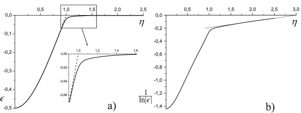
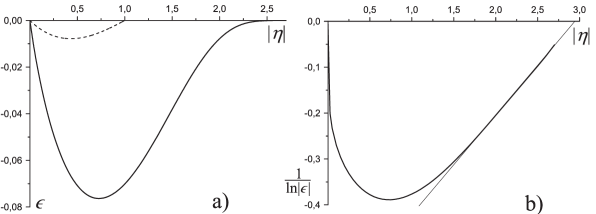
Figure 1: a) the dependency of the ground state energy on the metamass of the tachyon mediator of interaction (in the dimensionless variables $\epsilon$, $\eta$) for the ”attraction” case $\alpha<0$: solid line – numerical results, dashed line – variational approximation; b) asymptotical behavior of the energy for $1<\eta<3$.

Figure 2: The same as in Figure 1, but for the ”repulsion” case $\alpha>0$.

4 Conclusions

In the two-particle problem with the tachyon exchange interaction we limit ourselves by the non-relativistic consideration and analyze the Schrödinger equation with the anti-shielding potential, i.e., the Coulomb potential modulated by $2\pi/\mu$ periodical cosine (2).

Since the exact solution of this equation is unknown, the variational and numeral methods were applied. With the former it is proved that bound states exist at both the negative and positive coupling constant $\alpha$ for the metamass $\mu=\eta\,m|\alpha|$ in the range $0<\eta<1$. The numeral calculations indicate the existence of bound states for $1\leq\eta\leq 2.5$ too. Moreover, the ground state binding energy goes down quickly by increase of the metamass such that $|{\cal E}/{\cal E}_{\rm Ry}|<10^{-9}$ at $\eta=2.5$. Numeral integration for $\eta>2.5$ becomes overwhelming and do not provide reliable results. The extrapolation of the dependency of ${\cal E}$ on the metamass in the area $\eta>2.5$ suggests further decrease of the binding energy up to zero at $\eta_{\rm c}\simeq 3$, or $\mu_{\rm c}\simeq 3m|\alpha|$. Thus bound states exist for $\mu<\mu_{\rm c}$ or, in terms of imaginary Debye radius, for $|r_{\rm D}|>a_{\rm B}/3$. The Sedov method [34, 35] does not work in the present case, thus an exact or, at least, a precise (if finite) value of the critical parameter $\eta_{\rm c}$ is an open question.

References

- [1] O.-M. Bilaniuk, V. K. Deshpande and E. C. G. Subarshan, Amer. J. Phys. 30, 718 (1962).
- [2] O.-M. Bilaniuk, V. K. Deshpande and E. C. G. Subarshan, Physics Today 22, 43 (1969).
- [3] E. Recami and R. Mignani, Riv. Nuovo Cim. 4, 209 (1974).
- [4] E. Recami, Riv. Nuovo Cim. 9, 1 (1986).
- [5] G. Feinberg, Phys. Rev. 159, 1089 (1967).
- [6] K. Kamoi and S. Kamefuchi, Prog. Theor. Phys. 45, 1646 (1971).
- [7] E. Recami, J. Phys.: Conf. Ser. 196, 012020 (2009).
- [8] D. J. Gross and J. Perry, Phys. Rev. D 25, 330 (1982).
- [9] A. Rebhan, Nucl. Phys. B 351, 706 (1991).
- [10] D. G. Barci, C. G. Bollini and M. C. Rocca, Internat. J. Mod. Phys. A 10, 1737 (1995).
- [11] A. V. Marshakov, Physics–Uspekhi, 45, 977 (2002).
- [12] A. Sen, Internat. J. Theor. Phys. 20, 5513 (2005).
- [13] E. C. G. Sudarshan, Phys. Rev. D 1, 2428 (1970).
- [14] Ch. Jue, Phys. Rev. D 8, 1757 (1973).
- [15] E. van der Spuy, Phys. Rev. D 7, 1106 (1973).
- [16] G. D. Maccarrone and E. Recami, Nuovo Cim. A 57, 85 (1980).
- [17] A. M. Gleeson, M. G. Gundzik, E. C. G. Sudarshan and A. Pagnamenta, Phys. Rev. D 6, 807 ( 1972).
- [18] J. A. Wheeler and R. P. Feynman, Rev. Mod. Phys. 17, 157 (1945).
- [19] J. A. Wheeler and R. P. Feynman, Rev. Mod. Phys. 21, 425 (1949).
- [20] F. Hoyle and J. V. Narilikar, Action at a distance in physics and cosmology (New York, Freemen, 1974).
- [21] F. Hoyle and J. V. Narilikar, Rev. Mod. Phys. 67, 113 (1995).
- [22] R. P. Gaida and V. I. Tretyak, Acta Phys. Pol. B 11, 502 (1980).
- [23] V. I. Tretyak, Forms of relativistic Lagrangian dynamics (Kyïv, Naukova Dumka, 2011) [in Ukrainian].
- [24] M. Barham and J. W. Darewych, J. Phys. A 31, 3481 (1998).
- [25] B. Ding and J. Darewych, J. Phys. G 26, 907 (2000).
- [26] J. Darewych, Condens. Matter Phys. 3, 633 (2000).
- [27] A. Duviryak and J. W. Darewych, J. Phys. A 37, 8365 (2004).
- [28] M. Emami-Razavi and J. W. Darewych, J. Phys. G 31, 1095 (2005).
- [29] I. Zagladko and A. Duviryak, J. Phys. Studies 16, 3101 (2012).
- [30] J.-Q. Shen, Phys. Scripta 68, 87 (2003).
- [31] T. Chiueh and Y.-H. Tseng, Astrophys. J. 544, 204 (2000).
- [32] S. Flügge, Practical quantum mechanics I (Berlin-Heidelberg-NY, Springer-Verlag, 1971).
- [33] L. Landau and E. Lifshitz, Quantum Mechanics: Non-Relativistic Theory, Vol. 3 (Oxford, Pergamon Press, 1981).
- [34] V. L. Sedov. Sov. Phys. Dokl. 14, 871 (1970).
- [35] R. Dutt, Phys. Lett. A 77, 229 (1980).