Combining complex and radial slave boson fields within the Kotliar-Ruckenstein representation of correlated impurities

Abstract

The gauge symmetry group of any slave boson representation allows to gauge away the phase of bosonic fields. One benefit of this radial field formulation is the elimination of spurious Bose condensations when saddle-point approximation is performed. Within the Kotliar-Ruckenstein representation, three of the four bosonic fields can be radial while the last one has to remain complex. In this work, we present the procedure to carry out the functional integration involving constrained fermionic fields, complex bosonic fields, and radial bosonic fields. The correctness of the representation is verified by exactly evaluating the partition function and the Green’s function of the Hubbard model in the atomic limit.

1 Introduction

The challenges posed by strongly correlated electron systems have been tackled using slave-boson approaches in a number of ways. The most popular ones are probably Barnes’ [1, 2] and Kotliar and Ruckenstein’s (KR) [3] representations, as well as their multiband and rotation invariant generalizations [4, 5, 6, 7, 8]. For instance, it has been proposed that strong correlation effects taking place in the plates of a capacitor can enhance its capacitance [9].

Any slave boson representation possesses a gauge symmetry group. Regarding Barnes’ representation to the infinite-$U$ single-impurity Anderson model, it involves one doublet of fermions, one slave boson, and one time-independent constraint. Its $U(1)$ gauge symmetry may be used to gauge away the phase of the slave boson at the price of introducing a time-dependent constraint field [10, 11, 12]. While the argument was initially put forward in the continuum limit, a path integral representation on discrete time steps for the remaining radial slave boson together with the time-dependent constraint has been proposed by one of us [13]. A toy model has been analyzed, with the result that the exact expectation value of the radial slave boson is generically finite [14]. Thereby a way to exactly handle functional integrals involving constrained fermions and radial slave bosons could be put forward. Furthermore, a saddle-point approximation involving the complex slave boson field is intimately tied to a Bose condensation, that is generally viewed as spurious. On the contrary, radial slave bosons do not Bose condense, as they are deprived of a phase degree of freedom, and their saddle-point amplitude approximates their – generically finite – exact expectation value.

The KR representation [3], and related slave-boson representations [5, 6], have been set up for the Hubbard model, allowing to obtain a whole range of valuable results. In particular, they have been used to describe anti-ferromagnetic [15], spiral [16, 17, 18, 19], and striped [20, 21, 22, 23, 24] phases. Furthermore, the competition between the latter two has been addressed as well [25]. Besides, it has been obtained that the spiral order continuously evolves to the ferromagnetic order in the large $U$ regime ($U\gtrsim 60t$) [19] so that it is unlikely to be realized experimentally. Consistently, in the two-band model, ferromagnetism was found as a possible groundstate only in the doped Mott insulating regime [26]. Yet, adding a ferromagnetic exchange coupling was shown to bring the ferromagnetic instability line into the intermediate coupling regime [27]. A similar effect has been obtained with a sufficiently large next-nearest-neighbor hopping amplitude [28] or going to the fcc lattice [29].

The KR representation again implies one doublet of fermions, but now subjected to four slave bosons through three constraints. The gauge symmetry group of the representation has been debated over the years [30, 15, 31, 32], but a consensus that it reads $U(1)\times U(1)\times U(1)$ has been reached [33, 6, 34]. Hence, the phase of three of the four slave bosons can be gauged away, therefore leaving us with one single complex field. It can be the $d$-field which accounts for doubly occupied sites, or the $e$-field which accounts for empty sites. These fields are primarily associated with charge fluctuations, and one might wonder about the consequences of this asymmetry on the charge fluctuation spectrum. It turns out that the latter is independent of the choice, at least when computed to one-loop order around the paramagnetic saddle-point [35, 36].

Explicitly taking the above gauge symmetry into account yields a new type of problem from the path integral point of view: how can one simultaneously handle constrained fermionic fields, complex bosonic fields, and radial boson fields? The purpose of this work is to show that the partition function and the Green’s function of the isolated correlated impurity can be exactly calculated in this situation, in contrast to earlier works where all slave boson fields were taken as radial fields [13, 14, 37].

2 Model

We investigate an exactly soluble model, the single-site Hubbard Hamiltonian

$${\mathcal{H}}=\epsilon\sum_{\sigma}c^{\dagger}_{\sigma}c^{\phantom{\dagger}}_{\sigma}+Uc^{\dagger}_{\uparrow}c^{\phantom{\dagger}}_{\uparrow}c^{\dagger}_{\downarrow}c^{\phantom{\dagger}}_{\downarrow}.$$ (1)

The KR representation of this model implies one doublet of fermions $\{f_{\uparrow},f_{\downarrow}\}$ and four slave bosons $\{e,p_{\uparrow},p_{\downarrow},d\}$. The latter are tied to an empty site, single occupancy of the site with spin projection up or down, and double occupancy, respectively. The redundant degrees of freedom are discarded provided the three constraints

$$e^{\dagger}e+\sum_{\sigma}p^{\dagger}_{\sigma}p^{\phantom{\dagger}}_{\sigma}+d^{\dagger}d = 1$$

$$f^{\dagger}_{\sigma}f^{\phantom{\dagger}}_{\sigma}-p^{\dagger}_{\sigma}p^{\phantom{\dagger}}_{\sigma}-d^{\dagger}d = 0\;\;\;\;\;\;\;\;\;\;(\sigma=\uparrow,\downarrow)$$ (2)

are satisfied. In the functional integral formalism the latter are enforced by the Lagrange multipliers $\lambda$, resp. $\lambda_{\sigma}$. At this stage it should be noted that the functional integral over the fermionic and bosonic fields cannot be performed right away. Indeed, in order to ensure the convergence, $\lambda$ has to be continued into the complex plane as

$$\tilde{\lambda}\equiv\lambda-\mathrm{i}\lambda_{0}$$ (3)

with $\lambda_{0}>0$ (or $\lambda_{0}+U>0$ if $U<0$) so that the integration contour is shifted into the lower half-plane [38, 39, 13].

Hence the Lagrangian

$${\mathcal{L}}(\tau)={\mathcal{L}}_{f}(\tau)+{\mathcal{L}}_{b}(\tau)$$ (4)

consists of a fermionic contribution,

$${\mathcal{L}}_{f}(\tau)=\sum_{\sigma}f^{\dagger}_{\sigma}(\tau)\left(\partial_{\tau}+\epsilon+\mathrm{i}\lambda_{\sigma}\right)f^{\phantom{\dagger}}_{\sigma}(\tau),$$ (5)

and a bosonic one,

$${\mathcal{L}}_{b}(\tau) = -\mathrm{i}\lambda+e^{\dagger}(\tau)\left(\partial_{\tau}+\mathrm{i}\lambda\right)e(\tau)$$ (6)

$$+\;d^{\dagger}(\tau)\left(\partial_{\tau}+U+\mathrm{i}\lambda-\mathrm{i}\lambda_{\uparrow}-\mathrm{i}\lambda_{\downarrow}\right)d(\tau)$$

$$+\;\sum_{\sigma}p^{\dagger}_{\sigma}(\tau)\left(\partial_{\tau}+\mathrm{i}\lambda-\mathrm{i}\lambda_{\sigma}\right)p^{\phantom{\dagger}}_{\sigma}(\tau).$$

It entails the dynamics of the auxiliary fermionic and bosonic fields, together with the constraints (2) specific to the Kotliar and Ruckenstein setup.

In this representation, the physical electron creation and annihilation operators read

$$\begin{array}[]{l}c_{\sigma}^{\phantom{\dagger}}\leadsto\left(e^{\dagger}p_{\sigma}^{\phantom{\dagger}}+p_{-\sigma}^{\dagger}d\right)f_{\sigma}^{\phantom{\dagger}}\\ c_{\sigma}^{\dagger}\leadsto\left(p_{\sigma}^{\dagger}e+d^{\dagger}p_{-\sigma}^{\phantom{\dagger}}\right)f_{\sigma}^{\dagger}\end{array}$$ (7)

This representation of the physical electron operators is invariant under the gauge transformations

$$\left\{\begin{array}[]{l}f_{\sigma}\longrightarrow\mathrm{e}^{-\mathrm{i}\chi_{\sigma}}f_{\sigma}\\ e_{\phantom{\sigma}}\longrightarrow\mathrm{e}^{\mathrm{i}\theta}e\\ p_{\sigma}\longrightarrow\mathrm{e}^{\mathrm{i}\left(\chi_{\sigma}+\theta\right)}p_{\sigma}\\ d_{\phantom{\sigma}}\longrightarrow\mathrm{e}^{\mathrm{i}\left(\chi_{\uparrow}+\chi_{\downarrow}+\theta\right)}d\end{array}\right.$$ (8)

The gauge symmetry group is therefore $U(1)\times U(1)\times U(1)$. The Lagrangian, Eq. (4), also possesses this symmetry. Expressing the bosonic fields in amplitude and phase variables as

$$e(\tau) = \sqrt{R_{e}(\tau)}\,\mathrm{e}^{\mathrm{i}\theta(\tau)}$$

$$p^{\phantom{\dagger}}_{\sigma}(\tau) = \sqrt{R_{\sigma}(\tau)}\,\mathrm{e}^{\mathrm{i}(\chi_{\sigma}(\tau)+\theta(\tau))}$$ (9)

allows to gauge away the phases of three of the four slave boson fields provided one introduces the three time-dependent Lagrange multipliers

$$\alpha(\tau) \equiv \lambda+\partial_{\tau}\theta(\tau)$$

$$\beta_{\sigma}(\tau) \equiv \lambda_{\sigma}-\partial_{\tau}\chi_{\sigma}(\tau).$$ (10)

Here the radial slave boson fields are implemented in the continuum limit following, e. g., Ref. [10, 11, 12].

3 Partition function

3.1 Cartesian slave boson representation

First we evaluate the partition function with the Cartesian representation of the slave boson fields:

$${\mathcal{Z}} = \int_{-\pi/\beta}^{\pi/\beta}\frac{\beta d\!\lambda}{2\pi}\prod_{\sigma}\frac{\beta d\!\lambda_{\sigma}}{2\pi}\int\prod_{\sigma}D[f^{\phantom{\dagger}}_{\sigma},f^{\dagger}_{\sigma}]$$ (11)

$$\times\int D[e,e^{\dagger}]D[d,d^{\dagger}]\prod_{\sigma}D[p^{\phantom{\dagger}}_{\sigma},p^{\dagger}_{\sigma}]$$

$$\times\;\;\mathrm{e}^{-\int_{0}^{\beta}d\tau{\mathcal{L}}(\tau)}.$$

Note that the constraints are constants of motion since they commute with the Hamiltonian, which does not hybridize the auxiliary boson states. They may hence be enforced by time-independent constraints. Therefore one can first sum over all states, and afterward restrict the partition function to the physical subspace by imposing the constraints.

Integrating the auxiliary fermionic and bosonic fields yields

$${\mathcal{Z}} =\int_{-\pi/\beta}^{\pi/\beta}\frac{\beta d\!\lambda}{2\pi}\prod_{\sigma}\frac{\beta d\!\lambda_{\sigma}}{2\pi}$$

$$\times \frac{\mathrm{e}^{\mathrm{i}\beta\tilde{\lambda}}\prod\limits_{\sigma}\left(1+\mathrm{e}^{-\beta(\epsilon+\mathrm{i}\lambda_{\sigma})}\right)}{\left(1-\mathrm{e}^{-\mathrm{i}\beta\tilde{\lambda}}\right)\left(1-\mathrm{e}^{-\beta\left(U+\mathrm{i}\left(\tilde{\lambda}-\lambda_{\uparrow}-\lambda_{\downarrow}\right)\right)}\right)\prod\limits_{\sigma}\left(1-\mathrm{e}^{-\mathrm{i}\beta\left(\tilde{\lambda}-\lambda_{\sigma}\right)}\right)}.$$

At this point one may introduce new variables $x\equiv\mathrm{e}^{-\mathrm{i}\beta\lambda_{\uparrow}}$, $y\equiv\mathrm{e}^{-\mathrm{i}\beta\lambda_{\downarrow}}$, and $z\equiv\mathrm{e}^{-\mathrm{i}\beta\lambda}$, so that evaluating $\mathcal{Z}$ results in contour integrals along the complex unit circle $\mathbb{U}$ in the clockwise direction:

$${\mathcal{Z}} =\,\left(\frac{\mathrm{i}}{2\pi}\right)^{3}\oint_{\mathbb{U}}d\!x\,d\!y\,d\!z$$

$$\times \frac{x\,y\>\mathrm{e}^{\beta\lambda_{0}}\left(1+x\mathrm{e}^{-\beta\epsilon}\right)\left(1+y\mathrm{e}^{-\beta\epsilon}\right)}{z^{2}(1-z\mathrm{e}^{-\beta\lambda_{0}})(xy-z\mathrm{e}^{-\beta(U+\lambda_{0})})(x-z\mathrm{e}^{-\beta\lambda_{0}})(y-z\mathrm{e}^{-\beta\lambda_{0}})}.$$

One is then ready to evaluate the integral over $z$. Since $\lambda_{0}>0$ for positive $U$ ($\lambda_{0}+U>0$ otherwise), all poles are located outside $\mathbb{U}$ but the one at the origin. Hence, the $z$-contour integral only picks up the residue at $z=0$. Thus

$${\mathcal{Z}} = \left(\frac{\mathrm{i}}{2\pi}\right)^{2}\oint_{\mathbb{U}}d\!x\,d\!y\frac{1}{xy}\left(1+\frac{1}{x}+\frac{1}{y}+\frac{\mathrm{e}^{-\beta U}}{xy}\right)$$ (14)

$$\times\;\left(1+x\mathrm{e}^{-\beta\epsilon}\right)\left(1+y\mathrm{e}^{-\beta\epsilon}\right),$$

which is actually independent of the value of $\lambda_{0}$. Yet, we remind the reader that it takes a positive value of $\lambda_{0}$ to obtain Eq. (14). Finally the remaining integrations yield the expected result

$${\mathcal{Z}}=1+2\mathrm{e}^{-\beta\epsilon}+\mathrm{e}^{-\beta(2\epsilon+U)}.$$ (15)

This gives a strong indication that this representation is faithful.

3.2 Radial slave boson representation

For the exact evaluation of the functional integrals, the representation in the radial gauge has to be set on a discretized time mesh from the beginning. Moreover, the constraints now have to be satisfied at every time step. Extending the procedure introduced in Ref. [13] for Barnes’ slave boson to the Kotliar and Ruckenstein representation one can cast the partition function

$${\mathcal{Z}}=\lim_{N\rightarrow\infty}\lim_{\eta\rightarrow 0^{+}}{\mathcal{P}}{Z}_{f}{Z}_{d}$$ (16)

as a projection onto the physical subspace of the product of the auxiliary fermions partition function with the $d$ boson partition function. Here we introduced

$${\mathcal{P}}=\prod_{n=1}^{N}{\mathcal{P}}_{n}$$ (17)

with

$${\mathcal{P}}_{n} = \int_{-\infty}^{\infty}\frac{\delta d\!\alpha_{n}}{2\pi}\frac{\delta d\!\beta_{\uparrow,n}}{2\pi}\frac{\delta d\!\beta_{\downarrow,n}}{2\pi}\int_{-\eta}^{\infty}d\!R_{e,n}d\!R_{\uparrow,n}d\!R_{\downarrow,n}$$ (18)

$$\times\;\mathrm{e}^{-\mathrm{i}\delta\left((\alpha_{n}-\mathrm{i}\lambda_{0})(R_{e,n}+R_{\uparrow,n}+R_{\downarrow,n}-1)-\sum_{\sigma}\beta_{\sigma,n}R_{\sigma,n}\right)}$$

which is defined on one time step $n$ only. The variable $R_{e,n}$ ($R_{\sigma,n}$) corresponds to the amplitude of the complex $e_{n}$ ($p_{\sigma,n}$) bosonic field, and $\delta\equiv\beta/N$. Note that it takes an infinitesimal regulator $-\eta$ for the integration bounds to have well defined delta functions enforcing the constraints. As previously discussed, the functional integral has to be evaluated with $\alpha$ replaced by ($\alpha-\mathrm{i}\lambda_{0}$) where $\lambda_{0}>0$, in order to ensure convergence.

The fermionic contribution to the action is bi-linear, and is given for each spin projection by

$${\mathcal{S}}_{\sigma} =\sum_{i=1}^{N}\sum_{j=1}^{N}f^{\dagger}_{\sigma,i}[S_{\sigma}]_{i,j}f_{\sigma,j}$$

$$=\sum_{n=1}^{N}f^{\dagger}_{\sigma,n}\Big{(}f_{\sigma,n}-f_{\sigma,n-1}\mathrm{e}^{-\delta(\epsilon+\mathrm{i}\beta_{\sigma,n})}\Big{)}$$ (19)

with $f_{\sigma,0}\equiv-f_{\sigma,N}$ in the second line to satisfy anti-periodic boundary conditions. It yields the auxiliary fermion partition function

$${Z}_{f}=Z_{\uparrow}Z_{\downarrow}$$ (20)

with

$${Z}_{\sigma} =\int\!\!D[f^{\phantom{\dagger}}_{\sigma},f^{\dagger}_{\sigma}]\;\mathrm{e}^{-{\mathcal{S}}_{\sigma}}=\det[S_{\sigma}]$$

$$=1+\mathrm{e}^{-\beta\epsilon}\prod_{n=1}^{N}\mathrm{e}^{-\mathrm{i}\delta\beta_{\sigma,n}}.$$ (21)

The contribution to the action from the bosonic field $d$ is given by

$${\mathcal{S}}_{d} =\sum_{i=1}^{N}\sum_{j=1}^{N}d^{\dagger}_{i}[S_{d}]_{i,j}d_{j}$$

$$=\sum_{n=1}^{N}d^{\dagger}_{n}\Big{(}d_{n}-d_{n-1}\mathrm{e}^{-\delta(U+\mathrm{i}\tilde{\alpha}_{n}-\mathrm{i}\beta_{\uparrow,n}-\mathrm{i}\beta_{\downarrow,n})}\Big{)}$$ (22)

with $d_{\sigma,0}\equiv d_{\sigma,N}$ in the second line to satisfy periodic boundary conditions. Moreover we introduced the shorthand notation

$$\tilde{\alpha}\equiv\alpha-\mathrm{i}\lambda_{0}.$$ (23)

One therefore obtains

$${Z}_{d} = \int\!\!D[d,d^{\dagger}]\;\mathrm{e}^{-{\mathcal{S}}_{d}}=\det[S_{d}]^{-1}$$ (24)

$$= \left(1-\mathrm{e}^{-\beta U}\prod_{n=1}^{N}\mathrm{e}^{-\mathrm{i}\delta(\tilde{\alpha}_{n}-\beta_{\uparrow,n}-\beta_{\downarrow,n})}\right)^{-1}.$$

When expanding the exponential in Eqs. (3.2,3.2) to lowest order in $\delta$, the familiar form following from the Trotter-Suzuki decomposition is recovered. Yet, the latter may only be applied for a finite value of $\beta_{\sigma,n}$ while Eqs. (3.2,3.2) are well behaved even for $\beta_{\sigma,n}\rightarrow\infty$, as shown below.

Let us now address the projection of ${Z}_{f}{Z}_{d}$ onto the physical subspace. Two alternative procedures may be considered: i) First integrate over the radial slave boson fields and then perform the integration over the constraint fields, or ii) First perform the integration over the constraint fields, and then compute the integration over the radial slave bosons. We address them in this order.

3.2.1 Integrating the radial bosons first

Integrating the radial boson amplitudes yields

$${\mathcal{P}}_{n}=\int_{-\infty}^{\infty}\frac{d\!\alpha_{n}}{2\mathrm{i}\pi}\frac{\mathrm{e}^{\mathrm{i}\delta(1+\eta)\tilde{\alpha}_{n}}}{\tilde{\alpha}_{n}}\prod_{\sigma}\frac{d\!\gamma_{\sigma,n}}{2\mathrm{i}\pi}\frac{\mathrm{e}^{-\mathrm{i}\delta\eta\tilde{\gamma}_{\sigma,n}}}{\tilde{\gamma}_{\sigma,n}}$$ (25)

with

$$\gamma_{\sigma,n}\equiv\beta_{\sigma,n}-\alpha_{n}\>,\quad\quad\tilde{\gamma}_{\sigma,n}\equiv\gamma_{\sigma,n}+\mathrm{i}\lambda_{0}.$$ (26)

The Jacobian of the transformation is unity. Then, by expanding the product ${Z}_{f}$, the discrete-time partition function is

$${\mathcal{P}}{Z}_{f}{Z}_{d} = \int_{-\infty}^{\infty}\prod_{n=1}^{N}\left(\frac{d\!\alpha_{n}}{2\mathrm{i}\pi\tilde{\alpha}_{n}}\prod_{\sigma}\frac{d\!\gamma_{\sigma,n}}{2\mathrm{i}\pi\tilde{\gamma}_{\sigma,n}}\right)$$ (27)

$$\times\;\Bigg{(}\prod_{m=1}^{N}\mathrm{e}^{\mathrm{i}\delta(1+\eta)\tilde{\alpha}_{m}}\mathrm{e}^{-\mathrm{i}\delta\eta\tilde{\gamma}_{\uparrow,m}}\mathrm{e}^{-\mathrm{i}\delta\eta\tilde{\gamma}_{\downarrow,m}}$$

$$\;\;+\;\mathrm{e}^{-\beta\epsilon}\sum_{\sigma}\prod_{m=1}^{N}\mathrm{e}^{\mathrm{i}\delta\eta\tilde{\alpha}_{m}}\mathrm{e}^{-\mathrm{i}\delta(1+\eta)\tilde{\gamma}_{\sigma,m}}\mathrm{e}^{-\mathrm{i}\delta\eta\tilde{\gamma}_{-\sigma,m}}$$

$$\;\;+\;\mathrm{e}^{-2\beta\epsilon}\prod_{m=1}^{N}\mathrm{e}^{\mathrm{i}\delta(-1+\eta)\tilde{\alpha}_{m}}\mathrm{e}^{-\mathrm{i}\delta(1+\eta)\tilde{\gamma}_{\uparrow,m}}\mathrm{e}^{-\mathrm{i}\delta(1+\eta)\tilde{\gamma}_{\downarrow,m}}\!\Bigg{)}$$

$$\times\;\left(1-\mathrm{e}^{-\beta U}\prod_{m=1}^{N}\mathrm{e}^{\mathrm{i}\delta(\tilde{\alpha}_{m}+\tilde{\gamma}_{\uparrow,m}+\tilde{\gamma}_{\downarrow,m})}\right)^{-1}.$$

In the limit $U=\infty$ where ${Z}_{d}=1$, evaluating the multiple integral is straightforward since it is only composed of products of simple integrals. The computation, however, is more intricate in the general case. It involves integrals of the form

$$I_{\xi}(r) \equiv \int_{-\infty}^{\infty}\frac{d\!x}{2\mathrm{i}\pi(x-\mathrm{i}\lambda_{0})}\>\frac{\mathrm{e}^{\mathrm{i}\delta(x-\mathrm{i}\lambda_{0})r}}{1-\xi\mathrm{e}^{\mathrm{i}\delta(x-\mathrm{i}\lambda_{0})}}\,,$$

$$J_{\xi}(r) \equiv \int_{-\infty}^{\infty}\frac{d\!x}{2\mathrm{i}\pi(x+\mathrm{i}\lambda_{0})}\>\frac{\mathrm{e}^{\mathrm{i}\delta(x+\mathrm{i}\lambda_{0})r}}{1-\xi\mathrm{e}^{\mathrm{i}\delta(x+\mathrm{i}\lambda_{0})}}\,,$$ (28)

where $r$ is a real number ($r\not\in-\mathbb{N}$), and $\xi$ is a complex exponential of other integration variables ($|\xi|<1$). Using the equalities

$$I_{\xi}(r)=I_{0}(r)+\xi I_{\xi}(r+1) \,, \quad I_{0}(r)=\hat{\theta}(r)\,,$$

$$J_{\xi}(r)=J_{0}(r)+\xi J_{\xi}(r+1) \,, \quad J_{0}(r)=-\hat{\theta}(-r)\,,$$ (29)

where $\hat{\theta}$ is the Heaviside step function, one finds that

$$I_{\xi}(r)=\sum_{k=0}^{\infty}\xi^{k}\hat{\theta}(r+k)\;\;{\rm and}\;\;J_{\xi}(r)=-\sum_{k=0}^{\infty}\xi^{k}\hat{\theta}(-r-k).$$ (30)

In particular, with $\eta\rightarrow 0^{+}$,

$$I_{\xi}({-1+\eta})=\frac{1}{1-\xi}-1\,,\quad I_{\xi}({\eta})=I_{\xi}({1+\eta})=\frac{1}{1-\xi}\,,$$ (31)

$$J_{\xi}(-1-\eta)=-1-\xi\,,\quad J_{\xi}(-\eta)=-1.$$

Integrating the variables at time step $N$ is enough to separate the resulting multiple integral into products of simple integrals. For instance with the term multiplied by $\mathrm{e}^{-2\beta\epsilon}$ in Eq. (27), which corresponds to the contribution from the doubly occupied state, the computation proceeds as follows:

$$\int_{-\infty}^{\infty}\prod_{\sigma}\left(\frac{d\!\gamma_{\sigma,N}}{2\mathrm{i}\pi\tilde{\gamma}_{\sigma,N}}\mathrm{e}^{-\mathrm{i}\delta(1+\eta)\tilde{\gamma}_{\sigma,N}}\right)\frac{d\!\alpha_{N}}{2\mathrm{i}\pi\tilde{\alpha}_{N}}\mathrm{e}^{\mathrm{i}\delta(-1+\eta)\tilde{\alpha}_{N}}{Z}_{d}$$

$$= \int_{-\infty}^{\infty}\prod_{\sigma}\left(\frac{d\!\gamma_{\sigma,N}}{2\mathrm{i}\pi\tilde{\gamma}_{\sigma,N}}\mathrm{e}^{-\mathrm{i}\delta(1+\eta)\tilde{\gamma}_{\sigma,N}}\right)I_{\xi\mathrm{e}^{\mathrm{i}\delta(\tilde{\gamma}_{\uparrow,N}+\tilde{\gamma}_{\downarrow,N})}}(-1+\eta)$$

where $\xi=\mathrm{e}^{-\beta U}\prod_{m=1}^{N-1}\mathrm{e}^{\mathrm{i}\delta(\tilde{\alpha}_{m}+\tilde{\gamma}_{\uparrow,m}+\tilde{\gamma}_{\downarrow,m})}$

$$= \int_{-\infty}^{\infty}\prod_{\sigma}\left(\frac{d\!\gamma_{\sigma,N}}{2\mathrm{i}\pi\tilde{\gamma}_{\sigma,N}}\mathrm{e}^{-\mathrm{i}\delta(1+\eta)\tilde{\gamma}_{\sigma,N}}\right)\left(\frac{1}{1-\xi\mathrm{e}^{\mathrm{i}\delta(\tilde{\gamma}_{\uparrow,N}+\tilde{\gamma}_{\downarrow,N})}}-1\right)$$ (32)

$$= \int_{-\infty}^{\infty}\frac{d\!\gamma_{\downarrow,N}}{2\mathrm{i}\pi\tilde{\gamma}_{\downarrow,N}}\mathrm{e}^{-\mathrm{i}\delta(1+\eta)\tilde{\gamma}_{\downarrow,N}}\Big{(}J_{\xi\mathrm{e}^{\mathrm{i}\delta\tilde{\gamma}_{\downarrow,N}}}(-1-\eta)-J_{0}(-1-\eta)\Big{)}$$

$$= -\xi\int_{-\infty}^{\infty}\frac{d\!\gamma_{\downarrow,N}}{2\mathrm{i}\pi\tilde{\gamma}_{\downarrow,N}}\mathrm{e}^{-\mathrm{i}\delta\eta\tilde{\gamma}_{\downarrow,N}}=-\xi J_{0}(-\eta)=\xi.$$

Hence

$${\mathcal{P}}{Z}_{d}{Z}_{f} = \int_{-\infty}^{\infty}\prod_{n=1}^{N-1}\left(\frac{d\!\alpha_{n}}{2\mathrm{i}\pi\tilde{\alpha}_{n}}\prod_{\sigma}\frac{d\!\gamma_{\sigma,n}}{2\mathrm{i}\pi\tilde{\gamma}_{\sigma,n}}\right)$$

$$\times\;\Bigg{(}\prod_{m=1}^{N-1}\mathrm{e}^{\mathrm{i}\delta(1+\eta)\tilde{\alpha}_{m}}\mathrm{e}^{-\mathrm{i}\delta\eta\tilde{\gamma}_{\uparrow,m}}\mathrm{e}^{-\mathrm{i}\delta\eta\tilde{\gamma}_{\downarrow,m}}$$

$$\quad+\;\mathrm{e}^{-\beta\epsilon}\sum_{\sigma}\prod_{m=1}^{N-1}\mathrm{e}^{\mathrm{i}\delta\eta\tilde{\alpha}_{m}}\mathrm{e}^{-\mathrm{i}\delta(1+\eta)\tilde{\gamma}_{\sigma,m}}\mathrm{e}^{-\mathrm{i}\delta\eta\tilde{\gamma}_{-\sigma,m}}$$

$$\quad+\;\mathrm{e}^{-2\beta\epsilon}\mathrm{e}^{-\beta U}\prod_{m=1}^{N-1}\mathrm{e}^{\mathrm{i}\delta\eta\tilde{\alpha}_{m}}\mathrm{e}^{-\mathrm{i}\delta\eta\tilde{\gamma}_{\uparrow,m}}\mathrm{e}^{-\mathrm{i}\delta\eta\tilde{\gamma}_{\downarrow,m}}\Bigg{)}.$$

Then integrating over the remaining $(N-1)$ time steps is straightforward, and

$${\mathcal{P}}{Z}_{d}{Z}_{f} = \left(I_{0}({1+\eta})J_{0}({-\eta})^{2}\right)^{N-1}$$ (34)

$$+\;2\mathrm{e}^{-\beta\epsilon}\left(I_{0}({\eta})J_{0}({-1-\eta})J_{0}({-\eta})\right)^{N-1}$$

$$+\;\mathrm{e}^{-\beta(2\epsilon+U)}\left(I_{0}({\eta})J_{0}({-\eta})^{2}\right)^{N-1}$$

$$= 1+2\mathrm{e}^{-\beta\epsilon}+\mathrm{e}^{-\beta(2\epsilon+U)}.$$

Even though this procedure might be seen as lacking transparency, the proper result is obtained. Let us now consider an alternative route along which one first performs the integrals over the Lagrange multipliers.

3.2.2 Integrating the Lagrange multipliers first

Integrating first the Lagrange multipliers involves evaluating integrals of the form

$$\int_{-\infty}^{\infty}\frac{\delta d\!x}{2\pi}\>\frac{\mathrm{e}^{\mathrm{i}\delta(x-\mathrm{i}\lambda_{0})r}}{1-\xi\mathrm{e}^{\mathrm{i}\delta(x-\mathrm{i}\lambda_{0})}}=\frac{\partial I_{\xi}(r)}{\partial r}=\sum_{k=0}^{\infty}\xi^{k}\hat{\delta}(r+k)$$ (35)

where $\hat{\delta}$ is the Dirac delta function. As shown below, the relation allows to write the partition function as an explicit sum over the different values of the double occupancy $|d|^{2}$. Hence, expanding ${Z}_{d}$ as a power series of $\mathrm{e}^{-\beta U}$ yields

$${\mathcal{P}}{Z}_{f}{Z}_{d}$$

$$\;={\mathcal{P}}\prod_{\sigma}\!\left(\!1+\mathrm{e}^{-\beta\epsilon}\mathrm{e}^{-\mathrm{i}\delta\!\sum\limits_{m}\beta_{\sigma,m}}\right)\!\!\sum_{k=0}^{\infty}\!\left(\!\mathrm{e}^{-\beta U}\mathrm{e}^{\mathrm{i}\delta\!\sum\limits_{m}(-\tilde{\alpha}_{m}+\beta_{\uparrow,m}+\beta_{\downarrow,m})}\right)^{\!\!k}$$

$$\;=\prod_{p=1}^{N}\bigg{(}\int_{-\eta}^{\infty}\!d\!R_{e,p}d\!R_{\uparrow,p}d\!R_{\downarrow,p}\int_{-\infty}^{\infty}\frac{\delta d\!\alpha_{p}}{2\pi}\frac{\delta d\!\beta_{\uparrow,p}}{2\pi}\frac{\delta d\!\beta_{\downarrow,p}}{2\pi}\bigg{)}$$

$$\quad\;\times\;\Bigg{\{}\sum_{k=0}^{\infty}\mathrm{e}^{-k\beta U}\prod_{n=1}^{N}\mathrm{e}^{\mathrm{i}\delta(1-k-R_{e,n}-R_{\uparrow,n}-R_{\downarrow,n})\tilde{\alpha}_{n}}$$

$$\quad\quad\times\;\bigg{(}\prod_{m=1}^{N}\mathrm{e}^{\mathrm{i}\delta(R_{\uparrow,m}+k)\beta_{\uparrow,m}}\mathrm{e}^{\mathrm{i}\delta(R_{\downarrow,m}+k)\beta_{\downarrow,m}}$$

$$\quad\quad\quad+\;\mathrm{e}^{-\beta\epsilon}\sum_{\sigma}\prod_{m=1}^{N}\mathrm{e}^{\mathrm{i}\delta(R_{\sigma,m}+k)\beta_{\sigma,m}}\mathrm{e}^{\mathrm{i}\delta(R_{-\sigma,m}+k-1)\beta_{-\sigma,m}}$$

$$\quad\quad\quad+\;\mathrm{e}^{-2\beta\epsilon}\prod_{m=1}^{N}\mathrm{e}^{\mathrm{i}\delta(R_{\uparrow,m}+k-1)\beta_{\uparrow,m}}\mathrm{e}^{\mathrm{i}\delta(R_{\downarrow,m}+k-1)\beta_{\downarrow,m}}\!\bigg{)}\Bigg{\}}.$$ (36)

Here one recognizes the Fourier transform of delta functions. So integrating the Lagrange multipliers results in

$${\mathcal{P}}{Z}_{f}{Z}_{d} = \prod_{p=1}^{N}\bigg{(}\int_{-\eta}^{\infty}d\!R_{e,p}d\!R_{\uparrow,p}d\!R_{\downarrow,p}\bigg{)}$$

$$\times\Bigg{\{}\!\sum_{k=0}^{\infty}\mathrm{e}^{-k\beta U}\prod_{n=1}^{N}\hat{\delta}\left(1-k-R_{e,n}\!-R_{\uparrow,n}\!-R_{\downarrow,n}\right)$$

$$\;\;\times\bigg{(}\prod_{m=1}^{N}\hat{\delta}(R_{\uparrow,m}\!+k)\hat{\delta}(R_{\downarrow,m}\!+k)$$

$$\quad+\;\mathrm{e}^{-\beta\epsilon}\sum_{\sigma}\prod_{m=1}^{N}\hat{\delta}(R_{\sigma,m}\!+k)\hat{\delta}(R_{-\sigma,m}\!+k-1)$$

$$\quad+\;\mathrm{e}^{-2\beta\epsilon}\prod_{m=1}^{N}\hat{\delta}(R_{\uparrow,m}\!+k-1)\hat{\delta}(R_{\downarrow,m}\!+k-1)\!\bigg{)}\!\Bigg{\}}.$$

As stated above, the partition function is obtained as a sum running over the integer values $k$ of the boson amplitude $|d|^{2}$. Then integrating the delta function $\hat{\delta}(R_{\sigma,m}+k)$ yields a non vanishing contribution only for $k=0$ because $R_{\sigma,m}\geq-\eta$. With $\hat{\delta}(R_{\sigma,m}+k-1)$, only $k=0$ and $k=1$ are retained. Thus the sum stops at $k=1$, and

$${\mathcal{P}}{Z}_{f}{Z}_{d} = \prod_{p=1}^{N}\bigg{(}\int_{-\eta}^{\infty}\!\!d\!R_{e,p}\bigg{)}\Bigg{\{}\!\bigg{(}\!\prod_{n=1}^{N}\hat{\delta}\left(1-R_{e,n}\right)$$ (38)

$$+\;2\mathrm{e}^{-\beta\epsilon}\prod_{n=1}^{N}\hat{\delta}\left(-R_{e,n}\right)+\mathrm{e}^{-2\beta\epsilon}\prod_{n=1}^{N}\hat{\delta}\left(-1-R_{e,n}\right)\!\!\bigg{)}$$

$$+\;\mathrm{e}^{-\beta U}\bigg{(}0+\mathrm{e}^{-\beta\epsilon}\times 0+\mathrm{e}^{-2\beta\epsilon}\prod_{n=1}^{N}\hat{\delta}\left(-R_{e,n}\right)\!\bigg{)}\!\Bigg{\}}$$

$$= 1+2\mathrm{e}^{-\beta\epsilon}+\mathrm{e}^{-\beta(2\epsilon+U)}.$$

The second procedure is eventually more intuitive than the first one, as the projection results in an explicit sum over the contribution of every physical state at every time step. That is why we will use it to discuss the evaluation of the Green’s function.

4 Green’s function

For the imaginary-time variable $0<\tau<\beta$, the time-ordered Green’s function is calculated as the limit of the discrete-time correlation:

$${\mathcal{Z}}{\mathcal{G}}_{\uparrow}(\tau,0)=-\langle c_{\uparrow}^{\phantom{\dagger}}(\tau)c_{\uparrow}^{\dagger}(0)\rangle=-\lim_{N\rightarrow\infty}\langle c_{\uparrow,m}^{\phantom{\dagger}}c_{\uparrow,1}^{\dagger}\rangle$$ (39)

with $\lim\limits_{N\rightarrow\infty}\left(\frac{m\beta}{N}\right)=\tau$. Using the KR representation, Eq. (7), one obtains the correlation $\langle c_{\uparrow,m}^{\phantom{\dagger}}c_{\uparrow,1}^{\dagger}\rangle$ as the sum of the formal projections $P$ onto the physical subspace of the correlations of two kinds of processes within the augmented Fock space of auxiliary boson states:

$$P\left[\big{(}e^{\dagger}p_{\uparrow}^{\phantom{\dagger}}f_{\uparrow}\big{)}_{m}\big{(}p_{\uparrow}^{\dagger}ef_{\uparrow}^{\dagger}\big{)}_{1}\right]+P\left[\big{(}p_{\downarrow}^{\dagger}df_{\uparrow}^{\phantom{\dagger}}\big{)}_{m}\big{(}d^{\dagger}p_{\downarrow}^{\phantom{\dagger}}f_{\uparrow}^{\dagger}\big{)}_{1}\right].$$ (40)

The first process involves variations of $e$ and $p_{\uparrow}$ boson numbers. When restricted to the physical subspace, it generates the transitions $|0\rangle\rightarrow|\!\uparrow\rangle\rightarrow|0\rangle$ between the physical states, while the second process, with variations of $d$ and $p_{\downarrow}$ boson numbers, corresponds to the transitions $|\!\downarrow\rangle\rightarrow|\!\uparrow\downarrow\rangle\rightarrow|\!\downarrow\rangle$.

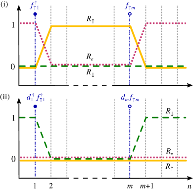
Figure 1: (Color online) Time evolution of constrained radial fields during the transitions (i) $|0\rangle\rightarrow|\!\uparrow\rangle\rightarrow|0\rangle$, and (ii) $|\!\downarrow\rangle\rightarrow|\!\uparrow\downarrow\rangle\rightarrow|\!\downarrow\rangle$, generated by the creation of an electron with spin up at time step 1, and its annihilation at time step $m>1$. The values of $R_{\uparrow}$, $R_{\downarrow}$, and $R_{e}$ are plotted respectively with solid, dashed, and dotted lines.

Calculating functional integrals with the Cartesian representation of complex bosonic fields is standard [40]. For instance, at time $\tau_{n}=\frac{n\beta}{N}$, the operators $e$ and $e^{\dagger}$ yield, respectively, the complex fields $e_{n-1}$ and $e_{n}^{\dagger}$ in the discrete-time action. So the number operator $e^{\dagger}e$ results in the value $e_{n}^{\dagger}e_{n-1}$. For the radial representation, an original procedure has to be devised [13]. It has been found that the latter contribution to the action can be computed with the real field $R_{e,n}$, which describes the boson amplitude $|e|^{2}$. However, in the correlation Eq. (40) the annihilation and creation operators act at different times. The issue is then how to integrate terms involving a single operator $e$ or $e^{\dagger}$. One could imagine having the license to use either $\sqrt{R_{e,n-1}}$ or $\sqrt{R_{e,n}}$. However, this is not the case. As shown in details below, when the dynamics of the $d$-boson and $f$-fermion fields are imposed, the physical constraints (2) strictly select the radial-field trajectories that contribute to the functional integral. These constrained evolutions are plotted in Fig. 1 for the two processes generated by the creation of an electron at time step 1, followed by its annihilation at time step $m$. Hence, in order to obtain non-vanishing correlations and the correct result for the Green’s function, the proper choice of time steps for the radial fields is necessarily

$$\big{(}e^{\dagger}p_{\uparrow}^{\phantom{\dagger}}f_{\uparrow}\big{)}_{m}\big{(}p_{\uparrow}^{\dagger}ef_{\uparrow}^{\dagger}\big{)}_{1} \leadsto\sqrt{R_{e,m+1}R_{\uparrow,m}}f_{\uparrow,m}\sqrt{R_{\uparrow,2}^{\phantom{\dagger}}R_{e,1}}f_{\uparrow,1}^{\dagger}$$

$$\big{(}p_{\downarrow}^{\dagger}df_{\uparrow}^{\phantom{\dagger}}\big{)}_{m}\big{(}d^{\dagger}p_{\downarrow}^{\phantom{\dagger}}f_{\uparrow}^{\dagger}\big{)}_{1} \leadsto\sqrt{R_{\downarrow,m+1}}d_{m}f_{\uparrow,m}d_{1}^{\dagger}\sqrt{R_{\downarrow,1}}f_{\uparrow,1}^{\dagger}.$$ (41)

This is obtained with the representations for the electron annihilation and creation fields

$$\begin{array}[]{l}c_{\uparrow,n}\leadsto\left(\sqrt{R_{e,n+1}R_{\uparrow,n}}+\sqrt{R_{\downarrow,n+1}}d_{n}\right)f_{\uparrow,n}^{\phantom{\dagger}}\\ c_{\uparrow,n}^{\dagger}\leadsto\left(\sqrt{R_{\uparrow,n+1}R_{e,n}}+d_{n}^{\dagger}\sqrt{R_{\downarrow,n}}\right)f_{\uparrow,n}^{\dagger}\end{array}$$ (42)

which are the generalization for finite on-site repulsion of the forms obtained in [13] for the Barnes representation, and in [37] for the KR representation in the limit of infinite $U$. Eq. (42) also serves to express the hybridization term of the single-impurity Anderson Model within this auxiliary particles framework.

Specifically, the projected correlation for the first process may be computed using Eqs. (17,18) as

$$P\Big{[}\big{(}e^{\dagger}p_{\uparrow}^{\phantom{\dagger}}f_{\uparrow}\big{)}_{m}\big{(}p_{\uparrow}^{\dagger}ef_{\uparrow}^{\dagger}\big{)}_{1}\Big{]}$$

$$=\lim_{\eta\rightarrow 0^{+}}{\mathcal{P}}\left\langle\sqrt{R_{e,m+1}R_{\uparrow,m}}f_{\uparrow,m}\sqrt{R_{\uparrow,2}^{\phantom{\dagger}}R_{e,1}}f_{\uparrow,1}^{\dagger}\right\rangle$$

$$=\lim_{\eta\rightarrow 0^{+}}{\mathcal{P}}\left(\sqrt{R_{e,m+1}R_{\uparrow,m}R_{\uparrow,2}R_{e,1}}Z_{d}\left\langle f_{\uparrow,m}^{\phantom{\dagger}}f_{\uparrow,1}^{\dagger}\right\rangle Z_{\downarrow}\right).$$ (43)

The angle brackets in the second line stand for the integration over the trajectories of the $f_{\sigma}$ and $d$ fields, which yields the partition functions given by Eqs. (3.2,24), and

$$\left\langle f_{\uparrow,m}^{\phantom{\dagger}}f_{\uparrow,1}^{\dagger}\right\rangle =\int\!\!\!D[f^{\phantom{\dagger}}_{\uparrow},f^{\dagger}_{\uparrow}]\;f_{\uparrow,m}^{\phantom{\dagger}}f_{\uparrow,1}^{\dagger}\;\mathrm{e}^{-{\mathcal{S}}_{\uparrow}}$$

$$=[S_{\uparrow}^{-1}]_{m,1}\det[S_{\uparrow}]=\prod_{n=2}^{m}\mathrm{e}^{-\delta(\epsilon+\mathrm{i}\beta_{\uparrow,n})}.$$ (44)

As in the previous section, expanding $Z_{d}$ in power series of $\mathrm{e}^{-\beta U}$ results in a sum over the integer values $k$ of $|d|^{2}$. The latter actually stops at $k=0$. Indeed, integrating out the Lagrange multipliers Fourier transforms the complex exponentials into delta functions, and it turns out that every term in the sum contains a product $\prod\limits_{n=2}^{m}\hat{\delta}(R_{\uparrow,n}+k)$. Since $R_{\uparrow,n}\geq 0$, only $k=0$ actually produces a non vanishing contribution. Thus the projected correlation can be written as

$$P\Big{[}\big{(}e^{\dagger}p_{\uparrow}^{\phantom{\dagger}}f_{\uparrow}\big{)}_{m}\big{(}p_{\uparrow}^{\dagger}ef_{\uparrow}^{\dagger}\big{)}_{1}\Big{]}=\mathrm{e}^{-\delta(m-1)\epsilon}\prod_{n=1}^{N}\left(\int_{0^{-}}^{+\infty}\!\!\!\!\!dR_{e,n}\,\prod_{\sigma}dR_{\sigma,n}\right)$$

$$\times\sqrt{R_{e,m+1}R_{\uparrow,m}R_{\uparrow,2}R_{e,1}}\;\prod_{n_{1}=1}^{N}\hat{\delta}\big{(}R_{e,n_{1}}+R_{\uparrow,n_{1}}+R_{\downarrow,n_{1}}-1\big{)}$$

$$\times\left(\prod_{n_{2}=1}^{N}\hat{\delta}(R_{\downarrow,n_{2}})+\mathrm{e}^{-\beta\epsilon}\prod_{n_{2}=1}^{N}\hat{\delta}(R_{\downarrow,n_{2}}-1)\right)$$

$$\times\prod_{i_{1}\in\llbracket 2,m\rrbracket}\hat{\delta}(R_{\uparrow,i_{1}}-1)\prod_{i_{2}\notin\llbracket 2,m\rrbracket}\hat{\delta}(R_{\uparrow,i_{2}})$$ (45)

(in the product, ${i_{2}\notin\llbracket 2,m\rrbracket}$ is a shorthand notation for the integer values $i_{2}=1$ or $m+1\leq i_{2}\leq N$). The expression shows that only one trajectory of the radial fields contribute to the functional integral. This is the constrained evolution depicted in Fig. 1, in which $R_{\uparrow,n}=1$ for $2\leq n\leq m$ and $R_{\uparrow,n}=0$ otherwise, $R_{e,n}=1-R_{\uparrow,n}$ and $R_{\downarrow,n}=0$. And, as a result,

$$P\Big{[}\big{(}e^{\dagger}p_{\uparrow}^{\phantom{\dagger}}f_{\uparrow}\big{)}_{m}\big{(}p_{\uparrow}^{\dagger}ef_{\uparrow}^{\dagger}\big{)}_{1}\Big{]}=\mathrm{e}^{-\delta(m-1)\epsilon}.$$ (46)

For the second process,

$$P\Big{[}\big{(}p_{\downarrow}^{\dagger}df_{\uparrow}^{\phantom{\dagger}}\big{)}_{m}\big{(}d^{\dagger}p_{\downarrow}^{\phantom{\dagger}}f_{\uparrow}^{\dagger}\big{)}_{1}\Big{]}$$

$$=\lim_{\eta\rightarrow 0^{+}}{\mathcal{P}}\left\langle\sqrt{R_{\downarrow,m+1}}d_{m}f_{\uparrow,m}d_{1}^{\dagger}\sqrt{R_{\downarrow,1}}f_{\uparrow,1}^{\dagger}\right\rangle$$

$$=\lim_{\eta\rightarrow 0^{+}}{\mathcal{P}}\left(\sqrt{R_{\downarrow,m+1}R_{\downarrow,1}}\left\langle d_{m}^{\phantom{\dagger}}d_{1}^{\dagger}\right\rangle\left\langle f_{\uparrow,m}^{\phantom{\dagger}}f_{\uparrow,1}^{\dagger}\right\rangle Z_{\downarrow}\right)$$ (47)

where $\left\langle d_{m}^{\phantom{\dagger}}d_{1}^{\dagger}\right\rangle$ is obtained as

$$\left\langle d_{m}^{\phantom{\dagger}}d_{1}^{\dagger}\right\rangle =\int\!\!\!D[d,d^{\dagger}]\;\;d_{m}^{\phantom{\dagger}}d_{1}^{\dagger}\;\mathrm{e}^{-{\mathcal{S}}_{d}}$$

$$=\frac{[S_{d}^{-1}]_{m,1}}{\det[S_{d}]}=Z_{d}^{2}\prod\limits_{n=2}^{m}\mathrm{e}^{-\delta\big{(}U+\mathrm{i}(\tilde{\alpha}_{n}-\beta_{\uparrow,n}-\beta_{\downarrow,n})\big{)}}.$$ (48)

Expanding now $Z_{d}^{2}$ and integrating out the Lagrange multipliers result in

$$P\Big{[}\big{(}p_{\downarrow}^{\dagger}df_{\uparrow}^{\phantom{\dagger}}\big{)}_{m}\big{(}d^{\dagger}p_{\downarrow}^{\phantom{\dagger}}f_{\uparrow}^{\dagger}\big{)}_{1}\Big{]}$$

$$=\mathrm{e}^{-\delta(m-1)(U+\epsilon)}\prod_{n=1}^{N}\left(\int_{0^{-}}^{+\infty}\!\!\!\!\!dR_{e,n}\,\prod_{\sigma}dR_{\sigma,n}\right)\sqrt{R_{\uparrow,m+1}R_{\downarrow,1}}$$

$$\times\prod_{i_{1}=2}^{m}\!\hat{\delta}\big{(}R_{e,i_{1}}+R_{\uparrow,i_{1}}+R_{\downarrow,i_{1}}\big{)}\prod_{i_{2}\notin\llbracket 2,m\rrbracket}\!\!\!\!\!\hat{\delta}\big{(}R_{e,i_{2}}+R_{\uparrow,i_{2}}+R_{\downarrow,i_{2}}-1\big{)}$$

$$\times\prod_{n_{1}=1}^{N}\hat{\delta}(R_{\uparrow,n_{1}})\times\left(\prod_{j_{1}=2}^{m}\hat{\delta}(R_{\downarrow,j_{1}}+1)\prod_{j_{2}\notin\llbracket 2,m\rrbracket}\hat{\delta}(R_{\downarrow,j_{2}})\right.$$

$$\quad\left.+\mathrm{e}^{-\beta\epsilon}\prod_{l_{1}=2}^{m}\hat{\delta}(R_{\downarrow,l_{1}})\prod_{l_{2}\notin\llbracket 2,m\rrbracket}\hat{\delta}(R_{\downarrow,l_{2}}-1)\right).$$ (49)

Among all the trajectories, only the second one shown in Fig. 1 yields a non-vanishing contribution: the delta functions impose that $R_{\downarrow,n}=0$ for $2\leq n\leq m$ and $R_{\downarrow,n}=1$ otherwise, while $R_{\uparrow,n}=R_{e,n}=0$ for each time step. Hence after integrating over the radial variables, the second projected correlation is

$$P\Big{[}\big{(}p_{\downarrow}^{\dagger}df_{\uparrow}^{\phantom{\dagger}}\big{)}_{m}\big{(}d^{\dagger}p_{\downarrow}^{\phantom{\dagger}}f_{\uparrow}^{\dagger}\big{)}_{1}\Big{]}=\mathrm{e}^{-\delta(m-1)(U+\epsilon)}\mathrm{e}^{-\beta\epsilon}.$$ (50)

Lastly, in the limit $N\rightarrow\infty$, the expected expression for the Green’s function is obtained as

$${\mathcal{Z}}{\mathcal{G}}_{\uparrow}(\tau,0)=-\left(\mathrm{e}^{-\tau\epsilon}+\mathrm{e}^{-\tau(U+\epsilon)}\mathrm{e}^{-\beta\epsilon}\right).$$ (51)

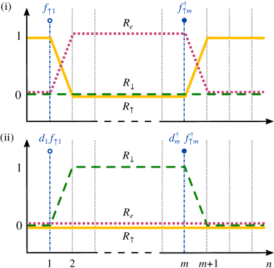
Figure 2: (Color online) Time evolution of constrained radial fields during the transitions (i) $|\!\uparrow\rangle\rightarrow|0\rangle\rightarrow|\!\uparrow\rangle$, and (ii) $|\!\uparrow\downarrow\rangle\rightarrow|\!\downarrow\rangle\rightarrow|\!\uparrow\downarrow\rangle$, generated by the annihilation of an electron with spin up at time step 1, and its creation at time step $m>1$. The values of $R_{\uparrow}$, $R_{\downarrow}$, and $R_{e}$ are plotted respectively with solid, dashed, and dotted lines.

The same procedure can be applied to calculate the time-ordered Green’s function

$${\mathcal{Z}}{\mathcal{G}}_{\uparrow}(0,\tau)=\langle c_{\uparrow}^{\dagger}(\tau)c_{\uparrow}^{\phantom{\dagger}}(0)\rangle=\lim_{N\rightarrow\infty}\langle c_{\uparrow,m}^{\dagger}c_{\uparrow,1}^{\phantom{\dagger}}\rangle.$$ (52)

Here the annihilation of an electron with spin up at time step 1, followed by the creation of another one at $m>1$, produces two possible series of transitions between the physical states: $|\!\uparrow\rangle\rightarrow|0\rangle\rightarrow|\!\uparrow\rangle$, and $|\!\uparrow\downarrow\rangle\rightarrow|\!\downarrow\rangle\rightarrow|\!\uparrow\downarrow\rangle$. The correlation $\langle c_{\uparrow,m}^{\dagger}c_{\uparrow,1}^{\phantom{\dagger}}\rangle$ is then the sum of the projected correlations

$$P\Big{[}\big{(}p_{\uparrow}^{\dagger}ef_{\uparrow}^{\dagger}\big{)}_{m}\big{(}e^{\dagger}p_{\uparrow}^{\phantom{\dagger}}f_{\uparrow}^{\phantom{\dagger}}\big{)}_{1}\Big{]}$$

$$=\lim_{\eta\rightarrow 0^{+}}{\mathcal{P}}\left\langle\sqrt{R_{\uparrow,m+1}^{\phantom{\dagger}}R_{e,m}^{\phantom{\dagger}}}f_{\uparrow,m}^{\dagger}\sqrt{R_{e,2}^{\phantom{\dagger}}R_{\uparrow,1}^{\phantom{\dagger}}}f_{\uparrow,1}^{\phantom{\dagger}}\right\rangle$$ (53)

and

$$P\Big{[}\big{(}d^{\dagger}p_{\downarrow}^{\phantom{\dagger}}f_{\uparrow}^{\dagger}\big{)}_{m}\big{(}p_{\downarrow}^{\dagger}d^{\phantom{\dagger}}f_{\uparrow}^{\phantom{\dagger}}\big{)}_{1}\Big{]}$$

$$=\lim_{\eta\rightarrow 0^{+}}{\mathcal{P}}\left\langle\sqrt{R_{\downarrow,m}^{\phantom{\dagger}}}d_{m}^{\phantom{\dagger}}f_{\uparrow,m}^{\dagger}\sqrt{R_{\downarrow,2}^{\phantom{\dagger}}}d_{1}^{\phantom{\dagger}}f_{\uparrow,1}^{\phantom{\dagger}}\right\rangle,$$ (54)

with

$$\left\langle f_{\uparrow,m}^{\dagger}f_{\uparrow,1}^{\phantom{\dagger}}\right\rangle=\prod_{n\notin\llbracket 2,m\rrbracket}\mathrm{e}^{-\delta(\epsilon+\mathrm{i}\beta_{\uparrow,n})}$$ (55)

and

$$\left\langle d_{m}^{\dagger}d_{1}^{\phantom{\dagger}}\right\rangle=Z_{d}^{2}\prod_{n\notin\llbracket 2,m\rrbracket}\mathrm{e}^{-\delta\big{(}U+\mathrm{i}(\tilde{\alpha}_{n}-\beta_{\uparrow,n}-\beta_{\downarrow,n})\big{)}}.$$ (56)

This radial representation of the correlations is obtained from the discrete-time prescriptions (42) as well. It is the only choice of time-steps that yields non-vanishing integrals, as illustrated by Fig. 2 which displays the constrained evolutions of the radial fields for the physical transitions involved here. Then projecting the sum onto the physical subspace, that is integrating out the Lagrange multipliers and the radial boson fields, results in the expected correlation for the Green’s function

$${\mathcal{Z}}{\mathcal{G}}_{\uparrow}(0,\tau) =\lim_{N\rightarrow\infty}\left(\mathrm{e}^{-\delta(N-m+1)\epsilon}+\mathrm{e}^{-\beta\epsilon}\mathrm{e}^{-\delta(N-m+1)(\epsilon+U)}\right)$$

$$=\mathrm{e}^{-(\beta-\tau)\epsilon}+\mathrm{e}^{-\beta\epsilon}\mathrm{e}^{-(\beta-\tau)(\epsilon+U)}.$$ (57)

Higher order Green’s functions may be calculated by means of the same procedure.

5 Summary and conclusion

In this work, we have considered the Kotliar and Ruckenstein slave boson representation of the Hubbard Model in the radial gauge. It allows to gauge away the phase of three of the four involved slave boson fields. As a result, the functional integral representation of the partition function, of the Green’s function and of correlation functions involves canonical fermionic and bosonic fields, together with radial slave boson fields. The correctness of this functional integral representation has been verified through the exact calculation of the partition function and the Green’s function in the atomic limit. Furthermore, the proper representation of the physical electron creation and annihilation operators, that is crucial to the representation of the kinetic energy operator, has been established. This paves the way for calculations of larger systems and can also be applied to the single-impurity Anderson model.

References

- [1] S. E. Barnes, J. Phys. F 1976, 6, 1375.
- [2] S. E. Barnes, J. Phys. F 1977, 7, 2637.
- [3] G. Kotliar and A. E. Ruckenstein, Phys. Rev. Lett. 1986, 57, 1362.
- [4] R. Frésard and G. Kotliar, Phys. Rev. B 1997, 56, 12909.
- [5] T. C. Li, P. Wölfle, and P. J. Hirschfeld, Phys. Rev. B 1989, 40, 6817.
- [6] R. Frésard and P. Wölfle, Int. J. of Mod. Phys. B 1992, 6, 685; 1992, 6, 3087.
- [7] F. Lechermann, A. Georges, G. Kotliar, and O. Parcollet, Phys. Rev. B 2007, 76, 155102.
- [8] C. Piefke and F. Lechermann, Phys. Rev. B 2018, 97, 125154.
- [9] K. Steffen, R. Frésard, and T. Kopp, Phys. Rev. B 2017, 95, 035143.
- [10] N. Read, D. M. Newns, J. Phys. C 1983, 16, L1055.
- [11] N. Read, D. M. Newns, J. Phys. C 1983, 16, 3273.
- [12] D. M. Newns and N. Read, Adv. in Physics 1987, 36, 799.
- [13] R. Frésard and T. Kopp, Nucl. Phys. B 2001, 594, 769.
- [14] R. Frésard, H. Ouerdane, and T. Kopp, Nucl. Phys. B 2007, 785, 286.
- [15] L. Lilly, A. Muramatsu, and W. Hanke, Phys. Rev. Lett. 1990, 65, 1379.
- [16] R. Frésard, M. Dzierzawa, and P. Wölfle, Europhys. Lett. 1991, 15, 325.
- [17] P. A. Igoshev, M. A. Timirgazin, A. K. Arzhnikov, and V. Y. Irkhin, JETP Lett. 2013, 98, 150.
- [18] R. Frésard and P. Wölfle, J. Phys.: Condens. Matter 1992, 4, 3625.
- [19] B. Möller, K. Doll, and R. Frésard, J. Phys.: Condens. Matter 1993, 5, 4847.
- [20] G. Seibold, E. Sigmund, and V. Hizhnyakov, Phys. Rev. B 1998, 57, 6937.
- [21] M. Fleck, A. I. Lichtenstein, and A. M. Oleś, Phys. Rev. B 2001, 64, 134528.
- [22] J. Lorenzana and G. Seibold, Phys. Rev. Lett. 2002, 89, 136401; 2003, 90, 066404; 2005, 94, 107006.
- [23] M. Raczkowski, R. Frésard, and A. M. Oleś, Phys. Rev. B 2006, 73, 174525.
- [24] M. Raczkowski, M. Capello, D. Poilblanc, R. Frésard, and A. M. Oleś, Phys. Rev. B 2007, 76, 140505(R).
- [25] M. Raczkowski, R. Frésard, and A. M. Oleś, Europhys. Lett. 2006, 76, 128.
- [26] R. Frésard and M. Lamboley, J. Low Temp. Phys. 2002, 126, 1091.
- [27] G. Lhoutellier, R. Frésard, and A. M. Oleś, Phys. Rev. B 2015, 91, 224410.
- [28] R. Frésard and W. Zimmermann, Phys. Rev. B 1998, 58, 15288.
- [29] P.A. Igoshev, M.A. Timirgazin, V.F. Gilmutdinov, A.K. Arzhnikov, V.Yu. Irkhin, J. Phys: Condens. Matter 2015, 27, 446002.
- [30] J. W. Rasul and T. Li, J. Phys. C: Solid State Phys. 1988, 21, 5119.
- [31] M. Lavagna, Phys. Rev. B 1990, 41, 142.
- [32] T. Li and P. Bénard, Phys. Rev. B 1994, 50, 17837.
- [33] Th. Jolicœur and J. C. Le Guillou, Phys. Rev. B 1991, 44, 2403.
- [34] Y. Bang, C. Castellani, M. Grilli, G. Kotliar, R. Raimondi, and Z. Wang, Int. J. of Mod. Phys. B 1992, 6, 531; Proceedings of the Adriatico Research Conference and Miniworkshop Strongly Correlated Electrons Systems III, eds. Yu Lu, G. Baskaran, A. E. Ruckenstein, E. Tossati (World Scientific Publishing Co., Singapore, 1992).
- [35] V. H. Dao and R. Frésard, Phys. Rev. B 2017, 95, 165127.
- [36] V. H. Dao and R. Frésard, Acta Phys. Pol. A 2018, 133, 336.
- [37] R. Frésard and T. Kopp, Ann. Phys. (Berlin) 2012, 524, 175.
- [38] N. E. Bickers, Ph.D. Thesis, Cornell University, 1986.
- [39] N. E. Bickers, Rev. Mod. Phys. 1987, 59, 845.
- [40] J. W. Negele and H. Orland, Quantum Many-Particle Systems (Westview Press, Boulder, Colorado, 1998).